European Spallation Source as a searching tool for an ultralight scalar field

Abstract

Dark matter (DM) nature is one of the major issues in physics. The search for a DM candidate has motivated the known proposal of an ultralight scalar field (ULSF). We explore the possibility to search for this ULSF at the upcoming European Spallation Source neutrino Super-Beam experiment. We have considered the recent study case in which there could be an interaction between the ULSF and active neutrinos. We have found that in this future experimental setup, the sensitivity is competitive with other neutrino physics experiments. We show the expected future sensitivity for the main parameter modeling the interaction between ULSF and neutrinos.

I Introduction

The existence of dark matter (DM) is one of the most intriguing aspects of modern cosmology. Nearly one fourth of the matter-energy content of the Universe is in the form of dark matter and elucidating its nature is a very fundamental issue. There are plenty of proposals to model dark matter, from objects like primordial black holes with masses of the order of $2\times 10^{21}$ Kg ($10^{57}$ eV/$c^{2}$), weakly interacting massive particles (WIMPs) with masses around $100$ TeV/$c^{2}-$2 GeV/$c^{2}$, axions with masses of $10^{-5}$ eV/$c^{2}$, or ultralight scalar dark matter particles with masses of $10^{-22}$ eV/$c^{2}$.

One of the proposals for a dark matter candidate postulates that an ultralight relativistic scalar field $\phi$ can model dark matter with a suitable scalar potential $V(\phi)$ Sahni and Wang (2000); Hu et al. (2000); Matos et al. (2000); Matos and Urena-Lopez (2000); Arbey et al. (2002, 2001) (see, for example, the following reviews Magana and Matos (2012); Suárez et al. (2014); Marsh (2016); Hui et al. (2017); Lee (2018); Ureña López (2019)). The general property of this scalar field potential is the existence of a parabolic minimum around which it is possible to define a mass scale for the related boson particle. In this model, the galactic halos can be formed by condensing the scalar field at the Universe’s beginning Magana and Matos (2012). The successful physical implications of $\Lambda$CDM at cosmological scales are replicated by the scalar field dark matter, e.g., the evolution of the cosmological densities Matos et al. (2009), the acoustic peaks of the cosmic microwave background radiation (CMBR) Rodriguez-Montoya et al. (2010), the rotations curves in big- and low-surface brightness (LSB) galaxies Lesgourgues et al. (2002); Arbey et al. (2003); Harko (2011); Robles and Matos (2012), and the observed properties of dwarf galaxies Lee and Lim (2010).

Besides, the oscillations of the scalar field could have exciting and important physical consequences. Since neutrinos have small masses, the interaction with the oscillations of the scalar field could have a relevant influence on neutrino masses and mixing. Considering that the mechanism of neutrino masses is still unknown, the interaction with the oscillating scalar field could provide a link to physics beyond the Standard Model (SM). The former reasons constitute a strong motivation to study the effects of a light scalar field in neutrino oscillations.

More recently, searches for an ultralight scalar field at neutrino oscillation experiments are becoming possible (see, e.g., Refs. Berlin (2016); Brdar et al. (2018); Krnjaic et al. (2018); Liao et al. (2018); Kim et al. (2020); Dev et al. (2021); Losada et al. (2022a)) due to advancements in the energy resolution of present and upcoming neutrino oscillation experiments. Besides, feasible cosmological models of active and/or sterile neutrinos interacting with an ultralight scalar field have been explored Zhao (2017); Farzan (2019); Cline (2020); Dev et al. (2022); Huang et al. (2022). In Ref. Losada et al. (2022b), the implications for the reactor neutrino experiments Kamioka liquid-scintillator antineutrino detector (KamLAND) and Jiangmen Underground Neutrino Observatory (JUNO) due to interactions between active neutrinos and a scalar field with mass $m_{\phi}\gtrsim 10^{-12}$ eV/$c^{2}$ are considered. Despite these interesting studies, it is important to notice that such an interaction between neutrinos and the ultralight scalar field (ULSF) may also lead to tension with current experimental observables, as we will discuss below. Moreover, recent studies corner the ultralight dark matter (ULDM) proposal to be only a subdominant component of the DM content Kobayashi et al. (2017); Bar:2021kti . Still, the interaction of a neutrino with a ULSF can be of interest independently of its connection to the DM problem.

In this paper, we will explore the phenomenological consequences of having an ultralight scalar field mixed with the neutrino mass eigenstates and the capabilities of an European Spallation Source Neutrino Super Beam (ESS$\nu$SB)-like experiment Baussan et al. (2014); Alekou et al. (2021, 2022) to constraint these interactions. The original proposal is to study a neutrino Super Beam, which employs the European Spallation Source (ESS) facility as a neutrino source with a water Cherenkov detector Agostino et al. (2013) located in a deep mine, for the discovery of the Dirac $CP$-violating phase $\delta$. We consider two baselines. One at 360 km, corresponding to the distance from the source to the Zinkgruvan mine. While the second would be at 540 km, with a detector placed at the Garpenberg mine; both mines are located in Sweden. Moreover, scenarios that investigate the capabilities of the ESS$\nu$SB experiment to probe physics beyond the Standard Model and neutrino oscillations have been discussed Kumar Agarwalla et al. (2019); Ghosh et al. (2020); Choubey et al. (2021); Majhi et al. (2021); Blennow et al. (2020a); Chatterjee et al. (2021); Ahn et al. (2022).

The structure of the paper is as follows. In Sec. II, we present one possible form of interaction between neutrinos and the ultralight scalar field. This interaction modifies the leptonic mixing angle $\theta$, and adds a smearing on the neutrino mass squared difference $\Delta m^{2}$. Section III explains the characteristics and assumptions made in the general long baseline experiment simulator (GLoBES) software Huber et al. (2005, 2007) to simulate the ESS$\nu$SB experiment. Sensitivities to the ULSF via modulations from average distorted neutrino oscillations are developed in Sec. IV. Finally, we give our conclusions.

II Framework

The existence of dark matter has stimulated extensive and intensive activity to explain its characteristics. There are a plethora of possible candidates for dark matter. In this section, we will mention some of the more studied proposals. For example, primordial black holes could have been formed soon after the big bang from the gravitational collapse of higher-density mass regions. Some constraints restrict the masses of primordial black holes to several windows between $10^{13}-10^{14}$ kg, $10^{17}-10^{21}$ kg, and $10-10^{3}$ solar masses ($2\times 10^{30}$ kg) Carr and Kuhnel (2020). However, from latest results of LIGO and VIRGO, it seems that primordial black holes only provide some part of the needed amount of dark matter Carr et al. (2021).

The main characteristics that must fulfill a possible particle candidate for dark matter are that it has to be stable over billions of years, nonrelativistic, massive, and weakly interacting. The Standard Model of particle physics does not have a particle with these properties.

One of the most studied extensions of the Standard Model is its minimal supersymmetric extension (MSSM) Arbey and Mahmoudi (2021); several candidates for WIMPs can emerge in this model. The possible candidates for dark matter are neutralinos, gravitinos, and sneutrinos. The neutralino is the most studied particle candidate for dark matter; it has been extensible searched at the LHC. In the LEP and Tevatron experiments, a lower-mass bound around 46 GeV/$c^{2}$ has been set Arbey and Mahmoudi (2021). The gravitino couples very weakly to other particles; therefore, it is challenging to impose any constraint on it Arbey and Mahmoudi (2021). The lightest sneutrino is strongly interacting, which is unsuitable for a dark matter particle.

Another popular dark matter candidate is the axion, a light neutral particle that can be produced in the early Universe by a spontaneous symmetry breaking of $U_{a}(1)$ Peccei-Quin symmetry Arbey and Mahmoudi (2021); Di Luzio et al. (2020). Experimental attempts have been developed to detect the axions using the prediction that axions and photons could be transformed into each other in an intense magnetic field Arun et al. (2017).

Besides the former candidates for dark matter, there are other massive particles like sterile neutrinos that only interact gravitationally, with masses around $\mathcal{O}$(keV/$c^{2}$) Drewes (2013); Ng et al. (2019).

Furthermore, other exotic dark matter candidates exist like WIMPzillas, strongly interacting massive particles (SIMPs), Q-nuggets, Q-balls, gluinos, Fermi balls, EW balls, GUT balls, etc. The masses of these objects range from 100 GeV/$c^{2}$ to a TeV/$c^{2}$ Arun et al. (2017); Oks (2021).

Another approach consists of avoiding the existence of massive dark matter particles or objects and instead considering modifications of gravitational interactions, for example, modified newtonian dynamics (MOND) Milgrom (1983); Baker et al. (2021) and extra dimensions Randall and Sundrum (1999a, b).

Regarding the scalar-field dark matter, there are some problems that this proposal can solve. For example, on the cosmological side there are problems with certain predictions of $\Lambda$CDM at the galactic scale. Some examples are the excess of substructures produced in $N$-body numerical simulations, which are one order of magnitude larger than the observed ones, and the cusp profile of central density in galactic halos Clowe et al. (2006); Klypin et al. (1999); Moore et al. (1999). Additionally, problems arise in numerical simulations of structure formation, which do not produce pure disk galaxies, among other problems. The former problems could be avoided if the structure grew faster than in $\Lambda$CDM Peebles and Nusser (2010).

Some of the former problems are resolved in the ultralight relativistic scalar field framework. In this model, the galactic halos are formed by a Bose-Einstein condensation of a scalar boson with a mass around $m_{\phi}\sim 10^{-22}$ eV/$c^{2}$.

The Compton length associated with this boson is of the order of kpc, which is the same order as the size of dark halos in typical galaxies. It is proposed that the dark halos are very big drops of scalar field. Then, when the Universe reaches the critical temperature of condensation, all galactic halos form at the same time producing well-formed halo galaxies at high $z$, which is a different prediction from $\Lambda$CDM Lee and Lim (2010).

The scalar field dark matter can resolve the problem of cusp profile of density in galactic halos since this is avoided due to the wave properties of the ultralight mass of the scalar particles Hu et al. (2000); Lundgren et al. (2010). Furthermore, the excess of substructures is prevented by considering that the scalar field has a natural cutoff Hu et al. (2000); Matos and Urena-Lopez (2001); Suarez and Matos (2011).

Although we consider here a scalar boson mass, $m_{\phi}\sim 10^{-22}$ eV/$c^{2}$, it is important to mention that this value can change from different physical constraints and different astrophysical models. Except for some few models Arvanitaki et al. (2010); Cicoli et al. (2022), all the justification for this mass region comes from consistency with astrophysical observations. For example, from the anisotropies of the CMB, the mass of the scalar field could be in the range of $m_{\phi}=10^{-24}-10^{-22}$ eV/$c^{2}$ Ureña López (2019). From galaxy rotation curves, the ULDM mass lies in the region $m_{\phi}=0.5\times 10^{-23}-10^{-21}$ eV/$c^{2}$ Bernal et al. (2018); Ureña López et al. (2017).

In addition, it is expected that the ULDM cannot be the total fraction of the dark matter if the mass is light enough, although the exact value might be model dependent. For instance, the combined analysis of CBM and large-scale structure (LSS) data sets Hlozek et al. (2015) allow ULDM masses $m_{\phi}\gtrsim 10^{-24}$ eV/$c^{2}$ if $\rho_{\phi}\sim\rho_{\text{DM}}$ and as low as $m_{\phi}\sim 10^{-27}$ eV/$c^{2}$ if $\rho_{\phi}\sim 0.05\rho_{\text{DM}}$. Lyman-$\alpha$ forest excludes ULDM masses lighter than $m_{\phi}\lesssim 10^{-21}$ eV/$c^{2}$ if $\rho_{\phi}\sim\rho_{\text{DM}}$ while a ULDM mass $m_{\phi}\sim 10^{-22}$ eV/$c^{2}$ can be accommodated if $\rho_{\phi}\lesssim 0.2\rho_{\text{DM}}$ Kobayashi et al. (2017). On the other hand, from the soliton-halo relation, a ULDM with mass below $m_{\phi}\sim 10^{-21}$ eV/$c^{2}$ is disfavored Bar:2018acw . Moreover, Ref. Bar:2021kti suggests that the ULSF is not the total component of cosmological DM, if the mass range is $10^{-24}\leavevmode\nobreak\ \lesssim m_{\phi}\leavevmode\nobreak\ (\text{eV}/c^{2})\leavevmode\nobreak\ \lesssim 10^{-20}$, while admitting it for $\rho_{\phi}\lesssim 0.3\rho_{\text{DM}}$. Finally, constraints from structure formation Arvanitaki et al. (2015) exclude ULDM masses lighter than $m_{\phi}\sim 10^{-20}$ eV/$c^{2}$ if $\rho_{\phi}\sim\rho_{\text{DM}}$ while the bound disappears when $\rho_{\phi}\lesssim 0.1\rho_{\text{DM}}$.

Let us review some of the main characteristics of the scalar field framework, which are relevant to our work. From the Lagrangian density for the scalar field

$$\mathcal{L}=\frac{1}{2}\nabla_{\mu}\phi\nabla^{\mu}\phi+V(\phi),$$ (1)

the conservation of the energy-momentum tensor $\nabla_{\mu}T^{\mu\nu}=0$ in the cosmological background of the Friedmann-Lemaitre-Robertson-Walker metric gives

$$\ddot{\phi}+3H\dot{\phi}+V^{\prime}(\phi)=0,$$ (2)

where $H=\dot{a}/a$ is the Hubble parameter and $a$ is the scale factor of the Universe. In the following, we will use natural units where $c=\hbar=1$. The scalar energy density is Magana and Matos (2012)

$$T_{0}^{0}=\frac{1}{2}\dot{\phi}^{2}+V(\phi)=\rho_{\phi}.$$

The evolution of the scalar field can be obtained numerically near the minimum of the potential where $V^{\prime}(\phi)=m^{2}_{\phi}\phi$. The contribution from the other components of matter-energy density present in the Universe is included in the Friedmann equation

$$H^{2}=\frac{8\pi G}{3}(\rho_{r}+\rho_{m}+\rho_{\phi}+\rho_{\Lambda}),$$ (3)

and $\rho_{r}$, $\rho_{m}$, and $\rho_{\Lambda}$ are the energy densities associated with radiation, baryonic nonrelativistic matter, and dark energy, respectively. However, there are analytical approximations for the scalar fields in recent times when $H_{0}\sim 10^{-33}$ eV and $H_{0}\ll m_{\phi}$. It has been proposed Magana and Matos (2012) the following anzats for the scalar field

$$\phi=2\sqrt{\hat{\rho}}\cos(S-m_{\phi}t)\,\,.$$ (4)

In late times, the scalar field behaves as nonrelativistic, and the relation $\dot{S}/m_{\phi}\sim 0$ is fulfilled when the temperature at which the scalar field begins to oscillate is $T_{\text{osc}}\sim$ keV corresponding to a redshift $z_{\text{osc}}\sim 10^{6}$ Hui et al. (2017) if $m_{\phi}\sim 10^{-22}$ eV.

From the evolution equation for the scalar field Eq. (2), $\hat{\rho}=\hat{\rho}_{0}a^{-3}$ is obtained, which is proportional to the energy density of non-relativistic matter. From the expression of the scalar-field energy density, it is possible to obtain $\rho_{\phi}=2m^{2}_{\phi}\hat{\rho}$. The ultralight scalar field can be described by a classical field minimally coupled to gravity Urena-Lopez (2007). For instance, by setting the phase $S=\pi/2$ and writing the scalar field in terms of the energy density, we can have a ULSF that oscillates with time as

$$\phi\simeq\phi_{0}\sin(m_{\phi}t),$$ (5)

with $m_{\phi}\sim 10^{-22}$ eV and

$$\phi_{0}\simeq\frac{\sqrt{2\rho_{\phi}}}{m_{\phi}},$$ (6)

where $\rho_{\phi}$ is the field density at the surface of the Earth, which we will assume to be $0.3$ GeV/cm³, $\rho_{\phi}\leq\rho_{\text{DM},\odot}=0.3$ GeV/cm³. From recent analyses, the estimation of the local DM density coincide within a range of $\rho_{\text{DM},\odot}\simeq 0.3-0.6\leavevmode\nobreak\ \text{GeV/cm}^{3}$ de Salas et al. (2019); de Salas and Widmark (2021); Sivertsson et al. (2022).

If we consider that this scalar field can interact with the neutrino, a modification in the leptonic mixing angle $\theta$ or additional smearing on the neutrino mass-squared difference $\Delta m^{2}$ will arise. Recently, the possible interaction between the ULSF and neutrinos and its implications have been considered Berlin (2016); Farzan (2019); Dev et al. (2021); Losada et al. (2022a). In this case, the ULSF can produce an effect on neutrino oscillations. Besides the SM Lagrangian, we would have an additional contribution due to the hypothetical ULSF interaction with the neutrino Berlin (2016); Losada et al. (2022a)

$$\mathcal{L}_{\lambda,y}\supset\frac{\lambda^{\alpha\beta}}{\Lambda}(L_{\alpha})^{\text{T}}L_{\beta}HH+\frac{y^{\alpha\beta}}{\Lambda^{2}}\phi(L_{\alpha})^{\text{T}}L_{\beta}HH,$$ (7)

where $\lambda^{\alpha\beta}$ and $y^{\alpha\beta}$ are 3$\times$3 dimensionless symmetric matrices, and $\Lambda$ is the scale of new physics.

$$\mathcal{L}_{m_{\nu}}\supset\frac{\lambda^{\alpha\beta}v^{2}}{2\Lambda}(\nu_{\alpha})^{\text{T}}\nu_{\beta}+\frac{y^{\alpha\beta}v^{2}}{2\Lambda^{2}}\phi(\nu_{\alpha})^{\text{T}}\nu_{\beta}.$$ (8)

After symmetry breaking and replacement of the Higgs field $H$ by its vacuum expectation value $\braket{H}=1/\sqrt{2}\leavevmode\nobreak\ (0,v)^{T}$, the neutrino mass matrix acquires corrections from the ULSF field $\phi$:

$$\tilde{m}=m_{\nu}+\hat{y}\phi;\leavevmode\nobreak\ \leavevmode\nobreak\ m_{\nu}=\frac{\lambda v^{2}}{\Lambda}\leavevmode\nobreak\ \leavevmode\nobreak\ \text{and}\leavevmode\nobreak\ \leavevmode\nobreak\ \hat{y}=\frac{yv^{2}}{\Lambda^{2}}.$$ (9)

For instance, the interaction term in Eqs. (7) and (8) can arise within the framework of a type I seesaw Krnjaic et al. (2018).

If we consider the off-diagonal $\hat{y}$ matrix elements, we will obtain a correction to the leptonic mixing angle. In a $2\times 2$ neutrino picture, the mixing matrix for this case will have the form

$$\tilde{m}=m_{\nu}+\hat{y}\phi=\left(\begin{array}[]{cc}m_{1}&\hat{y}_{12}\phi\\ \hat{y}_{12}\phi&m_{2}\\ \end{array}\right).$$ (10)

To diagonalize this matrix, we can apply a rotation, $R(\psi)$, such that $\tan(2\psi)=-2\hat{y}_{12}\phi/\Delta m$. For small angles, $\psi$, $\tan(2\psi)\approx 2\psi$ and $\psi\approx-\hat{y}_{12}\phi/\Delta m$. Once the mass matrix is diagonal, we can rotate to the flavor basis through a new transformation $R(\theta)$. Since $R(\theta)R(\psi)=R(\theta+\psi)$, then, the mixing angle receives contributions from the $\hat{y}_{12}$ term, such that $\tilde{\theta}\rightarrow\theta+\hat{y}_{12}\phi/\Delta m,\leavevmode\nobreak\ \tilde{\theta}\rightarrow\theta+\eta_{\theta}\sin m_{\phi}t$. However, our sensitivity, in this case, will be limited. Therefore, we will concentrate on the case of diagonal couplings.

In the case of two neutrino mixing, if we consider only diagonal couplings ($\alpha=\beta$), the modified $\hat{y}$ matrix up to leading order is

$$\tilde{m}^{2}=(m_{\nu}+\hat{y}\phi)^{2}\simeq\left(\begin{array}[]{cc}m_{1}^{2}+2m_{1}\hat{y}_{11}\phi&0\\ 0&m_{2}^{2}+2m_{2}\hat{y}_{22}\phi\\ \end{array}\right)+\mathcal{O}(\hat{y}^{2}\phi^{2}).$$ (11)

Therefore, for the mass squared difference, we will have

$$\Delta\tilde{{m}}^{2}_{21}\simeq m_{2}^{2}-m_{1}^{2}+2(m_{2}\hat{y}_{22}-m_{1}\hat{y}_{11})\phi.$$ (12)

or

$$\Delta\tilde{m}^{2}_{21}=\Delta m_{21}^{2}\Big{[}1+\frac{2(m_{2}\hat{y}_{22}-m_{1}\hat{y}_{11})\phi}{\Delta m_{21}^{2}}\Big{]}+\mathcal{O}(\hat{y}^{2}\phi^{2})=\Delta m_{21}^{2}\Big{[}1+2\eta_{\Delta}\sin(m_{\phi}t)\Big{]}+\mathcal{O}(\hat{y}^{2}\phi^{2}).$$ (13)

Furthermore, the ULSF parameter $\eta_{\Delta}$ is given by

$$\eta_{\Delta}=\frac{(m_{j}\hat{y}_{j}-m_{i}\hat{y}_{i})\sqrt{2\rho_{\phi}}}{\Delta m_{ji}^{2}m_{\phi}}\leavevmode\nobreak\ \leavevmode\nobreak\ \leavevmode\nobreak\ (i<j).$$ (14)

Then, we can have a modification to the neutrino conversion probability due to the shift in the neutrino mass diagonal terms,

$$P_{\mu e}\simeq\sin^{2}2\theta\sin^{2}\Big{[}\frac{\Delta m^{2}L}{4E_{\nu}}\big{(}1+2\eta_{\Delta}\sin(m_{\phi}t)\big{)}\Big{]}.$$ (15)

In the next section, we will implement the simulation of the effects of scalar field diagonal couplings in neutrino oscillations.

III Simulation

The ESS linac is projected to be fully operational at 5 MW average power with an expected 2.5 GeV proton beam currently under construction in Lund, Sweden. It will be an essential user facility providing slow neutrons for research laboratories and the industry. More importantly, for this study is the ESS$\nu$SB initiative. A neutrino super-beam facility that will benefit from the ESS production of neutrons to search for the leptonic Dirac $CP$-violating phase $\delta$ Baussan et al. (2014); Alekou et al. (2021, 2022); the data taking it is planned to start by 2035. It will investigate neutrino oscillations around the second oscillation maximum with two baselines in consideration at either 360 km or 540 km from the source. In addition to measuring the leptonic Dirac $CP$-violating phase, the ESS$\nu$SB facility may be employed to detect cosmological neutrinos and neutrinos from supernova events and measure the proton lifetime.

This section presents the characteristics and assumptions performed in our study. We use GLoBES Huber et al. (2005, 2007) to simulate an ESS$\nu$SB-like experiment with a 538 kt water Cherenkov detector Agostino et al. (2013). The information on the neutrino fluxes is taken from Fig. 3 of the original proposal Baussan et al. (2014), which corresponds to a 2.0 GeV proton beam with $2.7\times 10^{23}$ protons on target per year  fixed at 5MW. Furthermore, the neutrino fluxes have been properly rescaled to the corresponding baseline at $L=360$ km, or $L=540$ km distance, as well as renormalized to the more recent simulation with 2.5 GeV proton kinetic energy Alekou et al. (2021). The cross sections and efficiencies in the detector follow the specifications from Ref. Campagne et al. (2007). We assume an energy resolution which follows a Gaussian distribution, with a width of $\sigma(E)=12\%/\sqrt{E[\mbox{GeV}]}$ for electrons and $\sigma(E)=10\%/\sqrt{E[\mbox{GeV}]}$ for muons, respectively. A total of 12 bins uniformly distributed in the energy interval of 0.1-1.3 GeV were considered. Moreover, a 10-year exposure on a far detector is considered in the form of $5$ years in neutrino mode and $5$ years in antineutrino mode. Nevertheless, in our calibration of the expected number of signal and background events, we have assumed a one-year exposure to match the results from the updated analysis released by the ESS$\nu$SB collaboration Alekou et al. (2021). Unless otherwise specified, the systematic errors are implemented as 10$\%$ signal normalization error and 15$\%$ background normalization error for both appearance and disappearance channels. In Refs. Baussan et al. (2014); Alekou et al. (2021), the systematic errors have been considered to be $5\%$ ($10\%$) for signal (background), respectively. Ours are more conservative. Furthermore, a $0.01\%$ energy calibration error has been adopted for both types of events. Our event rates reasonably reproduce  the events reported in Tables 2 and 3 of Ref. Alekou et al. (2021).

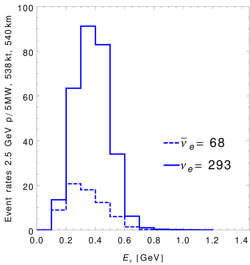
(a)

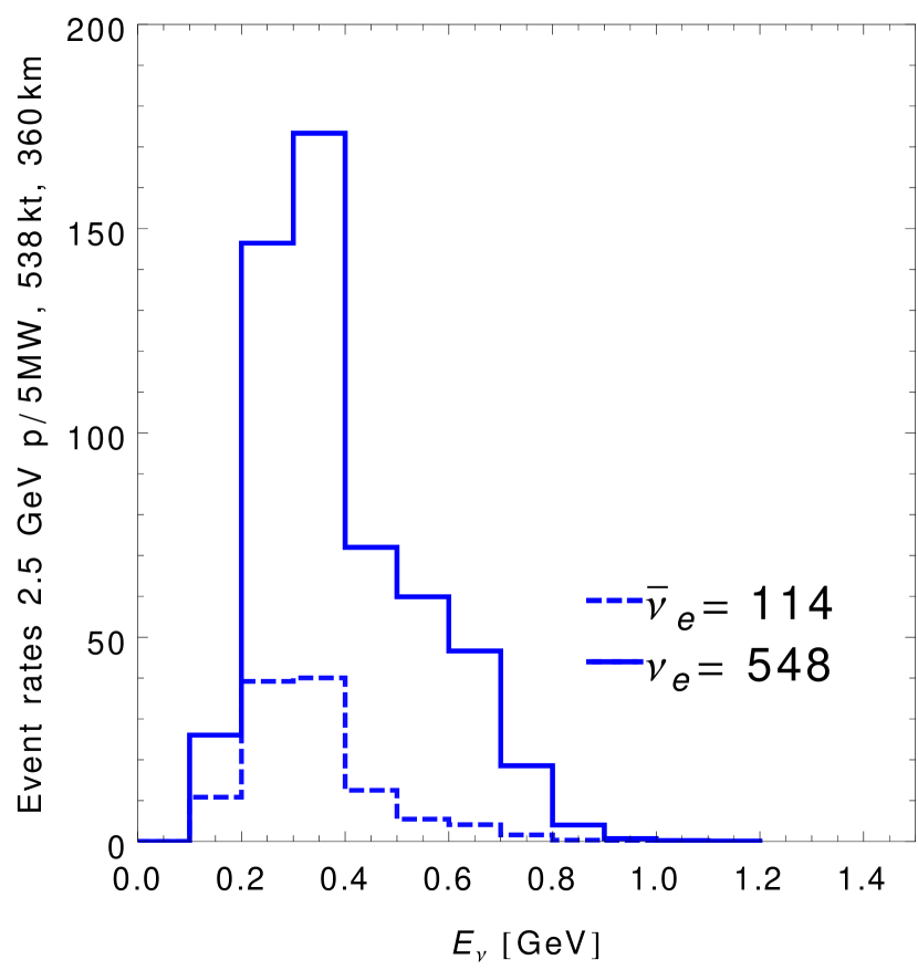
(b)

Figure 1: Expected electron-neutrino and antineutrino appearance ($\nu_{e}/\bar{\nu}_{e}$) event rates per year for an ESS$\nu$SB setup using the neutrino oscillation parameters as given in Alekou et al. (2021), the left panel displays the option of placing the detector at a baseline distance of $L=$540 km and the right panel for the $L=$360 km baseline case.

In Fig. 1, we display our expected signal events as a function of the neutrino energy, assuming one year of exposure for both neutrinos and antineutrinos. The left panel shows the case of a detector at a 540 km baseline from the source, and the right panel considers a 360 km baseline.

Table 1: Our expected electron-neutrino appearance signal and background events per year for an ESS$\nu$SB setup using the neutrino oscillation parameters as given in Alekou et al. (2021).

Baseline run	$\nu_{e}(\bar{\nu}_{e})$ sig.	$\nu_{\mu}(\bar{\nu}_{\mu})$ misidentified ID	$\nu_{e}$ beam	$\bar{\nu}_{e}$ beam	NC bckg.	$\bar{\nu}_{\mu}(\nu_{\mu})\rightarrow\bar{\nu}_{e}(\nu_{e})$
360 km $\nu$	548	87	164	0.2	37	3
$\leavevmode\nobreak\ \leavevmode\nobreak\ \leavevmode\nobreak\ \leavevmode\nobreak\ \leavevmode\nobreak\ \leavevmode\nobreak\ \leavevmode\nobreak\ \leavevmode\nobreak\ \leavevmode\nobreak\ \leavevmode\nobreak\ \leavevmode\nobreak\ (\bar{\nu}$)	114	19	3	26	5	9
540 km $\nu$	293	30	78	1	20	2
$\leavevmode\nobreak\ \leavevmode\nobreak\ \leavevmode\nobreak\ \leavevmode\nobreak\ \leavevmode\nobreak\ \leavevmode\nobreak\ \leavevmode\nobreak\ \leavevmode\nobreak\ \leavevmode\nobreak\ \leavevmode\nobreak\ \leavevmode\nobreak\ (\bar{\nu}$)	68	6	1	12	4	6

In Table 1, our total number of events per year for both signal and background in the electron neutrino appearance channel are presented accordingly for neutrinos and antineutrinos. We have verified that with the inclusion of both electron and muon neutrino data sets (Tables 1 and 2), our simulation accurately replicates the precision studies on the atmospheric mixing angle $\theta_{23}$ and mass squared splitting $\Delta m_{31}^{2}$ from Fig. 8 of the ESS$\nu$SB Collaboration analysis Alekou et al. (2021). Once we have established our experimental simulation and calibration of the number of events, in the following section, we proceed to describe the characteristics of our study.

IV Modulations from average distorted neutrino oscillations

In this section, we consider modulations of the ultralight scalar field in the regime $\tau_{\nu}\ll\tau_{\phi}\ll\tau_{\text{exp}}$ (average distorted neutrino oscillations). Here, $[\tau_{\nu}=(L/c)]$ is the neutrino time of flight, $[\tau_{\phi}=0.41\times(10^{-14}\leavevmode\nobreak\ \text{eV}/m_{\phi})$ seconds] Dev et al. (2021) is the characteristic modulation period of the scalar field and $[\tau_{\text{exp}}]$ is the lifetime of the experiment. Under these circumstances, the oscillation effects from mixing angles or mass splittings are too quick to be observed, but an averaging effect on oscillation probabilities can be searched for Berlin (2016); Krnjaic et al. (2018); Dev et al. (2021); Losada et al. (2022a).

Regarding the scalar field mass sensitivities at the ESS$\nu$SB facility, for the baseline choices, $L=540$ km and $L=360$ km, the corresponding neutrino times of flight are $\tau_{\nu}^{540}\approx 1.8\times 10^{-3}$ sec and $\tau_{\nu}^{360}\approx 1.2\times 10^{-3}$ sec, respectively. The total exposure of the experiment is $\tau_{\text{exp}}=10$ years. Therefore, for a ULSF modulation period $\tau_{\phi}\approx$ 1 year, we expect an ultralight scalar field mass sensitivity between $2.0\times 10^{-23}\leavevmode\nobreak\ \text{eV}\leq m_{\phi}^{540}\leq 1.3\times 10^{-14}\leavevmode\nobreak\ \text{eV}$ and $2.0\times 10^{-23}\leavevmode\nobreak\ \text{eV}\leq m_{\phi}^{360}\leq 8.5\times 10^{-15}\leavevmode\nobreak\ \text{eV}$, respectively.

The original proposal of the ESS$\nu$SB experiment Baussan et al. (2014) is to search and optimize the physics potential of leptonic Dirac $CP$-violating phase $\delta$ around the second oscillation maximum. For this purpose, the electron neutrino appearance channel is the natural choice for performing the study. Despite its advantages for $CP$-violating phase searches, working with this channel in the second oscillation maximum implies limited statistics Blennow et al. (2020b). Therefore, in our case, the electron neutrino appearance channel might not be the optimal choice to hunt for ultralight scalar field. Thus we will perform a combined appearance and disappearance sensitivity study. In what follows, we will describe the central features of this analysis and its results.

IV.1 Electron-neutrino appearance channel

In this part of the analysis, we describe the phenomenology to search for a scalar field interaction with neutrinos via the ULSF parameter $\eta$ in the electron neutrino appearance channel. We consider two proposed baseline distances, namely $L=$ 360 km and $L=$ 540 km corresponding to the upcoming ESS$\nu$SB facility located in Sweden, under the regime of average distorted neutrino oscillations from the atmospheric mass squared difference $\Delta m_{31}^{2}$. Hence, the effect of the ULSF interaction in the $P_{\mu e}$ oscillation probability for the two flavor approximation in vacuum is given by

$$P_{\mu e}\simeq\sin^{2}(2\theta_{23})\Big{\langle}\sin^{2}\big{(}\frac{\Delta\tilde{m}^{2}_{31}L}{4E_{\nu}}\big{)}\Big{\rangle},$$ (16)

with $\Delta\tilde{m}_{31}^{2}=$ $\Delta m_{31}^{2}\big{[}1+2\eta\sin(m_{\phi}t)\big{]}$; the average over the mass squared difference is given by Krnjaic et al. (2018); Dev et al. (2021); Losada et al. (2022a)

$$\begin{split}\leavevmode\nobreak\ \leavevmode\nobreak\ \leavevmode\nobreak\ \leavevmode\nobreak\ \leavevmode\nobreak\ \leavevmode\nobreak\ \leavevmode\nobreak\ \leavevmode\nobreak\ \leavevmode\nobreak\ \leavevmode\nobreak\ \leavevmode\nobreak\ \leavevmode\nobreak\ \leavevmode\nobreak\ \leavevmode\nobreak\ \leavevmode\nobreak\ \leavevmode\nobreak\ \leavevmode\nobreak\ \leavevmode\nobreak\ \leavevmode\nobreak\ \leavevmode\nobreak\ \leavevmode\nobreak\ \leavevmode\nobreak\ \Big{\langle}\sin^{2}\big{(}\frac{\Delta\tilde{m}^{2}_{31}L}{4E_{\nu}}\big{)}\Big{\rangle}&=\frac{1}{\tau_{\phi}}\int^{\tau_{\phi}}_{0}dt\sin^{2}\big{[}\Delta_{31}\big{(}1+2\eta\sin(m_{\phi}t)\big{)}\big{]}\\ &\simeq\sin^{2}(\Delta_{31})+2\cos(2\Delta_{31})\Delta_{31}^{2}\eta^{2}+\mathcal{O}\big{(}\Delta_{31}^{2}\eta^{2}\big{)}^{2},\leavevmode\nobreak\ \leavevmode\nobreak\ \leavevmode\nobreak\ \leavevmode\nobreak\ \leavevmode\nobreak\ \leavevmode\nobreak\ \leavevmode\nobreak\ \leavevmode\nobreak\ \leavevmode\nobreak\ \leavevmode\nobreak\ \leavevmode\nobreak\ \leavevmode\nobreak\ \leavevmode\nobreak\ \leavevmode\nobreak\ \leavevmode\nobreak\ \leavevmode\nobreak\ \leavevmode\nobreak\ \leavevmode\nobreak\ \leavevmode\nobreak\ \leavevmode\nobreak\ \leavevmode\nobreak\ \leavevmode\nobreak\ \leavevmode\nobreak\ \leavevmode\nobreak\ \end{split}$$ (17)

where $\tau_{\phi}$ is the ULSF period and $\Delta_{31}=\frac{\Delta m^{2}_{31}L}{4E_{\nu}}$. More generally, the oscillation probability in the appearance channel considering matter effects used in this study follows from Nunokawa et al. (2008):

$$\begin{split}P(\nu_{\mu}\rightarrow\nu_{e})&=\sin^{2}\theta_{23}\sin^{2}2\theta_{13}\frac{\sin^{2}(\Delta_{31}-aL)}{(\Delta_{31}-aL)^{2}}\Delta_{31}^{2}\\ &+\sin 2\theta_{23}\sin 2\theta_{13}\sin 2\theta_{12}\frac{\sin(\Delta_{31}-aL)}{(\Delta_{31}-aL)}\Delta_{31}\frac{\sin(aL)}{(aL)}\Delta_{21}\cos(\Delta_{31}+\delta)\\ &+\cos^{2}\theta_{23}\sin^{2}2\theta_{12}\frac{\sin^{2}(aL)}{(aL)^{2}}\Delta_{21}^{2},\end{split}$$ (18)

where $a=G_{F}N_{e}/\sqrt{2}$ is the matter potential, $G_{F}$ is the Fermi constant, $N_{e}$ is the electron density, and $\Delta_{ij}=\Delta m_{ij}^{2}L/4E_{\nu}$. For antineutrinos, we replace $a\rightarrow-a$ and $\delta\rightarrow-\delta$. Furthermore, in this channel, the scalar field parameter, $\eta$, appears in the form of an average over the frequency of oscillations uniquely mediated by the atmospheric mass squared splitting $\Delta m_{31}^{2}$ as shown in Eq. (17). The details on the expected signal and background events for this channel were discussed in the previous section Sec. III. As far as neutrino oscillation parameters are concerned, the true values used in this analysis are $\Delta m^{2}_{21}=7.5\times 10^{-5}\leavevmode\nobreak\ \text{eV}^{2}$, $\Delta m^{2}_{31}=2.55\times 10^{-3}\leavevmode\nobreak\ \text{eV}^{2}$, $\theta_{12}=34.3^{\circ}$, $\theta_{13}=8.53^{\circ}$, $\theta_{23}=49.26^{\circ}$, and $\delta=194^{\circ}$, corresponding to the best-fit values for normal ordering from Salas et al. de Salas et al. (2021). For oscillation parameter priors, we assume a 1$\sigma$ error of $5\%$ for $\Delta m^{2}_{21}$, $\Delta m^{2}_{31}$, $\theta_{12}$, and $\theta_{23}$. We also assume $3\%$ for $\theta_{13}$ and $10\%$ for the leptonic $CP$-violating phase $\delta$ Baussan et al. (2014). In addition, matter effects were considered, for both baselines, with a constant density of $\rho=2.8\leavevmode\nobreak\ \text{g/cm}^{3}$ Dev et al. (2021).

IV.2 Muon-neutrino disappearance channel

Here we shift our attention to the muon-neutrino disappearance channel, which benefits from a larger event signal with minimal background contamination Alekou et al. (2021), as displayed in Table 2. Besides the agreement on the expected signal and background events, we verify that our simulation accurately replicates the precision studies on the atmospheric mixing angle $\theta_{23}$ and mass squared splitting $\Delta m_{31}^{2}$ from Fig. 8 of the ESS$\nu$SB Collaboration analysis Alekou et al. (2021). The muon -neutrino disappearance channel is optimal for investigating the ULSF oscillation phenomenology. We include in our analysis the corresponding matter effects needed for a complete study of the ESS case Agarwalla et al. (2014), although it does not significantly improve the sensitivity to $\Delta m_{31}^{2}$ in our study, see e.g., the authors of Refs. Blennow et al. (2020b); Agarwalla et al. (2014); Chakraborty et al. (2019). In the standard oscillation case, neglecting $\Delta m^{2}_{21}$ effects, the survival probability will be given by Choubey and Roy (2006)

$$\begin{split}P(\nu_{\mu}\rightarrow\nu_{\mu})&\approx 1-\sin^{2}\theta_{13}^{\text{M}}\sin^{2}2\theta_{23}\sin^{2}\Big{[}\frac{1}{2}(\Delta_{31}-\Delta_{31}^{\text{M}}+\Delta_{A})\Big{]}\\ &\leavevmode\nobreak\ \leavevmode\nobreak\ \leavevmode\nobreak\ \leavevmode\nobreak\ \leavevmode\nobreak\ \leavevmode\nobreak\ -\cos^{2}\theta_{13}^{\text{M}}\sin^{2}2\theta_{23}\sin^{2}\Big{[}\frac{1}{2}(\Delta_{31}+\Delta_{31}^{\text{M}}+\Delta_{A})\Big{]}\\ &\leavevmode\nobreak\ \leavevmode\nobreak\ \leavevmode\nobreak\ \leavevmode\nobreak\ \leavevmode\nobreak\ \leavevmode\nobreak\ -\sin^{2}2\theta_{13}^{\text{M}}\sin^{4}\theta_{23}\sin^{2}\Delta_{31}^{\text{M}},\end{split}$$ (19)

where $\Delta_{31}^{\text{M}}=(\Delta m^{2}_{31})^{\text{M}}L/4E_{\nu}$, $\Delta_{A}=AL/4E_{\nu}$ being $\theta_{13}^{\text{M}}$ and ($\Delta m^{2}_{31})^{\text{M}}$, the effective reactor mixing angle $\theta_{13}$ and atmospheric mass-squared difference $\Delta m_{31}^{2}$ in matter, with $A$ given by $A(\text{eV}^{2})=0.76\times 10^{-4}\rho(\text{g/cm}^{3})E_{\nu}(\text{GeV})$. For antineutrinos, we replace $A\rightarrow-A$. As we have already discussed, the scalar-field interaction parameter, $\eta$, enters in as an average over the oscillation frequency mediated by the atmospheric mass-squared splitting $\Delta m_{31}^{2}$ as shown in Eq. (17), in a similar way as in the electron neutrino appearance channel. For the relevant neutrino oscillation parameters in this channel (including matter effects), we follow the same specifications as the electron neutrino appearance channel.

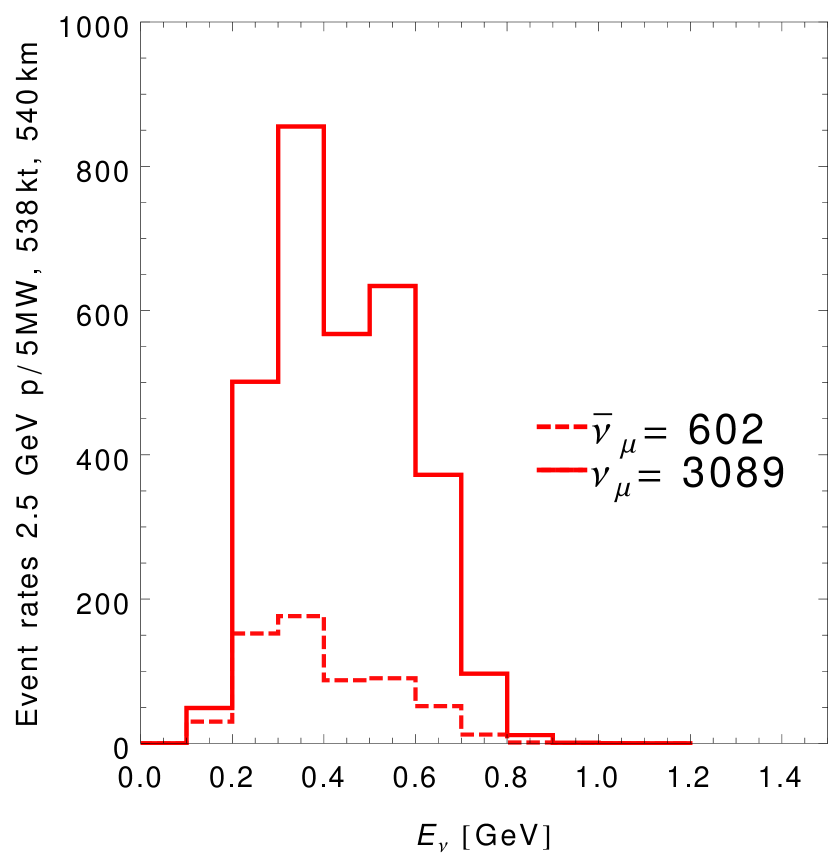
(a)

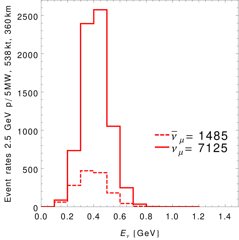
(b)

Figure 2: Expected muon-neutrino and antineutrino disappearance ($\nu_{\mu}/\bar{\nu}_{\mu}$) event rates per year for an ESS$\nu$SB setup using the neutrino oscillation parameters as given in Alekou et al. (2021), the left panel displays the baseline option of placing the detector at a distance of $L=$540 km and the right panel for $L=$360 km baseline case.

In Fig. 2, we display our expected signal events as a function of the neutrino energy, assuming one year of exposure, for both neutrinos and anti-neutrinos. The left panel is for the option of placing the detector at a baseline of 540 km from the source, and the right panel represents the baseline option at 360 km from the source.

Table 2: Our expected muon-neutrino disappearance signal and background events per year for an ESS$\nu$SB setup using the neutrino oscillation parameters as given in Alekou et al. (2021).

Baseline run	$\nu_{\mu}(\bar{\nu}_{\mu})$ sig.	$\bar{\nu}_{\mu}(\nu_{\mu})\rightarrow\bar{\nu}_{\mu}(\nu_{\mu})$	NC bckg.
360 km $\nu$	7125	54	87
$\leavevmode\nobreak\ \leavevmode\nobreak\ \leavevmode\nobreak\ \leavevmode\nobreak\ \leavevmode\nobreak\ \leavevmode\nobreak\ \leavevmode\nobreak\ \leavevmode\nobreak\ \leavevmode\nobreak\ \leavevmode\nobreak\ \leavevmode\nobreak\ (\bar{\nu}$)	1485	132	13
540 km $\nu$	3089	27	38
$\leavevmode\nobreak\ \leavevmode\nobreak\ \leavevmode\nobreak\ \leavevmode\nobreak\ \leavevmode\nobreak\ \leavevmode\nobreak\ \leavevmode\nobreak\ \leavevmode\nobreak\ \leavevmode\nobreak\ \leavevmode\nobreak\ \leavevmode\nobreak\ (\bar{\nu}$)	602	67	6

In Table 2, the total number of events per year for signal and background in the muon-neutrino disappearance channel is introduced for both neutrinos and antineutrinos. In our analysis, we consider only the $\bar{\nu}_{\mu}(\nu_{\mu})\rightarrow\bar{\nu}_{\mu}(\nu_{\mu})$ and $\nu_{\mu}(\bar{\nu}_{\mu})$ neutral current backgrounds for positive (negative) polarity, respectively, since they are the main contributions to this channel. As a result, there is essentially no background interference in the muon-neutrino disappearance channel.

IV.3 Scalar-field sensitivity

In this subsection, we introduce our results of the ULSF searches via neutrino oscillations at the ESS$\nu$SB from the combined analysis at both appearance and disappearance channels. We have already stated that the disappearance channel will give a more restrictive result for this kind of search due to its higher statistics. Still, we include in our analysis both the electron appearance as well as the muon disappearance channels, to be the most sensitive as possible.

We employ a chi-squared test to quantify the statistical significance of the ULSF sensitivity, which is given by the adding the two channels using both neutrino and anti-neutrino data sets. The $\chi^{2}$ function is given as

$$\chi^{2}=\sum_{\ell}\tilde{\chi}^{2}_{\ell}+\chi^{2}_{\text{prior}},$$ (20)

where the corresponding $\tilde{\chi}^{2}_{\ell}$ function for each channel $\ell=\{\nu_{\mu}(\bar{\nu}_{\mu})\rightarrow\nu_{e}(\bar{\nu}_{e}),\nu_{\mu}(\bar{\nu}_{\mu})\rightarrow\nu_{\mu}(\bar{\nu}_{\mu})\}$ in the large data size limit is given by

$$\tilde{\chi}^{2}_{\ell}=\min_{\xi_{j}}\Bigg{[}\sum_{i}^{n_{\text{bins}}}\frac{\big{(}N_{i,\text{true}}^{3\nu}-N_{i,\text{test}}^{3\nu+\eta}(\Omega,\eta,\{\xi_{j}\})\big{)}^{2}}{\sigma_{i,\text{true}}^{2}}+\sum_{j}^{n_{\text{syst.}}}\Big{(}\frac{\xi_{j}}{\sigma_{j}}\Big{)}^{2}\Bigg{]}.$$ (21)

The $N_{i}^{3\nu}$ are the simulated events at the $i$th energy bin considering the standard three neutrino oscillations as a true hypothesis. $N_{i}^{3\nu+\eta}$ are the computed events at the $i$th energy bin with the model assuming scalar field oscillations. $\Omega=\{\theta_{12},\theta_{13},\theta_{23},\delta,\Delta m_{21}^{2},\Delta m^{2}_{31}\}$ is the set of oscillation parameters, $\eta$ is the ULSF parameter and $\{\xi_{j}\}$ are the nuisance parameters to account for the signal, background normalization, and energy calibration systematics respectively. Moreover, $\sigma_{i}=\sqrt{N_{i}^{3\nu}}$ is the statistical error in each energy bin while $\sigma_{j}$ are the signal, background normalization, and energy calibration errors (see Sec. III). Furthermore, implementation of external input for the standard oscillation parameters on the $\chi^{2}$ function is performed via Gaussian priors

$$\chi^{2}_{\text{prior}}=\sum_{k}^{n_{\text{priors}}}\frac{\big{(}\Omega_{k,\text{true}}-\Omega_{k,\text{test}}\big{)}^{2}}{\sigma^{2}_{k}},$$ (22)

the central values of the priors $\Omega_{k}$ are set to their true or best-fit value for normal ordering de Salas et al. (2021). $\sigma_{k}$ is the uncertainty on the oscillation prior, which corresponds to a 1$\sigma$ error of $5\%$ for $\Delta m^{2}_{21}$, $\Delta m^{2}_{31}$, $\theta_{12}$, and $\theta_{23}$, $3\%$ for $\theta_{13}$, and $10\%$ for the leptonic $CP$-violating phase $\delta$ Baussan et al. (2014), the summation index $k$ runs over the corresponding test oscillation parameters to be marginalized.

Besides, the expected number of events at the $i$th energy bin is calculated as Huber et al. (2002)

$$N_{i}=\frac{\mathcal{N}}{L^{2}}\int^{E_{i}^{\prime}+\Delta E_{i}^{\prime}/2}_{E^{\prime}_{i}-\Delta E_{i}^{\prime}/2}dE^{\prime}\int^{\infty}_{0}dE\leavevmode\nobreak\ \Phi_{\nu}(E)\sigma_{\nu}(E)P_{\alpha\beta}(E)K(E,E^{\prime})\varepsilon(E^{\prime}),$$ (23)

where $E$ is the true neutrino energy, $E^{\prime}$ is the reconstructed neutrino energy, $\Delta E_{i}^{\prime}$ is the bin size of the $i$th energy bin, $\mathcal{N}$ is a constant normalization factor that accounts for the mass-year exposure and beam power, $L$ is the baseline distance, $\Phi_{\nu}(E)$ is the energy-dependent neutrino flux, $\sigma_{\nu}(E)$ is the energy-dependent cross section, $P_{\alpha\beta}(E)$ is the neutrino-oscillation probability, $K(E,E^{\prime})$ is the energy response-model or energy-resolution of the experiment, and $\varepsilon(E^{\prime})$ is the energy-dependent efficiency. Moreover, the neutrino-oscillation probability $P_{\alpha\beta}(E)=P_{\nu_{\alpha}\rightarrow\nu_{\beta}}(E,L,\rho,\theta_{12},\theta_{23},\theta_{13},\Delta m_{31}^{2},\Delta m_{21}^{2},\delta)$; the energy-resolution function, which relates the true and reconstructed neutrino energies follow a Gaussian distribution

$$K(E,E^{\prime})=\frac{1}{\sqrt{2\pi}\sigma_{R}(E)}\exp\Bigg{\{}-\frac{(E-E^{\prime})^{2}}{2\sigma_{R}^{2}(E)}\Bigg{\}},$$ (24)

where $\sigma_{R}(E)=\beta\sqrt{E/\text{GeV}}\leavevmode\nobreak\ \text{GeV}$, in our case we assume $\beta=(0.12,0.10)$ for ($e^{-},\mu^{-}$) respectively.

Furthermore, $N_{i}^{3\nu}=S^{3\nu}_{i}+B^{3\nu}_{i}$, $S_{i}^{3\nu}$, and $B_{i}^{3\nu}$ are the simulated signal and background events in each energy bin within the standard three neutrino oscillations framework, as described in Tables 1, and 2. They were computed according to Eq. (23) with true oscillation parameters fixed to their best-fit point for normal ordering (see Sec. IV.1). In addition, $N_{i}^{3\nu+\eta}=S^{3\nu+\eta}_{i}\big{(}1+\xi_{1}+g(E^{\prime})\xi_{3}\big{)}+B^{3\nu+\eta}_{i}\big{(}1+\xi_{2}+g(E^{\prime})\xi_{4}\big{)}$, $S_{i}^{3\nu+\eta}$, and $B_{i}^{3\nu+\eta}$ are the corresponding signal and background events in each energy bin, assuming the model with scalar field oscillations where $P_{\alpha\beta}(E)\rightarrow P_{\alpha\beta}(E,\eta)$. Likewise, the $\{\xi_{j}\}$ are the nuisance parameters describing the systematic errors, where $\xi_{1}$ and $\xi_{2}$ account for the signal and background normalization, respectively, whereas $\xi_{3}$ and $\xi_{4}$ account for the signal and background energy calibration, the energy calibration function $g(E^{\prime})$ is

$$g(E^{\prime})=\frac{(E_{i}^{\prime}-\bar{E}^{\prime})}{(E^{\prime}_{max}-E^{\prime}_{min})},$$ (25)

where $E_{i}^{\prime}$ is the mean reconstructed energy at the $i$th energy bin; $\bar{E}^{\prime}=\frac{1}{2}(E^{\prime}_{max}+E^{\prime}_{min})$ is the median of the energy interval, $E^{\prime}_{min}=0.1$ GeV is the minimum energy of the reconstructed energy window while $E^{\prime}_{max}=1.3$ GeV is the maximum energy of the reconstructed energy window.

The sensitivity contours were computed based on the $\Delta\chi^{2}=\chi^{2}-\chi^{2}_{\text{min}}$ distribution, scanning over the test parameter pairs, either ($\sin^{2}\theta_{23}$, $\eta$) or ($\Delta m^{2}_{31}$, $\eta$), with the ULSF parameter $\eta$ arising from the average modulation on the atmospheric mass-squared splitting $\Delta\tilde{m}_{31}^{2}$, as given in Eq. (17). All the remaining test oscillation parameters are marginalized over. The standard three neutrino oscillation picture is assumed as true hypothesis; the boundary of the corresponding allowed regions were determined by mapping the $\Delta\chi^{2}$ to corresponding confidence levels using a $\chi^{2}$-distribution, assuming Wilks theorem for two degrees of freedom.

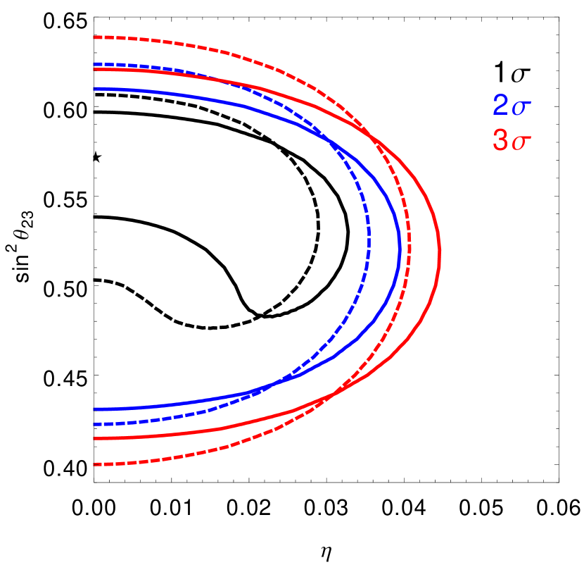
(a)

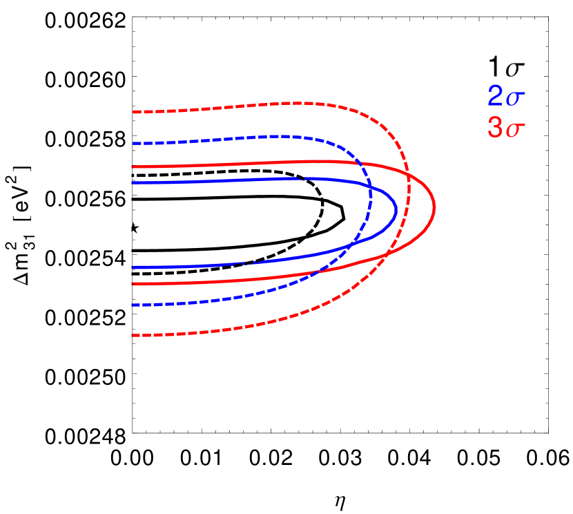
(b)

Figure 3: Expected sensitivity to the scalar field parameter $\eta$ from the atmospheric mass squared modulation at the ESS$\nu$SB setup; the baseline choice of $L=540$ km is shown in dashed lines, whereas the $L=360$ km in solid lines. The contours inside the black, blue, and red lines are the sensitivities at $1\sigma$, $2\sigma$, and $3\sigma$, respectively.

In Fig. 3, we show our sensitivities to the scalar field scenario. The left panel displays the expected sensitivity to the ULSF in the $(\eta,\sin^{2}\theta_{23})$ plane, whereas the right panel shows the expected sensitivity in the $(\eta,\Delta m^{2}_{31})$ plane, respectively. The contours inside the black, blue, and red lines are the sensitivities at ($1\sigma$, $2\sigma$, and $3\sigma$), which correspond to $\Delta\chi^{2}=$ (2.3, 6.18, and 11.83) accordingly. The star in the $\eta-\sin^{2}\theta_{23}$ and $\eta-\Delta m^{2}_{31}$ planes represent the best-fit point used in the simulated data under the true hypothesis. The solid lines assume an ESS$\nu$SB setup with a baseline of $L=360$ km, while the dashed lines represent a baseline of $L=540$ km.

We observe that the impact of the normalization systematic error is relevant for the $L=540$ km baseline, mainly due to a decrease in the signal events, spoiling the precision on the atmospheric mixing parameters, $\theta_{23}$ and $\Delta m^{2}_{31}$. However, the sensitivity to the scalar field parameter is not considerably affected. As a result, we anticipate a ULSF parameter sensitivity of $\eta<0.043\leavevmode\nobreak\ (0.039)$ at 3$\sigma$ and $\eta<0.032\leavevmode\nobreak\ (0.028)$ at 90$\%$ confidence limit (C.L.) i.e., $\Delta\chi^{2}=4.61$, at the $L=360$ km ($L=540$ km) baselines. Besides, the allowed values at $3\sigma$ for the mixing angle are $0.41\lesssim\sin^{2}\theta_{23}\lesssim 0.62$, and for the atmospheric mass-squared difference $2.53\times 10^{-3}\leavevmode\nobreak\ \text{eV}^{2}\lesssim\Delta m^{2}_{31}\lesssim 2.57\times 10^{-3}\leavevmode\nobreak\ \text{eV}^{2}$, at the $L=$ 360 km baseline option, while at the $L=$ 540 km baseline, the allowed values at $3\sigma$ are $0.40\lesssim\sin^{2}\theta_{23}\lesssim 0.64$ and $2.51\times 10^{-3}\leavevmode\nobreak\ \text{eV}^{2}\lesssim\Delta m^{2}_{31}\lesssim 2.59\times 10^{-3}\leavevmode\nobreak\ \text{eV}^{2}$.

We can notice the relevance of the expected sensitivity found here by comparing it with other studies for different types of neutrino physics. For instance, for solar neutrino experiments, it has been pointed out Berlin (2016) that an order $\mathcal{O}(10\%)$ anomalous modulation on the neutrino fluxes, due to an ultralight ($m_{\phi}\sim 10^{-22}$ eV) scalar coupling with neutrinos could happen at solar neutrino experiments. This result translates into a bound to the scalar field parameter of $\eta\sim 0.1$. In addition, a projected sensitivity of $\eta\sim 1.5\%$ and $\eta\sim 7.5\%$ via $\Delta m_{31}^{2}$ smearing are expected at the JUNO and DUNE experiments, respectively Krnjaic et al. (2018). Furthermore, bounds due to the modulations from the mass-squared splitting $\Delta m_{31}^{2}$ have been recently studied in Ref. Losada et al. (2022a), reporting a 1$\sigma$ sensitivity to the $\eta$ parameter for different neutrino experiments, such as Daya Bay; with a scalar field bound of $\eta\sim 0.08$ from the electron antineutrino disappearance channel. Similarly, the JUNO experiment is projected to be sensitive to $\eta\sim 0.005$, and from the electron neutrino appearance channel, a $\eta\sim 0.01$ bound is expected for both DUNE and Hyper-Kamiokande, respectively. Regarding DUNE, the authors of Ref. Dev et al. (2021) obtained a 1$\sigma$ sensitivity of $\eta\sim 0.035$. Hence, compared to our projected 1$\sigma$ sensitivities to the ULSF parameter at the ESS$\nu$SB setup of $\eta\sim 0.03$ from the $L=360$ km baseline option and $\eta\sim 0.027$ from the $L=540$ km baseline, competitive bounds on the ULSF parameter can be achieved. Consequently, we expect that with the inclusion of the muon-neutrino disappearance data set, we can motivate to extend the main physics program at the ESS$\nu$SB to search for this type of physics.

IV.4 Some cosmological implications of the neutrino-ULSF interaction

Before finishing this section, we would like to discuss some important characteristics and details of the scalar field in cosmology –they can be relevant when interpreting our results.

We start this subsection by noticing, as stated in Ref Berlin (2016), that the $\hat{y}\phi$ contribution in Eq. (9) will induce quantum corrections to the ULSF potential

$$V_{\phi}=\frac{m_{\phi}^{2}}{2}\phi^{2}+\hat{y}n_{\nu}\phi+\mathcal{O}(\hat{y}^{2})+\dots.$$ (26)

This contribution will produce a shift of the $\phi$ vacuum expectation value (VEV) that goes as $\hat{y}n_{\nu}\phi$, where $n_{\nu}$ is the neutrino number density. This shift could jeopardize the features of the ULSF as dark matter since the VEV of $\phi$ will be displaced at $T\sim$ GeV,

$$\langle-\phi\rangle\sim\frac{\hat{y}n_{\nu}}{m_{\phi}^{2}}\sim 10^{21}\leavevmode\nobreak\ \text{GeV}\leavevmode\nobreak\ \Big{(}\frac{\hat{y}}{10^{-40}}\Big{)}\Big{(}\frac{n_{\nu}}{0.1\text{GeV}^{3}}\Big{)}\Big{(}\frac{10^{-22}\text{eV}}{m_{\phi}}\Big{)}.$$ (27)

For this reason, it is important to consider that the temperature associated with the phase transition that sets the initial conditions for the ULSF field it is well below $1$ MeV Berlin (2016).

If $\phi$ begins to oscillate at $T_{\text{osc}}\sim\sqrt{M_{\text{Pl}}m_{\phi}}\leavevmode\nobreak\ (m_{\phi}/10^{-22}\text{eV})\sim$ keV Hui et al. (2017), around this temperature, the redshift $z_{\text{osc}}\sim 2\times 10^{6}$ and the average density $\rho_{\phi}(z)\sim 10^{-5}\rho_{\phi,\odot}(1+z)^{3}$. Thus, the scalar-field amplitude $\phi_{\text{keV}}(z=2\times 10^{6})\simeq 10^{26}$ eV $\simeq 10^{17}$ GeV. From the sensitivity to the ULSF parameter $\eta\sim$ 0.01 at ESS$\nu$SB, using Eq. (14) we obtain $\hat{y}\sim 10^{-23}\leavevmode\nobreak\ (m_{\phi}/10^{-22}\text{eV})$ at present time. However if the coupling $\hat{y}$ remains unmodified back to the oscillation temperature, the VEV of the scalar field ($\langle-\phi\rangle=\phi_{\text{min}}$) is

$$\langle-\phi\rangle\sim\frac{\hat{y}n_{\nu}}{m_{\phi}^{2}}\sim 10^{20}\leavevmode\nobreak\ \text{GeV}\leavevmode\nobreak\ \Big{(}\frac{\hat{y}}{10^{-23}}\Big{)}\Big{(}\frac{n_{\nu}}{10^{-19}\text{GeV}^{3}}\Big{)}\Big{(}\frac{10^{-22}\text{eV}}{m_{\phi}}\Big{)},$$ (28)

thus, $\phi_{\text{min}}\sim 10^{3}$ $\phi_{\text{keV}}$ (which requires a coupling $\hat{y}\lesssim 10^{-27}\leavevmode\nobreak\ (m_{\phi}/10^{-22}\text{eV})$ to avoid large corrections to the neutrino mass, well below the sensitivity of any terrestrial neutrino oscillation experiment). Furthermore, the contributions to the neutrino mass are $\hat{y}\phi_{\text{keV}}\simeq 10^{3}$ eV and $\hat{y}\phi_{\text{min}}\simeq 10^{6}$ eV, hence the effective neutrino mass at this temperature would be $\tilde{m}(t)\simeq 10^{6}$ eV.

On the other hand, around matter-radiation equality where $T_{\text{eq}}\sim 1$ eV; the potential $\hat{y}\phi\sim 10^{-23}\times 10^{22}$ eV $\sim 0.1$ eV and $\hat{y}(\phi+\phi_{\text{min}})\sim 0.11$ eV. Besides, the effective neutrino mass $\tilde{m}(t)\simeq m_{\nu}+\hat{y}(\phi+\phi_{\text{min}})$, assuming a bare neutrino mass $m_{\nu}\sim 0.1$ eV we obtain $\tilde{m}(t)\simeq 0.21$ eV, which is within the limit of the CMB constraint $\sum_{i}m_{i}<0.23$ eV Ade et al. (2016). Therefore, without invoking any model realization, unless the temperature associated with the phase transition of the ULSF occurs after matter-radiation equality (say at $T\sim m_{\nu}\sim 0.1$ eV), strong constraints apply to the neutrino-ULDM scenario at ESS$\nu$SB. Moreover, if this transition happens after the formation of the CMB, the ULSF can only constitute a fraction of the DM Krnjaic et al. (2018). Therefore, in our analysis for the ESS$\nu$SB, we can consider the scalar field as being a component of the dark matter, or to be just an ultralight scalar field without participating of the DM components Capozzi:2018bps .

In the case that the phase transition can happen at temperatures of the order of $10$ MeV, there could be potential contributions to the effective number of neutrino species $N_{\text{eff}}$ during big bang nucleosynthesis (BBN). In this scenario, the interaction term $\hat{y}\phi$ could increase $N_{\text{eff}}$ during BBN. However, the density of thermal neutrinos may have dominated the ULSF potential throughout this epoch, modifying Eqs. (5) and (6).

For instance, within the scenario of active-sterile mixing Huang et al. (2022) where $\hat{y}\approx\sin^{2}\theta g$, a potential $g\phi_{\odot}\sim 10^{-7}$ eV $(g/10^{-22})(10^{-18}\text{eV}/m_{\phi})$ is able to maintain $\Delta N_{\text{eff}}\lesssim 10^{-2}$, increasing the potential will further reduce the contribution to $\Delta{N}_{\text{eff}}$. From the sensitivity to the ULSF parameter $\eta\sim$ 0.01 at ESS$\nu$SB, we obtain a similar potential $g\phi_{\odot}\sim 10^{-7}$ eV $(\hat{y}/10^{-23})(0.1/\sin^{2}\theta)(10^{-18}\text{eV}/m_{\phi})$. Therefore, we do not expect a restriction from BBN in this scenario. Other constraints from BBN can be found in Refs. Blinov et al. (2019); Dev et al. (2022); Huang et al. (2018); Venzor et al. (2021).

On the other hand, the CMB observations constrain the sum of the neutrino masses $\sum_{i}m_{i}\lesssim 0.23$ eV Ade et al. (2016); for modulations via $\Delta m_{31}^{2}$, according to Krnjaic et al. (2018), this implies $\eta(z=0)\lesssim 9\times 10^{-3}\leavevmode\nobreak\ (m_{\phi}/10^{-22}\text{eV})$, which is in good agreement with the ESS$\nu$SB sensitivity, $\eta(z=0)\lesssim 0.01$.

Within the CMB era, there could be an important case to consider for us. If the potential $\hat{y}\phi$ dominates over the neutrino bare mass terms, the neutrino mass will significantly change. The relevant neutrino mass states $\nu_{1},\nu_{3}$ will have the contribution Berlin (2016)

$$m_{1,3}(t)\simeq\hat{y}_{1,3}\langle\phi\rangle\simeq\frac{2\hat{y}_{1,3}\sqrt{2\rho_{\phi}}}{\pi m_{\phi}}.$$ (29)

The CMB bound on the neutrino masses implies a restriction for the coupling, $\hat{y}_{1,3}^{\text{CMB}}(z=0)\lesssim 6\times 10^{-21}\leavevmode\nobreak\ (m_{\phi}/10^{-22}\text{eV})$. As we have mentioned, ESS$\nu$SB will be sensitive to the phenomenological parameter $\eta$ [Eq. (14)] at the percent level,

$$\eta_{\Delta}\propto\hat{y}_{i}\sqrt{\rho_{\phi}}/m_{\phi}.$$ (30)

This means that, for our usual choice of values $m_{\phi}$ and $\rho_{\phi}$, the sensitivity to the coupling $\hat{y}_{1,3}^{\text{CMB}}(z=0)$ would be at least one order of magnitude smaller than the ESS$\nu$SB sensitivity.

The previous discussions assume that the ULSF accounts for all the DM in the Universe ($\rho_{\phi}=\rho_{\text{DM},\odot}$). This may not be the case, and the ULSF could be only a fraction of this DM. The main phenomenological parameter, $\eta$, includes the DM density and would imply that $\hat{y}_{1,3}\propto\eta/\sqrt{\rho_{\phi}}$, if the $\phi$ accounts for less than 20$\%$ of the total DM density Kobayashi et al. (2017); the scalar field amplitude $\phi_{0}$ decreases by a factor of two, thus the coupling $\hat{y}_{1,3}\gtrsim 2\times 10^{-23}\leavevmode\nobreak\ (\eta/0.01)(m_{\phi}/10^{-22}\leavevmode\nobreak\ \text{eV})$. Therefore, in this scenario, the sensitivity to $\hat{y}_{1,3}$ will be weaker. On the other hand, for the local DM density $\rho_{\text{DM},\odot}\simeq 0.3-0.6\leavevmode\nobreak\ \text{GeV/cm}^{3}$; for $\rho_{\phi}=\rho_{\text{DM},\odot}$, the coupling can vary between the range $\hat{y}_{1,3}\simeq\big{[}1/\sqrt{2}-1\big{]}\times 10^{-23}\leavevmode\nobreak\ (\eta/0.01)(m_{\phi}/10^{-22}\text{eV})$.

Notice that, since $\hat{y}_{1,3}\propto\eta m_{\phi}$, a larger ULSF mass will reduce the sensitivity on the coupling $\hat{y}_{1,3}$ for fixed density $\rho_{\phi}$. However, most observational features of a ULSF as DM favor a mass range $m_{\phi}\sim(10^{-1}-10)\times 10^{-22}$ eV Urena-Lopez (2007); Ureña López (2019); Rodriguez-Montoya et al. (2010); Arbey et al. (2002); Lesgourgues et al. (2002); Arbey et al. (2003); Matos and Urena-Lopez (2000); Matos et al. (2009); Arbey et al. (2001); Matos and Urena-Lopez (2001); Suarez and Matos (2011); Magana and Matos (2012); Suárez et al. (2014); Hui et al. (2017).

Finally, we might worry about the thermalization of the ULSF at distant past via $\nu\phi\rightarrow\nu\phi$ scatterings, which can lead to equilibrium among neutrinos and the ULSF. Nevertheless, the elastic scattering cross section for a scalar self-conjugate field, such as the ULSF with active neutrinos, via a spin one-half fermion $N$ ($M_{N}\gg m_{\phi}$) exchange is zero Boehm and Fayet (2004).

V Conclusions

The dark matter problem is one of the main puzzles in physics, and different solutions have been proposed over the years. The existence of dark matter has been a strong motivation to explore alternative physical models and interactions to understand all its physical consequences ranging from particle physics to cosmology. In particular, the scalar field dark matter proposal is very successful at the cosmological level and deserves further exploration of its possible interactions with a Standard Model particle.

In this paper, we have discussed in detail the implications of a hypothetical interaction between neutrinos and an ULSF, as well as the case were this field is a DM candidate. We focused in the case of the long-baseline neutrino experiment at the ESS$\nu$SB. As already discussed, a broad set of proposals considers either modifying of gravitational interactions or new particles at different mass scales. We have focused on the case of an ultralight scalar field and its hypothetical interaction with neutrinos. In this scenario, a modification in the expected oscillation pattern in long baseline neutrinos is expected. This modification could affect either the-neutrino mixing angles or mass-squared differences. The ESS$\nu$SB is sensitive to the ULSF via modulations on the atmospheric mass squared difference $\Delta m_{31}^{2}$.

We found that sensitivities to the main parameter modeling the interaction between the ULSF and neutrinos are: $\eta<0.043\leavevmode\nobreak\ (0.039)$ at 3$\sigma$ and $\eta<0.032\leavevmode\nobreak\ (0.028)$ at 90$\%$ C.L., from the $L=360$ km and ($L=540$ km) baselines, respectively. Our bounds are comparable to other long-baseline searches of this parameter. For instance, in Ref. Krnjaic et al. (2018), a projected sensitivity of $\eta\sim 1.5\%$ and $\eta\sim 7.5\%$ via $\Delta m_{31}^{2}$ smearing are expected at JUNO and DUNE experiments, respectively. Projected 1$\sigma$ sensitivities of $\eta\sim 0.035$ at DUNE Dev et al. (2021) and $\eta\sim 0.01$ Losada et al. (2022a) at both DUNE and Hyper-Kamiokande were also reported in the literature. Regarding reactor neutrino experiments, 1$\sigma$ sensitivities of $\eta\sim 0.08$ from Daya Bay and $\eta\sim 0.005$ from JUNO are reported Losada et al. (2022a). All these bounds are comparable to our 1$\sigma$ sensitivities to the ULSF parameter at the ESS$\nu$SB setup, namely $\eta\sim 0.03$ from the $L=360$ km baseline option and $\eta\sim 0.027$ from the $L=540$ km baseline. Therefore, the incorporation of the muon-neutrino disappearance sample will not only benefit precision measurements at ESS$\nu$SB Alekou et al. (2021) but also opens a window to search for scalar-field modulations from the atmospheric mass-squared splitting $\Delta m_{31}^{2}$.

The ESS$\nu$SB experiment represents an opportunity to measure the leptonic $CP$-violating phase accurately. Besides, it will allow searching for different types of new physics at a competitive level. The case of the ULSF candidate is an example of this potential.

References

- Sahni and Wang (2000) V. Sahni and L.-M. Wang, Phys. Rev. D 62, 103517 (2000), eprint astro-ph/9910097.
- Hu et al. (2000) W. Hu, R. Barkana, and A. Gruzinov, Phys. Rev. Lett. 85, 1158 (2000), eprint astro-ph/0003365.
- Matos et al. (2000) T. Matos, F. S. Guzman, and L. A. Urena-Lopez, Class. Quant. Grav. 17, 1707 (2000), eprint astro-ph/9908152.
- Matos and Urena-Lopez (2000) T. Matos and L. A. Urena-Lopez, Class. Quant. Grav. 17, L75 (2000), eprint astro-ph/0004332.
- Arbey et al. (2002) A. Arbey, J. Lesgourgues, and P. Salati, Phys. Rev. D 65, 083514 (2002), eprint astro-ph/0112324.
- Arbey et al. (2001) A. Arbey, J. Lesgourgues, and P. Salati, Phys. Rev. D 64, 123528 (2001), eprint astro-ph/0105564.
- Magana and Matos (2012) J. Magana and T. Matos, J. Phys. Conf. Ser. 378, 012012 (2012), eprint 1201.6107.
- Suárez et al. (2014) A. Suárez, V. H. Robles, and T. Matos, Astrophys. Space Sci. Proc. 38, 107 (2014), eprint 1302.0903.
- Marsh (2016) D. J. E. Marsh, Phys. Rept. 643, 1 (2016), eprint 1510.07633.
- Hui et al. (2017) L. Hui, J. P. Ostriker, S. Tremaine, and E. Witten, Phys. Rev. D 95, 043541 (2017), eprint 1610.08297.
- Lee (2018) J.-W. Lee, EPJ Web Conf. 168, 06005 (2018), eprint 1704.05057.
- Ureña López (2019) L. A. Ureña López, Front. Astron. Space Sci. 6, 47 (2019).
- Matos et al. (2009) T. Matos, A. Vazquez-Gonzalez, and J. Magana, Mon. Not. Roy. Astron. Soc. 393, 1359 (2009), eprint 0806.0683.
- Rodriguez-Montoya et al. (2010) I. Rodriguez-Montoya, J. Magana, T. Matos, and A. Perez-Lorenzana, Astrophys. J. 721, 1509 (2010), eprint 0908.0054.
- Lesgourgues et al. (2002) J. Lesgourgues, A. Arbey, and P. Salati, New Astron. Rev. 46, 791 (2002).
- Arbey et al. (2003) A. Arbey, J. Lesgourgues, and P. Salati, Phys. Rev. D 68, 023511 (2003), eprint astro-ph/0301533.
- Harko (2011) T. Harko, Mon. Not. Roy. Astron. Soc. 413, 3095 (2011), eprint 1101.3655.
- Robles and Matos (2012) V. H. Robles and T. Matos, Mon. Not. Roy. Astron. Soc. 422, 282 (2012), eprint 1201.3032.
- Lee and Lim (2010) J.-W. Lee and S. Lim, JCAP 01, 007 (2010), eprint 0812.1342.
- Berlin (2016) A. Berlin, Phys. Rev. Lett. 117, 231801 (2016), eprint 1608.01307.
- Brdar et al. (2018) V. Brdar, J. Kopp, J. Liu, P. Prass, and X.-P. Wang, Phys. Rev. D 97, 043001 (2018), eprint 1705.09455.
- Krnjaic et al. (2018) G. Krnjaic, P. A. N. Machado, and L. Necib, Phys. Rev. D 97, 075017 (2018), eprint 1705.06740.
- Liao et al. (2018) J. Liao, D. Marfatia, and K. Whisnant, JHEP 04, 136 (2018), eprint 1803.01773.
- Kim et al. (2020) D. Kim, P. A. N. Machado, J.-C. Park, and S. Shin, JHEP 07, 057 (2020), eprint 2003.07369.
- Dev et al. (2021) A. Dev, P. A. N. Machado, and P. Martínez-Miravé, JHEP 01, 094 (2021), eprint 2007.03590.
- Losada et al. (2022a) M. Losada, Y. Nir, G. Perez, and Y. Shpilman, JHEP 04, 030 (2022a), eprint 2107.10865.
- Zhao (2017) Y. Zhao, Phys. Rev. D 95, 115002 (2017), eprint 1701.02735.
- Farzan (2019) Y. Farzan, Phys. Lett. B 797, 134911 (2019), eprint 1907.04271.
- Cline (2020) J. M. Cline, Phys. Lett. B 802, 135182 (2020), eprint 1908.02278.
- Dev et al. (2022) A. Dev, G. Krnjaic, P. Machado, and H. Ramani (2022), eprint 2205.06821.
- Huang et al. (2022) G.-y. Huang, M. Lindner, P. Martínez-Miravé, and M. Sen, Phys. Rev. D 106, 033004 (2022), eprint 2205.08431.
- Losada et al. (2022b) M. Losada, Y. Nir, G. Perez, I. Savoray, and Y. Shpilman (2022b), eprint 2205.09769.
- Kobayashi et al. (2017) T. Kobayashi, R. Murgia, A. De Simone, V. Iršič, and M. Viel, Phys. Rev. D 96, 123514 (2017), eprint 1708.00015.
- (34) N. Bar, K. Blum and C. Sun, Phys. Rev. D 105, no.8, 8 (2022), eprint 2111.03070.
- Baussan et al. (2014) E. Baussan et al. (ESSnuSB), Nucl. Phys. B 885, 127 (2014), eprint 1309.7022.
- Alekou et al. (2021) A. Alekou et al. (ESSnuSB), Eur. Phys. J. C 81, 1130 (2021), eprint 2107.07585.
- Alekou et al. (2022) A. Alekou et al. (2022), eprint 2206.01208.
- Agostino et al. (2013) L. Agostino, M. Buizza-Avanzini, M. Dracos, D. Duchesneau, M. Marafini, M. Mezzetto, L. Mosca, T. Patzak, A. Tonazzo, and N. Vassilopoulos (MEMPHYS), JCAP 01, 024 (2013), eprint 1206.6665.
- Kumar Agarwalla et al. (2019) S. Kumar Agarwalla, S. S. Chatterjee, and A. Palazzo, JHEP 12, 174 (2019), eprint 1909.13746.
- Ghosh et al. (2020) M. Ghosh, T. Ohlsson, and S. Rosauro-Alcaraz, JHEP 03, 026 (2020), eprint 1912.10010.
- Choubey et al. (2021) S. Choubey, M. Ghosh, D. Kempe, and T. Ohlsson, JHEP 05, 133 (2021), eprint 2010.16334.
- Majhi et al. (2021) R. Majhi, D. K. Singha, K. N. Deepthi, and R. Mohanta, Phys. Rev. D 104, 055002 (2021), eprint 2101.08202.
- Blennow et al. (2020a) M. Blennow, M. Ghosh, T. Ohlsson, and A. Titov, JHEP 07, 014 (2020a), eprint 2004.00017.
- Chatterjee et al. (2021) S. S. Chatterjee, O. G. Miranda, M. Tórtola, and J. W. F. Valle (2021), eprint 2111.08673.
- Ahn et al. (2022) Y. H. Ahn, S. K. Kang, R. Ramos, and M. Tanimoto (2022), eprint 2205.02796.
- Huber et al. (2005) P. Huber, M. Lindner, and W. Winter, Comput. Phys. Commun. 167, 195 (2005), eprint hep-ph/0407333.
- Huber et al. (2007) P. Huber, J. Kopp, M. Lindner, M. Rolinec, and W. Winter, Comput. Phys. Commun. 177, 432 (2007), eprint hep-ph/0701187.
- Carr and Kuhnel (2020) B. Carr and F. Kuhnel, Ann. Rev. Nucl. Part. Sci. 70, 355 (2020), eprint 2006.02838.
- Carr et al. (2021) B. Carr, F. Kuhnel, and L. Visinelli, Mon. Not. Roy. Astron. Soc. 506, 3648 (2021), eprint 2011.01930.
- Arbey and Mahmoudi (2021) A. Arbey and F. Mahmoudi, Prog. Part. Nucl. Phys. 119, 103865 (2021), eprint 2104.11488.
- Di Luzio et al. (2020) L. Di Luzio, M. Giannotti, E. Nardi, and L. Visinelli, Phys. Rept. 870, 1 (2020), eprint 2003.01100.
- Arun et al. (2017) K. Arun, S. B. Gudennavar, and C. Sivaram, Adv. Space Res. 60, 166 (2017), eprint 1704.06155.
- Drewes (2013) M. Drewes, Int. J. Mod. Phys. E 22, 1330019 (2013), eprint 1303.6912.
- Ng et al. (2019) K. C. Y. Ng, B. M. Roach, K. Perez, J. F. Beacom, S. Horiuchi, R. Krivonos, and D. R. Wik, Phys. Rev. D 99, 083005 (2019), eprint 1901.01262.
- Oks (2021) E. Oks, New Astron. Rev. 93, 101632 (2021), eprint 2111.00363.
- Milgrom (1983) M. Milgrom, Astrophys. J. 270, 365 (1983).
- Baker et al. (2021) T. Baker et al., Rev. Mod. Phys. 93, 015003 (2021), eprint 1908.03430.
- Randall and Sundrum (1999a) L. Randall and R. Sundrum, Phys. Rev. Lett. 83, 3370 (1999a), eprint hep-ph/9905221.
- Randall and Sundrum (1999b) L. Randall and R. Sundrum, Phys. Rev. Lett. 83, 4690 (1999b), eprint hep-th/9906064.
- Clowe et al. (2006) D. Clowe, M. Bradac, A. H. Gonzalez, M. Markevitch, S. W. Randall, C. Jones, and D. Zaritsky, Astrophys. J. Lett. 648, L109 (2006), eprint astro-ph/0608407.
- Klypin et al. (1999) A. A. Klypin, A. V. Kravtsov, O. Valenzuela, and F. Prada, Astrophys. J. 522, 82 (1999), eprint astro-ph/9901240.
- Moore et al. (1999) B. Moore, S. Ghigna, F. Governato, G. Lake, T. R. Quinn, J. Stadel, and P. Tozzi, Astrophys. J. Lett. 524, L19 (1999), eprint astro-ph/9907411.
- Peebles and Nusser (2010) P. J. E. Peebles and A. Nusser, Nature 465, 565 (2010), eprint 1001.1484.
- Lundgren et al. (2010) A. P. Lundgren, M. Bondarescu, R. Bondarescu, and J. Balakrishna, Astrophys. J. Lett. 715, L35 (2010), eprint 1001.0051.
- Matos and Urena-Lopez (2001) T. Matos and L. A. Urena-Lopez, Phys. Rev. D 63, 063506 (2001), eprint astro-ph/0006024.
- Suarez and Matos (2011) A. Suarez and T. Matos, Mon. Not. Roy. Astron. Soc. 416, 87 (2011), eprint 1101.4039.
- Arvanitaki et al. (2010) A. Arvanitaki, S. Dimopoulos, S. Dubovsky, N. Kaloper, and J. March-Russell, Phys. Rev. D 81, 123530 (2010), eprint 0905.4720.
- Cicoli et al. (2022) M. Cicoli, V. Guidetti, N. Righi, and A. Westphal, JHEP 05, 107 (2022), eprint 2110.02964.
- Bernal et al. (2018) T. Bernal, L. M. Fernández-Hernández, T. Matos, and M. A. Rodríguez-Meza, Mon. Not. Roy. Astron. Soc. 475, 1447 (2018), eprint 1701.00912.
- Ureña López et al. (2017) L. A. Ureña López, V. H. Robles, and T. Matos, Phys. Rev. D 96, 043005 (2017), eprint 1702.05103.
- Hlozek et al. (2015) R. Hlozek, D. Grin, D. J. E. Marsh, and P. G. Ferreira, Phys. Rev. D 91, 103512 (2015), eprint 1410.2896.
- (72) N. Bar, D. Blas, K. Blum and S. Sibiryakov, Phys. Rev. D 98, no.8, 083027 (2018), eprint 1805.00122.
- Arvanitaki et al. (2015) A. Arvanitaki, J. Huang, and K. Van Tilburg, Phys. Rev. D 91, 015015 (2015), eprint 1405.2925.
- Urena-Lopez (2007) L. A. Urena-Lopez, in 4th Mexican School of Astrophysics (2007), pp. 295–302.
- de Salas et al. (2019) P. F. de Salas, K. Malhan, K. Freese, K. Hattori, and M. Valluri, JCAP 10, 037 (2019), eprint 1906.06133.
- de Salas and Widmark (2021) P. F. de Salas and A. Widmark, Rept. Prog. Phys. 84, 104901 (2021), eprint 2012.11477.
- Sivertsson et al. (2022) S. Sivertsson, J. I. Read, H. Silverwood, P. F. de Salas, K. Malhan, A. Widmark, C. F. P. Laporte, S. Garbari, and K. Freese, Mon. Not. Roy. Astron. Soc. 511, 1977 (2022), eprint 2201.01822.
- Campagne et al. (2007) J.-E. Campagne, M. Maltoni, M. Mezzetto, and T. Schwetz, JHEP 04, 003 (2007), eprint hep-ph/0603172.
- Blennow et al. (2020b) M. Blennow, E. Fernandez-Martinez, T. Ota, and S. Rosauro-Alcaraz, Eur. Phys. J. C 80, 190 (2020b), eprint 1912.04309.
- Nunokawa et al. (2008) H. Nunokawa, S. J. Parke, and J. W. F. Valle, Prog. Part. Nucl. Phys. 60, 338 (2008), eprint 0710.0554.
- de Salas et al. (2021) P. F. de Salas, D. V. Forero, S. Gariazzo, P. Martínez-Miravé, O. Mena, C. A. Ternes, M. Tórtola, and J. W. F. Valle, JHEP 02, 071 (2021), eprint 2006.11237.
- Esteban et al. (2020) I. Esteban, M. C. Gonzalez-Garcia, M. Maltoni, T. Schwetz, and A. Zhou, JHEP 09, 178 (2020), eprint 2007.14792.
- Agarwalla et al. (2014) S. K. Agarwalla, S. Choubey, and S. Prakash, JHEP 12, 020 (2014), eprint 1406.2219.
- Chakraborty et al. (2019) K. Chakraborty, S. Goswami, C. Gupta, and T. Thakore, JHEP 05, 137 (2019), eprint 1902.02963.
- Choubey and Roy (2006) S. Choubey and P. Roy, Phys. Rev. D 73, 013006 (2006), eprint hep-ph/0509197.
- Huber et al. (2002) P. Huber, M. Lindner, and W. Winter, Nucl. Phys. B 645, 3 (2002), eprint hep-ph/0204352.
- Ade et al. (2016) P. A. R. Ade et al. (Planck), Astron. Astrophys. 594, A13 (2016), eprint 1502.01589.
- (88) F. Capozzi, I. M. Shoemaker and L. Vecchi, JCAP 07, 004 (2018), eprint 1804.05117.
- Blinov et al. (2019) N. Blinov, K. J. Kelly, G. Z. Krnjaic, and S. D. McDermott, Phys. Rev. Lett. 123, 191102 (2019), eprint 1905.02727.
- Huang et al. (2018) G.-y. Huang, T. Ohlsson, and S. Zhou, Phys. Rev. D 97, 075009 (2018), eprint 1712.04792.
- Venzor et al. (2021) J. Venzor, A. Pérez-Lorenzana, and J. De-Santiago, Phys. Rev. D 103, 043534 (2021), eprint 2009.08104.
- Lorenz et al. (2021) C. S. Lorenz, L. Funcke, M. Löffler, and E. Calabrese, Phys. Rev. D 104, 123518 (2021), eprint 2102.13618.
- Boehm and Fayet (2004) C. Boehm and P. Fayet, Nucl. Phys. B 683, 219 (2004), eprint hep-ph/0305261.