[figure]style=plain,subcapbesideposition=top plaintop table

Non-Markovian modeling of non-equilibrium fluctuations and dissipation in active viscoelastic biomatter

Abstract

Based on a Hamiltonian that incorporates the elastic coupling between a tracer and active particles, we derive a generalized Langevin model for the non-equilibrium mechanical response of active viscoelastic biomatter. Our model accounts for the power-law viscoelastic response of the embedding polymeric network as well as for the non-equilibrium energy transfer between active and tracer particles. Our analytical expressions for the frequency-dependent response function and the positional autocorrelation function agree nicely with experimental data for red blood cells and actomyosin networks with and without ATP. The fitted effective active-particle temperature, elastic constants and effective friction coefficients of our model allow straightforward physical interpretation.

Viscoelastic gels such as permanently or transiently cross-linked networks of semiflexible polymers are important soft biological materials [1, 2, 3]. The polymeric nature of such gels is responsible for their salient rheological properties, including their frequency-dependent response to external forces. The cell cytoskeleton is a prime example of a viscoelastic gel [4, 5] and determines cell shape, motility and division [6, 7]. Even though the cytoskeleton has a complex structure, its mechanical properties at small deformations are determined mainly by the underlying F-actin network [8, 9]. Even in equilibrium, the dynamic properties of F-actin are complex and interesting [10]. In vivo, constant F-actin (de)polymerization and interactions with myosin motors consume naturally occurring adenosine-tri-phosphate (ATP) and drive the viscoelastic network into a non-equilibrium (NEQ) state [11, 12, 13], where the motors act as active cross-links and produce local tension [2].

Another illustrious example of active viscoelastic biomatter are red blood cells (RBCs), whose structural components include a filamentous protein (spectrin) scaffold underneath the enclosing cell membrane [14, 15, 16, 17, 18]. The mechanical response and spectra of membrane fluctuations (RBC flickering) display active NEQ signatures that are attributed to the membrane ion-pump activity and the ATP-induced reorganization of the spectrin network [19, 20, 21].

Supported by high-resolution experimental data [22, 13, 23, 24, 20, 25, 26, 18], a key line of inquiry has been to examine violations of the fluctuation-dissipation theorem (FDT) in these NEQ systems. The FDT holds for near-equilibrium (near-EQ) dynamical processes, but not for active NEQ processes, as indeed corroborated by microrheology experiments [13, 20]. Typical experiments involve a micron-sized tracer bead immersed in the active medium whose motion is tracked and which is either allowed to move spontaneously or is driven by a laser beam (passive versus active microrheology). Active microrheology allows to simultaneously measure the mechanical-response and the positional autocorrelation function and thereby to check the validity of the FDT.

Theoretical studies of FDT violation focused on externally forced systems [27, 28, 29], glasses [30] and active systems [13, 20, 31]. In a generalized approach based on the Langevin equation, NEQ fluctuations have been modeled by an additive athermal noise acting on particles in a viscous fluid [21, 32]. A similar strategy has been used to model active dynamical undulations of elastic biological membranes [33, 21, 34, 35] and several computational models have explicitly incorporated active pumps [20, 36]. A non-equilibrium multicomponent elastic model for the interaction of motors and a tracer particle was recently shown to describe the frequency-dependence of the experimentally observed FDT violation [13] rather well [37].

In this paper, we model the non-equilibrium mechanical response in active biomatter by taking into account the medium viscoelasticity and the elastic coupling between tracer and the active particles. We derive analytical expressions for mechanical-response and spatial correlation functions, by simultaneously fitting these functions to experimental microrheological data for RBCs [20] and reconstituted actomyosin networks [13] we extract all parameters describing the viscoelastic medium and the elastic coupling between tracer and active particles. We find that power-law viscoelasticity describes the experimental data better than the standard Maxwell and Kelvin-Voigt viscoelastic models. The extracted viscoelastic exponent is close to $\kappa=3/4$ for actomyosin networks and close to unity for RBC, in agreement with previous studies. Interestingly, in the presence of ATP the effective temperature ratio between active and tracer particles is above 20 for both systems, demonstrating that these systems are very far from equilibrium. Our analysis and the quantitative agreement established with experiments demonstrates the generic capability of our multicomponent elastic model and our hybrid approach that combines relevant particle-based and hydrodynamic aspects of the problem into a single framework and enables closed-form predictions.

Table 1: Model parameters obtained from fits to the experimental data

Exp.	$\kappa$	$\gamma[\text{pN.s}^{\kappa}/\mu\text{m}]$	$K[\text{pN}/\mu\text{m}]$	$\hat{k}[\text{pN}/\mu\text{m}]$	$\hat{\gamma}_{\text{a}}[\text{pN.s}^{\kappa}/\mu\text{m}]$	$\alpha$
RBC:
EQ	$0.926\pm 0.0655$	$0.120\pm 0.00295$	$5.51\pm 0.109$	$1.31\pm 0.137$	$0.257\pm 0.0219$	$0.985\pm 0.197$
NEQ	$0.939\pm 0.0596$	$0.0749\pm 0.00164$	$1.66\pm 0.0289$	$0.283\pm 0.0361$	$0.155\pm 0.0186$	$36.3\pm 4.76$
ACM:
EQ	$0.737\pm 0.0388$	$6.053\pm 0.785$	$90.5\pm 4.30$	$40.3\pm 4.28$	$41.1\pm 7.26$	$-0.035\pm 0.144$
NEQ	$0.731\pm 0.0616$	$7.082\pm 0.891$	$189.0\pm 8.65$	$98.5\pm 13.6$	$61.9\pm 6.07$	$23.37\pm 2.83$

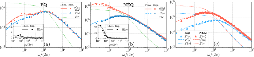
Figure 1: RBC flickering. Comparison of experimental data (symbols) [20] and our model predictions for the positional autocorrelation function $\omega\tilde{C}(\omega)/(2k_{\text{B}}T)$ in Eq. (Non-Markovian modeling of non-equilibrium fluctuations and dissipation in active viscoelastic biomatter) (solid lines) and the imaginary part of the response function $\tilde{\chi}^{\prime\prime}(\omega)$ Eq. (Non-Markovian modeling of non-equilibrium fluctuations and dissipation in active viscoelastic biomatter) (broken lines) for (a) the EQ scenario, i.e. ATP-depleted RBCs, and (b) the NEQ scenario, i.e. RBCs in the presence of ATP. In the insets, the spectral function $\Xi(\omega)$ from the experiments (symbols) is compared with our analytical prediction Eq. (10). (c) Comparison of the real and imaginary parts of the response function $\tilde{\chi}^{\prime}(\omega)$ and $\tilde{\chi}^{\prime\prime}(\omega)$ for the NEQ and EQ scenarios, indicating a larger response (i.e. a softening and less dissipation) in the NEQ case in particular at low frequencies. The dotted lines in all subfigures indicate the model prediction for the real part of the response function $\tilde{\chi}^{\prime}(\omega)$ (see SI).

Inspired by typical microrheology experiments [24, 13, 20], we assume a single tracer bead of mass $M$, embedded in an isotropic viscoelastic network and coupled elastically via harmonic springs of strength $k$ with $n$ active particles of mass $m$. The tracer is trapped in an external harmonic potential of elastic constant $K$. The Hamiltonian reads

$$H=\frac{K}{2}X^{2}+\frac{M}{2}\dot{X}^{2}+\sum_{i=1}^{n}\frac{k}{2}(X-x_{i})^{2}+\sum_{i=1}^{n}\frac{m}{2}\dot{x}_{i}^{2},$$ (1)

where $X$ is the position of the tracer and $x_{i}$ are the active-particle positions ($i=1,\cdots\,,n$), $\dot{X}$ and $\dot{x}_{i}$ are the tracer and active-particle velocities. We assume that the system is isotropic and therefore use one-dimensional displacement variables, the extension to multidimensional variables is straightforward [38, 37]. The system dynamics is assumed to follow a generalized Langevin equation (GLE), which in addition to the deterministic (Hamiltonian) forces, contains thermal and active random forces as well as time-dependent friction forces that describe the polymeric network viscoelasticity. The latter is modeled using a general memory kernel $\mathcal{K}(t)$ [39, 40], yielding the GLEs

$$M\ddot{X}(t)= -\gamma\int_{-\infty}^{t}\!{\mathrm{d}}t^{\prime}\,\mathcal{K}_{+}(t-t^{\prime})\dot{X}(t^{\prime})\;-(nk+K)X(t)$$

$$+k\sum_{i}x_{i}(t)+F(t),$$ (2a)

$$m\ddot{x}_{i}(t)= -\gamma_{\text{a}}\int_{-\infty}^{t}\!{\mathrm{d}}t^{\prime}\,\mathcal{K}_{+}(t-t^{\prime})\dot{x}_{i}(t^{\prime})\;-k(x_{i}(t)-X(t))$$

$$+f_{i}(t).$$ (2b)

Here, $\gamma$ and $\gamma_{\text{a}}$ are drag coefficients and $F(t)$ and $f_{i}(t)$ are random forces acting on the tracer and active particles, respectively, with zero mean and second moments given by $\langle F(t)F(t^{\prime})\rangle=k_{\text{B}}T\gamma\mathcal{K}_{+}(|t-t^{\prime}|)$ and $\langle f_{i}(t)f_{j}(t^{\prime})\rangle=k_{\text{B}}T_{\text{a}}\gamma_{\text{a}}\delta_{ij}\mathcal{K}_{+}(|t-t^{\prime}|)$. In NEQ the temperatures characterizing the random forces acting on the active and tracer particles, $T_{\text{a}}$ and $T$, are unequal and the NEQ parameter $\alpha=T_{\text{a}}/T-1$ becomes non-zero [37]. Guided by previous results for biological membranes and polymeric networks [41, 42, 43, 13] and theoretical works [44, 45], we use a normalized power-law memory kernel, $\mathcal{K}_{+}(t)=t^{-\kappa}/\Gamma(1-\kappa)$, where $\Gamma(x)$ is the Gamma function.

Note that by construction, the tracer particle and the active particles themselves obey the FDT since the random force correlation equals the friction kernel $\mathcal{K}_{+}(t)$, NEQ is therefore introduced via the coupling of tracer and active particles. Also, the friction kernel of active and tracer particles is assumed to be identical, which reflects that both particles are assumed to be coupled to the same polymeric network.

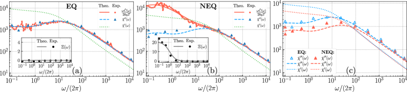
Figure 2: Actomyosin networks. In analogy to Fig. 1, here we compare our model predictions for $\omega\tilde{C}(\omega)/(2k_{\text{B}}T)$ and $\tilde{\chi}^{\prime\prime}(\omega)$ (solid and broken curves) with experimental actomyosin-network data from Ref. [13] in the (a) absence and (b) presence of ATP. The insets show the spectral function $\Xi(\omega)$ defined in Eq. (7). (c) Actomyosin networks exhibit a decrease of the real and imaginary response $\tilde{\chi}^{\prime}(\omega)$ and $\tilde{\chi}^{\prime\prime}(\omega)$ in NEQ.

By summing over the active particles and introducing collective variables $x(t)={\sum_{i}x_{i}(t)}/{n}$ and $f(t)={\sum_{i}f_{i}(t)}/{n}$, we obtain two coupled GLEs

$$M\ddot{X}(t)= -\gamma\int_{-\infty}^{t}{\mathrm{d}}t^{\prime}\,\mathcal{K}_{+}(t-t^{\prime})\dot{X}(t^{\prime})-(nk+K)X(t)$$

$$+nkx(t)+F(t),$$ (3a)

$$m\ddot{x}(t)= -\gamma_{\text{a}}\int_{-\infty}^{t}{\mathrm{d}}t^{\prime}\,\mathcal{K}_{+}(t-t^{\prime})\dot{x}(t^{\prime})-k(x(t)-X(t))$$

$$+f(t),$$ (3b)

for the tracer and the collective active-particle coordinate. The collective random noise has zero mean and strength $\langle f(t)f(t^{\prime})\rangle=k_{\text{B}}T_{\text{a}}\;\gamma_{\text{a}}\mathcal{K}_{+}(|t-t^{\prime}|)/n$.

By Fourier transforming, Eq.(3) can be solved for $\tilde{X}(\omega)=\int\!\mathrm{d}t\,X(t)\,{\text{e}}^{\dot{\iota}\omega t}$ to yield

$$\tilde{X}(\omega)=\frac{\tilde{F}_{\text{R}}(\omega)}{-M\omega^{2}+\dot{\iota}\omega\tilde{\mathcal{K}}_{\text{tot}}(\omega)+K},$$ (4)

with the effective friction kernel and the effective noise given by

$$\tilde{\mathcal{K}}_{\text{tot}}(\omega)=\bigg{[}\gamma\tilde{\mathcal{K}}_{+}(\omega)+\frac{nk\gamma_{\text{a}}\tilde{\mathcal{K}}_{+}(\omega)}{\dot{\iota}\omega\gamma_{\text{a}}\tilde{\mathcal{K}}_{+}(\omega)+k}\bigg{]},$$ (5)

$$\tilde{F}_{\text{R}}(\omega)=\frac{nk\tilde{f}(\omega)}{\dot{\iota}\omega\gamma_{\text{a}}\tilde{\mathcal{K}}_{+}(\omega)+k}+\tilde{F}(\omega).$$ (6)

From Eq. (4) we can directly calculate the positional autocorrelation function, $\tilde{C}(\omega)=\int\!\mathrm{d}t\,\langle X(0)X(t)\rangle\,{\text{e}}^{\dot{\iota}\omega t}$. From the linear-response relation $X(t)=\int_{0}^{\infty}\mathrm{d}t^{\prime}\chi(t-t^{\prime})F_{\text{R}}(t^{\prime})$, the imaginary part of the response function $\tilde{\tilde{\chi}}^{\prime\prime}(\omega)$ follows, see Supplemental Material [46] for explicit derivations. The FDT violation can be quantified by the spectral function [37]

$$\Xi(\omega)=\frac{\omega\tilde{C}(\omega)/(2k_{\text{B}}T)}{\tilde{\chi}^{\prime\prime}(\omega)}-1=\frac{\tilde{C}_{F}(\omega)/(2k_{\text{B}}T)}{\tilde{\mathcal{K}}^{\prime}_{\text{tot}}(\omega)}-1,$$ (7)

where $\tilde{C}_{F}(\omega)=\int\!\mathrm{d}t\,\langle F_{\text{R}}(0)F_{\text{R}}(t)\rangle\,{\text{e}}^{\dot{\iota}\omega t}$ is the spectral noise autocorrelation and $\tilde{\mathcal{K}}^{\prime}_{\text{tot}}(\omega)$ the real part of the Fourier-transformed memory kernel [46]. For an equilibrium system characterized by $\alpha=0$, i.e. when the active and tracer particles have the same temperature, the FDT is recovered [47] and $\Xi(\omega)=0$. Assuming overdamped motion with $M\rightarrow 0$ and $m\rightarrow 0$, we obtain explicitly

$$\tilde{\chi}^{\prime\prime}(\omega)= \,\omega^{\kappa}\sin\left(\frac{\kappa\pi}{2}\right)\bigg{[}(\gamma+\hat{\gamma}_{\text{a}})\hat{k}^{2}+2\gamma\hat{\gamma}_{\text{a}}\hat{k}\cos\left(\frac{\kappa\pi}{2}\right)\omega^{\kappa}+\gamma\hat{\gamma}_{\text{a}}^{2}\omega^{2\kappa}\bigg{]}\bigg{\{}\hat{k}^{2}K^{2}+\gamma^{2}\hat{\gamma}_{\text{a}}^{2}\omega^{4\kappa}$$

$$+\big{[}2\gamma\hat{\gamma}_{\text{a}}\hat{k}K\cos(\kappa\pi)+\left(\hat{\gamma}_{\text{a}}(\hat{k}+K)+\gamma\hat{k}\right)^{2}\big{]}\omega^{2\kappa}+2\cos\left(\frac{\kappa\pi}{2}\right)\big{[}\hat{\gamma}_{\text{a}}(\hat{k}+K)+\gamma\hat{k}\big{]}\big{[}\hat{k}K+\gamma\hat{\gamma}_{\text{a}}\omega^{2\kappa}\big{]}\omega^{\kappa}\bigg{\}}^{-1},$$

$$\tilde{C}(\omega)= \,2k_{\text{B}}T\omega^{\kappa-1}\sin\left(\frac{\kappa\pi}{2}\right)\bigg{[}(\gamma+\hat{\gamma}_{\text{a}}(1+\alpha))\hat{k}^{2}+2\gamma\hat{\gamma}_{\text{a}}\hat{k}\cos\left(\frac{\kappa\pi}{2}\right)\omega^{\kappa}+\gamma\hat{\gamma}_{\text{a}}^{2}\omega^{2\kappa}\bigg{]}\bigg{\{}\hat{k}^{2}K^{2}+\gamma^{2}\hat{\gamma}_{\text{a}}^{2}\omega^{4\kappa}$$

$$+\big{[}2\gamma\hat{\gamma}_{\text{a}}\hat{k}K\cos(\kappa\pi)+\left(\hat{\gamma}_{\text{a}}(\hat{k}+K)+\gamma\hat{k}\right){}^{2}\big{]}\omega^{2\kappa}+2\cos\left(\frac{\kappa\pi}{2}\right)\big{[}\hat{\gamma}_{\text{a}}(\hat{k}+K)+\gamma\hat{k}\big{]}\big{[}\hat{k}K+\gamma\hat{\gamma}_{\text{a}}\omega^{2\kappa}\big{]}\omega^{\kappa}\bigg{\}}^{-1},$$

$$\Xi(\omega)=\frac{\hat{\gamma}_{\text{a}}\hat{k}^{2}\alpha}{(\gamma+\hat{\gamma}_{\text{a}})\hat{k}^{2}+2\gamma\hat{\gamma}_{\text{a}}\hat{k}\cos\left(\frac{\kappa\pi}{2}\right)\omega^{\kappa}+\gamma\hat{\gamma}_{\text{a}}^{2}\omega^{2\kappa}},$$ (10)

where the active-particle number $n$ only appears implicitly via $\hat{\gamma}_{\text{a}}=n\gamma_{\text{a}}$ and $\hat{k}=nk$, so we are left with six parameters, the non-equilibrium parameter $\alpha$, the powerlaw exponent $\kappa$, the tracer and active-particle drag coefficients $\gamma$ and $\hat{\gamma}_{\text{a}}$, the tracer confinement strength $K$ and the tracer-active-particle elastic coupling strength $\hat{k}$. We consider two recent microrheology experiments on RBC flickering [20] and cross-linked F-actin networks with myosin II molecular motors [13], both reporting FDT violation by independently measuring $\tilde{\chi}^{\prime\prime}(\omega)$ and $\tilde{C}(\omega)$. For both experimental systems, it was shown that the FDT remains valid at short times or high frequencies, while strong FDT deviations are observed at long times or low frequencies. We digitize the experimental data reported for $\tilde{\chi}^{\prime\prime}(\omega)$ and $\omega\tilde{C}(\omega)/(2k_{\text{B}}T)$ and first fit their high-frequency limits, which from Eq. (Non-Markovian modeling of non-equilibrium fluctuations and dissipation in active viscoelastic biomatter) and Eq. (Non-Markovian modeling of non-equilibrium fluctuations and dissipation in active viscoelastic biomatter) are predicted as $\tilde{\chi}^{\prime\prime}(\omega)\simeq\sin(\frac{\kappa\pi}{2})/(\gamma\,\omega^{\kappa})$ and $\omega\tilde{C}(\omega)/(2k_{\text{B}}T)\simeq\sin(\frac{\kappa\pi}{2})/(\gamma\,\omega^{\kappa})$ and obtain $\kappa$ and $\gamma$ for each data set. Then, we simultaneous fit Eqs. (Non-Markovian modeling of non-equilibrium fluctuations and dissipation in active viscoelastic biomatter)-(Non-Markovian modeling of non-equilibrium fluctuations and dissipation in active viscoelastic biomatter) in the entire frequency range to find the remaining four parameters, the fitting parameters are shown in Table 1, see Supplemental Material [46] for details on the fitting procedure and a discussion of the uniqueness of the resulting fit parameters.

We start with the discussion of the RBC data, where the flickering dynamics of the RBC membrane was investigated by tracking the motion of a tracer bead attached to the RBC membrane in an equatorial position. In the experiments both the in vivo (NEQ) and the ATP-depleted scenarios were considered [20], we denote the latter scenario as EQ although a finite residual ATP concentration is present, the consequences of which will be discussed further below. In Fig. 1a,b we find excellent agreement between the experimental data and the fits for $\tilde{\chi}^{\prime\prime}(\omega)$ and $\omega\tilde{C}(\omega)/(2k_{\text{B}}T)$ for both EQ and NEQ scenarios in the entire frequency range. We also show the real (storage) part of the response function $\tilde{\chi}^{\prime}(\omega)$ from our model as dotted lines in Fig. 1a,b,c, see Supplemental Material [46] for the explicit expression. In the EQ case $\tilde{\chi}^{\prime\prime}(\omega)$ and $\omega\tilde{C}(\omega)/(2k_{\text{B}}T)$ agree rather nicely and display a weak minimum around $\omega/(2\pi)=2$ s^-1, that is caused by the competing elastic and friction effects, see Supplemental Material [46] for an asymptotic analysis of the response for low and high frequencies. In contrast, in the NEQ case the scaled autocorrelation $\omega\tilde{C}(\omega)/(2k_{\text{B}}T)$ is much larger than the response function $\tilde{\chi}^{\prime\prime}(\omega)$, indicating strong FDT violation. The spectral function $\Xi(\omega)$ in the insets illustrates that FDT violation occurs predominantly at low frequencies. The comparison in Fig. 1c demonstrates that both real and imaginary parts of the response function increase for NEQ at low frequencies, i.e. the effective stiffness of the network decreases at NEQ (see Supplemental Material [46] for a discussion of the low-/high-frequency asymptotic response). The viscoelastic power-law exponents for NEQ and EQ RBC experiments turn out to be $\kappa=0.936$ and $\kappa=0.926$ (see Table 1), respectively, which fall in the previously reported range $\kappa=0.92-1.07$ for fresh and aged RBCs [43]. The fitted trap stiffness in the NEQ case, $K=1.66\pm 0.03$ pN/$\mu$m, agrees with the experimentally reported value $1.56\pm 0.3$ pN/$\mu$m [20], for the EQ scenario our fitted stiffness is substantially higher, which presumably reflects added stiffness due to the viscoelastic EQ environment of the tracer particle. Our fit results for the coupling strength between tracer and active particles $\hat{k}$ is of the same order of $K$. Also, the fitted values of the tracer bead friction coefficient $\gamma$ in Table 1 are close to the experimentally reported value for the bare tracer bead $\gamma=0.085$ pN s/$\mu$m[20] for both NEQ and EQ scenarios, the fit results for the active-particle friction coefficients $\hat{\gamma}_{\text{a}}$ are of the same order. The good agreement between the fit parameters and the known experimental parameters shows that the model and the fitting procedure are robust. The non-equilibrium parameter in the NEQ case turns out to be $\alpha=36$ and thus indicates strong departures from EQ behavior. In the EQ case we obtain a non-zero value $\alpha\simeq 0.985$, which indicates weak NEQ due to incomplete ATP depletion in the experiment, as reflected by weak deviation between $\tilde{\chi}^{\prime\prime}(\omega)$ and $\omega\tilde{C}(\omega)/(2k_{\text{B}}T)$ in Fig. 1a.

Mizuno et al. [13] have studied the in vitro mechanics of active cross-linked actomyosin networks in the presence and absence of ATP, again referred to as NEQ and EQ cases.

The myosin-II motor proteins perform stepwise motion along the actin filaments in the presence of ATP, which causes sliding motion between two filaments connected by motors and thereby produces contractile active forces in the network. As shown in Fig. 2a, b, we again find excellent agreement between the experimental data and our fits for $\tilde{\chi}^{\prime\prime}(\omega)$ and $\omega\tilde{C}(\omega)/(2k_{\text{B}}T)$ for both the EQ and the NEQ scenarios in the entire frequency range. In the EQ case $\tilde{\chi}^{\prime\prime}(\omega)$ and $\omega\tilde{C}(\omega)/(2k_{\text{B}}T)$ are practically identical and show (similar to RBC) two weak maxima that are well produced by the model, see Supplemental Material [46] for an asymptotic analysis. In the NEQ case the scaled autocorrelation $\omega\tilde{C}(\omega)/(2k_{\text{B}}T)$ is much larger than the response function $\tilde{\chi}^{\prime\prime}(\omega)$, indicating strong FDT violation with a magnitude rather similar to the RBC case. For the EQ case the value $\alpha=-0.035$ indicates equilibrium in the absence of ATP. In both EQ and NEQ cases the fitted power-law exponent in Table 1 is in excellent agreement with $\kappa=3/4$ predicted by theory [48, 1, 10] and experiments [13]. The comparison in Fig. 1c demonstrates that both real and imaginary parts of the response function are at low frequencies for the NEQ case smaller than for the EQ case, i.e. the effective stiffness of the network increases in the NEQ case, in contrast to the RBC case. This behavior is primarily caused by the elastic model parameters: we see that $K$, which describes the stiffness of the tracer bead confinement, and $\hat{k}$, which describes the coupling strength between the tracer and the active particles, increase for actomyosin networks when going from the EQ to the NEQ scenario, whereas the opposite trend is observed for the RBC flickering data, see Table 1.

In summary, we introduce a simple model for viscoelastic active biomatter that incorporates the elastic coupling between a tracer bead and active particles and the medium viscoelasticity through a memory kernel and yields closed-form analytical predictions for the autocorrelation and response function of the tracer bead. These predictions are in excellent agreement with experimental data for RBCs and actomyosin networks and in particular allow to quantify the departure from EQ by the NEQ parameter $\alpha$, which corresponds to the effective temperature ratio of the reservoirs coupled to the active particles and the tracer bead in our model. We find $\alpha\approx 23$ and 36 in the presence of ATP and $\alpha\approx 0$ and 1 in the absence of ATP in the two experimental systems we considered, clearly signaling the strong NEQ character induced by ATP. Note that the effective temperature of the active particles does not correspond to the actual physical temperature, but rather characterizes the strength of the stochastic force the motor proteins produce and the power they dissipate. Our model has a wide range of applicability for active biomaterials and experimental setups and with suitable modifications can for example predict cross-correlations in two-particle microrheology experiments [49].

We acknowledge Hélène Berthoumieux for useful comments on manuscript. A.A. and R.R.N. acknowledge funding from the European Research Council (ERC) under the European Union’s Horizon 2020 Research and Innovation Program under Grant Agreement No. 835117. A.A. acknowledges the hospitality by the Institute for Research in Fundamental Sciences (IPM), Tehran, during the initial stages of this work.

References

- Schnurr et al. [1997] B. Schnurr, F. Gittes, F. C. MacKintosh, and C. F. Schmidt, Macromolecules 30, 7781 (1997).
- Joanny and Prost [2009] J. Joanny and J. Prost, HFSP Journal 3, 94 (2009).
- Osada and Gong [1998] Y. Osada and J.-P. Gong, Advanced Materials 10, 827 (1998).
- Bershadsky and Vasiliev [2012] A. D. Bershadsky and J. M. Vasiliev, Cytoskeleton (Springer Science & Business Media, 2012).
- Elson [1988] E. L. Elson, Annual Review of Biophysics and Biophysical Chemistry 17, 397 (1988).
- Jülicher et al. [2007] F. Jülicher, K. Kruse, J. Prost, and J.-F. Joanny, Physics Reports 449, 3 (2007).
- Fletcher and Mullins [2010] D. A. Fletcher and R. D. Mullins, Nature 463, 485 (2010).
- Lieleg et al. [2010] O. Lieleg, M. M. Claessens, and A. R. Bausch, Soft Matter 6, 218 (2010).
- Pelletier et al. [2003] O. Pelletier, E. Pokidysheva, L. S. Hirst, N. Bouxsein, Y. Li, and C. R. Safinya, Phys. Rev. Lett. 91, 148102 (2003).
- Hiraiwa and Netz [2018] T. Hiraiwa and R. R. Netz, Europhysics Letters 123, 58002 (2018).
- Rayment et al. [1993] I. Rayment, H. Holden, M. Whittaker, C. Yohn, M. Lorenz, K. Holmes, and R. Milligan, Science 261, 58 (1993).
- Martin et al. [2009] A. C. Martin, M. Kaschube, and E. F. Wieschaus, Nature 457, 495 (2009).
- Mizuno et al. [2007] D. Mizuno, C. Tardin, C. F. Schmidt, and F. C. MacKintosh, Science 315, 370 (2007).
- Mills et al. [2004] J. Mills, L. Qie, M. Dao, C. Lim, and S. Suresh, MCB Mol. Cell. Biomech. 1, 169 (2004).
- Puig-de Morales-Marinkovic et al. [2007] M. Puig-de Morales-Marinkovic, K. T. Turner, J. P. Butler, J. J. Fredberg, and S. Suresh, American Journal of Physiology-Cell Physiology 293, C597 (2007).
- Tuvia et al. [1997] S. Tuvia, A. Almagor, A. Bitler, S. Levin, R. Korenstein, and S. Yedgar, Proceedings of the National Academy of Sciences 94, 5045 (1997).
- Faris et al. [2009] M. D. E. A. Faris, D. Lacoste, J. Pécréaux, J.-F. Joanny, J. Prost, and P. Bassereau, Physical Review Letters 102, 038102 (2009).
- Betz and Sykes [2012] T. Betz and C. Sykes, Soft Matter 8, 5317 (2012).
- Girard et al. [2005] P. Girard, J. Prost, and P. Bassereau, Physical Review Letters 94, 088102 (2005).
- Turlier et al. [2016] H. Turlier, D. A. Fedosov, B. Audoly, T. Auth, N. S. Gov, C. Sykes, J.-F. Joanny, G. Gompper, and T. Betz, Nat. Phys. 12, 513 (2016).
- Bernheim-Groswasser et al. [2018] A. Bernheim-Groswasser, N. S. Gov, S. A. Safran, and S. Tzlil, Adv. Mater. 30, 1707028 (2018).
- Rädler et al. [1995] J. O. Rädler, T. J. Feder, H. H. Strey, and E. Sackmann, Physical Review E 51, 4526 (1995).
- Manneville et al. [1999] J.-B. Manneville, P. Bassereau, D. Lévy, and J. Prost, Phys. Rev. Lett. 82, 4356 (1999).
- Mizuno et al. [2008] D. Mizuno, D. Head, F. MacKintosh, and C. Schmidt, Macromolecules 41, 7194 (2008).
- Betz et al. [2009] T. Betz, M. Lenz, J.-F. Joanny, and C. Sykes, Proc. Natl. Acad. Sci. U. S. A. 106, 15320 (2009).
- Park et al. [2010] Y. Park, C. A. Best, T. Auth, N. S. Gov, S. A. Safran, G. Popescu, S. Suresh, and M. S. Feld, Proceedings of the National Academy of Sciences 107, 1289 (2010).
- Mauri and Leporini [2006] R. Mauri and D. Leporini, Europhysics Letters (EPL) 76, 1022 (2006).
- Berthier and Barrat [2002] L. Berthier and J.-L. Barrat, The Journal of Chemical Physics 116, 6228 (2002).
- Szamel [2014] G. Szamel, Phys. Rev. E 90, 012111 (2014).
- Grigera and Israeloff [1999] T. S. Grigera and N. E. Israeloff, Phys. Rev. Lett. 83, 5038 (1999).
- Fodor et al. [2016] E. Fodor, C. Nardini, M. E. Cates, J. Tailleur, P. Visco, and F. van Wijland, Phys. Rev. Lett. 117, 038103 (2016).
- Ben-Isaac et al. [2011] E. Ben-Isaac, Y. Park, G. Popescu, F. L. H. Brown, N. S. Gov, and Y. Shokef, Phys. Rev. Lett. 106, 238103 (2011).
- Gov et al. [2003] N. Gov, A. G. Zilman, and S. Safran, Phys. Rev. Lett. 90, 228101 (2003).
- Rodríguez-García et al. [2015] R. Rodríguez-García, I. López-Montero, M. Mell, G. Egea, N. S. Gov, and F. Monroy, Biophys. J. 108, 2794 (2015).
- Gov and Safran [2005] N. S. Gov and S. A. Safran, Biophysical Journal 88, 1859 (2005).
- Lin et al. [2006] L. C.-L. Lin, N. Gov, and F. L. H. Brown, The Journal of Chemical Physics 124, 074903 (2006).
- Netz [2018] R. R. Netz, J. Chem. Phys. 148, 185101 (2018).
- Schwarz and Safran [2013] U. S. Schwarz and S. A. Safran, Rev. Mod. Phys. 85, 1327 (2013).
- Goychuk [2012] I. Goychuk, Advances in Chemical Physics 150, 187 (2012).
- Mainardi [1997] F. Mainardi, in Fractals and fractional calculus in continuum mechanics (Springer, 1997) p. 291.
- Fabry et al. [2001] B. Fabry, G. N. Maksym, J. P. Butler, M. Glogauer, D. Navajas, and J. J. Fredberg, Phys. Rev. Lett. 87, 148102 (2001).
- Bursac et al. [2007] P. Bursac, B. Fabry, X. Trepat, G. Lenormand, J. P. Butler, N. Wang, J. J. Fredberg, and S. S. An, Biochemical and Biophysical Research Communications 355, 324 (2007).
- Costa et al. [2008] M. Costa, I. Ghiran, C.-K. Peng, A. Nicholson-Weller, and A. L. Goldberger, Phys. Rev. E 78, 020901 (2008).
- Kappler et al. [2019] J. Kappler, F. Noé, and R. R. Netz, Phys. Rev. Lett. 122, 067801 (2019).
- Taloni et al. [2010] A. Taloni, A. Chechkin, and J. Klafter, Phys. Rev. Lett. 104, 160602 (2010).
- [46] See Supplemental Material at [URL will be inserted by publisher] for derivations of all equations in the main text and details of the method used to fit the model predictions to the experimental data. We also provide results for alternative viscoelastic models such as the Maxwell and the Kelvin-Voigt model.
- Kubo et al. [2012] R. Kubo, M. Toda, and N. Hashitsume, Statistical physics II: nonequilibrium statistical mechanics, Vol. 31 (Springer Science & Business Media, 2012).
- Morse [1998] D. C. Morse, Phys. Rev. E 58, R1237 (1998).
- Mizuno et al. [2009] D. Mizuno, R. Bacabac, C. Tardin, D. Head, and C. F. Schmidt, Physical Review Letters 102, 1 (2009).