Quasi-normal modes of rotating black holes in Einstein-dilaton Gauss-Bonnet gravity: the second order in rotation

Abstract

One of the most promising strategies to test gravity in the strong-field, large curvature regime is gravitational spectroscopy: the measurement of black hole quasi-normal modes from the ringdown signal emitted in the aftermath of a compact binary coalescence, searching for deviations from the predictions of general relativity. This strategy is only effective if we know how quasi-normal modes of black holes are affected by modifications of general relativity; and if we know this for rotating black holes, since binary coalescences typically lead to black holes with spins $J/M^{2}\sim 0.7$. In this article, we compute for the first time the gravitational quasi-normal modes of rotating black holes up to second order in the spin in a modified gravity theory. We consider Einstein-dilaton Gauss-Bonnet gravity, one of the simplest theories which modifies the large-curvature regime of gravity and which can be tested with black hole observations. To enhance the domain of validity of the spin expansion, we perform a Pad éé resummation of the quasi-normal modes. We find that when the second order in spin is not included, the effect of gravity modifications may be seriously underestimated. A comparison with the general relativistic case suggests that this approach should be accurate up to spins $\sim 0.7$; therefore, our results can be used in the data analysis of ringdown signals.

I Introduction

In the last century, a plethora of observations confirmed that the gravitational interaction is well described by general relativity (GR) [1]. However, before 2015 – when the first gravitational wave (GW) signal was detected [2] – these tests were mostly limited to the weak-field regime of gravity. In recent years, the observations of the Advanced LIGO/Virgo detectors started to explore strong gravitational fields and large spacetime curvature, and have excluded large deviations of GR in this regime [3]. The next generation of GW detectors, like the ground-based Einstein Telescope [4], will be sensitive enough to detect even tiny GR deviations in the strong-field, large curvature regime of gravity.

One of the most promising strategies to find such deviations is the analysis of the ringdown signal emitted in the aftermath of a binary black hole (BH) coalescence. In this stage, the waveform is a superposition of damped oscillations, the quasi-normal modes (QNMs) of the final BH [5, 6, 7]. The QNM frequencies and damping times carry the imprint of the underlying theory of gravity; once measured from the GW signal, they can be compared with the predictions of GR, or - if a deviation is observed - with the predictions of a possible modified theory of gravity. With a more refined analysis, it is possible to improve the accuracy by stacking multiple observations [8, 9, 10].

This approach, which has been called “gravitational spectroscopy” [11, 12, 13] (see also [14] and references therein), requires the knowledge of the QNMs of BHs in modified gravity theories. The frequencies and damping times of BH QNMs have been computed for a certain number of such theories, for static, non-rotating BHs [15, 16, 17, 18, 19, 20, 21, 22] or for slowly rotating BHs at first order in the spin [23, 24, 25, 26].

However, since BH remnants of compact binary coalescences have typical spins – for comparable-mass binaries – of the order of $\bar{a}=J/M^{2}\sim 0.7$ (where $M,J$ are the mass and angular momentum of the BH, respectively), the knowledge of BH QNMs to $O(\bar{a})$ is inadequate to perform gravitational spectroscopy. Indeed, an analysis of the QNMs in GR suggests that the slowly rotating approximation at ${\cal O}(\bar{a})$ gives the QNM frequencies with an accuracy of $1\%$ for $\bar{a}\lesssim 0.2$ only (see Fig. 1 below). This article, to our knowledge, is the first computation of the QNMs of a slowly rotating BH to second order in the spin in a modified gravity theory. We shall argue that, with an appropriate resummation of the spin expansion, this computation is expected to be accurate for spins as large as $\bar{a}\sim 0.7$.

We shall consider Einstein-dilaton Gauss-Bonnet (EdGB) gravity, one of the simplest theories which modifies the strong-field, large-curvature regime of gravity, and which can be tested with BH observations (see [30] and references therein). In EdGB gravity the gravitational sector contains, besides the metric tensor, a scalar field (i.e., it is a scalar-tensor theory), which is coupled with the spacetime curvature through the Gauss-Bonnet term $\mathcal{R}^{2}_{\rm GB}=R_{\mu\nu\rho\sigma}R^{\mu\nu\rho\sigma}-4R_{\mu\nu}R^{\mu\nu}+R^{2}$, where $R_{\mu\nu\alpha\beta}$, $R_{\mu\nu}$, $R$ are the Riemann tensor, the Ricci tensor and the Ricci scalar, respectively. The action is [31, 32]:

$$S =\int d^{4}x\frac{\sqrt{-g}}{16\pi}\left(R-\frac{1}{2}\partial_{\mu}\phi\partial^{\mu}\phi+V(\phi)+\frac{\alpha_{\rm GB}}{4}e^{\phi}\mathcal{R}^{2}_{\rm GB}\right)$$

$$+S_{\rm m}$$ (1)

where $S_{\rm m}$ is the matter Lagrangian, which we do not consider in this paper since we are interested in BH spacetimes. We also neglect, for simplicity, the scalar field potential $V(\phi)$.

EdGB gravity naturally arises in low-energy truncations of string theories; it belongs to the class of Horndeski gravity [33, 34], i.e. the scalar-tensor theories with second-order-in-time field equations (which are thus free from the Ostrogradsky instability). At variance with several other scalar-tensor theories, EdGB gravity does not satisfy the no-hair theorems: stationary BHs have a non-trivial scalar field profile, and are not described by the Kerr metric.

As discussed in Sec. II, a static BH with mass $M$ can exist in EdGB gravity only if $\alpha_{\rm GB}/M^{2}\lesssim 0.69$; a similar bound applies for stationary, rotating BHs. Therefore, the existence of the lightest BH observed, J1655-40, with mass $M\simeq 5.4\,M_{\odot}$ implies $\sqrt{\alpha_{\rm GB}}<6.6$ Km. Current observations of binary BH coalescences by LIGO and Virgo lead to a comparable constraint, $\sqrt{\alpha_{\rm GB}}<9.1$ Km [35].

QNMs of BHs in EdGB gravity have been computed in [19] for non-rotating BHs, and in [23] (hereafter, Paper I) for rotating BHs at first order in the spin. In this article we shall compute the QNMs of stationary, rotating BHs in EdGB gravity, by performing a slow-rotation expansion, as in [37, 38, 39], to second order in the spin $\bar{a}$.

We shall use geometric units, $G=c=1$. In Section II we describe stationary BHs in EdGB gravity. In Section III we discuss perturbations of the stationary BH background, up to second order in $\bar{a}$. In Section IV we discuss the results of our computations, and in Section V we draw our conclusions. In the Appendix we give further details on the perturbation equations to second order in the spin.

II Stationary black holes in Einstein-dilaton Gauss-Bonnet gravity

The field equations obtained from (1) (with $V(\phi)=S_{m}=0$) are

$$\frac{1}{\sqrt{-g}}\partial_{\mu}(\sqrt{-g}g^{\mu\nu}\partial_{\nu}\phi)=\frac{\alpha_{\rm GB}}{4}e^{\phi}\mathcal{R}^{2}_{GB}$$ (2)

$$G_{\mu\nu}=\frac{1}{2}\partial_{\mu}\phi\partial_{\nu}\phi-\frac{1}{4}g_{\mu\nu}(\partial_{\rho}\phi)(\partial^{\rho}\phi)-\alpha_{\rm GB}\mathcal{K}_{\mu\nu}$$ (3)

where $G_{\mu\nu}$ is the Einstein tensor,

$$\mathcal{K}_{\mu\nu}=\frac{1}{8}(g_{\mu\rho}g_{\nu\sigma}+g_{\mu\sigma}g_{\nu\rho})\epsilon^{\delta\sigma\gamma\alpha}\nabla_{\beta}\left({\tilde{R}^{\rho\beta}}_{~{}~{}\gamma\alpha}e^{\phi}\partial_{\delta}\phi\right)\,,$$ (4)

$\epsilon^{\mu\nu\delta\gamma}$ is the Levi-Civita tensor, and ${\tilde{R}^{\mu\nu}}_{~{}~{}\rho\sigma}=\epsilon^{\mu\nu\delta\gamma}R_{\delta\gamma\rho\sigma}$.

II.1 Non-rotating black holes

The solution of Eqs. (2), (3) describing a static, spherically symmetric BH has been derived in [32] (see also [40]). In this case, the spacetime metric can be written as:

$$ds^{2}=-A(r)dt^{2}+\frac{dr^{2}}{B(r)}+r^{2}d\Omega^{2}$$ (5)

where $d\Omega^{2}=d\theta^{2}+\sin^{2}\theta d\varphi^{2}$. The functions $A(r)$, $B(r)$ and $\phi(r)$ are found by numerical integration [32, 40]. By requiring asymptotic flatness and an asymptotically vanishing scalar field, one finds an unique solution, with an ADM mass $M$ and a scalar charge $D$ which appear in the asymptotic expansion of the metric and of the scalar field:

$$A =1-\frac{2M}{r}+O\left(\frac{1}{r^{3}}\right)$$

$$\phi =\frac{D}{r}+\frac{DM}{r^{2}}+O\left(\frac{1}{r^{3}}\right)\,.$$ (6)

The solution depends on $\alpha_{\rm GB}$ through the dimensionless coupling parameter

$$\zeta=\frac{\alpha_{\rm GB}}{M^{2}}\,,$$ (7)

which has to satisfy the condition

$$0\leq\zeta<\zeta_{\rm max}\simeq 0.691\,.$$ (8)

If $\zeta\geq\zeta_{\rm max}$, it is not possible to enforce regular boundary conditions on the horizon, and the BH becomes a naked singularity [41].

The scalar charge $D$ and the horizon radius $r_{\rm h}$ depend on the BH mass and of the coupling $\zeta$:

$$\frac{D}{M} =\frac{\zeta}{2}+\frac{73}{60}\zeta^{2}+O(\zeta^{3})$$

$$\frac{r_{\rm h}}{2M} =1-\frac{49}{1280}\,\zeta^{2}+O(\zeta^{3})\,.$$ (9)

For a given value of the coupling constant $\alpha_{\rm GB}$, there is a single static, spherically symmetric BH solution for each value of the mass satisfying $M\geq M_{\rm min}=\alpha_{\rm GB}\zeta^{-1/2}_{\rm max}$.

The field equations (2), (3) can also be solved perturbatively in the parameter $\zeta$ [42]. This leads to an analytic expression for the metric and the scalar field:

$$A(r) =1-\frac{2M}{r}+\sum_{j=2}^{N_{\zeta}}\zeta^{j}A^{(j)}(r)$$

$$B(r) =1-\frac{2M}{r}+\sum_{j=2}^{N_{\zeta}}\zeta^{j}B^{(j)}(r)$$

$$\phi(r) =\sum_{j=1}^{N_{\zeta}}\zeta^{j}\phi^{(j)}(r)$$ (10)

where $A^{(j)}(r)$, $B^{(j)}(r)$ and $\phi^{(j)}(r)$ can be written as expansions in powers of $1/r$.

II.2 Rotating black holes

In the case of stationary, rotating BHs, Eqs. (2), (4) have been solved numerically in Refs. [43, 44], with no assumptions on the rotation rate. They have also been solved analytically [40, 45] in terms of a perturbative expansion in the coupling parameter $\zeta$ and in the spin ${\bar{a}}$:

$$ds^{2} =-A(r)[1+2h(r,\theta)]dt^{2}+\frac{1}{B(r)}[1+2p(r,\theta)]dr^{2}$$

$$+r^{2}[1+2k(r,\theta)]\left[d\theta^{2}+\sin^{2}\theta(d\varphi-\varpi(r,\theta)dt)^{2}\right]$$ (11)

where $A(r)$, $B(r)$, $\phi(r)$ are given in Eqs. (10), while $\varpi(r,\theta)$, $h(r,\theta)$, $p(r,\theta)$ and the scalar field $\phi(r,\theta)$ are given as expansions in $\zeta$, $\bar{a}$ and in the Legendre polynomials $P_{l}(\theta)$. For instance, the scalar field expansion is:

$$\phi(r)=\sum_{j=1}^{N_{\zeta}}\,\,\sum_{n=0,2,4,...}^{N_{\bar{a}}}\,\,\sum_{l=0,2,4...}^{n}\zeta^{j}{\bar{a}}^{n}\phi_{l}^{(nj)}(r)P_{l}(\theta)\,,$$ (12)

where $N_{\zeta}$, $N_{a}$, $n$ are the truncation orders of the expansions in the coupling, in the spin and in the Legendre polynomials. The expansions of $\varpi(r,\theta)$, $h(r,\theta)$, $p(r,\theta)$ have the same structure. Note that for $\zeta=0$ (i.e., in GR) the metric (II.2) reduces to the Hartle-Thorne metric [37].

The explicit expression of this expansion is given in [45] and in the Mathematica notebook in the Supplemental Material [46]. Similarly, the horizon radius $r_{\rm h}$, the scalar charge $D$ and the maximum allowed coupling $\zeta_{\rm max}$ acquire corrections with respect to the non-rotating case, and can be expressed as expansions in $\zeta$ and ${\bar{a}}$.

In the following we shall study perturbations around the slowly rotating BH background given by the expansion (II.2), (12). We shall truncate the spin expansion at $N_{\bar{a}}=2$. As discussed in Sec. IV.1, an assessment of the slow-rotation expansion in GR, and an analysis of the truncation error at different orders in the coupling, suggest that in this way we should be able to compute the QNMs, for $\bar{a}\sim 0.4$, with truncation errors within $\sim 1\%$, and for $\bar{a}\sim 0.7$, with truncation errors within $\sim 5\%$. Moreover, we shall truncate the expansion in the coupling at $N_{\zeta}=6$; this should lead to errors within $\sim 1\%$ for coupling constant $\zeta\sim 0.4$ for the real part of the QNMs, and for $\zeta\sim 0.3$ for the imaginary part.

III Perturbations of Einstein-dilaton Gauss-Bonnet black holes

We consider a perturbed stationary, rotating BH. The spacetime metric and the scalar field are

$$g_{\mu\nu} =g^{(0)}_{\mu\nu}+h_{\mu\nu}^{\rm pol}+h_{\mu\nu}^{\rm ax}$$

$$\phi =\phi^{(0)}+\delta\phi$$ (13)

where $g^{(0)}_{\mu\nu}$, $\phi^{(0)}$ are given by Eqs. (II.2), (12). The metric perturbation is decomposed in components with polar and axial parities.

III.1 General structure of the equations

The perturbations of the metric tensor and of the scalar field are expanded in tensor spherical harmonics as:

$$\delta\phi(t,r,\theta,\varphi)=\frac{1}{r}\Phi^{lm}(r)Y^{lm}(\theta,\varphi)e^{-i\omega t}\,,$$ (14)

$$h^{\rm pol}_{\mu\nu}(t,r,\theta,\varphi)dx^{\mu}dx^{\nu}=$$

$$\left[A(r)H_{0}^{lm}(r)dt^{2}+2H_{1}^{lm}(r)dtdr+B^{-1}(r)H_{2}^{lm}(r)dr^{2}\right.$$

$$\left.+K^{lm}(r)(dr^{2}+\sin^{2}\theta d\varphi^{2})\right]Y^{lm}(\theta,\varphi)e^{-i\omega t}\,,$$ (15)

$$h^{\rm ax}_{\mu\nu}dx^{\mu}dx^{\nu}=2(h_{0}^{lm}(r)dt+h_{1}^{lm}(r)dr)$$

$$\times(S_{\theta}(\theta,\varphi)d\theta+S_{\varphi}(\theta,\varphi)d\varphi)e^{-i\omega t}$$ (16)

where we have chosen the Regge-Wheeler gauge [47, 48], and $(S^{lm}_{\theta},S^{lm}_{\varphi})=(-(\sin\theta)^{-1}Y^{lm}_{,\varphi},\sin\theta Y^{lm}_{,\theta})$. Replacing this expansion in Eqs. (2), (3) leads to a set of partial differential equations in $r$ and $\theta$ (see App. A). Due to the stationarity and axial symmetry of the background, the dependence on on $t$ and $\varphi$ factors out as $\sim e^{i(m\varphi-\omega t)}$, and the equations with different values of $m,\omega$ are decoupled.

Following e.g. [49] (see also [50] and Paper I), we can reduce the perturbation equations to a system of ordinary differential equations in $r$, up to second order in the spin. Since the background is not spherically symmetric, equations with different values of $l$ are coupled. Schematically, the general structure of the perturbation equations can be written as:

$$0= {\cal{P}}_{l\,m}+{\bar{a}}\,m\,\bar{\cal{P}}_{l\,m}+{\bar{a}}^{2}\hat{\cal{P}}_{l\,m}+\,m^{2}\,{\bar{a}}^{2}{\bar{\bar{\cal{P}}}}_{l\,m}$$

$$+{\bar{a}}\left(Q_{l\,m}\tilde{\cal{A}}_{l-1\,m}+Q_{l+1\,m}\tilde{\cal{A}}_{l+1\,m}\right)$$

$$+{\bar{a}}^{2}\left(Q_{l-1\,m}Q_{l\,m}\breve{\cal{P}}_{l-2\,m}+Q_{l+1\,m}Q_{l+2\,m}\breve{\cal{P}}_{l+2\,m}\right)$$

$$+m\,{\bar{a}}^{2}\left(Q_{l\,m}\check{\cal{A}}_{l-1\,m}+Q_{l+1\,m}\check{\cal{A}}_{l+1\,m}\right)$$ (17)

$$0= {\cal{A}}_{l\,m}+{\bar{a}}\,m\,\bar{\cal{A}}_{l\,m}+{\bar{a}}^{2}\hat{\cal{A}}_{lm}+\,m^{2}\,{\bar{a}}^{2}{\bar{\bar{\cal{A}}}}_{l\,m}$$

$$+{\bar{a}}\left(Q_{l\,m}\tilde{\cal{P}}_{l-1\,m}+Q_{l+1\,m}\tilde{\cal{P}}_{l+1\,m}\right)$$

$$+{\bar{a}}^{2}\left(Q_{l-1\,m}Q_{l\,m}\breve{\cal{A}}_{l-2\,m}+Q_{l+1\,m}Q_{l+2\,m}\breve{\cal{A}}_{l+2\,m}\right)$$

$$+m\,{\bar{a}}^{2}\left(Q_{l\,m}\check{\cal{P}}_{l-1\,m}+Q_{l+1\,m}\check{\cal{P}}_{l+1\,m}\right)$$ (18)

where $Q_{lm}$ are constant coefficients, and ${\cal P}_{lm}$, $\bar{\cal P}_{lm}$, $\hat{\cal P}_{lm}$, ${\bar{\bar{\cal{P}}}}_{l\,m}$, $\tilde{\cal{P}}_{l\,m}$, $\breve{\cal{P}}_{l\,m}$, $\check{\cal{P}}_{l\,m}$, (${\cal A}_{lm}$, $\bar{\cal A}_{lm}$, $\hat{\cal A}_{lm}$, ${\bar{\bar{\cal{A}}}}_{l\,m}$, $\tilde{\cal{A}}_{l\,m}$, $\breve{\cal{A}}_{l\,m}$, $\check{\cal{A}}_{l\,m}$) are combinations of the polar perturbation functions $H_{0}^{lm}$, $H_{1}^{lm}$, $H_{2}^{lm}$, $K^{lm}$, $\Phi^{lm}$ (of the axial perturbation functions $h_{0}^{lm}$, $h_{1}^{lm}$). We remark that the expressions ${\cal P}_{lm}$, etc. do not depend explicitly on the harmonic index $m$. For further details, see Appendix A and the Supplemental Material [46].

While at zero-th order in the spin the equations (${\cal P}_{lm}=0$, ${\cal A}_{lm}=0$) are decoupled, at first order in the spin polar perturbations with harmonic index $l$ are coupled to axial perturbations with harmonic indexes $l\pm 1$, and vice versa. Moreover, when $m\neq 0$ polar (axial) perturbations are coupled to perturbations having the same $l$ and the same parity (see the discussion in Paper I). At second order in the spin, perturbations with harmonic index $l$ are also coupled to perturbations with same parities and harmonic indexes $l\pm 2$, and (when $m\neq 0$) to perturbations with opposite parities and harmonic indexes $l\pm 1$.

III.2 Quasi-normal modes

The QNMs are the proper modes at which BHs (or compact stars) oscillate when excited by non-radial perturbations (see e.g. [5, 6, 7] and references therein). At variance with normal modes, the QNMs are damped oscillations, since they are associated to GW emission. Therefore the corresponding frequencies $\omega$ (see Eqs. (14)-(16)) are complex: $\omega=\omega_{R}+i\,\omega_{I}$, with $\omega_{I}<0$ being the inverse of the damping time of the oscillation.

To find the QNM frequencies, we solve the perturbation equations with Sommerfeld boundary conditions, i.e. outgoing waves at infinity and ingoing waves at the horizon. At the horizon and at infinity, the scalar ($\Phi^{lm}(r)$) and gravitational ($H^{lm}_{1}(r)/r$, $K^{lm}(r)$, etc.) perturbation functions behave as

$$A_{\rm in}^{lm}e^{-ik_{\rm H}r_{*}}+A_{\rm out}^{lm}e^{ik_{\rm H}r_{*}}~{}\,~{}~{}~{}(r\to r_{\rm h})$$

$$A_{\rm in}^{lm}e^{-i\omega r_{*}}+A_{\rm out}^{lm}e^{i\omega r_{*}}~{}~{}~{}~{}~{}~{}~{}(r\to\infty)\,,$$ (19)

where $r_{*}$ is a properly defined tortoise coordinate for the background spacetime $g^{(0)}_{\mu\nu}$ (see below), and

$$k_{\rm H}=\omega-m\Omega_{\rm H}~{}~{}~{}{\rm with}~{}~{}~{}\Omega_{\rm H}=-\lim_{r\to r_{\rm h}}\frac{g_{t\varphi}}{g_{\varphi\varphi}}\,.$$ (20)

At the horizon and at infinity the couplings (between scalar and gravitational perturbations, and between perturbations with different values of $l$) are subleading, and the perturbation equations can be written as two second-order differential equations with the structure (with $Z^{lm}$ being either $\Phi^{lm}$ or $K^{lm}$)

$$Z^{lm}_{,r_{*}r_{*}}+k_{H}^{2}Z^{lm} =O(r-r_{\rm h})~{}~{}~{}~{}~{}(r\to r_{\rm h})$$

$$Z^{lm}_{,r_{*}r_{*}}+\omega^{2}Z^{lm} =O\left(\frac{1}{r^{2}}\right)~{}~{}~{}~{}~{}(r\to\infty)\,,$$ (21)

with boundary conditions

$$Z^{lm} \sim e^{-ik_{\rm H}r_{*}}~{}\,~{}~{}~{}{\rm at}~{}~{}(r\to r_{\rm h})$$

$$Z^{lm} \sim e^{\,i\omega r_{*}}~{}~{}~{}~{}~{}~{}~{}{\rm at}~{}~{}(r\to\infty)\,.$$ (22)

The tortoise coordinate $r_{*}(r)$ maps the region outside the BH horizon $r\in[r_{\rm h},\infty]$ into $r_{*}\in[-\infty,+\infty]$; the function

$$\frac{dr}{dr_{*}}=F(r)$$ (23)

behaves as $F(r)\sim r-r_{\rm h}$ for $r\to r_{\rm h}$, and $F(r)\to 1$ for $r\to\infty$. The explicit expression of $F(r)$ can be found by requiring that the perturbation equations reduce, at the horizon and at infinity, to Eq. (21).

Actually, for rotating BHs in EdGB gravity there are different possible functions $F(r)$ satisfying this requirement. In Paper I we have shown that by imposing a stronger requirement, i.e. that besides Eq. (21),

$$Z^{lm}_{,r_{*}r_{*}}+\omega^{2}Z^{lm}=\frac{l(l+1)}{r^{2}}Z^{lm}+O\left(\frac{1}{r^{3}}\right)$$ (24)

for $r\to\infty$, the function $F(r)$ is uniquely determined. To $O(\zeta^{2})$, it is

$$F(r)= \left(1-\frac{r_{\rm h}}{r}\right)\left\{1-{\bar{a}}^{2}\frac{r_{\rm h}(r^{2}+rr_{\rm h}+r_{\rm h}^{2})}{8r^{3}}\right.$$

$$\left.-\zeta^{2}\left[\frac{r_{\rm h}}{3840r^{4}}(147r^{3}+117r^{2}r_{\rm h}-526rr_{\rm h}^{2}+263r_{\rm h}^{3})\right.\right.$$

$$\left.\left.+{\bar{a}}^{2}\frac{r_{\rm h}}{30720r^{3}}(375r^{2}+435rr_{\rm h}+343r_{\rm h}^{2})\right]\right\}$$

$$+O(\zeta^{3})+O({\bar{a}}^{3})\,.$$ (25)

The explicit expression of $F(r)$ to $O(\zeta^{6})$ is given in the Supplemental Material [46]. We have verified that with a different definition of the tortoise coordinate – satisfying the condition (21) but not the stronger condition (24) – the values of the QNMs are the same within the numerical error.

We remark that both the equations (17), (18) and the boundary conditions for QNMs (22) are invariant for the transformation in $(\bar{a},m)\to(-\bar{a},-m)$ (note that $\Omega_{\rm H}\propto\bar{a}$), as long as axial perturbations change sign and polar perturbations remain the same. Therefore, the solution and the quasi-normal modes frequencies are invariant for this transformation as well. This implies that the $O(\bar{a})$ corrections in the spin are odd in $m$, while the second-order corrections are even (see e.g. [51] and Paper I). Since the equations are quadratic at most in $m$, we shall make the following ansatz for the QNM frequencies

$$\omega=\omega_{0}+{\bar{a}}\,m\omega_{1}+{\bar{a}}^{2}\,\left(\omega_{2a}+m^{2}\omega_{2b}\right)+O({\bar{a}}^{3})\,,$$ (26)

where $\omega_{r}$ ($r=0,1,2a,2b$) do not depend on $m$. This will be confirmed by the actual QNM computation.

III.3 Perturbation equations

We shall here discuss the derivation and the numerical implementation of the perturbation equations to second order in the spin. For the derivation in the non-rotating case and to first order in rotation, we refer the reader to [19] and to Paper I, respectively.

We decompose the metric and scalar field perturbations in terms of the perturbation functions of polar parity $\{H_{0}^{lm}(r),H_{1}^{lm}(r),H_{2}^{lm}(t,r),K^{lm}(r),\Phi^{lm}(r)\}$ and of axial parity $\{h_{0}^{lm}(r),h_{1}^{lm}(r)\}$ as in Eqs. (14)-(16). The field equations (2), (3), linearized in the perturbations and to second order in the spin, yield a system of ordinary differential equations, with the general structure (17), (18). We remark that the equations couple perturbations with different parities, and with different values of the harmonic index $l$.

As discussed in [52, 51, 38], the couplings of the perturbations with index $l$ to those with index $l\pm 1$ can be neglected in the computation of the QNM spectrum to first order in the spin. Similarly, as we are going to show, we can neglect the couplings between perturbations with index $l$ and with index $l\pm 2$ in the computation of the QNMs to second order in the spin.

Let us consider the expansion in the spin of the perturbation functions with polar parities $Z_{\rm pol}^{lm}$ ($=H_{0}^{lm}$, $H_{1}^{lm}$, …) and with axial parities $Z_{\rm ax}^{lm}$ ($=h_{0}^{lm}$, $h_{1}^{lm}$):

$$Z_{\rm pol/ax}^{lm}=Z_{\rm pol/ax}^{lm\,(0)}+\bar{a}\,Z_{\rm pol/ax}^{lm\,(1)}+\bar{a}^{2}\,Z_{\rm pol/ax}^{lm\,(2)}\,.$$ (27)

Since perturbations with index $l\pm 1$ are always multiplied by $\bar{a}$ in the equations (17), (18), their second-order term in the expansion (27) does not contribute to the equations; moreover, when they are multiplied by ${\bar{a}}^{2}$, their first-order terms does not contribute as well. Similarly, perturbations with index $l\pm 2$ contribute to the equations (17), (18) with their $0$-order part in the expansion (27) only.

Let us now assume that a source only excites a polar perturbation with a given harmonic index $l$. The rotation-induced couplings in the field equations induce perturbations with axial parity and with harmonic index $l^{\prime}\neq l$, but they vanish in the non-rotating limit: $Z_{\rm ax}^{lm\,(0)}=Z_{\rm pol}^{l^{\prime}m\,(0)}=0$. Axial parity perturbations with index $l\pm 1$ are excited through the rotation-induced couplings at first order in the spin, and are $Z_{\rm ax}^{l\pm 1m}=O(\bar{a})$; similarly, polar parity perturbations with index $l\pm 2$ are excited through the rotation-induced couplings at second order in the spin, and are $Z_{\rm pol}^{l\pm 2m}=O({\bar{a}}^{2})$. Therefore, neglecting $O({\bar{a}}^{3})$ terms, Eqs. (17), (18) reduce to

$${\cal{P}}_{l\,m}+{\bar{a}}\,m\,\bar{\cal{P}}_{l\,m}+{\bar{a}}^{2}\hat{\cal{P}}_{l\,m}+\,m^{2}\,{\bar{a}}^{2}{\bar{\bar{\cal{P}}}}_{l\,m}$$

$$+{\bar{a}}\left(Q_{l\,m}\tilde{\cal{A}}_{l-1\,m}+Q_{l+1\,m}\tilde{\cal{A}}_{l+1\,m}\right)=0$$

$${\cal{A}}_{l+1\,m}+{\bar{a}}\,m\,\bar{\cal{A}}_{l+1\,m}+{\bar{a}}\,Q_{l+1\,m}\tilde{\cal{P}}_{l\,m}$$

$$+m\,{\bar{a}}^{2}\,Q_{l+1\,m}\check{\cal{P}}_{l\,m}=0$$

$${\cal{A}}_{l-1\,m}+{\bar{a}}\,m\,\bar{\cal{A}}_{l-1\,m}+{\bar{a}}\,Q_{l\,m}\tilde{\cal{P}}_{l\,m}$$

$$+m\,{\bar{a}}^{2}\,Q_{l\,m}\check{\cal{P}}_{l\,m}=0\,.$$ (28)

These perturbations –  on which we shall focus in this work –  form a subset of the solutions of Eqs. (17), (18), called polar-led sector.

A similar set of solutions is the axial-led sector of perturbations sourced by an axial perturbation with a given $l$. We shall not consider axial-led perturbations, because they have no coupling between the metric and the scalar field at zero-th order in rotation, and thus the QNMs are very close to those of GR [19].

The perturbation equations for the polar-led sector can be written as (see Appendix A)

$$A^{(I)}_{lm}+\bar{a}^{2}A^{(I)}_{2,lm}+\bar{a}^{2}\hat{A}^{(I)}_{lm}\left[Q_{lm}^{2}+Q_{l+1\,m}^{2}\right]+\bar{a}^{2}\tilde{B}^{(I)}_{lm}\left[lQ^{2}_{l+1\,m}-(l+1)Q^{2}_{lm}\right]+i\ \bar{a}\ mC^{(I)}_{lm}+\bar{a}^{2}m^{2}E^{(I)}_{lm}$$

$$\ \ \ +Q_{lm}\bar{a}\left[\tilde{A}^{(I)}_{l-1\,m}+(l-1)B^{(I)}_{l-1\,m}\right]+Q_{l+1\,m}\bar{a}\left[\tilde{A}^{(I)}_{l+1\,m}-(l+2)B^{(I)}_{l+1\,m}\right]=0\,,$$ (29)

$$l(l+1)\alpha^{(J)}_{lm}\!+\!l(l+1)\bar{a}^{2}\alpha^{(J)}_{2,lm}\!-\!im\ \bar{a}\left[\tilde{\beta}^{(J)}_{lm}+\zeta^{(J)}_{lm}\!-\!(l-1)(l+2)\xi^{(J)}_{lm}\right]+\bar{a}^{2}\left[(l+1)(l-2)Q_{lm}^{2}+l(l+3)Q^{2}_{l+1\,m}\right]\hat{\alpha}^{(J)}_{lm}$$

$$\ \ \ +m^{2}\bar{a}^{2}\Delta^{(J)}_{lm}+\bar{a}^{2}\left[lQ^{2}_{l+1\,m}-(l+1)Q_{lm}^{2}\right]\tilde{\eta}^{(J)}_{lm}+\bar{a}^{2}\left[2m^{2}+Q^{2}_{lm}(l+1)(l^{2}-l+4)-Q^{2}_{l+1\,m}l(l^{2}+3l+6)\right]\tilde{\gamma}^{(J)}_{l}$$

$$\ \ \ +\bar{a}Q_{lm}(l+1)\Big{\{}(l-1)\tilde{\alpha}^{(J)}_{l-1\,m}-\eta^{(J)}_{l-1\,m}+(l-2)(l-1)\gamma^{(J)}_{l-1\,m}\Big{\}}$$

$$\ \ \ +\bar{a}Q_{{l}+1\,m}l\Big{\{}(l+2)\tilde{\alpha}^{(J)}_{l+1\,m}+\eta^{(J)}_{l+1\,m}-(l+2)(l+3)\gamma^{(J)}_{l+1\,m}\Big{\}}=0\,,$$ (30)

$$(l+1)(l+2)\beta^{(J)}_{l+1\,m}+im\ \bar{a}\left[\tilde{\alpha}^{(J)}_{l+1\,m}+\eta^{(J)}_{l+1\,m}+l(l+3)\gamma^{(J)}_{l+1\,m}\right]$$

$$\ \ \ +\bar{a}Q_{l+1\,m}(l+2)\Big{\{}l\tilde{\beta}^{(J)}_{lm}-\zeta^{(J)}_{lm}-(l-1)l\xi^{(J)}_{lm}\Big{\}}$$

$$\ \ \ +im\ \bar{a}^{2}Q_{l+1\,m}\left[2\hat{\alpha}^{(J)}_{lm}-(l+2)\Delta^{(J)}_{lm}+\tilde{\eta}^{(J)}_{lm}+(l-1)(l+4)\tilde{\gamma}^{(J)}_{lm}\right]=0\,,$$ (31)

$$l(l-1)\beta^{(J)}_{l-1\,m}+im\ \bar{a}\left[\tilde{\alpha}^{(J)}_{l-1\,m}+\eta^{(J)}_{l-1\,m}+(l-2)(l+1)\gamma^{(J)}_{l-1\,m}\right]$$

$$\ \ \ +\bar{a}Q_{lm}(l-1)\Big{\{}(l+1)\tilde{\beta}^{(J)}_{lm}+\zeta^{(J)}_{lm}+(l+1)(l+2)\xi^{(J)}_{lm}\Big{\}}$$

$$\ \ \ +im\ \bar{a}^{2}Q_{lm}\left[2\hat{\alpha}^{(J)}_{lm}+(l-1)\Delta^{(J)}_{lm}+\tilde{\eta}^{(J)}_{lm}+(l-3)(l+2)\tilde{\gamma}^{(J)}_{lm}\right]=0\,,$$ (32)

$$l(l-1)(l+1)(l+2)(s_{lm}+\bar{a}^{2}s_{2,lm})-im\ \bar{a}(l-1)(l+2)f_{lm}+\bar{a}^{2}\Big{[}2m^{2}+Q_{lm}^{2}(l+1)(l^{2}-l+4)$$

$$\ \ \ -Q^{2}_{l+1\,m}l(l^{2}+3l+6)\Big{]}\tilde{g}_{lm}+\bar{a}^{2}\left[2m^{2}-l(l+1)+(l+1)(l+2)Q_{lm}^{2}+l(l-1)Q^{2}_{l+1\,m}\right]\hat{k}_{lm}$$

$$\ \ \ +\bar{a}^{2}\Big{\{}8m^{2}-2l(l+1)-Q_{lm}l^{2}(l+1)\left[4(l-2)-l(l+1)(l+4)\right]-Q_{l+1\,m}^{2}l\left[4(l+3)-l(l+1)(l-3)\right]\Big{\}}\hat{s}_{lm}$$

$$\ \ \ -Q_{lm}\Big{\{}\bar{a}(l-1)(l+1)(l+2)g_{l-1\,m}\Big{\}}+Q_{l+1\,m}\Big{\{}\bar{a}l(l-1)(l+2)g_{l+1\,m}\Big{\}}=0\,,$$ (33)

$$l(l+1)(l+2)(l+3)t_{l+1\,m}+im\ \bar{a}\ l(l+3)g_{l+1\,m}-\bar{a}\ Q_{l+1\,m}\Big{\{}l(l+2)(l+3)f_{lm}\Big{\}}$$

$$\ \ \ +im\ \bar{a}^{2}Q_{l+1\,m}\left[(l-2)(l+3)\tilde{g}_{lm}-2(l+3)\hat{k}_{lm}+4(l-1)(l+3)\hat{s}_{lm}\right]=0\,,$$ (34)

$$(l-1)(l-2)l(l+1)t_{l-1\,m}+im\ \bar{a}(l-2)(l+1)g_{l-1\,m}+\bar{a}\ Q_{lm}\Big{\{}(l-1)(l-2)(l+1)f_{lm}\Big{\}}$$

$$\ \ \ +im\ \bar{a}^{2}Q_{lm}\left[(l-2)(l+3)\tilde{g}_{lm}+2(l-2)\hat{k}_{lm}+4(l-2)(l+2)\hat{s}_{lm}\right]=0\,,$$ (35)

where the quantities $A^{(I)}$, $C^{(I)}$, $\alpha^{(J)}$, $\beta^{(J)}$, etc. ($I=0,\dots,4$, $J=0,1$) are combinations of the perturbation functions and of their derivatives. We have followed and expanded the notation of [49]; at variance with [49], the dependence on the spin $\bar{a}$ has been factored out; therefore, the quantities appearing in Eqs. (29)-(35) depend on $\zeta$ but not on $\bar{a}$. Moreover, we have introduced new quantities ($A_{2,lm}$, $E^{(I)}_{lm}$, ${\hat{\alpha}}^{(J)}_{lm}$, $\Delta^{J}_{lm}$, ${\tilde{\eta}}^{(J)}_{lm}$, ${\tilde{\gamma}}^{(J)}_{lm}$, $s_{2,lm}$, ${\tilde{g}}_{lm}$, ${\hat{k}}_{lm}$, ${\hat{s}}_{lm}$), which appear at second order in the spin. The explicit expressions of the quantities in Eqs. (29)-(35), up to $O(\zeta^{6})$, are given in the Supplemental Material [46].

We remark that since some of the tensor spherical harmonics identically vanish for $l=0,1$, it is possible to exploit the residual gauge freedom to set to zero the axial perturbations (see e.g.  [22]). Therefore, Eqs. (29)-(35) are valid for $l\geq 2$ and, in the case $l=2$ (in which polar perturbations with index $l$ are coupled with axial perturbations with index $l\pm 1$), the axial perturbations with index $l-1$ can be set to zero.

With appropriate combinations of the perturbation equations, we can find $H^{lm}_{0}$ and $H_{2}^{lm}$ as algebraic expressions in terms of $H_{1}^{lm}$ and $K^{lm}$. Thus, calling $\xi^{lm}=\frac{d}{dr}\Phi^{lm}$ and defining

$$\bm{\Psi}^{lm}=\begin{pmatrix}H_{1}^{lm}\\ K^{lm}\\ \Phi^{lm}\\ \xi^{lm}\\ h_{0}^{l+1\,m}\\ h_{1}^{l+1\,m}\\ h_{0}^{l-1\,m}\\ h_{1}^{l-1\,m}\\ \end{pmatrix}$$ (36)

we can cast our equations (for given values of $l,m$) as

$$\frac{d}{dr}\bm{\Psi}_{lm}+\hat{P}_{lm}\bm{\Psi}_{lm}=0$$ (37)

where $\hat{P}_{lm}=\hat{P}^{(0)}_{lm}+\bar{a}\hat{P}^{(1)}_{lm}+\bar{a}^{2}\hat{P}^{(2)}_{lm}$ is an eight-dimensional square matrix. In the $l=2$ case, since axial perturbations with $l=1$ can be set to zero, $\bm{\Psi}^{2m}=\{H_{1}^{2m},K^{2m},\Phi^{2m},\xi^{2m},h_{0}^{3\,m},h_{1}^{3\,m}\}$ and the matrix $\hat{P}_{lm}$ is six-dimensional.

As discussed in Sec. III.2, the perturbation functions behave at the horizon and at infinity as in Eq. (19). The QNMs are the perturbations satisfying ingoing boundary conditions at the horizon ($\sim e^{-ik_{H}r_{*}}$) with $k_{H}$ given in Eq. (20), and outgoing boundary conditions at infinity ($\sim e^{i\omega r_{*}}$). To find the QNM (complex) frequencies, we follow the same approach as in Paper I (see also e.g. [53, 50]): we define an eight-dimensional (six-dimensional for $l=2$) square matrix whose columns are four (three) independent solutions satisfying the QNM boundary conditions at the horizon (superscript ^(-)), and four (three) independent solutions satisfying the boundary conditions at infinity (superscript ⁽⁺⁾), evaluated at a matching point $r_{m}$: for $l=2$, we can write

$${X}=\begin{pmatrix}\bm{\Psi}_{1a}^{-}&\bm{\Psi}_{1b}^{-}&\bm{\Psi}_{1c}^{-}&\bm{\Psi}_{1a}^{+}&\bm{\Psi}_{1b}^{+}&\bm{\Psi}_{1c}^{+}\\ \end{pmatrix}\,.$$ (38)

The QNMs are found by imposing the condition

$${\rm det}{X}(\omega^{nlm})=0\,.$$ (39)

As discussed in Paper I (see also [19]), the gravitational QNMs of black holes in EdGB gravity belong to two classes: gravitational-led modes (which reduce to the gravitational QNMs of GR as $\zeta=0$) and scalar-led modes (which reduce to the scalar QNMs of GR as $\zeta=0$). In this article we only consider gravitational-led modes, which are expected to be excited with larger amplitudes by realistic sources [54, 19].

III.4 Spin expansion of the quasi-normal modes

III.4.1 Taylor expansion

As discussed in Sec. (III.2), the QNM frequencies at second order in the spin (see Eq. (26)) can be written as

$$\omega^{nlm}({\bar{a}},\zeta) =\omega^{nl}_{0}(\zeta)+{\bar{a}}\,m\omega^{nl}_{1}(\zeta)$$

$$+{\bar{a}}^{2}\left[\omega^{nl}_{2a}(\zeta)+\,m^{2}\omega^{nl}_{2b}(\zeta)\right]+\mathcal{O}({\bar{a}}^{3})$$ (40)

where $\omega_{0}^{nl}(\zeta)$ is the QNM frequency in the static case. Eq. (40) is a Taylor expansion around $\bar{a}=0$. Therefore, once the function $\omega^{nlm}({\bar{a}},\zeta)$ is found from the numerical solution of the equation, its derivatives with respect to $\bar{a}$ yield the functions $\omega^{nl}_{r}(\zeta)$ ($r=0,1,2a,2b$). The separation between $\omega_{2a}$ and $\omega_{2b}$ is obtained by repeating the computation for different values of $m$.

III.4.2 Padé resummation

The Taylor expansions (40) can be resummed using Padé approximants (see [55, 56]). The Padé resummation, which replaces polynomials with rational functions, often improves the convergence of an expansion. This technique has been applied, for instance, to post-Newtonian expansions [55], and more recently in the computation of BH sensitivities in EdGB gravity [57, 58]. Padé resummation also improves the convergence of the spin expansion of BH QNMs [59], as we shall discuss in Sec. IV.1.

Given a Taylor expansion $T_{K}(x)$ of order $K$ around $x=0$, we can construct a Padé approximant $P[M,N]$, with $M,N$ integer numbers such thar $M+N=K$, given by

$$P[M,N](x)=\frac{A_{0}+A_{1}x+A_{2}x^{2}+...+A_{M}x^{M}}{B_{0}+B_{1}x+B_{2}x^{2}+...+B_{N}x^{N}}$$ (41)

such that $P[M,N](x)=T_{K}(x)$ up to order $K$. Solving order by order in $x$, the coefficients $A_{0},...A_{M}$, $B_{0},...,B_{N}$ can be determined as combinations of the Taylor expansion coefficients.

Since the Taylor expansion to second order is not accurate for QNMs of rotating BHs with large spins (we remind that a BH in the aftermath of a binary coalescence has tipically $\bar{a}\sim 0.7)$, we shall perform a Padé resummation of the second-order expansion (40). In this case the Taylor approximant of $\omega^{nlm}({\bar{a}},\zeta)$ is of second order, and (for each $\zeta,n,l,m\neq 0$) the possible choices of Padé approximants are:

$$P[1,1](\bar{a},\zeta)=$$

$$\frac{m\,\omega_{0}^{nl}(\zeta)\omega_{1}^{nl}(\zeta)+\left[m^{2}\,{\omega_{1}^{nl}}^{2}(\zeta)-\omega_{0}^{nl}(\zeta)\omega_{2}^{nlm}(\zeta)\right]\bar{a}}{m\,\omega_{1}^{nl}(\zeta)-\omega_{2}^{nlm}(\zeta)\bar{a}}$$ (42)

and

$$P[0,2](\bar{a},\zeta)=$$

$$\frac{{\omega_{0}^{nl}}^{3}(\zeta)}{{\omega_{0}^{nl}}^{2}(\zeta)+\bar{a}^{2}m^{2}{\omega_{1}^{nl}}^{2}(\zeta)-\bar{a}\omega_{0}^{nl}(\zeta)\left[m\omega_{1}^{nl}(\zeta)+\bar{a}\omega_{2}^{nlm}(\zeta)\right]}$$ (43)

where we remind that $\omega_{2}^{nlm}=\omega_{2a}^{nl}+m^{2}\omega_{2b}^{nl}$. Note that since the QNMs are complex, the coefficients of the Taylor and Padé approximants are complex as well.

As suggested in [55], we shall use the “diagonal” Padé, $P[1,1]$, unless it is not accurate due to the presence of a pole or a reduction of order in the polynomials, in which case we instead use $P[0,2]$. In practice, for the QNMs with $n=0$, $l=2,3$ we shall always use $P[1,1]$ except for $m=0$ (since Eq. (42) reduces to a constant) and for the imaginary parts of the modes with $m=\pm 1$, for which $P[1,1]$ has a pole close to the spin interval which we have considered. A similar computation has been done in [59], where $P[1,1]$ was used for all values of $m$.

IV Results

By performing the numerical integration explained in the previous section, we find the functions $\omega^{nl}_{r}(\zeta)$, where $r=0,1,2a,2b$ (see Eq. (40)). As discussed in Sec. III.3, we focus on gravitational-led modes in the polar-led sector. We have computed the fundamental (i.e., $n=0$) QNMs with $l=2,3$. We have not considered $n>0$ QNMs because our direct-integration approach it not accurate in the computation of overtones [60], and thus is not possible to extract the EdGB correction for those modes.

IV.1 Estimates of the truncation errors

In this work, we have expanded both the background (Sec. II.2) and the perturbation equations (Sec. III.3) in the spin $\bar{a}$, up to second order, and in the dimensionless coupling constant $\zeta$, up to sixth order. The QNMs have then been expanded in the spin to second order, and resummed using Padé approximants.

Expansion in the spin

In order to assess the accuracy of the expansion in the spin, we have considered the slow-rotation expansion for rotating BHs in GR (a similar approach has been followed in [24]). We have computed the QNMs within the slow rotation approximation, firstly to first order (neglecting $O(\bar{a}^{2})$ terms in the background and in the perturbation equations) and then to second order; the QNMs have then been Taylor-expended to the same order. Moreover, the QNMs at second order in the spin have been resummed using Padé approximants. Finally, we have compared the frequencies of these modes with those of Kerr BHs (see e.g. [61]), by computing the discrepancies

$$\delta\omega^{nlm}(\bar{a})=\frac{\omega^{nlm}_{{\rm T,P}}-\omega^{nlm}_{\rm Kerr}}{\omega^{nlm}_{\rm Kerr}}\,$$ (44)

where the subscripts ’T’ and ’P’ refer to the modes (computed in slow-rotation expansion) Taylor-expanded and Padé resummed, respectively, while the subscript ’Kerr’ refers to the modes of Kerr BHs.

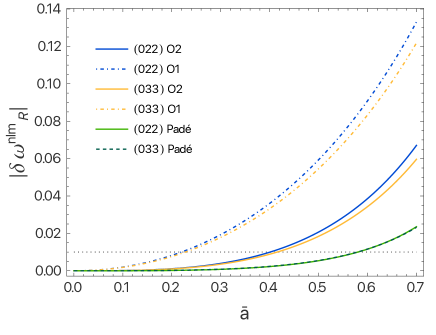
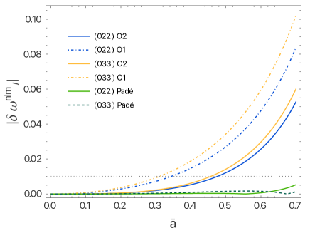
Figure 1: Real (upper panel) and imaginary (lower panel) parts of the relative difference between the QNMs of Kerr BHs and those of rotating BHs computed within the slow-rotation approximation, for the $(nlm)=(022),\,(033)$ modes. The slow-rotation expansion is performed to first order ($O1$), to second order ($O2$), to second order with Padé resummation (Padé). The horizontal dotted line represents a $1\%$ error.

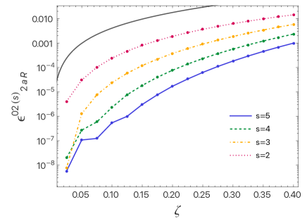
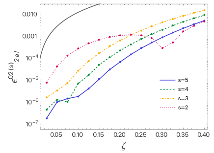
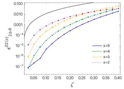
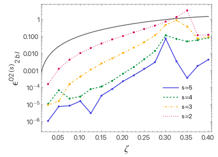
Figure 2: Truncation errors at order $s\leq 5$ for $\omega_{2a}(\zeta)$ (upper panels) and $\omega_{2b}(\zeta)$ (lower panels), for the $(nl)=(02)$ QNM. The real and imaginary parts are shown in left panels and right panels, respectively. The truncation error is always smaller than the relative correction due to gravity modifications (solid curves).

In Fig. 1 we show real and imaginary parts of the discrepancies (44) as functions of $\bar{a}$, for the QNMs with $(nlm)=(022)$ and $(nlm)=(033)$, which are expected to be the most excited in typical binary BH coalescences [62, 9, 63, 64]. The curves labeled $O1$, $O2$ show the discrepancies between the modes of Kerr BHs and those computed within the slow-rotation approximation, to $O(\bar{a})$ and to $O({\bar{a}}^{2})$, respectively. The curves labeled Padé show the discrepancies with the $O({\bar{a}}^{2})$ modes resummed using Padé approximants (see Sec. III.4). We see that at first order, the discrepancy of the Taylor expansion is smaller than $1\%$ as long as $\bar{a}\lesssim 0.22$. Including the second order correction, the discrepancy is smaller than $1\%$ for $\bar{a}\lesssim 0.4$. The Padé resummation improves the accuracy of the expansion, which is accurate to $\sim 1\%$ for $\bar{a}\lesssim 0.6$ and to $\sim 2\%$ for $\bar{a}\lesssim 0.7$.

An analysis of the modes with different values of $m$ shows the same (or better) accuracy for the Padé-resummed modes, but we need to employ the approximant $P[0,2]$ instead of $P[1,1]$ in two cases: the modes with $m=0$ (for which Eq. (42) reduces to a constant) and the imaginary parts of the modes with $m=\pm 1$.

These results (which are similar to those found in [59], with the exception of those for which we have used the $P[0,2]$ approximant, finding better accuracy) provide an indication that a second-order computation of QNMs may be accurate for $\bar{a}\lesssim 0.4$ ($\bar{a}\lesssim 0.7$ with Padé resummation) for EdGB gravity as well. In the following, then, we shall mostly consider values of the spin in the range $\bar{a}\in[0,0.7]$.

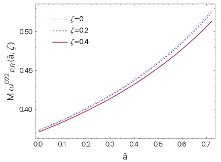
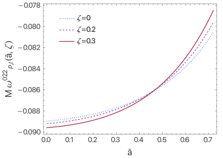
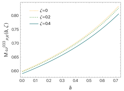
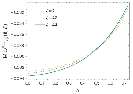
Figure 3: Real (upper panels) and imaginary (lower panels) parts of the $(nlm)=(022)$ (left panels) and $(nlm)=(033)$ (right panels) QNMs, evaluated using Padé approximants, as functions of the spin, for different values of $\zeta$.

Expansion in the coupling constant

To assess the accuracy of the expansion in the dimensionless coupling $\zeta$, we have computed the functions $\omega_{r}^{nl(s)}(\zeta)$ (40), by expanding the background and the perturbation equations up to order $s$ in $\zeta$ and up to second order in $\bar{a}$; we have repeated the computation for $s=2,\dots,6$, denoting the functions computed in this way as $\omega_{r}^{nl(s)}(\zeta)$. We then define the truncation error at order $s$ of $\omega_{r}^{nl}(\zeta)$ as:

$$\epsilon^{nl(s)}_{r\,R,I}(\zeta)=\frac{\left|\omega_{r\,R,I}^{nl(s+1)}(\zeta)-\omega_{r\,R,I}^{(s)}(\zeta)\right|}{\left|\omega_{r\,R,I}^{nl(s)}(\zeta)\right|}$$ (45)

where $r=0,1,2a,2b$ and the subscripts $R,I$ refer to the real and imaginary parts of the complex frequencies.

This analysis has been performed in Paper I to first order in the spin, i.e. for $r=0,1$. We here extend this computation to the the discrepancies of the $O({\bar{a}}^{2})$ contributions, i.e. for $r=2a$, $2b$. The truncation errors for these functions are shown in Fig. 2. We see that (as for $r=0,1$, see Paper I) the expansion in $\zeta$ is accurate within $1\%$ as long as $\zeta<0.4$ for the real parts of the modes, and $\zeta<0.3$ for the imaginary parts. Thus, in the rest of the paper we shall consider these ranges for the coupling $\zeta$. In Fig. 2 we also show the relative shift between the functions $\omega^{nl}_{r}$ in GR and in EdGB gravity; we can see that the truncation error $\epsilon^{nl(s)}_{r}$ at $s=5$ is significantly smaller than the EdGB contribution.

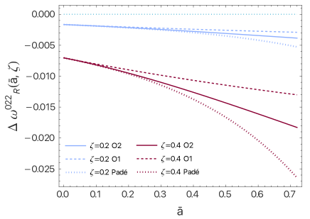
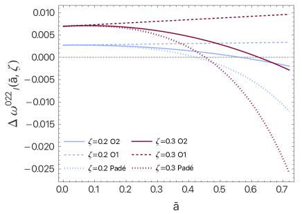
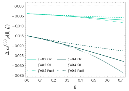
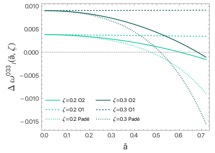
Figure 4: Real (left panels) and imaginary (right panels) parts of the relative difference of EdGB QNMs with respect to GR, as a function of $\bar{a}$. We consider the $(nlm)=(022)$ (upper panels) and $(nlm)=(033)$ (lower panels) QNMs computed up to the first order in the spin, up to second order, and with Padé resummation.

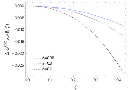
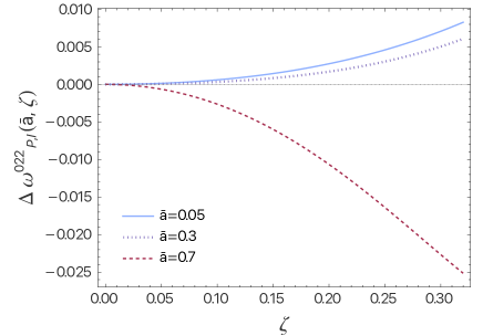
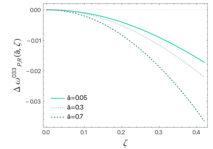
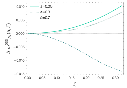
Figure 5: Same as Fig. 4, as a function of $\zeta$, with QNMs computed with Padé resummation.

IV.2 Quasi-normal modes

The Padé QNMs with $(nlm)=(022),\,(033)$ are shown in Fig. 3, as functions of the spin, for different values of $\zeta$. We can see that (for these modes) while at low values of the spin the EdGB corrections increase (in modulus) both the real and imaginary parts of the QNMs, when the spin is larger the EdGB correction increases the real parts of the modes, decreases the imaginary parts.

In order to undestand the effect of the EdGB corrections, it is useful to define the relative differences between the QNMs in EdGB gravity and in GR:

$$\Delta\omega^{nlm}_{R,I}(\bar{a},\zeta)=\frac{\omega^{nlm}_{R,I}(\bar{a},\zeta)-\omega^{nlm}_{R,I}(\bar{a},0)}{\omega^{nlm}_{R,I}(\bar{a},0)}$$ (46)

where $R,I$ refer to the real and imaginary parts, respectively. These quantities are shown in Fig. 4, for different values of $\zeta$, as functions of $\bar{a}$, and in Fig. 5 for different values of $\bar{a}$, as functions of $\zeta$. The spin expansion is performed to first and second order, and resummed using Padé approximants; in Fig. 5 it is only resummed using Padé approximants.

We note that (as argued in Paper I) the $O({\bar{a}^{2}})$ terms enhance the EdGB corrections to the QNMs; moreover, the corrections are further enhanced by the Padé resummation. For $\bar{a}=0.7$, the $l=2$ fundamental mode is shifted of $\sim 0.5\%$ for $\zeta=0.2$, and of $\sim 2.5\%$ for $\zeta=0.4$. We also note that the EdGB relative corrections of the imaginary parts change sign for large values of the spins; this explain the decreasing of the EdGB correction discussed above.

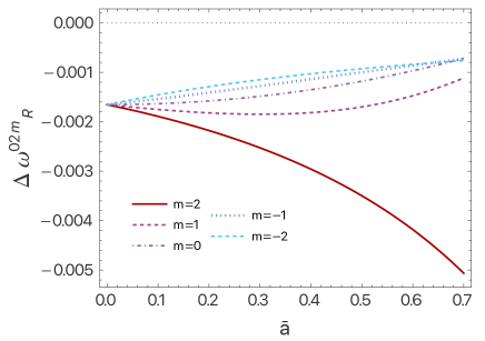
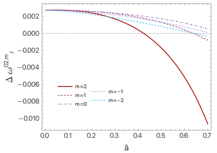
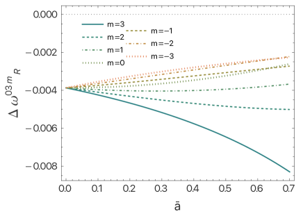
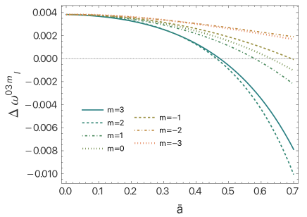
Figure 6: Real (upper panels) and imaginary (lower panels) of the relative difference of EdGB QNMs with respect to GR as a function of $\bar{a}$, for $\bar{\zeta}=0.2$ and different values of $m$. We consider $(nl)=(02)$ (left panels) and $(nl)=(03)$ (right panels) QNMs.

From Fig. 5 we note that when $\zeta\lesssim 0.3$, the contribution of the GR deviations to the QNMs is typically smaller than $2\%$, which is the error we expect from the slow-rotation expansion (see Fig. 1). Therefore, the slow-rotation expansion to $O({\bar{a}}^{2})$ discussed in this paper should only be used for the EdGB corrections ($O(\zeta^{2})$), while Kerr modes (or a slow-rotation expansion to a high order) should be used to compute the GR contribution ($O(\zeta^{0})$). In this way, the error due to the $O({\bar{a}}^{2})$ truncation would only affect the EdGB part of the modes. Finally, in Fig. 6 we show the EdGB relative corrections for the fundamental modes with $l=2,3$, for different values of $m$.

IV.3 Fits and Taylor expansions in the coupling constant

We have fitted the functions $\omega^{nl}_{r}(\zeta)$ defined in Eq. (40) with sixth-order polynomials in $\zeta$ ($\zeta\in[0.0.4]$ for the real parts, $\zeta\in[0,0.3]$ for the imaginary parts):

$$M\,\omega^{nl}_{r}(\zeta)=\sum_{i=0}^{6}\zeta^{i}C^{nl}_{r\,i}\,.$$ (47)

Since for gravitational-led modes the EdGB correction is of $O(\zeta^{2})$, we have set $C^{nl}_{r\,1}=0$ [19]. We have estimated the relative error of the fit (47), $\delta_{\rm f}$, as the mean over 100 attempts of the relative difference between the fit, computed from randomly selected $80\%$ of the data points, and the remaining $20\%$ of the data. For $l=3$ and $r=2a\,2b$, the functions have been fitted with fourth-order polynomials, because the error $\delta_{\rm f}$ is smaller.

In Tables 1-4 we show the coefficients of the fit (47) for the (gravitational-led, polar-led) fundamental modes with $l=2,3$. We also show the corresponding relative errors $\delta_{\rm f}$.

Table 1: Coefficients of the fit 47 of $\omega^{0l}_{r}$ for gravitational-led, polar-led modes, with $r=0$, $l=2,3$, up to $i=6$. In the last line we show the relative error of the fit, $\delta_{\rm f}$.

	Re (${l}=2$)	Im (${l}=2$)	Re (${l}=3$)	Im (${l}=3$)
$C_{0}$	0.37367	$-0.08896$	0.59944	$-0.09270$
$C_{2}$	$-1.406\cdot 10^{-2}$	$-4.70\cdot 10^{-3}$	$-5.453\cdot 10^{-2}$	$-7.19\cdot 10^{-3}$
$C_{3}$	$-7.53\cdot 10^{-3}$	$-6.10\cdot 10^{-3}$	$-3.093\cdot 10^{-2}$	$-1.098\cdot 10^{-2}$
$C_{4}$	$1.35\cdot 10^{-3}$	$-3.22\cdot 10^{-3}$	$6.419\cdot 10^{-2}$	$1.001\cdot 10^{-2}$
$C_{5}$	$7.09\cdot 10^{-3}$	$-1.61\cdot 10^{-3}$	$2.417\cdot 10^{-2}$	$2.158\cdot 10^{-2}$
$C_{6}$	$-2.03\cdot 10^{-3}$	$-2.8\cdot 10^{-4}$	$-5.215\cdot 10^{-2}$	$-3.345\cdot 10^{-2}$
$\delta_{\rm f}$	$2\cdot 10^{-9}$	$3\cdot 10^{-8}$	$10^{-7}$	$2\cdot 10^{-7}$

Table 2: As in Table 1, with $r=1$.

	Re (${l}=2$)	Im (${l}=2$)	Re (${l}=3$)	Im (${l}=3$)
$C_{0}$	0.06289	$0.00100$	0.06737	$0.00065$
$C_{2}$	$-1.048\cdot 10^{-2}$	$2\cdot 10^{-5}$	$-2.156\cdot 10^{-2}$	$1.18\cdot 10^{-3}$
$C_{3}$	$-1.074\cdot 10^{-2}$	$-2.69\cdot 10^{-3}$	$-2.056\cdot 10^{-2}$	$-3.19\cdot 10^{-3}$
$C_{4}$	$-1.53\cdot 10^{-3}$	$-9.86\cdot 10^{-3}$	$4.465\cdot 10^{-2}$	$3.9\cdot 10^{-4}$
$C_{5}$	$-2.40\cdot 10^{-3}$	$8.90\cdot 10^{-3}$	$2.341\cdot 10^{-2}$	$-1.224\cdot 10^{-2}$
$C_{6}$	$1.433\cdot 10^{-2}$	$-3.773\cdot 10^{-2}$	$-6.800\cdot 10^{-2}$	$1.056\cdot 10^{-2}$
$\delta_{\rm f}$	$5\cdot 10^{-8}$	$2\cdot 10^{-5}$	$10^{-6}$	$10^{-4}$

Table 3: As in Table  1, with $r=2a$. The fit for $l=3$ stops at fourth order in $\zeta$.

	Re (${l}=2$)	Im (${l}=2$)	Re (${l}=3$)	Im (${l}=3$)
$C_{0}$	0.03591	$0.00638$	0.04755	$0.00659$
$C_{2}$	$1.348\cdot 10^{-2}$	$6.50\cdot 10^{-3}$	$2.941\cdot 10^{-2}$	$1.857\cdot 10^{-2}$
$C_{3}$	$1.051\cdot 10^{-2}$	$8.48\cdot 10^{-3}$	$2.354\cdot 10^{-2}$	$8.93\cdot 10^{-3}$
$C_{4}$	$1.051\cdot 10^{-2}$	$5.06\cdot 10^{-3}$	$-2.391\cdot 10^{-2}$	$-2.78\cdot 10^{-3}$
$C_{5}$	$4.85\cdot 10^{-3}$	$1.402\cdot 10^{-2}$	$-$	$-$
$C_{6}$	$1.037\cdot 10^{-2}$	$-2.24\cdot 10^{-3}$	$-$	$-$
$\delta_{\rm f}$	$7\cdot 10^{-7}$	$2\cdot 10^{-6}$	$10^{-4}$	$10^{-3}$

Table 4: As in Table 3, with $r=2b$.

	Re (${l}=2$)	Im (${l}=2$)	Re (${l}=3$)	Im (${l}=3$)
$C_{0}$	0.00896	$-0.00031$	0.00661	$0.00006$
$C_{2}$	$-8.37\cdot 10^{-3}$	$3.13\cdot 10^{-3}$	$-9.95\cdot 10^{-3}$	$7.0\cdot 10^{-4}$
$C_{3}$	$-1.201\cdot 10^{-2}$	$2.95\cdot 10^{-3}$	$-4.90\cdot 10^{-3}$	$-2.27\cdot 10^{-3}$
$C_{4}$	$2.67\cdot 10^{-3}$	$-1.046\cdot 10^{-2}$	$4.78\cdot 10^{-3}$	$-1.57\cdot 10^{-3}$
$C_{5}$	$-5.926\cdot 10^{-2}$	$3.088\cdot 10^{-2}$	$-$	$-$
$C_{6}$	$8.254\cdot 10^{-2}$	$-6.819\cdot 10^{-2}$	$-$	$-$
$\delta_{\rm f}$	$5\cdot 10^{-6}$	$5\cdot 10^{-4}$	$2\cdot 10^{-4}$	$4\cdot 10^{-2}$

Table 5: Coefficients $\omega^{nl}_{r\,(A)}$ of the Taylor expansion (48), for the gravitational-led, polar-led fundamental ($n=0$) modes with $l=2,3$.

$r\,A$	Re (${l}=2$)	Im (${l}=2$)	Re (${l}=3$)	Im (${l}=3$)
$0\,0$	0.37367	$-0.08896$	0.59944	$-0.09270$
$1\,0$	$6.289\cdot 10^{-2}$	$1.00\cdot 10^{-3}$	$6.737\cdot 10^{-2}$	$6.5\cdot 10^{-4}$
$2a\,0$	$3.591\cdot 10^{-2}$	$6.38\cdot 10^{-3}$	$4.755\cdot 10^{-2}$	$6.59\cdot 10^{-3}$
$2b\,0$	$8.96\cdot 10^{-3}$	$-3.1\cdot 10^{-4}$	$6.61\cdot 10^{-3}$	$6\cdot 10^{-5}$
$r\,A$	Re (${l}=2$)	Im (${l}=2$)	Re (${l}=3$)	Im (${l}=3$)
$0\,2$	$-1.411\cdot 10^{-2}$	$-4.70\cdot 10^{-3}$	$-5.463\cdot 10^{-2}$	$-7.21\cdot 10^{-3}$
$1\,2$	$-1.049\cdot 10^{-2}$	$4\cdot 10^{-5}$	$-2.166\cdot 10^{-2}$	$1.17\cdot 10^{-3}$
$2a\,2$	$1.340\cdot 10^{-2}$	$6.54\cdot 10^{-3}$	$2.947\cdot 10^{-2}$	$1.777\cdot 10^{-2}$
$2b\,2$	$-8.42\cdot 10^{-3}$	$3.19\cdot 10^{-3}$	$-9.50\cdot 10^{-3}$	$4.3\cdot 10^{-4}$

These fits are very accurate to describe the functions $\omega^{nl}_{r}(\zeta)$ in the entire range $\zeta\in[0,0.4]$ ($[0,0.3]$ for the imaginary parts). If we are interested in these functions for $\zeta\ll 1$, we should instead compute a Taylor expansion of them around $\zeta=0$. A Taylor expansion is also useful for data analysis techniques based on QNM expansions in the spin, like ParSpec  [10, 65, 66]. Therefore, we performed a Taylor expansion of the functions $\omega^{nl}_{r}(\zeta)$ to $O(\zeta^{2})$:

$$\omega^{nl}_{r}(\zeta)=\omega^{nl}_{r\,(0)}+\zeta^{2}\omega^{nl}_{r\,(2)}+O(\zeta^{3})$$ (48)

(as mentioned above, since we are considering gravitational-led modes, the first-order contributions $\omega^{nl}_{r\,(1)}$ identically vanish). The coefficients of the expansion (48), for the $(nl)=(02),\,(03)$ modes, are given in Table 5.

V Conclusions and outlook

In this article we have computed the QNMs of a rotating BH in EdGB gravity. Strictly speaking, this is a slow-rotation computation, since it is based on an expansion in the spin $\bar{a}$ up to second order. However, the use of Padé approximants enhances the range of validity of the expansion: an analysis of the general relativistic case suggests that the QNMs derived with this approach are accurate within $\sim 2\%$ up to phenomenologically relevant values of the spin, i.e. for $\bar{a}\lesssim 0.7$ (see also [59]).

We find that (as argued in Paper I) the second-order contribution greatly enhances the EdGB correction to the QNMs. For instance, for the real part of the $(nlm)=(022)$ – which is the mode typically excited with largest amplitude in actual BH ringdowns (see e.g. [64]) – , assuming a BH spin of $\bar{a}=0.7$, the EdGB correction estimated to $O(\bar{a})$ for $\zeta\simeq 0.4$ ($\zeta\simeq 0.3$ for the imaginary part) is of $\simeq 1\%$, while that estimated to $O({\bar{a}}^{2})$ (with Padé resummation) is of $\simeq 2.5\%$ (see Fig. 5).

Our computation has been performed expanding the background and the perturbation equations in the coupling constant to $O(\zeta^{6})$. An analysis of the truncation error indicates that our results are accurate for $\zeta\lesssim 0.4$ for the real parts of the modes, $\zeta\lesssim 0.3$ for the imaginary parts. We provide analytical fits of the modes in this range of the coupling constant. We also provide a Taylor expansion around $\zeta=0$, which can be useful in the data analysis of ringdown signals.

Concerning the detectability of the EdGB deviations, we note that $O(10)$ detections of binary BH ringdowns with signal-to-noise ratios (SNRs) of the order of $\sim 30$ are expected to be sufficient to measure BH QNMs with an accuracy of few percent (see e.g. [67]). Since third-generation detectors, like the Einstein Telescope [4], are expected to reach even larger SNRs, they could be sensitive enough to find the deviations studied in this article, at least for the largest values of the coupling. This, however, is just an order-of-magnitude estimate: in order to assess the detectabilty of EdGB corrections in the BH QNMs by third-generation detectors we need to know the SNR and the number of events required to measure the EdGB shifts, as functions of the coupling constant. This can only be found with a proper sensitivity analysis of the combined detections of several oscillating BHs, with different masses and spins. Such analysis, based on the ParSpec framework [10], is currently in preparation [66].

This is the first computation, in a modified gravity theory, of the QNMs of BHs to second order in rotation. Although EdGB gravity is an interesting theory by itself for a number of reasons, this can also be considered as a study case, to understand which kind of deviation we may expect in the ringdown signal. The mode corrections in specific theories of gravity are a necessary ingredient of gravitational spectroscopy, using future GW data to perform tests of gravity which go beyond null tests of GR [10, 65, 66]. Of course, the next step will to extend this computation to other classes of possible GR deviations.

The computation presented here will also be useful, once fully numerical simulations of BH coalescences in EdGB gravity will be available [36, 68, 69, 70], as a benchmark to test the numerical codes.

Appendix A Equations for gravitational perturbations at second order in the spin

The field equations (2), (3), linearized in the perturbation around the stationary BH solution discussed in Sec. II, can be written as follows (we follow the same notation as [49], and leave implicit the sum over $l,m$):

$$\left[A^{(I)}_{lm}+\tilde{A}^{(I)}_{lm}\cos\theta+\hat{A}^{(I)}_{lm}\cos^{2}\theta\right]Y(\theta)+im\left[C^{(I)}_{lm}+\tilde{C}^{(I)}_{lm}\cos\theta\right]Y^{lm}(\theta)+m^{2}E^{(I)}_{lm}Y^{lm}(\theta)$$

$$+\left[B^{(I)}_{lm}+\tilde{B}^{(I)}_{lm}\cos\theta+imD^{(I)}_{lm}\right]\ \sin\theta\ {Y^{\prime}}^{lm}(\theta) =0\,,$$ (49)

$$\left[\alpha^{(J)}_{lm}+\tilde{\alpha}^{(J)}_{lm}\cos\theta+\hat{\alpha}^{(J)}_{lm}\cos^{2}\theta\right]\sin\theta\ {Y}^{lm}(\theta)_{,\theta}-im\left[\beta^{(J)}_{lm}+\tilde{\beta}^{(J)}_{lm}\cos\theta+\hat{\beta}^{(J)}_{lm}\cos^{2}\theta\right]Y^{lm}(\theta)$$

$$+\left[\eta^{(J)}_{lm}+\tilde{\eta}^{(J)}_{lm}\cos\theta\right]\sin^{2}\theta Y^{lm}(\theta)+\left[\xi^{(J)}_{lm}+\tilde{\xi}^{(J)}_{lm}\cos\theta\right]\sin\theta X^{lm}(\theta)+\left[\gamma^{(J)}_{lm}+\tilde{\gamma}^{(J)}_{lm}cos\theta\right]\sin^{2}\theta W^{lm}(\theta) =0\,$$ (50)

$$-\left[\beta^{(J)}_{lm}+\tilde{\beta}^{(J)}_{lm}cos\theta+\hat{\beta}^{(J)}_{lm}\cos^{2}\theta+\tilde{\Delta}^{(J)}_{lm}\sin^{2}\theta\right]\sin\theta\ {Y}^{lm}(\theta)_{,\theta}$$

$$-im\left[\alpha^{(J)}_{lm}+\tilde{\alpha}^{(J)}_{lm}\cos\theta+\hat{\alpha}^{(J)}_{lm}\cos^{2}\theta+\Delta^{(J)}_{lm}\sin^{2}\theta\right]Y^{lm}(\theta)-\left[\zeta^{(J)}_{lm}+\tilde{\zeta}^{(J)}_{lm}\cos\theta\right]\sin^{2}\theta\ Y^{lm}(\theta)$$

$$-\left[\gamma^{(J)}_{lm}l+\tilde{\gamma}^{(J)}_{lm}\cos\theta\right]\sin\theta X^{lm}(\theta)+\left[\xi^{(J)}_{lm}+\tilde{\xi}^{(J)}_{lm}\cos\theta\right]\sin^{2}\theta W^{lm}(\theta) =0\,,$$ (51)

$$\left[f_{lm}+\tilde{f}_{lm}\cos\theta\right]\sin\theta\ {Y}^{lm}(\theta)_{,\theta}+im\left[g_{lm}+\tilde{g}_{lm}\cos\theta\right]Y^{lm}(\theta)+k_{lm}\sin^{2}\theta\ Y^{lm}(\theta)$$

$$+\left[s_{lm}+\hat{s}_{lm}\cos^{2}\theta\right]\frac{X^{lm}(\theta)}{\sin\theta}+\left[t_{lm}+\hat{t}_{lm}\cos^{2}\theta\right]W^{lm}(\theta)= 0\,,$$ (52)

$$\left[g_{lm}+\tilde{g}_{lm}\cos\theta\right]\sin\theta\ {Y}^{lm}(\theta)_{,\theta}-im\left[f_{lm}+\tilde{f}_{lm}\cos\theta\right]Y^{lm}(\theta)+\hat{k}_{lm}\sin^{2}\theta\ Y^{lm}(\theta)$$

$$-\left[t_{lm}+\hat{t}_{lm}\cos^{2}\theta\right]\frac{X^{lm}(\theta)}{\sin\theta}+\left[s_{lm}+\hat{s}_{lm}\cos^{2}\theta\right]W^{lm}(\theta) =0\,,$$ (53)

where in Eq. (49), $I=0,1,2,3$ correspond to the components of Einstein’s field equations behaving as scalars under rotations, and $I=4$ corresponds to the scalar field equation; $J=0,1$ in Eqs. (50), (51) correspond to the components of Einstein’s field equations behaving as vectors under rotations; and Eqs. (52), (53), correspond to the components of Einstein’s field equations behaving as rank-two tensors under rotations. We have defined

$$X^{lm}(\theta,\varphi)\equiv 2Y^{lm}_{,\theta\varphi}-2\frac{\cos\theta}{\sin\theta}Y^{lm}_{,\varphi}$$ (54)

$$W^{lm}(\theta,\varphi)\equiv-2\frac{\cos\theta}{\sin\theta}Y_{,\theta}-l(l+1)Y^{lm}-2\frac{Y^{lm}_{,\varphi\varphi}}{\sin^{2}\theta}\,.$$ (55)

The coefficients

• $A^{(I)}_{lm}$, $\alpha^{(J)}_{lm}$, $\beta^{(J)}_{lm}$, $s_{lm}$, $t_{lm}$ contain both zero-th order and second order in the spin terms;

• ${\tilde{A}}^{(I)}_{lm}$, $C^{(I)}_{lm}$, $B^{(I)}_{lm}$, ${\tilde{\alpha}}^{(J)}_{lm}$, ${\tilde{\beta}}^{(J)}_{lm}$, ${\eta}^{(J)}_{lm}$, ${\xi}^{(J)}_{lm}$, ${\gamma}^{(J)}_{lm}$, ${\zeta}^{(J)}_{lm}$, $f_{lm}$, $g_{lm}$ are of order $O({\bar{a}})$;

• ${\hat{A}}^{(J)}_{lm}$, ${\tilde{C}}^{(J)}_{lm}$, ${E}^{(J)}_{lm}$, ${\tilde{B}}^{(J)}_{lm}$, ${D}^{(J)}_{lm}$, ${\hat{\alpha}}^{(J)}_{lm}$, ${\hat{\beta}}^{(J)}_{lm}$, ${\tilde{\eta}}^{(J)}_{lm}$, ${\tilde{\xi}}^{(J)}_{lm}$, ${\tilde{\gamma}}^{(J)}_{lm}$,${\tilde{\zeta}}^{(J)}_{lm}$, ${\Delta}^{(J)}_{lm}$, ${\tilde{\Delta}}^{(J)}_{lm}$, ${\tilde{f}}^{(J)}_{lm}$, ${\tilde{g}}^{(J)}_{lm}$, ${k}^{(J)}_{lm}$, ${\hat{k}}^{(J)}_{lm}$, ${\hat{s}}^{(J)}_{lm}$, ${\hat{t}}^{(J)}_{lm}$ are of the second order in the spin.

All of them are linear combinations of the perturbation functions $h^{lm}_{0}(r)$, $h^{lm}_{1}(r)$, $H^{lm}_{0}(r)$, $H^{lm}_{1}(r)$, $H^{lm}_{2}(r)$, $K^{lm}(r)$, $\Phi^{lm}(r)$ and their derivatives, with coefficients that depend on $l$ but not on $m$. Their explicit expansions in the coupling parameter $\zeta$, up to $O(\zeta^{6})$, are given in the Supplemental Material [46].

We project Eqs. (49)-(53) on the complete set of tensor spherical harmonics, as in [49], decoupling the angular variables:

$$A^{(I)}_{lm}+\hat{A}^{(I)}_{lm}\left[Q_{lm}^{2}+Q_{l+1\,m}^{2}\right]+\tilde{B}^{(I)}_{lm}\left[lQ^{2}_{l+1\,m}-(l+1)Q^{2}_{lm}\right]+imC^{(I)}_{lm}+m^{2}E^{(I)}_{lm}+Q_{lm}\Big{\{}\left[\tilde{A}^{(I)}_{l-1\,m}+(l-1)B^{(I)}_{l-1\,m}\right]$$

$$+im\left[\tilde{C}^{(I)}_{l-1\,m}+(l-1)D^{(I)}_{l-1\,m}\right]\Big{\}}+Q_{l+1\,m}\Big{\{}\left[\tilde{A}^{(I)}_{l+1\,m}-(l+2)B^{(I)}_{l+1\,m}\right]+im\left[\tilde{C}^{(I)}_{l+1\,m}-(l+2)D^{(I)}_{l+1\,m}\right]\Big{\}}$$

$$+Q_{lm}Q_{l-1\,m}\left[\hat{A}^{(I)}_{l-2\,m}+(l-2)\tilde{B}^{(I)}_{l-2\,m}\right]+Q_{l+1\,m}Q_{l+2\,m}\left[\hat{A}_{l+2\,m}^{(I)}-(l+3)\tilde{B}^{(I)}_{l+2\,m}\right]=0\,,$$ (56)

$$l(l+1)\alpha^{(J)}_{lm}-im\left[\tilde{\beta}^{(J)}_{lm}+\zeta^{(J)}_{lm}-(l-1)(l+2)\xi^{(J)}_{lm}\right]+\left[(l+1)(l-2)Q_{lm}^{2}+l(l+3)Q^{2}_{l+1\,m}\right]\hat{\alpha}^{(J)}_{lm}$$

$$+m^{2}\Delta^{(J)}_{lm}+\left[lQ^{2}_{l+1\,m}-(l+1)Q_{lm}^{2}\right]\tilde{\eta}^{(J)}_{lm}+\left[2m^{2}+Q^{2}_{lm}(l+1)(l^{2}-l+4)-Q^{2}_{l+1\,m}l(l^{2}+3l+6)\right]\tilde{\gamma}^{(J)}_{lm}$$

$$+Q_{lm}\Big{\{}(l-1)(l+1)\tilde{\alpha}^{(J)}_{l-1\,m}-(l+1)\eta^{(J)}_{l-1\,m}+(l-2)(l-1)(l+1)\gamma^{(J)}_{l-1\,m}$$

$$\ \ \ \ -im\left[2\hat{\beta}^{(J)}_{l-1\,m}+(l-1)\tilde{\Delta}^{(J)}_{l-1\,m}+\tilde{\zeta}^{(J)}_{l-1\,m}-(l-2)(l+3)\tilde{\xi}^{(J)}_{l-1\,m}\right]\Big{\}}$$

$$+Q_{l+1\,m}\Big{\{}l(l+2)\tilde{\alpha}^{(J)}_{l+1\,m}+l\eta^{(J)}_{l+1\,m}-l(l+2)(l+3)\gamma^{(J)}_{l+1\,m}$$

$$\ \ \ \ -im\left[2\hat{\beta}^{(J)}_{l+1\,m}-(l+2)\tilde{\Delta}^{(J)}_{l+1\,m}+\tilde{\zeta}^{(J)}_{l+1\,m}-(l-2)(l+3)\tilde{\xi}^{(J)}_{l+1\,m}\right]\Big{\}}$$

$$+Q_{l-1\,m}Q_{lm}\Big{\{}(l-2)(l+1)\hat{\alpha}^{(J)}_{l-2\,m}-(l+1)\tilde{\eta}^{(J)}_{l-2\,m}+(l-2)(l+1)(l-3)\tilde{\gamma}^{(J)}_{l-2\,m}\Big{\}}$$

$$+Q_{l+1\,m}Q_{l+2\,m}\Big{\{}l(l+3)\hat{\alpha}^{(J)}_{l+2}+l\tilde{\eta}_{l+2\,m}^{(J)}-l(l+3)(l+4)\ \tilde{\gamma}^{(J)}_{l+2\,m)}\Big{\}}=0\,,$$ (57)

$$l(l+1)\beta^{(J)}_{lm}+im\left[\tilde{\alpha}^{(J)}_{lm}+\eta^{(J)}_{lm}+(l-1)(l+2)\gamma^{(J)}_{lm}\right]+\left[(l+1)(l-2)Q_{lm}^{2}+l(l+3)Q^{2}_{l+1\,m}\right]\hat{\beta}^{(J)}_{lm}+\big{[}l^{2}Q^{2}_{l+1\,m}$$

$$+(l+1)^{2}Q_{lm}^{2}\big{]}\tilde{\Delta}^{(J)}_{lm}+\left[lQ^{2}_{l+1\,m}-(l+1)Q_{lm}^{2}\right]\tilde{\zeta}^{(J)}_{lm}-\left[2m^{2}+Q^{2}_{lm}(l+1)(l^{2}-l+4)-Q^{2}_{l+1\,m}l(l^{2}+3l+6)\right]\tilde{\xi}^{(J)}_{lm}$$

$$+Q_{lm}\Big{\{}(l-1)(l+1)\tilde{\beta}^{(J)}_{l-1\,m}-(l+1)\zeta^{(J)}_{l-1\,m}-(l-2)(l-1)(l+1)\xi^{(J)}_{l-1\,m}$$

$$\ \ \ \ +im\left[2\hat{\alpha}^{(J)}_{l-1\,m}-(l+1)\Delta^{(J)}_{l-1\,m}+\tilde{\eta}^{(J)}_{l-1\,m}+(l-2)(l+3)\tilde{\gamma}^{(J)}_{l-1\,m}\right]\Big{\}}$$

$$+Q_{l+1\,m}\Big{\{}l(l+2)\tilde{\beta}^{(J)}_{l+1\,m}+l\zeta^{(J)}_{l+1\,m}+l(l+2)(l+3)\xi^{(J)}_{l+1\,m}+im\left[2\hat{\alpha}^{(J)}_{l+1\,m}+l\Delta^{(J)}_{l+1\,m}+\tilde{\eta}^{(J)}_{l+1\,m}+(l-2)(l+3)\tilde{\gamma}^{(J)}_{l+1\,m}\right]\Big{\}}$$

$$+Q_{l-1\,m}Q_{lm}\Big{\{}(l-2)(l+1)\hat{\beta}^{(J)}_{l-2\,m}-(l+1)\tilde{\zeta}^{(J)}_{l-2\,m}-(l-2)(l+1)(l-3)\tilde{\xi}^{(J)}_{l-2\,m}-(l-2)(l+1)\tilde{\Delta}^{(J)}_{l-2\,m}\Big{\}}$$

$$+Q_{l+1\,m}Q_{l+2\,m}\Big{\{}l(l+3)\hat{\beta}^{(J)}_{l+2\,m}+l\tilde{\zeta}_{l+2\,m}^{(J)}+l(l+3)(l+4)\tilde{\xi}^{(J)}_{l+2\,m}-l(l+3)\tilde{\Delta}^{(J)}_{l+2\,m}\Big{\}}=0\,,$$ (58)

$$l(l-1)(l+1)(l+2)s_{lm}-im(l-1)(l+2)f_{lm}+\left[2m^{2}+Q_{lm}^{2}(l+1)(l^{2}-l+4)-Q^{2}_{l+1\,m}l(l^{2}+3l+6)\right]\tilde{g}_{lm}$$

$$+\left[2m^{2}-l(l+1)+(l+1)(l+2)Q_{lm}^{2}+l(l-1)Q^{2}_{l+1\,m}\right]\hat{k}_{lm}$$

$$+\Big{\{}8m^{2}-2l(l+1)-Q_{lm}^{2}(l+1)\left[4(l-2)-l(l+1)(l+4)\right]-Q_{l+1\,m}^{2}l\left[4(l+3)-l(l+1)(l-3)\right]\Big{\}}\hat{s}_{lm}$$

$$-Q_{lm}\Big{\{}(l-1)(l+1)(l+2)g_{l-1\,m}+im\left[(l-3)(l+2)\tilde{f}_{l-1\,m}-2(l+2)k_{l-1\,m}+4(l-2)(l+2)\hat{t}_{l-1\,m}\right]\Big{\}}$$

$$+Q_{l+1\,m}\Big{\{}l(l-1)(l+2)g_{l+1\,m}-im\left[(l-1)(l+4)\tilde{f}_{l+1\,m}+2(l-1)k_{l+1\,m}+4(l-1)(l+3)\hat{t}_{l+1\,m}\right]\Big{\}}$$

$$+Q_{l-1\,m}Q_{lm}(l+1)(l+2)\Big{\{}-(l-2)\tilde{g}_{l-2\,m}+\hat{k}_{l-2\,m}+(l-3)(l-2)\hat{s}_{l-2\,m}\Big{\}}$$

$$+Q_{l+1\,m}Q_{l+2\,m}l(l-1)\Big{\{}(l+3)\tilde{g}_{l+2\,m}+\hat{k}_{l+2\,m}+(l+3)(l+4)\hat{s}_{l+2\,m}\Big{\}}=0\,,$$ (59)

$$0=l(l-1)(l+1)(l+2)t_{l}+im(l-1)(l+2)g_{lm}+\left[2m^{2}+Q_{lm}^{2}(l+1)(l^{2}-l+4)-Q^{2}_{l+1\,m}l(l^{2}+3l+6)\right]\tilde{f}_{lm}$$

$$+\left[2m^{2}-l(l+1)+(l+1)(l+2)Q_{lm}^{2}+l(l-1)Q^{2}_{l+1\,m}\right]k_{lm}$$

$$+\Big{\{}8m^{2}-2l(l+1)-Q_{lm}^{2}(l+1)\left[4(l-2)-l(l+1)(l+4)\right]-Q_{l+1\,m}^{2}l\left[4(l+3)-l(l+1)(l-3)\right]\Big{\}}\hat{t}_{lm}$$

$$-Q_{lm}\Big{\{}(l-1)(l+1)(l+2)f_{l-1\,m}-im\left[(l-3)(l+2)\tilde{g}_{l-1\,m}-2(l+2)\hat{k}_{l-1\,m}+4(l-2)(l+2)\hat{s}_{l-1\,m}\right]\Big{\}}$$

$$+Q_{l+1\,m}\Big{\{}l(l-1)(l+2)f_{l+1}+im\left[(l-1)(l+4)\tilde{g}_{l+1\,m}+2(l-1)\hat{k}_{l+1\,m}+4(l-1)(l+3)\hat{s}_{l+1\,m}\right]\Big{\}}$$

$$+Q_{l-1\,m}Q_{lm}(l+1)(l+2)\Big{\{}-(l-2)\tilde{f}_{l-2\,m}+k_{l-2\,m}+(l-3)(l-2)\hat{t}_{l-2\,m}\Big{\}}$$

$$+Q_{l+1\,m}Q_{l+2\,m}l(l-1)\Big{\{}(l+3)\tilde{f}_{l+2\,m}+k_{l+2\,m}+(l+3)(l+4)\hat{t}_{l+2\,m}\Big{\}}\,,$$ (60)

where $l\geq 2$ and

$$Q_{lm}=\sqrt{\frac{(l-m)(l+m)}{(2l-1)(2l+1)}}\,.$$ (61)

As discussed in Sec. III.3, for polar-led perturbations with $l=2$ some of the terms in Eqs. (56) - (60) vanish, thus they reduce to Eqs. (29)-(35).

References

- [1] C. M. Will, “The Confrontation between General Relativity and Experiment,” Living Rev. Rel. 17 (2014) 4, arXiv:1403.7377 [gr-qc].
- [2] LIGO Scientific, Virgo Collaboration, B. P. Abbott et al., “Observation of Gravitational Waves from a Binary Black Hole Merger,” Phys. Rev. Lett. 116 no. 6, (2016) 061102, arXiv:1602.03837 [gr-qc].
- [3] LIGO Scientific, VIRGO, KAGRA Collaboration, R. Abbott et al., “Tests of General Relativity with GWTC-3,” arXiv:2112.06861 [gr-qc].
- [4] M. Punturo et al., “The Einstein Telescope: A third-generation gravitational wave observatory,” Class. Quant. Grav. 27 (2010) 194002.
- [5] K. D. Kokkotas and B. G. Schmidt, “Quasinormal modes of stars and black holes,” Living Rev. Rel. 2 (1999) 2, arXiv:gr-qc/9909058.
- [6] V. Ferrari and L. Gualtieri, “Quasi-Normal Modes and Gravitational Wave Astronomy,” Gen. Rel. Grav. 40 (2008) 945–970, arXiv:0709.0657 [gr-qc].
- [7] E. Berti, V. Cardoso, and A. O. Starinets, “Quasinormal modes of black holes and black branes,” Class. Quant. Grav. 26 (2009) 163001, arXiv:0905.2975 [gr-qc].
- [8] J. Meidam, M. Agathos, C. Van Den Broeck, J. Veitch, and B. S. Sathyaprakash, “Testing the no-hair theorem with black hole ringdowns using TIGER,” Phys. Rev. D 90 no. 6, (2014) 064009, arXiv:1406.3201 [gr-qc].
- [9] H. Yang, K. Yagi, J. Blackman, L. Lehner, V. Paschalidis, F. Pretorius, and N. Yunes, “Black hole spectroscopy with coherent mode stacking,” Phys. Rev. Lett. 118 no. 16, (2017) 161101, arXiv:1701.05808 [gr-qc].
- [10] A. Maselli, P. Pani, L. Gualtieri, and E. Berti, “Parametrized ringdown spin expansion coefficients: a data-analysis framework for black-hole spectroscopy with multiple events,” Phys. Rev. D 101 no. 2, (2020) 024043, arXiv:1910.12893 [gr-qc].
- [11] O. Dreyer, B. J. Kelly, B. Krishnan, L. S. Finn, D. Garrison, and R. Lopez-Aleman, “Black hole spectroscopy: Testing general relativity through gravitational wave observations,” Class. Quant. Grav. 21 (2004) 787–804, arXiv:gr-qc/0309007.
- [12] E. Berti, V. Cardoso, and C. M. Will, “On gravitational-wave spectroscopy of massive black holes with the space interferometer LISA,” Phys. Rev. D 73 (2006) 064030, arXiv:gr-qc/0512160.
- [13] E. Berti, J. Cardoso, V. Cardoso, and M. Cavaglia, “Matched-filtering and parameter estimation of ringdown waveforms,” Phys. Rev. D 76 (2007) 104044, arXiv:0707.1202 [gr-qc].
- [14] E. Berti, K. Yagi, H. Yang, and N. Yunes, “Extreme Gravity Tests with Gravitational Waves from Compact Binary Coalescences: (II) Ringdown,” Gen. Rel. Grav. 50 no. 5, (2018) 49, arXiv:1801.03587 [gr-qc].
- [15] V. Cardoso and L. Gualtieri, “Perturbations of Schwarzschild black holes in Dynamical Chern-Simons modified gravity,” Phys. Rev. D 80 (2009) 064008, arXiv:0907.5008 [gr-qc]. [Erratum: Phys.Rev.D 81, 089903 (2010)].
- [16] C. Molina, P. Pani, V. Cardoso, and L. Gualtieri, “Gravitational signature of Schwarzschild black holes in dynamical Chern-Simons gravity,” Phys. Rev. D 81 (2010) 124021, arXiv:1004.4007 [gr-qc].
- [17] T. Kobayashi, H. Motohashi, and T. Suyama, “Black hole perturbation in the most general scalar-tensor theory with second-order field equations I: the odd-parity sector,” Phys. Rev. D 85 (2012) 084025, arXiv:1202.4893 [gr-qc]. [Erratum: Phys.Rev.D 96, 109903 (2017)].
- [18] T. Kobayashi, H. Motohashi, and T. Suyama, “Black hole perturbation in the most general scalar-tensor theory with second-order field equations II: the even-parity sector,” Phys. Rev. D 89 no. 8, (2014) 084042, arXiv:1402.6740 [gr-qc].
- [19] J. L. Blázquez-Salcedo, C. F. B. Macedo, V. Cardoso, V. Ferrari, L. Gualtieri, F. S. Khoo, J. Kunz, and P. Pani, “Perturbed black holes in einstein-dilaton-gauss-bonnet gravity: Stability, ringdown, and gravitational-wave emission,” Phys. Rev. D 94 (Nov, 2016) 104024. https://link.aps.org/doi/10.1103/PhysRevD.94.104024.
- [20] O. J. Tattersall, “Quasi-Normal Modes of Hairy Scalar Tensor Black Holes: Odd Parity,” Class. Quant. Grav. 37 no. 11, (2020) 115007, arXiv:1911.07593 [gr-qc].
- [21] J. L. Blázquez-Salcedo, D. D. Doneva, S. Kahlen, J. Kunz, P. Nedkova, and S. S. Yazadjiev, “Polar quasinormal modes of the scalarized Einstein-Gauss-Bonnet black holes,” Phys. Rev. D 102 no. 2, (2020) 024086, arXiv:2006.06006 [gr-qc].
- [22] J. L. Blázquez-Salcedo, F. S. Khoo, and J. Kunz, “Quasinormal modes of Einstein-Gauss-Bonnet-dilaton black holes,” Phys. Rev. D 96 no. 6, (2017) 064008, arXiv:1706.03262 [gr-qc].
- [23] L. Pierini and L. Gualtieri, “Quasi-normal modes of rotating black holes in Einstein-dilaton Gauss-Bonnet gravity: the first order in rotation,” Phys. Rev. D 103 (2021) 124017, arXiv:2103.09870 [gr-qc].
- [24] P. Wagle, N. Yunes, and H. O. Silva, “Quasinormal modes of slowly-rotating black holes in dynamical Chern-Simons gravity,” arXiv:2103.09913 [gr-qc].
- [25] M. Srivastava, Y. Chen, and S. Shankaranarayanan, “Analytical computation of quasinormal modes of slowly rotating black holes in dynamical Chern-Simons gravity,” Phys. Rev. D 104 no. 6, (2021) 064034, arXiv:2106.06209 [gr-qc].
- [26] P. A. Cano, K. Fransen, T. Hertog, and S. Maenaut, “Gravitational ringing of rotating black holes in higher-derivative gravity,” Phys. Rev. D 105 no. 2, (2022) 024064, arXiv:2110.11378 [gr-qc].
- [27] V. Cardoso, M. Kimura, A. Maselli, E. Berti, C. F. B. Macedo, and R. McManus, “Parametrized black hole quasinormal ringdown: Decoupled equations for nonrotating black holes,” Phys. Rev. D 99 no. 10, (2019) 104077, arXiv:1901.01265 [gr-qc].
- [28] R. McManus, E. Berti, C. F. B. Macedo, M. Kimura, A. Maselli, and V. Cardoso, “Parametrized black hole quasinormal ringdown. II. Coupled equations and quadratic corrections for nonrotating black holes,” Phys. Rev. D 100 no. 4, (2019) 044061, arXiv:1906.05155 [gr-qc].
- [29] S. H. Völkel, N. Franchini, and E. Barausse, “Theory-agnostic reconstruction of potential and couplings from quasinormal modes,” Phys. Rev. D 105 no. 8, (2022) 084046, arXiv:2202.08655 [gr-qc].
- [30] E. Berti et al., “Testing General Relativity with Present and Future Astrophysical Observations,” Class. Quant. Grav. 32 (2015) 243001.
- [31] S. Mignemi and N. R. Stewart, “Charged black holes in effective string theory,” Phys. Rev. D 47 (1993) 5259–5269, arXiv:hep-th/9212146.
- [32] P. Kanti, N. E. Mavromatos, J. Rizos, K. Tamvakis, and E. Winstanley, “Dilatonic black holes in higher curvature string gravity,” Phys. Rev. D54 (1996) 5049–5058.
- [33] G. W. Horndeski, “Second-order scalar-tensor field equations in a four-dimensional space,” Int. J. Theor. Phys. 10 (1974) 363–384.
- [34] T. Kobayashi, “Horndeski theory and beyond: a review,” Rept. Prog. Phys. 82 no. 8, (2019) 086901, arXiv:1901.07183 [gr-qc].
- [35] S. E. Perkins, R. Nair, H. O. Silva, and N. Yunes, “Improved gravitational-wave constraints on higher-order curvature theories of gravity,” Phys. Rev. D 104 no. 2, (2021) 024060, arXiv:2104.11189 [gr-qc].
- [36] H. Witek, L. Gualtieri, P. Pani, and T. P. Sotiriou, “Black holes and binary mergers in scalar Gauss-Bonnet gravity: scalar field dynamics,” Phys. Rev. D 99 no. 6, (2019) 064035, arXiv:1810.05177 [gr-qc].
- [37] J. B. Hartle and K. S. Thorne, “Slowly Rotating Relativistic Stars. II. Models for Neutron Stars and Supermassive Stars,” Astrophys. J. 153 (1968) 807.
- [38] P. Pani, V. Cardoso, L. Gualtieri, E. Berti, and A. Ishibashi, “Perturbations of slowly rotating black holes: massive vector fields in the Kerr metric,” Phys. Rev. D 86 (2012) 104017, arXiv:1209.0773 [gr-qc].
- [39] P. Pani, E. Berti, and L. Gualtieri, “Gravitoelectromagnetic Perturbations of Kerr-Newman Black Holes: Stability and Isospectrality in the Slow-Rotation Limit,” Phys. Rev. Lett. 110 no. 24, (2013) 241103, arXiv:1304.1160 [gr-qc].
- [40] P. Pani and V. Cardoso, “Are black holes in alternative theories serious astrophysical candidates? The Case for Einstein-Dilaton-Gauss-Bonnet black holes,” Phys. Rev. D79 (2009) 084031.
- [41] T. P. Sotiriou and S.-Y. Zhou, “Black hole hair in generalized scalar-tensor gravity: An explicit example,” Phys. Rev. D 90 (2014) 124063, arXiv:1408.1698 [gr-qc].
- [42] N. Yunes and L. C. Stein, “Non-Spinning Black Holes in Alternative Theories of Gravity,” Phys. Rev. D 83 (2011) 104002, arXiv:1101.2921 [gr-qc].
- [43] B. Kleihaus, J. Kunz, and E. Radu, “Rotating Black Holes in Dilatonic Einstein-Gauss-Bonnet Theory,” Phys. Rev. Lett. 106 (2011) 151104, arXiv:1101.2868 [gr-qc].
- [44] B. Kleihaus, J. Kunz, S. Mojica, and E. Radu, “Spinning black holes in Einstein–Gauss-Bonnet–dilaton theory: Nonperturbative solutions,” Phys. Rev. D 93 no. 4, (2016) 044047, arXiv:1511.05513 [gr-qc].
- [45] A. Maselli, P. Pani, L. Gualtieri, and V. Ferrari, “Rotating black holes in Einstein-Dilaton-Gauss-Bonnet gravity with finite coupling,” Phys. Rev. D 92 no. 8, (2015) 083014.
- [46] Mathematica notebook edgbqnm_2nd.nb in https://web.uniroma1.it/gmunu/resources/.
- [47] T. Regge and J. A. Wheeler, “Stability of a Schwarzschild singularity,” Phys. Rev. 108 (1957) 1063–1069.
- [48] F. J. Zerilli, “Gravitational field of a particle falling in a schwarzschild geometry analyzed in tensor harmonics,” Phys. Rev. D 2 (Nov, 1970) 2141–2160. https://link.aps.org/doi/10.1103/PhysRevD.2.2141.
- [49] Y. Kojima, “Equations governing the nonradial oscillations of a slowly rotating relativistic star,” Phys. Rev. D46 (1992) 4289–4303.
- [50] P. Pani, “Advanced Methods in Black-Hole Perturbation Theory,” Int. J. Mod. Phys. A 28 (2013) 1340018, arXiv:1305.6759 [gr-qc].
- [51] Y. Kojima, “Normal Modes of Relativistic Stars in Slow Rotation Limit,” ApJ 414 (Sept., 1993) 247.
- [52] Y. Kojima, “Coupled Pulsations between Polar and Axial Modes in a Slowly Rotating Relativistic Star,” Progress of Theoretical Physics 90 no. 5, (Nov., 1993) 977–990.
- [53] V. Ferrari, L. Gualtieri, and S. Marassi, “A New approach to the study of quasi-normal modes of rotating stars,” Phys. Rev. D 76 (2007) 104033, arXiv:0709.2925 [gr-qc].
- [54] E. Barausse, V. Cardoso, and P. Pani, “Can environmental effects spoil precision gravitational-wave astrophysics?,” Phys. Rev. D 89 no. 10, (2014) 104059, arXiv:1404.7149 [gr-qc].
- [55] T. Damour, B. R. Iyer, and B. S. Sathyaprakash, “Improved filters for gravitational waves from inspiralling compact binaries,” Phys. Rev. D 57 (1998) 885–907, arXiv:gr-qc/9708034.
- [56] W. H. Press, S. A. Teukolsky, W. T. Vetterling, and B. P. Flannery, Numerical recipes 3rd edition: The art of scientific computing. Cambridge university press, 2007.
- [57] F.-L. Julié and E. Berti, “Post-Newtonian dynamics and black hole thermodynamics in Einstein-scalar-Gauss-Bonnet gravity,” Phys. Rev. D 100 no. 10, (2019) 104061, arXiv:1909.05258 [gr-qc].
- [58] F.-L. Julié, H. O. Silva, E. Berti, and N. Yunes, “Black hole sensitivities in Einstein-scalar-Gauss-Bonnet gravity,” Phys. Rev. D 105 no. 12, (2022) 124031, arXiv:2202.01329 [gr-qc].
- [59] Y. Hatsuda and M. Kimura, “Semi-analytic expressions for quasinormal modes of slowly rotating Kerr black holes,” Phys. Rev. D 102 no. 4, (2020) 044032, arXiv:2006.15496 [gr-qc].
- [60] S. Chandrasekhar and S. Detweiler, “The quasi-normal modes of the schwarzschild black hole,” Proceedings of the Royal Society of London. A. Mathematical and Physical Sciences 344 no. 1639, (1975) 441–452.
- [61] https://pages.jh.edu/eberti2/ringdown/.
- [62] S. Bhagwat, D. A. Brown, and S. W. Ballmer, “Spectroscopic analysis of stellar mass black-hole mergers in our local universe with ground-based gravitational wave detectors,” Phys. Rev. D 94 no. 8, (2016) 084024, arXiv:1607.07845 [gr-qc]. [Erratum: Phys.Rev.D 95, 069906 (2017)].
- [63] M. Cabero, J. Westerweck, C. D. Capano, S. Kumar, A. B. Nielsen, and B. Krishnan, “Black hole spectroscopy in the next decade,” Phys. Rev. D 101 no. 6, (2020) 064044, arXiv:1911.01361 [gr-qc].
- [64] A. Ghosh, R. Brito, and A. Buonanno, “Constraints on quasinormal-mode frequencies with LIGO-Virgo binary–black-hole observations,” Phys. Rev. D 103 no. 12, (2021) 124041, arXiv:2104.01906 [gr-qc].
- [65] G. Carullo, “Accelerating modified gravity detection from gravitational-wave observations using the Parametrized ringdown spin expansion coefficients formalism,” arXiv:2102.05939 [gr-qc].
- [66] V. Vellucci et al. in preparation.
- [67] R. Brito, A. Buonanno, and V. Raymond, “Black-hole Spectroscopy by Making Full Use of Gravitational-Wave Modeling,” Phys. Rev. D 98 no. 8, (2018) 084038, arXiv:1805.00293 [gr-qc].
- [68] M. Okounkova, “Numerical relativity simulation of GW150914 in Einstein dilaton Gauss-Bonnet gravity,” Phys. Rev. D 102 no. 8, (2020) 084046, arXiv:2001.03571 [gr-qc].
- [69] H. Witek, L. Gualtieri, and P. Pani, “Towards numerical relativity in scalar Gauss-Bonnet gravity: decomposition beyond the small-coupling limit,” Phys. Rev. D 101 no. 12, (2020) 124055, arXiv:2004.00009 [gr-qc].
- [70] W. E. East and J. L. Ripley, “Evolution of Einstein-scalar-Gauss-Bonnet gravity using a modified harmonic formulation,” Phys. Rev. D 103 no. 4, (2021) 044040, arXiv:2011.03547 [gr-qc].