The Morphology of Reionization in a Dynamically Clumpy Universe

Abstract

A recent measurement of the Lyman-limit mean free path at $z=6$ suggests it may have been very short, motivating a better understanding of the role that ionizing photon sinks played in reionization. Accurately modeling the sinks in reionization simulations is challenging because of the large dynamic range required if $\sim 10^{4}-10^{8}M_{\odot}$ gas structures contributed significant opacity. Thus, there is no consensus on how important the sinks were in shaping reionization’s morphology. We address this question with a recently developed radiative transfer code that includes a dynamical sub-grid model for the sinks based on radiative hydrodynamics simulations. Compared to assuming a fully pressure-smoothed IGM, our dynamical treatment reduces ionized bubble sizes by $10-20\%$ under typical assumptions about reionization’s sources. Near reionization’s midpoint, the 21 cm power at $k\sim 0.1$ $h$Mpc^-1 is similarly reduced. These effects are more modest than the $30-60\%$ suppression resulting from the higher recombination rate if pressure smoothing is neglected entirely. Whether the sinks played a significant role in reionization’s morphology depends on the nature of its sources. For example, if reionization was driven by bright ($M_{\rm UV}<-17$) galaxies, the sinks reduce the large-scale 21 cm power by at most $20\%$, even if pressure smoothing is neglected. Conveniently, when bright sources contribute significantly, the morphology in our dynamical treatment can be reproduced accurately with a uniform sub-grid clumping factor that yields the same ionizing photon budget. By contrast, if $M_{\rm UV}\sim-13$ galaxies drove reionization, the uniform clumping model can err by up to $40\%$.

1 Introduction

The past decade has seen an increase in the number and quality of observational constraints on the Epoch of Reionization (EoR). Planck’s measurement of the cosmic microwave background (CMB) Thomson scattering optical depth ($\tau_{\rm es}$) have revised the midpoint of reionization to $z\approx 7.5$, driving the field toward late reionization models (Planck Collaboration et al., 2020). Meanwhile, studies of damping wings in high-z quasar spectra (Mortlock et al., 2011; Greig et al., 2016; Davies et al., 2018) and Lyman Alpha Emitter (LAE) surveys (Kashikawa et al., 2006; Ono et al., 2011; Schenker et al., 2012; Pentericci et al., 2014; Mesinger et al., 2015; Ouchi et al., 2018; Hu et al., 2019) have also suggested a significantly neutral intergalactic medium (IGM) at $z\sim 7$. At $z\lesssim 6$, quasar absorption spectra measurements may also be consistent with an ongoing reionization process down to $z\sim 5$ (e.g. Becker et al., 2015; Kulkarni et al., 2019; Qin et al., 2021; Bosman et al., 2021; Zhu et al., 2021). Future observations with the James Webb Space Telescope (JWST), the extremely large telescopes, 21 cm signal experiments – e.g. SKA (Mellema et al., 2013) and HERA (Abdurashidova et al., 2022a, b) – and other line intensity mapping surveys (e.g. SPHEREx; Doré et al. 2014), promise to vastly expand our understanding of the EoR. This wealth of forthcoming data motivates theoretical studies to predict and interpret reionization observables with greater accuracy.

All reionization observables, with the exception of $\tau_{\rm es}$, are sensitive to the spatial structure of ionized regions, broadly termed morphology. Reionization’s morphology is known to be sensitive to the nature of its sources as well as the LyC opacity of the IGM (Furlanetto & Oh, 2005; Iliev et al., 2005b; McQuinn et al., 2007; Alvarez & Abel, 2012; Sobacchi & Mesinger, 2014; Davies & Furlanetto, 2022). During reionization, gaseous halos with masses $\lesssim 10^{8}M_{\odot}$, which are too small to form stars, act as sinks of ionizing photons and play a role in setting the IGM opacity (Shapiro et al., 2004; Iliev et al., 2005b). The sinks can be as small as $10^{4}M_{\odot}$ before reionization, roughly the Jeans filtering scale in the cold IGM (Gnedin, 2000; Naoz & Barkana, 2007; Emberson et al., 2013). Once the IGM surrounding these structures ionizes, their gas is photo-evaporated and pressure-smoothed over a timescale of a few hundred Myr (Iliev et al., 2005a; Park et al., 2016; D’Aloisio et al., 2020; Nasir et al., 2021). We refer to this process as relaxation. Modeling relaxation in simulations requires high ($\sim$ kpc) spatial resolution to resolve the sinks (Emberson et al., 2013) and radiative transfer (RT) coupled to the hydrodynamics to capture the interplay between self-shielding and pressure smoothing (Park et al., 2016; D’Aloisio et al., 2020).

In RT simulations that are big enough to capture the large-scale structure of patchy reionization ($\gtrsim$ 200-300 Mpc, Iliev et al., 2014; Kaur et al., 2020), resolving the sinks presents an extreme computational challenging owing to the $>5$ orders of magnitude in spatial scales that are required. RT simulations that come close (e.g. Gnedin, 2014; Ocvirk et al., 2016; Kannan et al., 2022) are too expensive to run more than a handful of times. On the other hand, the semi-numerical methods of approximating RT that have been employed for parameter space studies either ignore the effect of the sinks or model them in an approximate manner (e.g. Choudhury et al., 2021; Gazagnes et al., 2021; Davies & Furlanetto, 2022). It is unclear, however, which approximation schemes for the sinks are accurate. Simulations that ignore the unresolved sinks implicitly assume that their effects are fully degenerate with the parameters that characterize the sources (Iliev et al., 2005b). Other studies have attempted to model unresolved sinks with a sub-grid clumping factor (McQuinn et al., 2007; Mao et al., 2020), by adding extra opacity to their cells (Shukla et al., 2016; Giri et al., 2019a), or by specifying the mean free path as an input (Davies & Furlanetto, 2016; Wu et al., 2022; Davies & Furlanetto, 2022; Trac et al., 2022). These implementations vary in complexity and often disagree on what role the sinks play. As a result, currently there is no consensus on how much of an effect the sinks have on reionization and, relatedly, how important they are for interpreting observables. This paper aims to further address these questions.

Another motivation for the current study is the recent measurement of the Lyman-Limit mean free path at $z=6$ by Becker et al. 2021 (see also Bosman 2021 for complementary constraints). They reported a value of $\lambda_{912}^{\rm mfp}=3.57^{+3.09}_{-2.14}$ $h^{-1}$cMpc, which is considerably shorter than extrapolations from measurements at lower redshift (Worseck et al., 2014). In addition to suggesting that the IGM may have still been significantly neutral at $z=6$ (Cain et al., 2021; Garaldi et al., 2022; Lewis et al., 2022), their measurement – if confirmed – may indicate that absorptions in ionized gas consumed a majority of the reionization photon budget (Davies et al., 2021); in which case, accounting for the effect of sinks in simulations would be critical.

The main goal of this work is to assess how important the sinks are for modeling reionization’s morphology. Towards this end, we use a new ray-tracing RT code that was first applied in Cain et al. (2021). The code has been developed for flexibility and low computational cost, mainly by the use of large cell sizes and adjustable angular resolution in the RT calculation. For our fiducial simulations, we employ the Cain et al. (2021) sub-grid model based on a suite of high-resolution, fully coupled hydro/RT simulations, which track how the LyC opacity of the IGM evolves in different environments after I-fronts sweep through (an expanded version of the numerical experiments in D’Aloisio et al. 2020). However, one of the main features of our RT code is that any sub-grid model of IGM opacity can be straightforwardly implemented. We exploit this feature to compare the reionization morphologies in our detailed fiducial simulations against sink models constructed to mimic the various assumptions made previously in the literature.

Another goal of this work is to explore the relationship between reionization sources and sinks. The large uncertainty in the nature of the LyC sources necessitates exploring the sinks in different source models. Although it is widely believed that galaxies were the main drivers of reionization, it remains unclear which galaxies sourced the LyC background (see for example Robertson et al., 2015; Finkelstein et al., 2019; Naidu et al., 2020; Lewis et al., 2020). A number of studies have looked at the impact of different models for the sources and sinks separately; to our knowledge none have directly addressed the interplay between the two.

This work is organized as follows. In §2, we describe our numerical methods. In §3 we study the morphology of reionization in different sinks models. In §4, we extend our analysis to include different models for the sources. We summarize our results and conclude in §5. Throughout this work, we assume the following cosmological parameters: $\Omega_{m}=0.305$, $\Omega_{\Lambda}=1-\Omega_{m}$, $\Omega_{b}=0.048$, $h=0.68$, $n_{s}=0.9667$ and $\sigma_{8}=0.82$, consistent with the Planck Collaboration et al. (2020) results. All distances are quoted in comoving units unless otherwise specified.

2 Numerical Methods

2.1 Large-Scale Radiative Transfer

We ran our reionization simulations using the new RT code of Cain et al. (2021). Here we describe the features of the code relevant for this work, leaving a more detailed presentation to a future paper.

The code inputs are a time-series of halo catalogs and coarse-grained density fields from a cosmological N-body simulation. Halos are assigned ionizing photon emissivities and binned to their nearest grid points on the RT grid. Rays are cast from the centers of source cells at each time step. As rays travel, the optical depth through each cell is computed and photons are deposited accordingly. Rays are deleted when they contain $<10^{-10}\times$ the average number of photons per ray. We use the full speed of light to maintain accuracy at the end of reionization.

As the rays propagate, they adaptively split to maintain a minimum angular resolution around the source cell. When rays from many sources intersect the same cell, the ones with the fewest photons are merged to a fixed level of angular resolution. Splitting and merging is handled with the HealPix formalism (Gorski et al., 1999) following a procedure similar to the one described in Abel & Wandelt (2002) and implemented in Trac & Cen (2007). The parameters for this are adjustable, allowing the user to trade accuracy for computational time. In Appendix A, we describe these parameters and show that our choices for them are converged in terms of morphology.

To maximize flexibility, our RT algorithm does not explicitly solve for the ionization state of each cell to determine its absorption coefficient, $\overline{\kappa}$. Instead, $\overline{\kappa}$ can be an arbitrary function of density, photo-ionization rate, ionization redshift, and time. Moreover, since our RT cells are large enough to require many RT steps to ionize (1 $h^{-1}$Mpc in this work), we track the I-fronts within cells using a “moving screen” approximation. That is, I-fronts are infinitely sharp and the gas behind them is highly ionized. The photo-ionization rate in ionized gas is given by

$$\Gamma_{\rm HI}^{i}=\sum_{j=1}^{N_{\rm rays}}\frac{N_{\gamma,0}^{ij}\overline{\sigma}_{\rm HI}\overline{\lambda}^{i}[1-\exp(-x_{\rm ion}^{i}\Delta s^{ij}/\overline{\lambda}^{i})]}{x_{\rm ion}^{i}V_{\rm cell}^{i}\Delta t},$$ (1)

where the number of photons in ray $j$ traveling a distance $\Delta s_{ij}$ through cell $i$ is $N_{\gamma,0}^{ij}$, $\overline{\lambda}^{i}\equiv 1/\overline{\kappa}^{i}$ is the mean free path, $x_{\rm ion}^{i}$ is the ionized fraction, $V_{\rm cell}$ is the cell volume, and the sum is over all rays crossing cell $i$ during the time step $\Delta t$. The cross-section $\overline{\sigma}_{\rm HI}$ is averaged over the assumed spectrum of $J_{\nu}\propto\nu^{-1.5}$ from $1-4$ Ryd (as in D’Aloisio et al. 2020, motivated by the scaling anticipated in stellar population synthesis models). In partially ionized cells, I-fronts move at a speed $v_{\rm IF}={F_{\gamma}}/[{(1+\chi)n_{\rm H}}]$, where $\chi=0.082$ accounts for HeI and $F_{\gamma}$ is the leftover photon flux after attenuation by the ionized part of the cell. In Appendix B we show explicitly that Eq. 1 is valid for arbitrary $\overline{\kappa}$.

2.2 Sub-grid model for $\overline{\lambda}$

In standard RT, Eq. 1 would be closed by an ionization balance equation (perhaps including a sub-grid clumping factor) and $\overline{\lambda}$ computed from the HI fraction. Our fiducial setup instead uses a prescription for $\overline{\lambda}$ based on an extended suite of the small-volume hydro plus ray-tracing RT simulations first presented in D’Aloisio et al. (2020). These were run with a modified version of the RadHydro code (Trac & Pen, 2004; Trac & Cen, 2007) in $1$ (Mpc/h)³ volumes with $N=1024^{3}$ DM particles, gas and RT cells. We ionize the whole volume at $z=z_{\rm reion}$ by sending I-fronts from the boundaries of $L_{\rm dom}=32$ $h^{-1}$kpc domains. This setup avoids complicating the interpretation of our results with uncertain galaxy physics by treating the gas as if it were reionized by external sources. The photo-ionization rate $\Gamma_{\rm-12}\equiv\Gamma_{\rm HI}/(10^{-12}\text{ s}^{-1})$ is constant in optically thin gas. (We emphasize, however, that our simulations explicitly include self-shielding systems and associated RT effects.) We simulated over-dense and under-dense regions by using the method of Gnedin et al. (2011) to account for box-scale density fluctuations. These are parameterized by $\delta/\sigma$, the linearly extrapolated over-density in units of its standard deviation. We refer the reader to D’Aloisio et al. (2020) for more details.

We estimate $\overline{\lambda}$ in our RadHydro simulations using

$$\overline{\lambda}^{-1}\equiv\overline{\kappa}=\frac{\langle\Gamma_{\rm HI}n_{\rm HI}\rangle_{\rm V}}{F_{\gamma}},$$ (2)

where $F_{\gamma}$ is the ionizing photon flux in each domain. In Appendix C we show that the right-hand side of Eq. 2 is equal to the volume-averaged absorption coefficient and is the relevant quantity for evaluating Eq. 1. Note that this definition of $\overline{\lambda}$ accounts for non-equilibrium absorptions by self-shielded systems (e.g. mini-halos), an effect that cannot be accurately captured with a clumping factor (as noted by McQuinn et al., 2007; Shukla et al., 2016).

Our RadHydro simulations give us $\overline{\lambda}$ versus time in a range of environments parameterized by $(z_{\rm reion},\Gamma_{\rm HI},\delta/\sigma)$. While we could simply interpolate over these parameters to get $\overline{\lambda}^{i}$ in Eq. 1, doing so would neglect the sensitivity of $\overline{\lambda}$ to the time-evolution of $\Gamma_{\rm HI}$, since $\Gamma_{\rm HI}$ does not evolve in the small-volume simulations. This sensitivity arises from the dependence of the relaxation process on the self-shielding properties of the gas, which are set by largely by $\Gamma_{\rm HI}$ (see Figs. 5 and 6 of D’Aloisio et al. 2020). We incorporated this $\Gamma_{\rm HI}$-dependence using an empirically-motivated model for the full time-evolution of $\overline{\lambda}$,

$$\frac{d\overline{\lambda}}{dt}=\frac{\partial\overline{\lambda}}{\partial t}\Big{|}_{\Gamma_{\rm HI}}+\frac{\partial\overline{\lambda}}{\partial\Gamma_{\rm HI}}\Big{|}_{t}\frac{d\Gamma_{\rm HI}}{dt}-\frac{\overline{\lambda}-\overline{\lambda}_{0}}{t_{\rm relax}},$$ (3)

where the first term captures the time-dependence of $\overline{\lambda}$ at fixed $\Gamma_{\rm HI}$, and the second the instantaneous change in $\overline{\lambda}$ with $\Gamma_{\rm HI}$. The former is interpolated from our small-volume simulation suite, and for the latter we assume a power law $\overline{\lambda}\propto\Gamma_{\rm HI}^{2/3}$, consistent with the scaling found in simulations (e.g. McQuinn et al., 2011). The last term captures the evolution of $\overline{\lambda}$ towards the constant-$\Gamma_{\rm HI}$ limit $\overline{\lambda}_{0}$ (also interpolated from our small-volume suite). Here $t_{\rm relax}$ is the timescale over which the gas loses memory of its previous $\Gamma_{\rm HI}$ history, which we take to be $100$ Myr. In Appendix D, we show that Eq. 3 compares well against small-volume simulations with evolving $\Gamma_{\rm HI}$. Since $\overline{\lambda}$ is a function of $\Gamma_{\rm HI}$, Eqs. 1 and 3 are iterated five times for each time step, which we find sufficient for convergence (Appendix A).

2.3 Caveats

Here we will briefly discuss two caveats to our sub-grid model. The first is that our small-volume simulations should under-produce massive halos, which can act as sinks. This may be true even in our over-dense DC mode runs, which sample biased regions of the IGM where these halos are more common. This would be most problematic at the lowest redshifts when rare, massive sinks contribute significantly to the IGM opacity (Nasir et al., 2021).

The second concerns our treatment of self-shielded gas. Eq. 2 for $\overline{\lambda}$ accounts for absorptions by self-shielded gas clumps that remain neutral some time after I-front passage (Nasir et al., 2021). The gas in these systems can be a significant fraction of the gas in the cell within $50$ Myr of ionization when $\Gamma_{\rm HI}$ is low ($\lesssim 10^{-13}$ s^-1). In principle, this gas should be excised from our moving-screen I-front calculation, which counts $1$ absorption per neutral atom during I-front passage. As such, gas that remains neutral for more than a few Myr after I-front passage is effectively treated as if it were ionized twice. We have run a conservative test in which we derive $\overline{\lambda}$ in the small-volume simulations using the recombination clumping factor $C_{R}$ (Eq. 5 of D’Aloisio et al. 2020) under the assumption of photo-ionizational equilibrium. This approach ignores the fact that some of the neutral gas is ionized after I-front passage and counts only recombination-balanced absorptions (see §3.2 in the next section for more details). Thus using $C_{R}$ likely under-estimates the photon budget and brackets the magnitude of the double-counting effect. We found that the difference between the number of absorptions in ionized gas between using $C_{R}$ and our fiducial model can be as high as a factor of $2$ when low-$\Gamma_{\rm HI}$ gas dominates the absorption rate. Thus the photon budget predicted by our fiducial sinks model is almost certainly too high, although which model is closer to the truth is unclear. Fortunately, the impact on our results is minimal because, as we will see, the sinks probably do not shape morphology substantially under most circumstances. Even so, our results using this model should be interpreted as an upper limit on the expected effect of un-relaxed gas. In what follows we will make note whenever this point becomes relevant.

2.4 Density Fields & Sources

The density and source fields for our large-volume RT simulations are taken from a cosmological N-body DM-only simulation in a $300$ $h^{-1}$Mpc box run using MP-Gadget (Feng et al., 2018). The run used $N=2048^{3}$ DM particles, for a mass resolution of $2.5\times 10^{8}$ $h^{-1}$M_⊙ and a minimum halo mass of $8.5\times 10^{9}$ $h^{-1}$M_⊙ (corresponding to $32$ DM particles). The DM particles were smoothed onto a grid with $1$ $h^{-1}$Mpc cells to get the density fields for the RT calculation. Density and halo fields are updated every $10$ Myr from $z=12$ to $4.5$, for a total of $99$ snapshots. The RT time-step is equal to the light-crossing time of the RT cells, and varies from $\approx 0.4$ to $\approx 0.8$ Myr during the simulation. When the density field is updated, we keep the same ionized fractions in all cells - thus we neglect the advection of ionized/neutral gas between snapshots. This should be a reasonable approximation since bulk velocities on $\geq 1$ $h^{-1}$Mpc scales are typically slower than the speed of ionization fronts (a few hundred vs. $10^{3}-10^{4}$ km/s). We assigned UV luminosities to halos by abundance matching to the UV luminosity function of Finkelstein et al. (2019).

Halos with masses well below $8.5\times 10^{9}$ $h^{-1}$M_⊙ likely formed stars via atomic cooling, and so may have contributed significantly to reionization. We thus extended the halo mass function (HMF) of our simulation using a modified version of the non-linear biasing method of Ahn et al. (2015). These “sub-resolved” halos follow the HMF of Watson et al. (2013) (which agrees with our resolved HMF) and are spatially distributed following the extended Press-Schechter (EPS) formalism. The number of added halos in each cell and mass bin is drawn randomly from a Poisson distribution with mean equal to the halo abundance predicted by EPS. We found that the clustering of the halos predicted by this formalism was systematically higher than that in the SCORCH simulations (Trac et al., 2015). Specifically, the halo bias produced by the EPS method was a factor of $1.4$ $(1.32,1.18)$ too high compared to SCORCH at $z=10$ $(8,6)$. We therefore added an empirically derived bias correction to the model to approximately reproduce the clustering of SCORCH halos in the mass range of interest.

We extended the HMF in our simulations to a minimum mass of $M_{\min}=10^{9}$ $h^{-1}M_{\odot}$. Emissivities were assigned to halos assuming that the emissivity of each halo follows a power law in UV luminosity, $\dot{n}_{\gamma}\propto L_{\rm UV}^{\beta}$. Smaller $M_{\min}$ and $\beta$ correspond to reionization driven by fainter, less biased sources. Our fiducial model has $M_{\min}=10^{9}$ $h^{-1}M_{\odot}$ and $\beta=1$, which corresponds to assuming a single value of the escape fraction $f_{\rm esc}$ and ionizing efficiency $\xi_{\rm ion}$ for the entire source population at each redshift. We chose this as our fiducial model for two reasons: (1) it imposes minimal assumptions about the dependence of $f_{\rm esc}$ and $\xi_{\rm ion}$ on halo mass and (2) of the models we will consider, it is the most similar to models commonly used in reionization simulations (e.g. $n_{\gamma}\propto M$ as in Keating et al. (2020a) and Mao et al. (2020)). In §4 we study what happens when $M_{\min}$ and $\beta$ are varied. In all simulations, the global emissivity (summed over all halos) as a function of redshift is an input chosen to produce the desired reionization history. Our models all use re-scaled versions of the fiducial late-ending rapid model of Cain et al. (2021), as shown in the middle panel of Figure 1.

One caveat of this method is that the sub-resolution halos (with $M<8.5\times 10^{9}~{}h^{-1}$ M_⊙) that are added, being randomly drawn at each 10 Myr time-step, are not causally connected – i.e. halos jump around between time steps. This is an insignificant effect in over-dense regions containing many halos, where the “shot noise" is small, but can be pronounced in under-dense regions containing very few halos. We have run a series of tests against idealized scenarios in which the halos are held in fixed locations throughout reionization. We find that the noise introduced by the random drawing tends to wash out the smallest structures in the ionization field, but that on the larger scales of interest the effects are modest. In general, we found slightly less power in the ionization field on large scales ($k\lessapprox 0.5$ $h$Mpc^-1) in our “fixed sources” tests. We find that the effect is never large enough to affect any of our forthcoming results at the qualitative level. We will discuss quantitative details of these tests in the results sections when they become relevant.

3 The Effect of Sinks on Reionization’s Morphology

3.1 Sinks Models

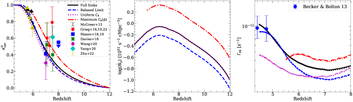
Figure 1: Volume-averaged ionized fraction (left), co-moving total ionizing emissivity (middle), and average photo-ionization rate in fully ionized cells (right) for each sinks model. All results shown here adopt our fiducial source scenario. We include measurements from the literature in the left panel (McGreer et al., 2015; Greig et al., 2016, 2019; Davies et al., 2018; Mason et al., 2018; Mason et al., 2019; Wang et al., 2020; Yang et al., 2020; Greig et al., 2022; Zhu et al., 2022). All the reionization histories are similar except the Maximum $\text{C}_{\text{R}}(\Delta)$ case. In the ensuing discussion, we show that the Full Sinks and Uniform $\text{C}_{\text{R}}$ models have nearly indistinguishable morphologies assuming our fiducial source model. Notably, although these models have the same reionization and emissivity histories, they have significantly different photo-ionization rates. Hence they may be distinguishable by observables that are sensitive to $\Gamma_{\rm HI}$, e.g. the mean free path and the Ly$\alpha$ forest.

In this section, we discuss the effect of sinks on the morphology of reionization. We compare our new sinks model to several representative alternatives. We assume our fiducial source model throughout (in §4 we will explore others.) We compare the following sink prescriptions:

• Full Sinks: Our fiducial sinks model is based on the suite of RadHydro simulations as described in § 2.2. The evolution of $\overline{\lambda}$ in each cell includes the dynamical effects of pressure smoothing and photoevaporation, as well as the impact of sub-resolved self-shielding on the IGM opacity.

• Relaxed Limit: For this model, we extrapolate the low-redshift $\overline{\lambda}$ from our $z_{\rm reion}=12$ RadHydro simulations to higher redshifts, assuming a power law in cosmic time, and directly interpolate $\overline{\lambda}$ instead of using Eq. 3. Thus, the gas is treated in the limit that it was ionized long ago and has reached a pressure-smoothed equilibrium. This model effectively removes the contribution of opacity from the initial clumpiness that is eventually erased during the relaxation process.

• Sub-grid Clumping Factor: Here we assume that all gas in ionized regions is in photo-ionization equilibrium at a constant $T=T_{\rm ref}\equiv 10^{4}$ K, which yields

  $$\overline{\lambda}=\frac{\Gamma_{\rm HI}}{\overline{\sigma}_{\rm HI}C_{\rm R}\alpha_{\rm B}(T_{\rm ref})(1+\chi)n_{\rm H}^{2}}$$ (4)

  where $\alpha_{\rm B}$ is the case B recombination coefficient of ionized hydrogen. We adopt two prescriptions for $C_{\rm R}$:

  1. Uniform $\text{\bf C}_{\text{\bf R}}$ : We set $C_{\rm R}=5$ everywhere at all times, which reproduces a reionization history and photon budget similar to the Full Sinks model. This case serves as a basis for comparison to assess the importance of the dynamics and spatial in-homogeneity of the sinks predicted by the Full Sinks model. We emphasize that $C_{\rm R}$ is a sub-grid clumping factor, not a global one.

  2. Maximum $\text{\bf C}_{\text{\bf R}}({\bm{\Delta}})$: We use the density-dependent sub-grid clumping factor of Mao et al. (2020). This model is based on dark-matter-only N-body simulations and predicts $C_{\rm R}\approx 10-15$ in cells with $\Delta\geq 1$ at $z\leq 8$. Since this model neglects pressure smoothing effects, it represents an upper limit on the amount of clumping in the standard cosmology.

The left-most panel in Figure 1 shows the volume-averaged ionized fraction for each sinks model alongside measurements from the literature. The middle panel shows the global ionizing emissivity. The emissivity histories are all re-scaled versions of the “rapid" model from Cain et al. (2021). For comparison, the emissivities of the Full Sinks, Relaxed Limit, and Uniform $\text{C}_{\text{R}}$ models have been tuned to yield very similar reionization histories and ionizing photon budgets, ending reionization late at $z=5-5.5$. The Maximum $\text{C}_{\text{R}}(\Delta)$ emissivity was tuned to end reionization somewhat earlier because the clumping factor fits from Mao et al. (2020) do not extend below $z\sim 6.5$. However, the ensuing morphology comparisons will be performed at fixed global ionized fraction, which should minimize any differences originating from the different reionization histories. Note that the Full Sinks and Uniform $\text{C}_{\text{R}}$ models have the same emissivity, while the Relaxed Limit (Maximum $\text{C}_{\text{R}}(\Delta)$) emissivity is a factor of $0.7$ ($2.4$) smaller (larger) than the other two. We note that due to the over-counting issue discussed in §2.3, the emissivity in the Full Sinks and Uniform $\text{C}_{\text{R}}$ models are likely higher than they should be. A lower photon budget would mean a smaller $C_{\rm R}$ in the latter to match the Full Sinks case; thus the value of $C_{\rm R}=5$ is probably too high. In the ensuing discussion we will see that our main conclusions on morphology are not significantly affected by this issue.

The right-most panel of Figure 1 shows $\Gamma_{\rm HI}$ averaged over fully ionized cells for each model, compared to measurements from Becker & Bolton (2013). Here we omit $z>5$ measurements (e.g. Calverley et al., 2011; Wyithe & Bolton, 2011; D’Aloisio et al., 2018; Becker et al., 2021) for clarity, and also because it is unclear how to compare these measurements against our $\Gamma_{\rm HI}$ in simulations where reionization is still ongoing at $z=5-6$. A number of reionization observables are explicitly sensitive to $\Gamma_{\rm HI}$, including the mean free path, Ly$\alpha$ forest statistics, and LAE visibility. In the ensuing discussion we will show that the Full Sinks and Uniform $\text{C}_{\text{R}}$ models exhibit essentially identical morphologies in our fiducial source model. A key takeaway from Figure 1 is that sink models tuned to yield similar morphologies, e.g. the Full Sinks and Uniform $\text{C}_{\text{R}}$ models, may nonetheless exhibit considerable differences in observables that are sensitive to $\Gamma_{\rm HI}$. So while these models may appear nearly identical in their predictions for the 21cm power spectrum, they will yield different predictions for e.g. Ly$\alpha$ forest statistics.

3.2 Visualization of the IGM Opacity

To aid in visualizing the dynamics and spatial morphology of the sinks, we define the “effective clumping factor” for cell $i$ to be

$$C_{\rm eff}^{i}=\frac{(1/\overline{\lambda}^{i})}{\overline{\sigma}_{\rm HI}\alpha_{B}(T_{\rm ref})(1+\chi){n_{\rm H}^{i}}^{2}/\Gamma_{\rm HI}^{i}},$$ (5)

where $T_{\rm ref}=10^{4}$ K and $\Gamma_{\rm HI}^{i}$, $\overline{\lambda}^{i}$, and $n_{\rm H}^{i}$ are the photo-ionization rate, mean free path, and H number density, respectively. The numerator is simply the absorption coefficient $\kappa$, and the denominator is what $\kappa$ would be if the gas had a constant temperature $T_{\rm ref}$, was in photo-ionizational equilibrium, and had no sub-resolved density fluctuations. $C_{\rm eff}$ quantifies the impact of sub-grid sink physics and large-scale temperature fluctuations on the opacity. In the limit of photo-ionizational equilibrium, Eq. 5 is equivalent to the recombination clumping factor $C_{R}$ (see § 2.3). Differences between $C_{\rm eff}$ and $C_{R}$ indicate the presence of sub-resolved self-shielded systems that are not in photo-ionizational equilibrium. Note that unlike in D’Aloisio et al. (2020), the density in the denominator of our clumping factors is the cell-wise density rather than the cosmic mean density. Thus, density fluctuations influence $C_{\rm eff}$ only indirectly through their impact on the sub-resolved clumpiness of the gas and its self-shielding properties.

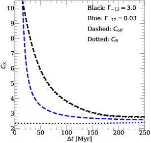
Figure 2: Examples of $C_{\rm eff}$ (dashed) compared to $C_{R}$ (dotted) for small-volume simulations with high and low values of $\Gamma_{-12}$ ($3.0$ and $0.03$). In the former, the two quantities are similar owing to the scarcity of self-shielded gas. However for $\Gamma_{-12}=0.03$, systems remain self-shielded and out of equilibrium for longer, producing a large difference between $C_{\rm eff}$ and $C_{R}$ since the former reflects the total number of absorptions but the latter only those balanced by recombinations.

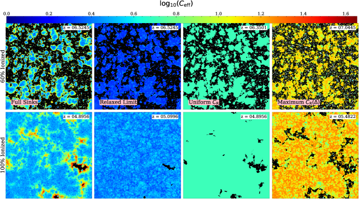
Figure 3: Visualization of the sink physics in each of our models. The redshifts are notated in the upper right of each panel. We show $\log_{10}(C_{\rm eff})$ at 60% volume ionized fraction (top) and $50$ Myr after reionization ends ($x_{\rm ion}^{\rm V}<0.01$, bottom row). The black regions denote cells that are at least $50\%$ ($10\%$) neutral in the top (bottom) panels. In the Full Sinks case, the opacity is boosted near I-fronts (top) and in under-dense voids that have yet to relax after reionization ends (bottom). The large scale fluctuations in $C_{\rm eff}$ are weaker in the other models. In the Uniform $\text{C}_{\text{R}}$ case, $C_{\rm eff}$ is the same everywhere, and in the Maximum $\text{C}_{\text{R}}(\Delta)$ models, $C_{\rm eff}$ is lower (higher) than average in voids (over-densities) after reionization, in contrast to the Full Sinks case. These visualizations illustrate the dynamical effects of pressure smoothing and photoevaporation in our Full Sinks model.

For intuition on $C_{\rm eff}$, Figure 2 shows its evolution (dashed curves) compared to that of $C_{R}$ (dotted curves) vs. time since ionization for two of our mean density, $z_{\rm reion}=8$ small-volume RadHydro simulations. One has $\Gamma_{-12}=3.0$ (black), and the other $0.03$ (blue). In the first case, $C_{\rm eff}$ and $C_{R}$ are close together; both start above $10$ and approach $\sim 3$ as the gas relaxes. Their similarity owes to the high intensity of the background, which leaves little gas self-shielded. In the $\Gamma_{-12}=0.03$ case, there is significant self-shielding in high-density gas. This lowers $C_{R}$ (which counts only recombination-balanced absorptions), while $C_{\rm eff}$ remains elevated, since it is affected by non-equilibrium absorptions taking place as the self-shielded gas is ionized. At later times, $C_{\rm eff}$ and $C_{R}$ agree better as more self-shielded systems evaporate.

Figure 3 shows slices of $\log(C_{\rm eff})$ from large-volume simulations for each of our sinks models (assuming our fiducial source model). We show the Full Sinks (left-most), Relaxed Limit (middle left), Uniform $\text{C}_{\text{R}}$ (middle right) and Maximum $\text{C}_{\text{R}}(\Delta)$ (right-most) models at $60$% volume ionized in the top row, and $50$ Myr after reionization has finished ($x_{\rm ion}^{\rm V}=0.01$) in the bottom row. The redshifts are given in the upper right of each panel. In the top (bottom) row, black regions denote cells that are at least $50\%$ ($10\%$) neutral (note that a small number of cells are still partially neutral even after $x_{\rm ion}^{\rm V}<0.01$ in the bottom row). In the Full Sinks model, $C_{\rm eff}$ is highest near I-fronts where gas was most recently ionized. After reionization ends, patches of enhanced opacity with $C_{\rm eff}\sim 10-20$ (and even higher in the most recently ionized cells) persist in the voids, which ionized last and quickly, so have yet to relax. In regions re-ionized earlier, $C_{\rm eff}$ is $\sim 2-5$ at all redshifts, similar to the Relaxed Limit. The opacity is higher in the Uniform $\text{C}_{\text{R}}$ case than in the Relaxed Limit because it has been calibrated to match the photon budget of the Full Sinks model. The Maximum $\text{C}_{\text{R}}(\Delta)$ model has the highest opacity, with $C_{\rm eff}\sim 10-20$ everywhere after reionization.

A comparison between the top-left and the two top-right panels in Fig. 3 reveals that the opacity in over-dense regions hosting the earliest ionized bubbles is significantly lower in our Full Sinks model compared to the Uniform $\text{C}_{\text{R}}$ and Maximum $\text{C}_{\text{R}}(\Delta)$ models. This results from the dynamics in our Full Sinks model, and may arise from two effects working in tandem: (1) $\Gamma_{\rm HI}$ is generally larger near the highly clustered sources, which leads to a quicker relaxation/evaporation of the sinks nearby ; (2) The structures that form in these regions may have a shorter relaxation time owing to their larger densities (see e.g. Eq. 4 of D’Aloisio et al., 2020). Together, these effects in our Full Sinks model work towards favoring the growth of larger bubbles compared to the Uniform $\text{C}_{\text{R}}$ and Maximum $\text{C}_{\text{R}}(\Delta)$ models. Conversely, the opacity is elevated in recently ionized regions at lower redshifts near the end of reionization, despite these regions being under-dense on average.

In the other three models, $C_{\rm eff}$ is affected mainly by density fluctuations, which are most noticeable in the Maximum $\text{C}_{\text{R}}(\Delta)$ model (and absent by construction in the Uniform $\text{C}_{\text{R}}$ case). In the Uniform $\text{C}_{\text{R}}$ model all parts of the IGM have the same $C_{\rm R}$, while in the Maximum $\text{C}_{\text{R}}(\Delta)$ model the over(under) dense regions have the highest (lowest) $C_{\rm R}$, opposite the Full Sinks case. We emphasize that the contrasting $C_{\rm eff}$ topologies will affect any observables that are explicitly sensitive to $\Gamma_{\rm HI}$ and the opacity structure of the IGM, such as the Ly$\alpha$ forest and the mean free path (see discussion of Fig. 1). However, in the ensuing discussion we will see that they are probably not very important for morphology.

3.3 Ionized Bubbles

3.3.1 Visualization of Ionized Region Morphology

Figure 4 shows the ionization field (darker = more neutral) for each of our sinks models (top to bottom, see labels) at 20, 50, and 80% volume ionized fraction (left to right). At fixed ionized fraction, the Maximum $\text{C}_{\text{R}}(\Delta)$ model exhibits the smallest ionized bubbles. This is indicated by the red shading, which denote regions that are neutral in the Maximum $\text{C}_{\text{R}}(\Delta)$ (and Uniform $\text{C}_{\text{R}}$) model, but not the Full Sinks case. The other models are visually similar to the Full Sinks case - the Uniform $\text{C}_{\text{R}}$model having slight smaller bubbles and the Relaxed Limit model having slightly larger ones (as indicated by the cyan shading in that row). The largest bubbles are smaller in the Maximum $\text{C}_{\text{R}}(\Delta)$ model because the sources driving their growth are “taxed” disproportionately by recombinations compared to those in smaller bubbles (Furlanetto & Oh, 2005). Since large bubbles form in over-densities and start growing the earliest, their growth is slowed by recombinations sooner than their later-forming counterparts inhabiting lower densities. Thus the sinks act to reduce the average bubble size at fixed ionized fraction (as found by e.g. Furlanetto & Oh, 2005; McQuinn et al., 2007; Alvarez & Abel, 2012; Mao et al., 2020; Chen et al., 2022).

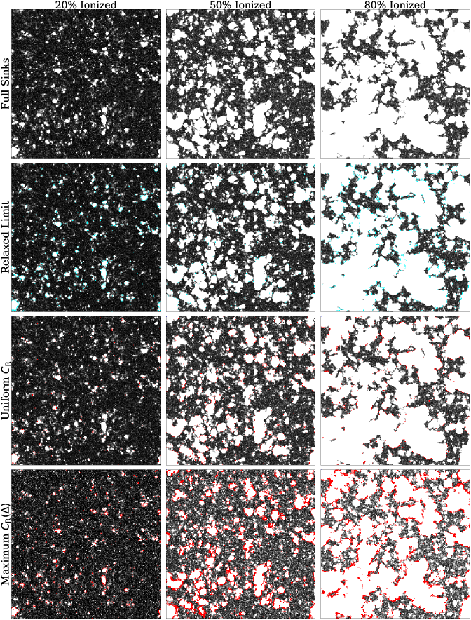
Figure 4: Visualization of the ionization field for our sinks models. All results here correspond to our fiducial source model with $\dot{n}_{\gamma}\propto L_{\rm UV}$, i.e. assuming the same escape fraction and ionizing efficiency for all sources. The columns show different volume ionized fractions ($20$, $50$, and $80$%, left to right) and the rows show different sinks models. In the second row, the cyan shading indicates bubbles that are slightly larger than in the Full Sinks model, while the red shading indicates the opposite in the other two rows. The ionized bubbles are smallest in the Maximum $\text{C}_{\text{R}}(\Delta)$ model at all ionized fractions. The Relaxed Limit model has slightly larger bubbles than the Full Sinks and Uniform $\text{C}_{\text{R}}$ models, but these three models are visually very similar.

Comparing the Full Sinks (top row) and Maximum $\text{C}_{\text{R}}(\Delta)$ (bottom row) models, the ionized bubbles generally appear larger in the former at fixed ionized fraction. As described in the previous section, this is a direct result of the dynamics in our sub-grid sinks model. In the earliest bubbles to form around highly clustered sources, the sinks relax/evaporate quickly, allowing the bubbles to grow more easily. By contrast, the smaller bubbles that start growing around less biased sources generally encounter a clumpier IGM for longer periods of time. Together, these effects work toward favoring the growth of large bubbles and partially cancel the “taxing the rich" effect described in the previous paragraph. The Maximum $\text{C}_{\text{R}}(\Delta)$ model instead has higher clumping factors at higher densities, which slows the growth of the largest bubbles more. In other words, our Full Sinks model taxes the rich less than the Maximum $\text{C}_{\text{R}}(\Delta)$ model, which does not include any dynamical effects.

Interestingly, in Figure 4 we see a striking degree of similarity between the Full Sinks and Uniform $\text{C}_{\text{R}}$ models at all ionized fractions. In fact, these models do not even differ significantly from the Relaxed Limit except near the beginning of reionization. The visual similarity leads us to one of our key conclusions, which we will hash out quantitatively in the ensuing sections. Accounting for the pressure-smoothing of the IGM by reionization is crucial for modeling morphology accurately. However, as long as this effect is accounted for “on average,” e.g. in the simplest case with a uniform sub-grid clumping factor, the detailed dynamics and spatial in-homogeneity of the sinks are likely not very important for morphology. We emphasize, however, that this conclusion holds only for source models in which bright galaxies contribute significantly to the ionizing photon budget, as in our fiducial source model. In §4, we will see scenarios for which the details of the sink modeling do become quite important.

3.3.2 Bubble Size Distribution

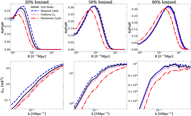
Figure 5: Top: Ionized Bubble Size Distribution (IBSD) for our sinks models (see legend) at 20%, 50%, and 80% volume ionized fractions (left to right). The Full Sinks and Uniform $\text{C}_{\text{R}}$ models have strikingly similar IBSDs despite their very different clumping topologies. Bottom: 21 cm power ($\Delta_{\rm 21}$) vs. wavenumber for the same models and ionized fractions. At $20\%$ ionized, the Maximum $\text{C}_{\text{R}}(\Delta)$ model is well below the Relaxed Limit, with the other two models in between, but closer to the Maximum $\text{C}_{\text{R}}(\Delta)$ result. At later times, the Full Sinks and Uniform $\text{C}_{\text{R}}$ models (which are always very similar to each other) move close to the Relaxed Limit. All results shown here adopt our fiducial source model with $\dot{n}_{\gamma}\propto L_{\rm UV}$.

Next, we study morphology more quantitatively using the ionized bubble size distribution (IBSD). We compute the IBSD using the ray-tracing definition proposed in Mesinger & Furlanetto (2007) and implemented in the publicly available package tools21cm (Giri et al., 2018). The IBSD defined this way captures the distribution of distances to neutral gas along random rays starting in ionized regions, and thus quantifies bubble sizes well even after ionized regions overlap. To exclude un-resolved bubbles from the BSD, we do not count a cell as part of an ionized bubble unless it is $\geq 99\%$ ionized. We caution that our simulations likely have too few resolved small bubbles - those with sizes $\sim$ a few $h^{-1}$Mpc - both due to our limited spatial resolution and our implementation of sub-resolved sources (see §2.4).

Figure 5 (top row) shows the IBSD at 20%, 50%, and 80% (left to right) for our sinks models. The IBSD confirms that the Maximum $\text{C}_{\text{R}}(\Delta)$ has the smallest bubbles at all times, and that the other three models have similar bubble sizes. The average bubble size is given at 20%, 50%, and 80% ionized for each model in Table 1. The mean values are mainly intended to illustrate the relative differences between our models. At $20\%$ and $50\%$ ionized the Relaxed Limit model has slightly larger bubbles, but at $80\%$ ionized is indistinguishable from the Full Sinks model. The bubble sizes for the Uniform $\text{C}_{\text{R}}$ model are slightly smaller than for the Full Sinks model, but are within $10-15\%$ at all times. We see from the Relaxed Limit comparison that even assuming a fully pressure-smoothed IGM at all times is a reasonable approximation for morphology, especially late in reionization.

Mean Bubble Size [$h^{-1}$Mpc]	20%	50%	80%
Full Sinks	1.94	7.30	30.08
Relaxed Limit	2.45	8.10	29.26
Uniform $\text{C}_{\text{R}}$	1.66	6.84	26.86
Maximum $\text{C}_{\text{R}}(\Delta)$	1.21	4.41	18.18

Table 1: Mean ionized bubble size at 20%, 50%, and 80% ionized for each of the sinks models in this section.

3.4 21 cm Power Spectrum

The 21 cm power spectrum, which probes the H i fluctuations in the IGM, is being targeted by PAPER (Parsons et al., 2010), MWA (Tingay et al., 2013), LOFAR (Yatawatta et al., 2013), HERA (DeBoer et al., 2017; Abdurashidova et al., 2022b, a), and forthcoming experiments such as SKA (Koopmans et al., 2015). Ignoring redshift-space distortions and assuming the spin temperature of the 21 cm transition $T_{S}$ is much greater than the CMB temperature, we can write the 21 cm brightness temperature at position $\vec{x}$ as

$$T_{21}(\vec{x})=\overline{T_{21}}x_{\rm HI}(\vec{x})(1+\delta(\vec{x}))$$ (6)

where $\overline{T_{21}}$ is $T_{21}$ at mean density in neutral gas, which depends on redshift and cosmology only, $x_{\rm HI}$ is the H i fraction, and $1+\delta$ is the gas density. The dimensionless 21 cm power spectrum is $\Delta_{21}\equiv k^{3}/2\pi^{2}P_{21}(k)$, where $P_{21}(k)$ is the power spectrum of $T_{21}$. Since $\Delta_{21}$ depends on $x_{\rm HI}$, it is sensitive to the differences in morphology between our sinks models.

Figure 5 (bottom row) shows $\Delta_{21}$ vs. wavenumber $k$ for our sinks models at 20%, 50%, and 80% ionized fractions (left to right). In all cases we see familiar qualitative features. Early on, $\Delta_{21}$ is steep in $k$ and its amplitude on large scales reaches a local minimum - a result of inside-out reionization (McQuinn & D’Aloisio, 2018; Giri et al., 2019b). Later, $\Delta_{21}$ flattens out and its amplitude at $k\leq 0.2$ $h^{-1}$Mpc has increased by $1-2$ orders of magnitude by an ionized fraction of 80%. (Note the different y axes on different panels.) This happens because the ionization field, which fluctuates on scales characteristic of the largest ionized bubbles ($10-30$ $h^{-1}$Mpc), takes over for the density field as the main driver of $\Delta_{21}$ at small $k$. Note that in this and in subsequent sections, we only show $\Delta_{21}$ for $k\leq 0.6$ $h$Mpc^-1, due to the caveat regarding the effects of sub-resolved halos discussed in §2.4.

The main effect of sinks is to reduce $\Delta_{21}$ on large scales ($k\leq 0.6$ hMpc^-1) by decreasing the sizes of large ionized bubbles. At $20\%$ ionized, $\Delta_{21}$ at $k=0.1h\text{Mpc}^{-1}$ for the (Relaxed Limit, Maximum $\text{C}_{\text{R}}(\Delta)$) model is ($1.75$, $0.59$) times its Full Sinks model value. At $50\%$ ionized these numbers become ($1.16$, $0.43$), and at $80\%$ ionized, they are ($1.0$, $0.69$). In all panels the Full Sinks and Uniform $\text{C}_{\text{R}}$ models are always within a few percent of each other. We see that the Maximum $\text{C}_{\text{R}}(\Delta)$ model, which neglects the effects of pressure smoothing, under-estimates the large-scale $\Delta_{21}$ by $\approx 30-60\%$ relative to the Full Sinks case during much of reionization. The Relaxed Limit over-estimates the power substantially only at $20\%$ ionized, and becomes an increasingly better approximation as reionization progresses.

The Maximum $\text{C}_{\text{R}}(\Delta)$ model illustrates that neglecting pressure smoothing can lead to a significant under-estimate of the large-scale power, owing to that model’s smaller ionized bubbles. On the other hand, assuming a fully relaxed IGM likely over-estimates the power early on, but becomes a reasonable approximation in the last half of reionization. Finally the similarity of the Full Sinks and Uniform $\text{C}_{\text{R}}$ models suggests that $\Delta_{21}$ is unlikely to be sensitive to the details of how sinks are modeled, as long as the dynamics of the sinks can be accounted for in an average fashion via a uniform sub-grid clumping factor. We caution, however, that all of these conclusions are sensitive to the properties of the sources, and we have employed only our fiducial source model so far. As we will see in §4.2, the impact of sinks becomes larger (smaller) when fainter (brighter) sources dominate the photon budget.

3.5 Neutral Islands

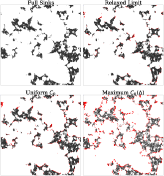
Figure 6: Visualization of neutral islands at 10% volume neutral fraction for our sinks models, assuming our fiducial source scenario. To aid comparison, the red shading highlights neutral regions that are ionized in the Full Sinks model. The Full Sinks, Relaxed Limit and Uniform $\text{C}_{\text{R}}$ models have visually similar island morphologies, while the Maximum $\text{C}_{\text{R}}(\Delta)$  case has more extended and more fragmented islands.

So far our focus has been the morphology of ionized bubbles during the bulk of reionization. However, a lot of progress toward understanding reionization is being made with the growing number of $z>5$ QSO absorption spectra, which may be probing the final phases of reionization when the mostly ionized IGM was punctuated by islands of neutral gas. Here we will briefly explore the morphology of these “neutral islands”. Neutral islands have been the focus of a number of recent studies (e.g. Xu et al., 2014; Malloy & Lidz, 2015; Xu et al., 2017; Giri et al., 2019a; Wu et al., 2022) owing to their importance for late-reionization observables.

In Figure 6, we illustrate the distribution of neutral gas at 10% volume neutral fraction using slices through our simulations. The red shading in each panel corresponds to neutral regions that are ionized in the Full Sinks model, i.e. to highlight differences in the neutral island morphology with that model. We see that the neutral islands in the Relaxed Limit and Uniform $\text{C}_{\text{R}}$ models differ very little from the Full Sinks case, while there are substantial differences with the Maximum $\text{C}_{\text{R}}(\Delta)$ model. In that model the neutral structures are more extended – as illustrated in red – but also appear to be a lighter shading of gray. This lighter shading indicates that the neutral islands are more porous, i.e. they contain a larger number of small ionized bubbles inside of them.

We quantify the morphology with the neutral island size distribution (NISD), defined analogously to the IBSD. Late in reionization, the NISD is sensitive to the definition of a “neutral” cell, since most of the cells with neutral gas are partially ionized, especially in models with high opacity. We define a cell to be part of an island if $x_{\rm HI}>0.01$. This choice is motivated by the fact that a sightline intersecting a partially neutral cell must pass within $1$ Mpc/h of an ionization front. Gas this close to I-fronts typically has a low photo-ionization rate (Nasir & D’Aloisio, 2020) and/or is un-relaxed (Park et al., 2016; D’Aloisio et al., 2020) and is thus likely to be opaque to both LyC and Ly$\alpha$ photons.

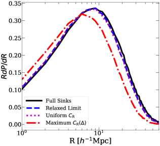
Figure 7: Neutral island size distribution defined such that any cell with $x_{\rm HI}>0.01$ is part of an island. We include all the sinks models in Figure 5 and adopt our fiducial source model. The Maximum $\text{C}_{\text{R}}(\Delta)$ model has smaller islands, while the NISDs for the other three models are all very similar.

Figure 7 shows the NISD at 10% volume neutral fraction for our sinks models (which occurs at $z\approx 5.5$ for all models except the Maximum $\text{C}_{\text{R}}(\Delta)$ case, which is shown at $z\approx 6.0$). The Maximum $\text{C}_{\text{R}}(\Delta)$ model has the smallest islands while the other models are all very similar. The average island sizes for the Relaxed Limit, Full Sinks, Uniform $\text{C}_{\text{R}}$ and Maximum $\text{C}_{\text{R}}(\Delta)$ models are $7.5$ $h^{-1}$Mpc, $7.9$ $h^{-1}$Mpc, $7.4$ $h^{-1}$Mpc, and $5.8$ $h^{-1}$Mpc, respectively. In spite of the Maximum $\text{C}_{\text{R}}(\Delta)$ model having more spatially extended neutral structures, the large abundance of small ionized bubbles within these structures break them up and shift the NISD towards smaller sizes. We see that even the approximation of a fully pressure-smoothed IGM is likely acceptable for capturing the morphology of neutral islands. On the other hand, ignoring pressure smoothing effects leads to a $\approx 20\%$ under-estimate of the mean island size in our fiducial source model.

4 Interplay Between Sources and Sinks

4.1 Source Models

Figure 8: Ionization maps at 50% volume ionized for the Democratic Sources (left), Fiducial (middle) and Oligarchic Sources (right) models, all assuming the Full Sinks model. From left to right, the contribution to the photon budget from the brightest, most massive halos increases. Reionization by more massive, highly biased sources leads to ionized bubbles being larger and fewer in number.

In this section, we will generalize our analysis to include different models for the sources. Most previous studies of morphology have varied the source and sinks properties one at a time, while keeping the other fixed (e.g. McQuinn et al., 2007; Shukla et al., 2016; Mao et al., 2020; Giri et al., 2019a; Wu et al., 2022; Chen et al., 2022). Our use of efficient RT simulations with sink dynamics included allows us to explore the relationship between the sources and sinks as it pertains to morphology. We consider three models for the sources:

• Democratic Sources: This model differs from our fiducial model in that it assigns all halos the same ionizing emissivity independent of their luminosity, i.e. $\beta=0$ (see §2.4). At $z=6$, 50% of the ionizing emissivity is produced by halos in the mass range $10^{9}<M/[{\rm h}^{-1}M_{\odot}]<1.8\times 10^{9}$ ($-12.6>M_{\rm UV}>-13.4$). This model was introduced in Cain et al. (2021) in an attempt to find a model that better recovers the short mean free path at $z=6$ reported by Becker et al. (2021). This kind of picture would require a steep dependence of $f_{\rm esc}$ and/or the ionizing efficiency $\xi_{\rm ion}$ on luminosity, specifically, $f_{\rm esc}\xi_{\rm ion}\propto L_{\rm UV}^{-1}$ (corresponding to roughly $f_{\rm esc}\xi_{\rm ion}\propto M^{-1.4}$ over most of the mass range at $z=6$). The sources driving reionization in this model are almost entirely below current detection limits, in contrast to the Oligarchic Sources model described below.

• Fiducial Sources: Our fiducial scenario with $M_{\min}=10^{9}$ $h^{-1}M_{\odot}$ and with the emissivity of each halo proportional to its UV luminosity (i.e. $\beta=1$). At $z=6$, halos with masses in the range $10^{9}<M/[{\rm h}^{-1}M_{\odot}]<1.8\times 10^{10}$ ($-12.6<M_{\rm UV}<-16.9$) contribute $50\%$ of the ionizing emissivity. Of our three source models, this one is most similar to parameterizations commonly used in simulations, e.g. those that assume the emissivity to be proportional to halo mass (Mao et al., 2020; Keating et al., 2020a, b; Bianco et al., 2021).

• Oligarchic Sources: In this model, bright and massive sources – the “oligarchs” – dominate reionization. We adopt $M_{\min}=2\times 10^{10}$ $h^{-1}M_{\odot}$ with $\beta=1$, corresponding to a limiting magnitude of $M^{\max}_{\rm UV}(z=6)\approx-17$, roughly the limit of current observations at $5<z<10$ (Finkelstein, 2016; Bouwens et al., 2021). Thus it assumes that the sources responsible for reionization have, for the most part, already been observed. This model is qualitatively similar to that proposed by Naidu et al. (2020) (see also Naidu et al. (2022); Matthee et al. (2022)). It also serves to contrast starkly with the Democratic Sources model.

To make some contact with previous works exploring how the source properties affect morphology, Figure 8 shows ionization maps at 50% volume ionized ($z\sim 7$) for our Democratic Sources (left), Fiducial Sources (middle) and Oligarchic Sources (right), all assuming the Full Sinks model. The differences are clearly visible in the ionization fields; in the models driven by brighter sources, the ionized bubbles are larger and fewer in number. This is because the most massive, rare sources produce a larger fraction of the photons in the Fiducial and Oligarchic Sources models. This familiar result has been observed in many previous studies (e.g. McQuinn et al., 2007; Giri et al., 2019a; Kannan et al., 2022; Chen et al., 2022). Now we turn our attention to the interplay between the sources and sinks.

4.2 Results

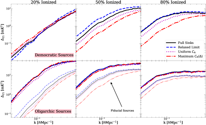
Figure 9: $\Delta_{21}(k)$ for all our sources and sinks models, illustrating the interplay between the sources and sinks of reionization. The top and bottom rows show results for the Democratic Sources and Oligarchic Sources models, respectively. The Fiducial Sources result is shown again by the thin curves in the bottom panel for comparison. The magnitude of the sinks’ effect on morphology clearly depends on the nature of the sources. In the Democratic Sources scenario (top row), the differences between the sinks models are significantly larger than in the Oligarchic Sources scenario. Notably, in the former, the Uniform $\text{C}_{\text{R}}$ model no longer matches so well the Full Sinks results, as it did for Fiducial Sources (compare to the thin curves in the bottom row). By contrast, in the Oligarchic Sources scenario, even the Maximum $\text{C}_{\text{R}}(\Delta)$ model matches the others well, especially at 50% and 80% ionization. We are led to conclude that in reionization scenarios driven by less (more) biased sources, the sinks become more (less) important for shaping morphology.

Figure 9 shows $\Delta_{21}(k)$ at 20%, 50%, and 80% ionized, in the same format as the bottom panel of Figure 5, for all combinations of source and sinks models. The top and bottom rows show results for the Democratic Sources and Oligarchic Sources models, while the results for the Fiducial Sources model (same as Figure 5) are shown by the thin lines in the bottom row. Note that models sharing the same sinks prescription have similar reionization histories and the same emissivity histories as those shown in Fig. 1. In the Democratic Sources case, the differences between sinks models are smaller at $20\%$ ionized but somewhat larger at $50\%$ and $80\%$ ionized than in the Fiducial Sources case. The suppression of $\Delta_{21}$ at $k=0.1$ $h$Mpc^-1 in the latter half of reionization relative to the Full Sinks case has increased from $30-60\%$ for the Fiducial Sources case to $70-80\%$. In addition, there are now $\approx 40\%$ differences between the Relaxed Limit, Full Sinks, and Uniform $\text{C}_{\text{R}}$ models at $50\%$ ionized. The Uniform $\text{C}_{\text{R}}$ model is $\approx 35\%$ below the Full Sinks and Relaxed Limit models at $80\%$ ionized.

It is interesting that for the Democratic Sources model (top row) the Full Sinks and Uniform $\text{C}_{\text{R}}$ models have appreciably different $\Delta_{21}$. In particular, the Full Sinks model has more large-scale power, which is indicative of larger ionized bubbles. Recall from our discussion in §3.2 that the Full Sinks model should be expected to favor the growth of larger bubbles more than the Uniform $\text{C}_{\text{R}}$ case owing to lower (higher) clumping factors in over-dense (under-dense) regions in the former. It seems that the these differences, which had little effect on morphology in our Fiducial Sources model, do become important in the limit that very faint, low-bias sources drive reionization. We caution that this effect may be exaggerated due to our probable over-estimation of the impact of un-relaxed gas, discussed in §2.3. However, it may also be a slight under-estimate due to the effects of using sub-resolution sources, as discussed in §2.4. In our tests using the Democratic Sources + Uniform $\text{C}_{\text{R}}$  combination, fixing the positions of the sources (see last paragraph of §2.4) can reduce power at $k=0.1$ $h$Mpc^-1 by up to $20\%$, while the Full Sinks model does not change appreciably. This reduction in power was as large as a factor of $2$ in our tests using the Democratic Sources + Maximum $\text{C}_{\text{R}}(\Delta)$  combination. We note that these differences would work in the direction of strengthening our conclusions in these scenarios, and that for the other source models we found differences of $10\%$ or less.

By contrast, in the Oligarchic Sources case, the differences are $15\%$ or less between the Full Sinks, Relaxed Limit, and Uniform $\text{C}_{\text{R}}$ models in all of the panels. More strikingly, at $50\%$ and $80\%$ ionized even the Maximum $\text{C}_{\text{R}}(\Delta)$ model is very similar to the Uniform $\text{C}_{\text{R}}$ case. The insensitivity of morphology to the sinks in the Oligarchic Sources model contrasts the much stronger dependence seen in the Democratic Sources model.

Why is morphology sensitive to the sinks in models driven by fainter sources, but not in the Oligarchic Sources scenario? In §3, we saw that sinks limit the sizes of large ionized bubbles. However, it is harder for them to do so in the Oligarchic Sources scenario for two reasons. Nearly all the emissivity is concentrated in highly biased regions, strongly favoring the growth of the largest ionized bubbles. Second, these bubbles grow fast enough to escape the over-densities in which they are born before recombinations begin having a significant impact. This mitigates the “disadvantage” those bubbles have of inhabiting over-dense regions. In these ways, sources in the Oligarchic Sources model “win out” over the sinks in terms of shaping morphology. In the Democratic Sources model, by contrast, the sources are less biased than in Fiducial Sources and the sinks can more easily slow the growth of the largest bubbles. In other words, the sinks are unable to tax the rich enough to affect morphology when the source bias is very high, and become more effective at taxing them when the source bias is reduced.

This result has implications for forthcoming efforts to model reionization and interpret observations. Most straightforwardly, it demonstrates that studying the sinks and sources one at a time can produce biased results. For example, studying the sinks in a scenario with only highly biased sources would lead to the incorrect conclusion that they are unimportant for morphology. Another point is that very highly-biased source models may be relatively easy to rule out (or confirm) with forthcoming 21 cm observations from reionization. For example, an upper limit of e.g. $\Delta_{21}(k=0.1\text{ hMpc}^{-1})\leq 10$ mK² midway through reionization would strongly disfavor the Oligarchic Sources model (which has $\Delta_{21}(k=0.1\text{ hMpc}^{-1})\approx 20$ mK² at $x_{\rm ion}^{\rm V}=0.5$), since any physically reasonable sinks model would be unable to push $\Delta_{21}$ much lower than this. The tightest upper limit to date from HERA (Abdurashidova et al., 2022b) is $\Delta_{21}\leq 946$ mK² at $z\sim 7.9$ and $k=0.19$ $h$Mpc^-1, less than 2 dex away from reaching the prediction of our Oligarchic Sources model. Other probes that are sensitive to the existence of large ionized regions, such as the visbility of LAEs at $z>6$ (Vanzella et al., 2011; Jung et al., 2020; Tilvi et al., 2020; Endsley et al., 2021), may also be able to identify large bubbles like those predicted by the Oligarchic Sources model.

5 Conclusion

At present, there is no consensus on how much of an effect the sinks had in shaping reionization’s morphology and, relatedly, how important they are for interpreting its observables. We have attempted to address these questions using cosmological RT simulations of reionization. Our simulations include the sub-grid model for the ionizing photon opacity developed by Cain et al. (2021), which is based on high-resolution, fully coupled radiative hydrodynamics simulations of the IGM. The model improves over previous efforts in several key ways: it includes the effects of self-shielding and hydrodynamic response to photo-heating, keeping track of their dependencies on the LyC intensity, the timing of (local) reionization, and the environmental density. Our main conclusions can be summarized as follows:

• The sinks decrease the sizes of the largest ionized bubbles during reionization. We explored this effect in our detailed sub-grid model (Full Sinks), and in three other models representative of the ways that sinks have been implemented in previous studies: (1) A model that assumes a pressure-smoothed IGM (Relaxed Limit); (2) A simple clumping factor without dynamics or spatial in-homogeneity, tuned to have the same photon budget as our fiducial model (Uniform $\text{C}_{\text{R}}$); (3) An in-homogeneous clumping model from Mao et al. (2020) that neglects pressure smoothing, thus representing a kind of upper limit on the effects of sinks (Maximum $\text{C}_{\text{R}}(\Delta)$).

• For our fiducial source model, which assumes the same escape fraction and ionizing efficiency for all sources, the Full Sinks model has up to $\sim 10-20\%$ smaller mean bubble sizes compared to the Relaxed Limit model in the first half of reionization. These differences mostly disappear in the second half.

• By contrast, the Maximum $\text{C}_{\text{R}}(\Delta)$ model underestimates bubble sizes by $\approx 40\%$ (compared to the Full Sinks model). Ignoring the dynamical effects of pressure smoothing and photoevaporation can over-estimate significantly the sinks’ effects on morphology.

• We were able to reproduce a very similar morphology to our Full Sinks model using a uniform constant sub-grid clumping factor (the Uniform $\text{C}_{\text{R}}$ model). Hence, under typical assumptions about reionization’s source population, with regards to morphology, it appears that the detailed dynamics and spatial in-homogeneity of the sinks can be adequately modeled in an average sense with a sub-grid clumping factor. This is a useful result for scenarios where either (1) the ionizing photon budget is fixed by a model (as in this work) or by some empirical constraint, or (2) the budget is free to vary, as in a parameter space study. To apply this result to a reionization simulation, one may simply re-scale the recombination rates at $T_{\rm ref}=10,000$ K by a uniform sub-grid clumping factor, $C_{\rm R}$, tuned to match the given total ionizing photon budget. Note, however, that the Full Sinks and Uniform $\text{C}_{\text{R}}$ models exhibit significant differences in $\Gamma_{\rm HI}$ (Fig. 1), which could render predictions for, e.g., the Ly$\alpha$ forest quite different. As such, we emphasize that this conclusion should only be taken to apply to the structure of ionized and neutral regions, and not other physical properties of the ionized IGM, such as $\Gamma_{\rm HI}$ or the mean free path.

• Differences in bubbles sizes between our models are manifest in the predicted power spectrum of the red-shifted 21cm background. The Maximum $\text{C}_{\text{R}}(\Delta)$ under-estimates the large-scale 21 cm power by $30-60\%$ throughout reionization compared to our Full Sinks model for our fiducial source prescription. The Relaxed Limit model over-estimates power somewhat early in reionization, but becomes similar to both the Full Sinks and Uniform $\text{C}_{\text{R}}$ cases in reionization’s latter half.

• The morphology of neutral islands near the end of reionization is very similar in all of the models except the Maximum $\text{C}_{\text{R}}(\Delta)$ case, which produces smaller islands. The islands in that model are $20\%$ too small on average, highlighting again the importance of including the effects of pressure smoothing.

• The strength of the sinks’ effect on morphology is sensitive to the properties of the sources that drove reionization. In a model where reionization was driven entirely by bright ($M_{\rm UV}<-17$), highly biased galaxies, the sinks suppress the 21 cm power at the $10-15\%$ level at a fixed ionized fraction throughout reionization, even in the Maximum $\text{C}_{\text{R}}(\Delta)$ case. By contrast, when faint ($M_{\rm UV}\sim-13$), low-bias galaxies drove reionization, the large-scale 21 cm power can be suppressed by up to $80\%$, and the morphology in the Full Sinks and Uniform $\text{C}_{\text{R}}$ models differ significantly. This result highlights the need to study the effects of sinks and sources together instead of separately. Moreover, the insensitivity of morphology to sinks in highly biased source models makes such models easier targets for forthcoming 21 cm experiments like HERA and SKA, and other probes sensitive to the presence of very large ionized bubbles.

Our Full Sinks model can be improved on in several ways. First, in future iterations we plan to address the caveats discussed in §2.3, namely the possible under-counting of rare, massive sinks and double-counting of absorptions in self-shielded systems. These issues can be addressed with sub-grid simulations in larger volumes and by explicitly modeling the evolution of the residual H i fraction in self-shielded systems. A notable uncertainty in our results is that simulations upon which our sub-grid model is based do not include galaxy formation processes, which may affect significantly the structure and state of sinks near massive halos.

Given the interplay between sources and sinks pointed out here, future studies should also move beyond simplistic source parameterizations. Source models should ideally incorporate physically motivated prescriptions for effects such as feedback from reionization (Shapiro et al., 1994; Thoul & Weinberg, 1996; Gnedin, 2000; Hoeft et al., 2006; Finlator et al., 2011; Wu et al., 2019; Ocvirk et al., 2021), bursty star formation (Weisz et al., 2011; Emami et al., 2019; Furlanetto & Mirocha, 2022), galaxy formation histories (Bullock et al., 2000; Somerville & Davé, 2015; Mirocha et al., 2021), and for $f_{\rm esc}$ (Kuhlen & Faucher-Giguère, 2012; Barrow et al., 2020; Maji et al., 2022; Marques-Chaves et al., 2022; Yeh et al., 2022), all of which play important roles in setting the abundance and bias of the sources.

Data Availability

The data underlying this article will be shared upon reasonable request to the corresponding author.

Appendix A Numerical Convergence

Here we describe some additional parameters in our code and demonstrate convergence of the ionization field in our simulations. The first parameter is $N_{\rm iter}$, the number of times Eq. 1 is iterated with the equation for $\overline{\lambda}$ (Eq. 3 or 4) during each time step. Our fiducial value is $N_{\rm iter}=5$. Our initial guess for $\Gamma_{\rm HI}$ assumes $\overline{\lambda}>>\Delta x_{\rm cell}$, where $\Delta x_{\rm cell}$ is the cell size, in which limit Eq. 1 is independent of $\overline{\lambda}$. Thus in general, convergence takes longest when $\overline{\lambda}\lesssim\Delta x_{\rm cell}$ - that is, in optically thick cells. To test convergence of $N_{\rm iter}$, we ran simulations with $N_{\rm iter}=1$, $3$, $5$, and $10$ on a coarse-grained ($N=150^{3}$; $\Delta x_{\rm cell}=2~{}h^{-1}$Mpc) version of our reionization volume using the Democratic Sources and Maximum $\text{C}_{\text{R}}(\Delta)$ models. This is the most extreme combination of source and sinks scenarios since it has the shortest $\overline{\lambda}$ on average. In Fig. 10 we show $\Delta_{21}(k)$ vs. wavenumber at 30% and 70% ionized for our tests, re-scaled so that the two sets of curves can be distinguished. At $k=0.1$ $h$Mpc^-1, the $N_{\rm iter}=5$ and $10$ cases are $\approx 10\%$ apart at $30\%$ ionized and $35\%$ apart at $70\%$ ionized. This is considerably less than the factor of several difference between the Maximum $\text{C}_{\text{R}}(\Delta)$ and Full Sinks models the top row of Figure 9. We have checked convergence for different combinations of sinks and source models and found better convergence in all cases. Moreover, this result is conservative because the condition $\overline{\lambda}\lesssim\Delta x_{\rm cell}$ is more likely to occur for $\Delta x_{\rm cell}=2$ $h^{-1}$Mpc than for our fiducial $\Delta x_{\rm cell}=1$ $h^{-1}$Mpc.

Next we checked for convergence in the angular resolution of the radiation field. This is adjustable in our code through two parameters that control how rays are merged. The first, $l_{\rm hpx}$, is the order of the HealPix sphere onto which rays are binned when they are merged. Our fiducial $l_{\rm hpx}=0$ corresponds to keeping track of $12$ directions. The other parameter is $N_{\rm ex}$ - the number of rays per cell that are “exempt” from being merged. Before rays merged, they are sorted in order of their photon counts, and the top $N_{\rm ex}N^{3}$ rays are not considered for merging. Using the same coarse-grained setup, we checked all combinations of $l_{\rm hpx}=0$ and $1$ (which corresponds to tracking $48$ directions) and $N_{\rm ex}=16$ (our fiducial choice) and $44$. We found that $\Delta_{21}$ for these tests (not shown) to be indistinguishable for all combinations of these parameters on scales of interest, despite the amount of noise in the radiation field decreasing considerably for higher resolution runs.

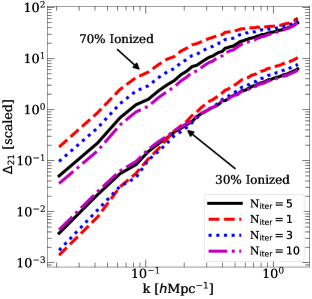
Figure 10: $\Delta_{21}(k)$ at 30% and 70% ionized (see annotations) for four values of $N_{\rm iter}$ (see legend). This test uses the Democratic Sources and Maximum $\text{C}_{\text{R}}(\Delta)$ models (the combination with the shortest $\overline{\lambda}$) in a coarse-grained version of the original simulation volume with $2$ $h^{-1}$Mpc cells. Our fiducial value of $N_{\rm iter}=5$ is within 10% or the $N_{\rm iter}=10$ case at $30\%$ ionized and within $35\%$ at $70\%$ ionized at all $k$. This is relatively small compared to the differences seen in the top row of Figure 9. Moreover, all the other combinations of models that we checked displayed significantly better convergence.

Appendix B Derivation of Eq. 1 (for $\Gamma_{\rm HI}$)

Here we will derive Eq. 1 for $\Gamma_{\rm HI}$. Consider cell $i$ with ionized fraction $x_{\rm ion}^{i}$ and volume $V_{\rm cell}$. If the I-front in cell $i$ is infinitely sharp and travels along one axis, then ray $j$ intersecting cell $i$ will travel a distance $x_{\rm ion}^{i}\Delta s^{ij}$ (recall $\Delta s^{ij}$ is the total path length of ray $j$ through cell $i$) before reaching neutral gas. The number of photons absorbed over this distance is

$$N_{\rm abs}^{i}=\sum_{j=1}^{N_{\rm rays}}N_{0}^{ij}\left(1-\exp\left[\frac{-x_{\rm ion}^{i}\Delta s^{ij}}{\overline{\lambda}^{i}}\right]\right)$$ (7)

where $N_{0}^{ij}$ is the number of photons in ray $j$ entering cell $i$ and $\overline{\lambda}$ is the mean free path in cell $i$ behind the I-front. During a time step $\Delta t$, $\Gamma_{\rm HI}$ behind the I-front is

$$\Gamma_{\rm HI}^{i}=\frac{\text{\# of photons absorbed per time}}{\text{\# of HI atoms in ionized gas}}=\frac{N_{\rm abs}^{i}/\Delta t}{n_{\rm HI}^{\Gamma}x_{\rm ion}^{i}V_{\rm cell}}$$ (8)

where $x_{\rm ion}^{i}V_{\rm cell}$ is the ionized volume of cell $i$ and

$$n_{\rm HI}^{\Gamma}\equiv\frac{\langle\Gamma_{\rm HI}n_{\rm HI}\rangle_{\rm V}}{\langle\Gamma_{\rm HI}\rangle_{\rm V}}$$ (9)

is the $\Gamma_{\rm HI}$-weighted HI number density (the V sub-script denotes a volume average). Eq. 2 relates the numerator of Eq. 9 to our definition for $\overline{\lambda}$ for the small-volume simulations (derived in the next section). Combining Eqs. 2, 9, and 7 yields

$$\Gamma_{\rm HI}^{i}=\sum_{j=1}^{N_{\rm rays}}\frac{N_{0}^{ij}\left(1-\exp\left[-x_{\rm ion}^{i}\Delta s^{ij}/\overline{\lambda}^{i}\right]\right)}{(\overline{\lambda}^{-1}F_{\gamma}/\langle\Gamma_{\rm HI}\rangle_{\rm V})x_{\rm ion}^{i}V_{\rm cell}\Delta t}$$ (10)

where $F_{\gamma}\equiv\Gamma_{\rm HI}^{0}\overline{\sigma}_{\rm HI}^{-1}$ is the ionizing flux at the source planes in the small-volume simulations and $\Gamma_{\rm HI}^{0}$ is the photo-ionization rate at the source planes. Because the domain size (32 $h^{-1}$kpc) is much less than $\overline{\lambda}$ in all our small-volume simulations, $F_{\gamma}$ usually attenuates very little over the domain width except around self-shielded systems, which (typically) occupy a small fraction of the volume. Thus, $\langle\Gamma_{\rm HI}\rangle_{\rm V}\approx\Gamma_{\rm HI}^{0}$, which gives

$$\Gamma_{\rm HI}^{i}\approx\sum_{j=1}^{N_{\rm rays}}\frac{N_{0}^{ij}\left(1-\exp\left[-x_{\rm ion}^{i}\Delta s^{ij}/\overline{\lambda}^{i}\right]\right)}{(\overline{\lambda}\overline{\sigma}_{\rm HI})^{-1}x_{\rm ion}^{i}V_{\rm cell}\Delta t}$$ (11)

which is equivalent to Eq. 1.

Note that Eq. 8 and Eq. 11 together imply that $n_{\rm HI}^{\Gamma}\approx(\overline{\lambda}\overline{\sigma}_{\rm HI})^{-1}$ should be true in our small-volume simulations. Figure 11 tests this equality for simulations with $\Gamma_{-12}=3.0$ (blue curves), $0.3$ (red) and $0.03$ (black) for $z_{\rm re}=8$ and $\delta/\sigma=0$ (mean density). The top panel plots both quantities vs. time since ionization, while the bottom panel shows their ratio. In the simulations with $\Gamma_{-12}=3.0$ and $0.3$ the equality holds to within a few percent even during the first few Myr when self-shielding is most important. However in the $0.03$ case, they do not agree to within 10% until $\approx 10$ Myr after ionization. In that case, $n_{\rm HI}^{\Gamma}>(\overline{\lambda}\overline{\sigma}_{\rm HI})^{-1}$, Eq. 1 under-estimates the number of absorptions in ionized gas because it over-estimates $\Gamma_{\rm HI}$, and therefore the converged value of $\overline{\lambda}$ (Eq. 3). This works in the direction of making the opacity too low in recently ionized gas with low $\Gamma_{\rm HI}$ in our reionization simulations. However, the double-counting issue described in §2.3 likely still renders the total opacity in these regions an over-estimate. The test and photon budget comparison described in that section includes the effect discussed here, so our statements there should still hold.

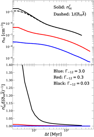
Figure 11: Test of the relation $n_{\rm HI}^{\Gamma}=(\overline{\lambda}\overline{\sigma}_{\rm HI})^{-1}$, as required by Eq. 1. Top: $n_{\rm HI}^{\Gamma}$ (solid) and $(\overline{\lambda}\overline{\sigma}_{\rm HI})^{-1}$ (dashed) vs. time since ionization for small-volume simulations with $\Gamma_{-12}=3.0$ (blue), $0.3$ (red), and $0.03$ (black), assuming $z_{\rm re}=8$ and $\delta/\sigma=0$. Bottom: the ratio between these two quantities for each case. For $\Gamma_{-12}=3.0$ and $0.3$ the equality holds within a few percent at all times, but for $0.03$ agreement to within 10% is not reached until $\Delta t\approx 10$ Myr. This works in the direction of under-estimating the absorption rate in recently ionized cells with low $\Gamma_{\rm HI}$ in our reionization simulations.

Appendix C Derivation of Eq.2 (for $\overline{\lambda}$)

In this section we derive our estimator for the frequency-averaged mean free path in our small-volume simulations, $\overline{\lambda}$ (Eq. 2). Let $I_{\nu}$ be the specific intensity at the source planes. The ionizing flux along one direction of our box is,

$$F_{\gamma}=\int^{4\nu_{\rm HI}}_{\nu_{\rm HI}}\frac{I_{\nu}}{h_{p}\nu}~{}d\nu,$$ (12)

where $h_{p}$ is Planck’s constant and $h_{p}\nu_{\rm HI}$ is the ionization potential of hydrogen. Assuming the radiation streams along the $x_{1}$ direction, the photoionization rate at location $\mathbf{x}=(x_{1},x_{2},x_{3})$ along a ray is

$$\Gamma_{\rm HI}(\mathbf{x})=\int^{4\nu_{\rm HI}}_{\nu_{\rm HI}}\frac{\sigma_{\nu}}{h\nu}I_{\nu}e^{-\int^{x_{1}}_{0}dx^{\prime}n_{\rm HI}(x^{\prime},x_{2},x_{3})\sigma_{\nu}}~{}d\nu,$$ (13)

where $n_{\rm HI}(\mathbf{x})$ is the proper hydrogen number density and $\sigma_{\nu}$ is its photoionization cross section. We can write

$$n_{\rm HI}(\mathbf{x})~{}\Gamma_{\rm HI}(\mathbf{x})=\int^{4\nu_{\rm HI}}_{\nu_{\rm HI}}d\nu\frac{I_{\nu}}{h\nu}~{}n_{\rm HI}(\mathbf{x})\sigma_{\nu}~{}e^{-\int^{x_{1}}_{0}dx^{\prime}n_{\rm HI}(x^{\prime},x_{2},x_{3})\sigma_{\nu}}=$$

$$-\int^{4\nu_{\rm HI}}_{\nu_{\rm HI}}d\nu\frac{I_{\nu}}{h\nu}\frac{\partial}{\partial x_{1}}e^{-\int^{x_{1}}_{0}dx^{\prime}n_{\rm HI}(x^{\prime},x_{2},x_{3})\sigma_{\nu}}$$ (14)

Integrating over the domain volume $V_{d}=L_{d}^{3}$, we obtain

$$V_{d}\langle n_{\rm HI}\Gamma_{\rm HI}\rangle_{V_{d}}=$$

$$\int^{4\nu_{\rm HI}}_{\nu_{\rm HI}}d\nu\frac{I_{\nu}}{h\nu}\int_{0}^{L_{d}}dx_{2}dx_{3}~{}\left(1-e^{-\int^{L_{d}}_{0}dx^{\prime}n_{\rm HI}(x^{\prime},x_{2},x_{3})\sigma_{\nu}}\right)$$ (15)

where $\langle\ldots\rangle_{V_{d}}$ denotes an average over the domain volume. We define the effective optical depth through

$$e^{-\tau_{\mathrm{eff}}}\equiv\langle e^{-\int^{L_{d}}_{0}dx^{\prime}n_{\rm HI}(x^{\prime},x_{2},x_{3})\sigma_{\nu}}\rangle_{A_{d}}=$$

$$A_{d}^{-1}\int_{0}^{L_{d}}dx_{2}dx_{3}~{}e^{-\int^{L_{d}}_{0}dx^{\prime}n_{\rm HI}(x^{\prime},x_{2},x_{3})\sigma_{\nu}}$$ (16)

where $A_{d}=L_{d}^{2}$ and $\langle\ldots\rangle_{A_{d}}$ denotes an average over the transverse plane. Plugging this into equation 15 yields

$$L_{d}\langle n_{\rm HI}\Gamma_{\rm HI}\rangle_{V_{d}}=\int^{4\nu_{\rm HI}}_{\nu_{\rm HI}}d\nu\frac{I_{\nu}}{h\nu}(1-e^{-\tau_{\mathrm{eff}}}).$$ (17)

The mean free path is defined to be $\overline{\lambda}=L_{d}/\tau_{\mathrm{eff}}$. Assuming that $\lambda\gg L_{d}$ (recall that $L_{d}=32h^{-1}$ kpc), we can expand the exponential in equation 17 to first order, yielding

$$\overline{\lambda}^{-1}\equiv\langle\lambda^{-1}\rangle_{\nu}=\frac{\langle n_{\rm HI}\Gamma_{\rm HI}\rangle_{V_{d}}}{F_{\gamma}},$$ (18)

where we have used that $\langle\lambda^{-1}\rangle_{\nu}=(1/F_{\gamma})\int^{4\nu_{\rm HI}}_{\nu_{\rm HI}}d\nu\frac{I_{\nu}}{h\nu}\lambda^{-1}$. The RHS of Eq. 18 is the volume-averaged absorption rate divided by the incident flux, and is equivalent to the volume averaged absorption coefficient. Note that Eq. 18 counts all absorptions within ionized regions, not just those balanced by recombinations.

Appendix D Test of Eq. 3 (to account for evolving $\Gamma_{\rm HI}$)

In this section we will show how Eq. 3 accounts for the sensitivity of $\overline{\lambda}$ to the history of $\Gamma_{\rm HI}$ in our RT cells. Figure 12 shows $\overline{\lambda}$ for several tests of Eq. 3 in small-volume simulations with evolving $\Gamma_{\rm HI}$. In the top panel, we show the mean free path for a fiducial box size/resolution simulation with $\Gamma_{-12}(z)=0.3+(3.0-0.3)\frac{8-z}{3}$ (dashed blue curve) alongside two approximations based on constant-$\Gamma_{\rm HI}$ simulations. The solid green curve is a direct power law interpolation between $\Gamma_{-12}=3.0$ (red dashed curve) and $0.3$ (black dashed curve) simulations. The magenta dotted curve is the result of evaluating Eq. 3 with $\xi=0.6$ and $t_{\rm relax}=100$ Myr (close to our fiducial values for these parameters). We see that the direct interpolation over-estimates $\overline{\lambda}$ by 10-15%, while Eq. 3 agrees with the evolving $\Gamma_{\rm HI}$ simulation to within a few percent.

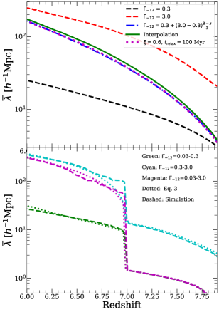
Figure 12: Tests of Eq. 3 using small-volume simulations with evolving $\Gamma_{\rm HI}$. Top: Test with $\Gamma_{\rm HI}(z)=0.3+(3.0-0.3)\frac{8-z}{3}$ (blue dot-dashed) alongside a direct interpolation between simulations with constant $\Gamma_{\rm HI}$ (green solid) and the result of evaluating Eq. 3 with $\xi=0.6$ and $t_{\rm relax}=100$ Myr (magenta dotted). The interpolation over-estimates $\overline{\lambda}$ by 10-15% while Eq. 3 produces agreement to within a few percent. Bottom: Tests in smaller ($0.256$ $h^{-1}$Mpc) volumes in which we impulsively increased $\Gamma_{\rm HI}$ by $1-2$ orders of magnitude at $z=7$. The dashed curves are the simulation results and the dotted curves are Eq. 3. The model agrees reasonably well even in these extreme cases, although the values of $\xi$ and $t_{\rm relax}$ vary between fits (and from our fiducial values).

Starting $\Gamma_{-12}$	Ending $\Gamma_{-12}$	${\bm{\xi}}$	${\bm{t}_{\rm relax}}$ [Myr]
0.03	0.3	0.8	700
0.3	3.0	0.33	100
0.03	3.0	0.67	300

Table 2: Best-fit parameters for our “impulsive-$\Gamma_{\rm HI}$” tests of Eq. 3, shown in Figure 12.

We also ran several tests (in smaller boxes) in which we increased $\Gamma_{\rm HI}$ impulsively by $1-2$ orders of magnitude midway through the simulation. These tests represent a “maximum stress test” of Eq. 3, since in reality $\Gamma_{\rm HI}$ will evolve more gradually. The bottom panel of Fig. 12 shows the result of three tests, with $\Gamma_{\rm HI}$ impulsively jumping between the values quoted in the legend at $z=7$. The dashed lines show the simulation results and the dotted lines the result of Eq. 3 (evaluated using a suite of similar simulations with constant $\Gamma_{-12}$). Though the values of $\xi$ and $t_{\rm relax}$ that gave these fits, given in Table 2, are somewhat different from each other (and our fiducial model), the goodness of the fits demonstrates the ability of Eq. 3 to capture $\overline{\lambda}$ in a variety of environments accurately. The variation may be due in part to the smaller box sizes of these tests and the fact that $\xi$ and $t_{\rm relax}$ are partially degenerate, but we also do expect that $\xi$ and $t_{\rm relax}$ should in general depend on $\Gamma_{\rm HI}$ (and, in principle, over-density and $z_{\rm reion}$). Future work will be required to address the environmental dependence of $\xi$ and $t_{\rm relax}$ in more detail.

References

- Abdurashidova et al. (2022a) Abdurashidova Z., et al., 2022a, ApJ, 924, 51
- Abdurashidova et al. (2022b) Abdurashidova Z., et al., 2022b, ApJ, 925, 221
- Abel & Wandelt (2002) Abel T., Wandelt B. D., 2002, MNRAS, 330, L53
- Ahn et al. (2015) Ahn K., Iliev I. T., Shapiro P. R., Srisawat C., 2015, MNRAS, 450, 1486
- Alvarez & Abel (2012) Alvarez M. A., Abel T., 2012, ApJ, 747, 126
- Barrow et al. (2020) Barrow K. S. S., Robertson B. E., Ellis R. S., Nakajima K., Saxena A., Stark D. P., Tang M., 2020, ApJ, 902, L39
- Becker & Bolton (2013) Becker G. D., Bolton J. S., 2013, MNRAS, 436, 1023
- Becker et al. (2015) Becker G. D., Bolton J. S., Madau P., Pettini M., Ryan-Weber E. V., Venemans B. P., 2015, MNRAS, 447, 3402
- Becker et al. (2018) Becker G. D., Davies F. B., Furlanetto S. R., Malkan M. A., Boera E., Douglass C., 2018, ApJ, 863, 92
- Becker et al. (2021) Becker G. D., D’Aloisio A., Christenson H. M., Zhu Y., Worseck G., Bolton J. S., 2021, MNRAS, 508, 1853
- Bianco et al. (2021) Bianco M., Iliev I. T., Ahn K., Giri S. K., Mao Y., Park H., Shapiro P. R., 2021, MNRAS, 504, 2443
- Bosman (2021) Bosman S. E. I., 2021, arXiv e-prints, p. arXiv:2108.12446
- Bosman et al. (2021) Bosman S. E. I., et al., 2021, arXiv e-prints, p. arXiv:2108.03699
- Bouwens et al. (2021) Bouwens R. J., et al., 2021, AJ, 162, 47
- Bullock et al. (2000) Bullock J. S., Kravtsov A. V., Weinberg D. H., 2000, ApJ, 539, 517
- Cain et al. (2021) Cain C., D’Aloisio A., Gangolli N., Becker G. D., 2021, ApJ, 917, L37
- Calverley et al. (2011) Calverley A. P., Becker G. D., Haehnelt M. G., Bolton J. S., 2011, Monthly Notices of the Royal Astronomical Society, 412, 2543
- Chen et al. (2022) Chen N., Trac H., Mukherjee S., Cen R., 2022, arXiv e-prints, p. arXiv:2203.04337
- Choudhury et al. (2021) Choudhury T. R., Paranjape A., Bosman S. E. I., 2021, MNRAS, 501, 5782
- Christenson et al. (2021) Christenson H. M., Becker G. D., Furlanetto S. R., Davies F. B., Malkan M. A., Zhu Y., Boera E., Trapp A., 2021, ApJ, 923, 87
- D’Aloisio et al. (2018) D’Aloisio A., McQuinn M., Davies F. B., Furlanetto S. R., 2018, MNRAS, 473, 560
- D’Aloisio et al. (2020) D’Aloisio A., McQuinn M., Trac H., Cain C., Mesinger A., 2020, The Astrophysical Journal, 898, 149
- Davies & Furlanetto (2016) Davies F. B., Furlanetto S. R., 2016, MNRAS, 460, 1328
- Davies & Furlanetto (2022) Davies F. B., Furlanetto S. R., 2022, MNRAS, 514, 1302
- Davies et al. (2018) Davies F. B., et al., 2018, The Astrophysical Journal, 864, 142
- Davies et al. (2021) Davies F. B., Bosman S. E. I., Furlanetto S. R., Becker G. D., D’Aloisio A., 2021, ApJ, 918, L35
- DeBoer et al. (2017) DeBoer D. R., et al., 2017, PASP, 129, 045001
- Doré et al. (2014) Doré O., et al., 2014, arXiv e-prints, p. arXiv:1412.4872
- Emami et al. (2019) Emami N., Siana B., Weisz D. R., Johnson B. D., Ma X., El-Badry K., 2019, ApJ, 881, 71
- Emberson et al. (2013) Emberson J. D., Thomas R. M., Alvarez M. A., 2013, The Astrophysical Journal, 763, 146
- Endsley et al. (2021) Endsley R., Stark D. P., Charlot S., Chevallard J., Robertson B., Bouwens R. J., Stefanon M., 2021, MNRAS, 502, 6044
- Fan et al. (2006) Fan X., et al., 2006, AJ, 132, 117
- Feng et al. (2018) Feng Y., Bird S., Anderson L., Font-Ribera A., Pedersen C., 2018, MP-Gadget/MP-Gadget: A tag for getting a DOI, doi:10.5281/zenodo.1451799, https://doi.org/10.5281/zenodo.1451799
- Finkelstein (2016) Finkelstein S. L., 2016, Publ. Astron. Soc. Australia, 33, e037
- Finkelstein et al. (2019) Finkelstein S. L., et al., 2019, ApJ, 879, 36
- Finlator et al. (2011) Finlator K., Davé R., Özel F., 2011, The Astrophysical Journal, 743, 169
- Furlanetto & Mirocha (2022) Furlanetto S. R., Mirocha J., 2022, MNRAS, 511, 3895
- Furlanetto & Oh (2005) Furlanetto S. R., Oh S. P., 2005, Monthly Notices of the Royal Astronomical Society, 363, 1031
- Garaldi et al. (2022) Garaldi E., Kannan R., Smith A., Springel V., Pakmor R., Vogelsberger M., Hernquist L., 2022, MNRAS,
- Gazagnes et al. (2021) Gazagnes S., Koopmans L. V. E., Wilkinson M. H. F., 2021, MNRAS, 502, 1816
- Giri et al. (2018) Giri S. K., Mellema G., Ghara R., 2018, MNRAS, 479, 5596
- Giri et al. (2019a) Giri S. K., Mellema G., Aldheimer T., Dixon K. L., Iliev I. T., 2019a, MNRAS, 489, 1590
- Giri et al. (2019b) Giri S. K., D’Aloisio A., Mellema G., Komatsu E., Ghara R., Majumdar S., 2019b, Journal of Cosmology and Astro-Particle Physics, 2019, 058
- Gnedin (2000) Gnedin N. Y., 2000, ApJ, 542, 535
- Gnedin (2014) Gnedin N. Y., 2014, ApJ, 793, 29
- Gnedin et al. (2011) Gnedin N. Y., Kravtsov A. V., Rudd D. H., 2011, ApJS, 194, 46
- Gorski et al. (1999) Gorski K. M., Wandelt B. D., Hansen F. K., Hivon E., Banday A. J., 1999, arXiv e-prints, pp astro–ph/9905275
- Greig et al. (2016) Greig B., Mesinger A., Haiman Z., Simcoe R. A., 2016, Monthly Notices of the Royal Astronomical Society, 466, 4239
- Greig et al. (2019) Greig B., Mesinger A., Bañados E., 2019, MNRAS, 484, 5094
- Greig et al. (2022) Greig B., Mesinger A., Davies F. B., Wang F., Yang J., Hennawi J. F., 2022, MNRAS, 512, 5390
- Hoeft et al. (2006) Hoeft M., Yepes G., Gottlöber S., Springel V., 2006, MNRAS, 371, 401
- Hu et al. (2019) Hu W., et al., 2019, ApJ, 886, 90
- Iliev et al. (2005a) Iliev I. T., Shapiro P. R., Raga A. C., 2005a, Monthly Notices of the Royal Astronomical Society, 361, 405
- Iliev et al. (2005b) Iliev I. T., Scannapieco E., Shapiro P. R., 2005b, ApJ, 624, 491
- Iliev et al. (2014) Iliev I. T., Mellema G., Ahn K., Shapiro P. R., Mao Y., Pen U.-L., 2014, MNRAS, 439, 725
- Ishimoto et al. (2022) Ishimoto R., et al., 2022, arXiv e-prints, p. arXiv:2207.05098
- Jung et al. (2020) Jung I., et al., 2020, ApJ, 904, 144
- Kannan et al. (2022) Kannan R., Garaldi E., Smith A., Pakmor R., Springel V., Vogelsberger M., Hernquist L., 2022, MNRAS, 511, 4005
- Kashikawa et al. (2006) Kashikawa N., et al., 2006, ApJ, 648, 7
- Kaur et al. (2020) Kaur H. D., Gillet N., Mesinger A., 2020, MNRAS, 495, 2354
- Keating et al. (2020a) Keating L. C., Weinberger L. H., Kulkarni G., Haehnelt M. G., Chardin J., Aubert D., 2020a, MNRAS, 491, 1736
- Keating et al. (2020b) Keating L. C., Kulkarni G., Haehnelt M. G., Chardin J., Aubert D., 2020b, MNRAS, 497, 906
- Koopmans et al. (2015) Koopmans L., et al., 2015, in Advancing Astrophysics with the Square Kilometre Array (AASKA14). p. 1 (arXiv:1505.07568), doi:10.22323/1.215.0001
- Kuhlen & Faucher-Giguère (2012) Kuhlen M., Faucher-Giguère C.-A., 2012, Monthly Notices of the Royal Astronomical Society, 423, 862
- Kulkarni et al. (2019) Kulkarni G., Keating L. C., Haehnelt M. G., Bosman S. E. I., Puchwein E., Chardin J., Aubert D., 2019, MNRAS, 485, L24
- Lewis et al. (2020) Lewis J. S. W., et al., 2020, MNRAS, 496, 4342
- Lewis et al. (2022) Lewis J. S. W., et al., 2022, arXiv e-prints, p. arXiv:2202.05869
- Maji et al. (2022) Maji M., et al., 2022, A&A, 663, A66
- Malloy & Lidz (2015) Malloy M., Lidz A., 2015, ApJ, 799, 179
- Mao et al. (2020) Mao Y., Koda J., Shapiro P. R., Iliev I. T., Mellema G., Park H., Ahn K., Bianco M., 2020, MNRAS, 491, 1600
- Marques-Chaves et al. (2022) Marques-Chaves R., et al., 2022, A&A, 663, L1
- Mason et al. (2018) Mason C. A., et al., 2018, ApJ, 857, L11
- Mason et al. (2019) Mason C. A., et al., 2019, Monthly Notices of the Royal Astronomical Society, 485, 3947
- Matthee et al. (2022) Matthee J., et al., 2022, MNRAS,
- McGreer et al. (2015) McGreer I. D., Mesinger A., D’Odorico V., 2015, MNRAS, 447, 499
- McQuinn & D’Aloisio (2018) McQuinn M., D’Aloisio A., 2018, JCAP, 2018, 016
- McQuinn et al. (2007) McQuinn M., Lidz A., Zahn O., Dutta S., Hernquist L., Zaldarriaga M., 2007, MNRAS, 377, 1043
- McQuinn et al. (2011) McQuinn M., Oh S. P., Faucher-Giguère C.-A., 2011, The Astrophysical Journal, 743, 82
- Mellema et al. (2013) Mellema G., et al., 2013, Experimental Astronomy, 36, 235
- Mesinger & Furlanetto (2007) Mesinger A., Furlanetto S., 2007, ApJ, 669, 663
- Mesinger et al. (2015) Mesinger A., Aykutalp A., Vanzella E., Pentericci L., Ferrara A., Dijkstra M., 2015, MNRAS, 446, 566
- Meyer et al. (2020) Meyer R. A., et al., 2020, MNRAS, 494, 1560
- Mirocha et al. (2021) Mirocha J., Plante P. L., Liu A., 2021, Monthly Notices of the Royal Astronomical Society, 507, 3872
- Mortlock et al. (2011) Mortlock D. J., et al., 2011, Nature, 474, 616
- Naidu et al. (2020) Naidu R. P., Tacchella S., Mason C. A., Bose S., Oesch P. A., Conroy C., 2020, ApJ, 892, 109
- Naidu et al. (2022) Naidu R. P., et al., 2022, MNRAS, 510, 4582
- Naoz & Barkana (2007) Naoz S., Barkana R., 2007, MNRAS, 377, 667
- Nasir & D’Aloisio (2020) Nasir F., D’Aloisio A., 2020, Monthly Notices of the Royal Astronomical Society, 494, 3080–3094
- Nasir et al. (2021) Nasir F., Cain C., D’Aloisio A., Gangolli N., McQuinn M., 2021, ApJ, 923, 161
- Ocvirk et al. (2016) Ocvirk P., et al., 2016, MNRAS, 463, 1462
- Ocvirk et al. (2021) Ocvirk P., Lewis J. S. W., Gillet N., Chardin J., Aubert D., Deparis N., Thélie É., 2021, MNRAS, 507, 6108
- Ono et al. (2011) Ono Y., et al., 2011, The Astrophysical Journal, 744, 83
- Ouchi et al. (2018) Ouchi M., et al., 2018, PASJ, 70, S13
- Park et al. (2016) Park H., Shapiro P. R., Choi J.-h., Yoshida N., Hirano S., Ahn K., 2016, ApJ, 831, 86
- Parsons et al. (2010) Parsons A. R., et al., 2010, AJ, 139, 1468
- Pentericci et al. (2014) Pentericci L., et al., 2014, The Astrophysical Journal, 793, 113
- Planck Collaboration et al. (2020) Planck Collaboration et al., 2020, A&A, 641, A6
- Qin et al. (2021) Qin Y., Mesinger A., Bosman S. E. I., Viel M., 2021, MNRAS, 506, 2390
- Robertson et al. (2015) Robertson B. E., Ellis R. S., Furlanetto S. R., Dunlop J. S., 2015, ApJ, 802, L19
- Ross et al. (2021) Ross H. E., Giri S. K., Mellema G., Dixon K. L., Ghara R., Iliev I. T., 2021, MNRAS, 506, 3717
- Schenker et al. (2012) Schenker M. A., Stark D. P., Ellis R. S., Robertson B. E., Dunlop J. S., McLure R. J., Kneib J.-P., Richard J., 2012, ApJ, 744, 179
- Shapiro et al. (1994) Shapiro P. R., Giroux M. L., Babul A., 1994, ApJ, 427, 25
- Shapiro et al. (2004) Shapiro P. R., Iliev I. T., Raga A. C., 2004, Monthly Notices of the Royal Astronomical Society, 348, 753
- Shukla et al. (2016) Shukla H., Mellema G., Iliev I. T., Shapiro P. R., 2016, MNRAS, 458, 135
- Sobacchi & Mesinger (2014) Sobacchi E., Mesinger A., 2014, MNRAS, 440, 1662
- Somerville & Davé (2015) Somerville R. S., Davé R., 2015, ARA&A, 53, 51
- Thoul & Weinberg (1996) Thoul A. A., Weinberg D. H., 1996, The Astrophysical Journal, 465, 608
- Tilvi et al. (2020) Tilvi V., et al., 2020, ApJ, 891, L10
- Tingay et al. (2013) Tingay S. J., et al., 2013, Publ. Astron. Soc. Australia, 30, e007
- Trac & Cen (2007) Trac H., Cen R., 2007, The Astrophysical Journal, 671, 1
- Trac & Pen (2004) Trac H., Pen U.-L., 2004, New Astron., 9, 443
- Trac et al. (2015) Trac H., Cen R., Mansfield P., 2015, ApJ, 813, 54
- Trac et al. (2022) Trac H., Chen N., Holst I., Alvarez M. A., Cen R., 2022, ApJ, 927, 186
- Vanzella et al. (2011) Vanzella E., et al., 2011, ApJ, 730, L35
- Wang et al. (2020) Wang F., et al., 2020, ApJ, 896, 23
- Watson et al. (2013) Watson W. A., Iliev I. T., D’Aloisio A., Knebe A., Shapiro P. R., Yepes G., 2013, MNRAS, 433, 1230
- Weisz et al. (2011) Weisz D. R., et al., 2011, The Astrophysical Journal, 744, 44
- Worseck et al. (2014) Worseck G., et al., 2014, MNRAS, 445, 1745
- Wu et al. (2019) Wu X., Kannan R., Marinacci F., Vogelsberger M., Hernquist L., 2019, MNRAS, 488, 419
- Wu et al. (2022) Wu P.-J., Xu Y., Zhang X., Chen X., 2022, ApJ, 927, 5
- Wyithe & Bolton (2011) Wyithe J. S. B., Bolton J. S., 2011, Monthly Notices of the Royal Astronomical Society, 412, 1926
- Xu et al. (2014) Xu Y., Yue B., Su M., Fan Z., Chen X., 2014, ApJ, 781, 97
- Xu et al. (2017) Xu Y., Yue B., Chen X., 2017, IAU Symp., 333, 64
- Yang et al. (2020) Yang J., et al., 2020, ApJ, 897, L14
- Yatawatta et al. (2013) Yatawatta S., et al., 2013, A&A, 550, A136
- Yeh et al. (2022) Yeh J. Y. C., et al., 2022, arXiv e-prints, p. arXiv:2205.02238
- Zhu et al. (2021) Zhu Y., et al., 2021, ApJ, 923, 223
- Zhu et al. (2022) Zhu Y., et al., 2022, ApJ, 932, 76