Weakly non-planar dimers

Abstract.

We study a model of fully-packed dimer configurations (or perfect matchings) on a bipartite periodic graph that is two-dimensional but not planar. The graph is obtained from $\mathbb{Z}^{2}$ via the addition of an extensive number of extra edges that break planarity (but not bipartiteness). We prove that, if the weight $\lambda$ of the non-planar edges is small enough, a suitably defined height function scales on large distances to the Gaussian Free Field with a $\lambda$-dependent amplitude, that coincides with the anomalous exponent of dimer-dimer correlations. Because of non-planarity, Kasteleyn’s theory does not apply: the model is not integrable. Rather, we map the model to a system of interacting lattice fermions in the Luttinger universality class, which we then analyze via fermionic Renormalization Group methods.

1. Introduction

The understanding of the rough phase of two-dimensional random interfaces is important in connection with the macroscopic fluctuation properties of equilibrium crystal shapes and of the separation surface between coexisting thermodynamic phases. A classical instance arises when studying the low temperature properties of the three-dimensional (3D) Ising model in the presence of Dobrushin Boundary Conditions (DBC). If DBC are fixed so to induce a horizontal interface between the $+$ and $-$ phases, it is well known [15] that at low enough temperatures the interface is rigid. It is conjectured that between the so-called roughening temperature and the Curie temperature, the interface displays fluctuations with unbounded variance (the variance diverges logarithmically with the system size), and the height profile supposedly has a massless Gaussian Free Field (GFF) behavior at large scales. This conjecture is completely open, in fact not even the existence of the roughening temperature has been proved. A connected result [20] is logarithmic divergence of fluctuations of the 2D SOS interface at large enough temperature; however, the result comes with no control of the scaling limit. If DBC are chosen so to induce a ‘tilted’ interface, say orthogonal to the $(1,1,1)$ direction, then things are different: fluctuations of the interface are logarithmic already at zero temperature; an exact mapping of the height profile and of its distribution into the dimer model on the hexagonal lattice, endowed with the uniform measure, allows one to get a full control on the large scale properties of the interface fluctuations, which are now proved to behave like a GFF (see [38] for the covariance structure, and [37], as well as [25, Section 3] for the full Gaussian limit). It is very likely that the GFF behavior survives the presence of a small but positive temperature; however, the techniques underlying the proof at zero temperature, based on the exact solvability of the planar dimer problem, break down. At positive temperatures, the very notion of height of the interface is not well defined, because of overhangs; these will have a low but non-zero density at low temperature. It is likely, though, that the height, even if not defined everywhere at a microscopic level, may be well-defined in a coarse grained sense; therefore, one can still ask about the large-scale behavior of its fluctuations. The coarse-grained height should admit an effective description in terms of a dimer model, whose distribution, however, is not expected to be uniform: temperature induces an effective ‘interaction’ among dimers.

In a previous series of works [25, 26, 27, 28], in collaboration with V. Mastropietro, we started developing methods for the treatment of non-solvable dimer models via constructive, fermionic, Renormalization Group (RG) techniques. We exhibited an explicit class of models, which include the 6-vertex model close to its free Fermi point as well as several non-integrable versions thereof, for which we proved scaling to the GFF, as well as the validity of a ‘Kadanoff’ or ‘Haldane’ scaling relation connecting the critical exponent of the so-called electric correlator with the one of the dimer-dimer correlation. Such a scaling relation is the counterpart, away from the free Fermi point, of the universality of the stiffness coefficient of the GFF first observed in [38], in connection with the fact that the spectral curve of a planar bipartite dimer model is a Harnack curve.

In this paper, motivated by our wish to understand the height fluctuations in situations where the height function is not locally well-defined at a microscopic level but only in a coarse-grained sense, as in the case of the 3D Ising interface discussed above, and in situations where the planarity assumption on the underlying graph fails to be satisfied, we generalize our analysis to a new setting, inspired by a problem proposed by S. Sheffield a few years ago. Namely, we study the large scale properties of a suitably defined height function, for a dimer model that is two-dimensional but non-planar. In short, we introduce a ‘weakly non-planar’ dimer model, by adding non-planar edges with small weights to a reference planar square lattice. We do so in a periodic fashion, and in such a way that non-planar edges are restricted to belong to cells, separated among each other by corridors of width one, which are crossed by none of the non-planar edges. The fact that non-planar edges avoid these corridors allows us to define a notion of height function on the faces belonging to the corridors themselves. We prove that this height function scales at large distances to a GFF with stiffness coefficient that is equal to the anomalous critical exponent of the two-point dimer-dimer correlation.

As in [25, 28], the proof is based on an exact representation of the dimer model as a system of interacting lattice fermions and in a rigorous multiscale analysis of the effective fermionic model, which has the structure of a lattice regularization of a Luttinger-type model. With respect to the previous works [25, 28], obtaining a fermionic representation turns out to be much less trivial, due to the loss of planarity. The infrared (i.e., large-scale) analysis of the lattice fermionic model is performed thanks to a comparison with a solvable reference continuum fermionic model, which has been studied and constructed in a series of works by G. Benfatto and V. Mastropietro [6, 7, 9, 10, 11, 12, 13], partly in collaboration also with P. Falco [6, 7, 8]. The GFF behavior and the Kadanoff-Haldane scaling relation of the dimer model follow from a careful comparison between the emergent chiral Ward Identities of the reference model with exact lattice Ward Identities of the dimer model.

The first novelty of the present work, as compared to [25, 26, 28], is related to the fermionic representation of the weakly non-planar model. The presence of non-planar edges requires a quite non-trivial adaptation of Kasteleyn’s theory, which is needed for the very formulation of the finite-volume model in terms of a non-Gaussian Grassmann integral. In fact, our non-planar model can in general be embedded on a surface of minimal genus $g\approx L^{2}$ (of the order of the number of non-planar edges) and Kasteleyn’s theory for the dimer model on general surfaces [21, 44] would express its partition function as the sum of $4^{g}$ determinants, i.e. of $4^{g}$ Gaussian Grassmann integrals, a rewriting that is not very useful for extracting thermodynamic properties. In this respect, the remarkable aspect of Proposition 1 below is that it expresses the partition function of just four Grassmann integrals, which are, however, non-Gaussian. The second novel ingredient of our construction is the identification (via the block-diagonalization procedure of Section 5.2) of massive modes associated with the Grassmann field which enters the fermionic representation of the model. The fact that the elementary cell of our model consists of $m^{2}$ sites, with $m$ an even integer larger or equal to $4$, implies that the basic Grassmann field of our effective model has a minimum of 16 components. It is well known [23, 45] that multi-component Luttinger models, such as the 1D Hubbard model [41], to cite the simplest possible example, do not necessarily display the same qualitative large distance features as the single-component one: new phenomena and quantum instabilities, such as spin-charge separation and metal-insulator transitions accompanied with the opening of a Mott gap may be present and may drastically change the resulting picture. Therefore, it is a priori unclear whether the height function of our model should still display a GFF behavior at large scales. Remarkably, however, the fact that the characteristic polynomial of the reference model has at most two simple zeros, as proven in [38], directly implies that all but two of the components of the effective Grassmann field are massive, and they can be preliminarily integrated out. This way, one can at last re-express the effective massless model in terms of just two massless fields (quasi-particle fields), in a way suitable for the application of the multi-scale analysis developed in [25, 28]. At this point, a large part of the multi-scale analysis is based on the tools developed in our previous works, which we will refer to for many technical aspects, without repeating the analysis in the present slightly different setting.

As a side remark, we emphasize that the massive modes would arise also in the “planar interacting dimer models” of [25, 28], if one worked on a graph whose fundamental cell contains $\ell\geq 2$ black/white vertices (an example is the square-octagon graph, see Fig. 5 in [38], where $\ell=4$). In contrast, one has $\ell=1$ in the context of [25, 28]. Our procedure consisting of (i) integrating out the massive degrees of freedom and (ii) reducing to an effective massless model, implies in particular that the results proved in [25, 28] for planar interacting dimer models on the square lattice extend to the case of general $\mathbb{Z}^{2}$-periodic two-dimensional bipartite lattices.

1.1. The broader context: height delocalization for discrete interface models

Recently, remarkable progress has been made on (logarithmic) delocalization of discrete, two-dimensional random interfaces. We start with the result which is maybe the closest in spirit to our work, that is [4, 5]. These works prove, by means of bosonic, constructive RG methods, that the height function of the discrete Gaussian interface model (that is the lattice GFF conditioned to be integer-valued) has, at sufficiently high temperature, the continuum GFF as scaling limit. In a way, this result is quite complementary to ours, since the model considered there is a perturbation of a free bosonic model (the lattice GFF), while in our case we perturb around a free fermionic one (the non-interacting dimer model). For closely related results on the 2D lattice Coulomb gas, see also [18, 19].

In a broader perspective, there has been a number of recent results (e.g. [1, 14, 40]) that prove delocalization of discrete, two-dimensional interface models at high temperature, even though they fall short of proving convergence to the GFF. Let us mention in particular the recent [40], which proves with a rather soft argument a (non-quantitative) delocalization statement for rather general height models, under the restriction, however, that the underlying graph has maximal degree three. For the particular case of the 6-vertex model, delocalization of the height function is known to hold in several regions of parameters [16, 17, 42, 46] but full scaling to the GFF has been proven only in a neighborhood of the free fermion point [28].

Organization of the article

The rest of the paper is organized as follows: in Section 2 we define the model and state our main results precisely. In Section 2 we review some useful aspects of Kasteleyn’s theory on toroidal graphs and derive the Grassmann representation of the weakly non-planar dimer model. In Section 4 we prove one of the main results of our work, concerning the logarithmic behavior of the height covariance at large distances and the Kadanoff-Haldane scaling relation, assuming temporarily a sharp asymptotic result on the correlation functions of the dimer model. The proof of the latter is based on a generalization of the analysis of [28], described in Section 5. As mentioned above, the novel aspect of this part consists in the identification and integration of the massive degrees of freedom (Sections 5.1-5.3), while the integration of the massless ones (Section 5.4) is completely analogous to the one described in [28]. Finally, in Section 6, we complete the proof of the convergence of the height function to the GFF.

2. Model and results

2.1. The “weakly non-planar” dimer model

To construct the graph $G_{L}$ on which our dimer model is defined, we let $L,m$ be two positive integers with $m\geq 4$ even, and we start with $G^{0}_{L}=(\mathbb{Z}/(Lm\,\mathbb{Z}))^{2}$, which is just the toroidal graph obtained by a periodization of $\mathbb{Z}^{2}$ with period $L\,m$ in both horizontal and vertical directions. We can partition $G^{0}_{L}$ into $L^{2}$ square cells $B_{x}$, $x=(x_{1},x_{2})\in\Lambda:=(-L/2,L/2]^{2}\cap\mathbb{Z}^{2}$, of sidelength $m$. The graph $G^{0}_{L}$ is plainly bipartite and we color vertices of the two sub-lattices black and white (each cell contains $m^{2}/2$ vertices of each color). Black (resp. white) vertices are denoted $b$ (resp. $w$). We let ${\bf e_{1}}$ (resp. ${\bf e_{2}}$) denote the horizontal (resp. vertical) vectors of length $m$ and we note that translation by ${\bf e_{1}}$ (resp. by ${\bf e_{2}}$) maps the cell $B_{x}$ into $B_{((x_{1}+1)\mod L,x_{2})}$ (resp. $B_{(x_{1},(x_{2}+1)\mod L)}$). A natural choice of coordinates for vertices is the following one: a vertex is identified by its color (black or white) and by a pair of coordinates $(x,\ell)$ where $x$ identifies the label of the cell the vertex belongs to, and the “type” $\ell\in\mathcal{I}:=\{1,\dots,m^{2}/2\}$ identifies the vertex within the cell. It does not matter how we label vertices within a cell, but we make the natural choice that if two vertices are related by a translation by a multiple of ${\bf e_{1},e_{2}}$, then they have the same type index $\ell$.

The graph $G_{L}$ is obtained from $G^{0}_{L}$ by adding in each cell $B_{x}$ a finite number of edges among vertices of opposite color (so that $G_{L}$ is still bipartite), with the constraint that $G_{L}$ is invariant under translations by multiples of ${\bf e_{1},e_{2}}$ (i.e., vertex $w$ of coordinates $(x,\ell)$ is joined to vertex $b$ of coordinates $(x,\ell^{\prime})$ if and only if the same holds for any other $x^{\prime}\in\Lambda$). See Fig. 1 for an example.

Remark 1.

It is easy to see that we need that $m\geq 4$ for this construction to work: if $m=2$, the two black edges in the cell are already connected to the two black vertices and there are no non-planar edges that can be added.

Note that $G_{L}$ is in general non-planar, even in the full-plane limit $L\to\infty$.

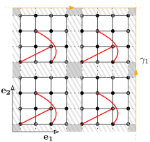
Figure 1. An example of graph $G_{L}$ with $L=2$, $m=4$ and two non-planar edges (in red) per cell. The height function is defined on the set $F$ of dashed faces outside of cells. Faces colored gray are those in $\bar{F}$ (they share a vertex with four different cells).

Let $E_{L}$ denote the set of edges of $G_{L}$: we write $E_{L}$ as the disjoint union $E_{L}=E^{0}_{L}\cup N_{L}$ where $E^{0}_{L}$ are the edges of $G^{0}_{L}$ (we call these “planar edges”) and $N_{L}$ (we call these “non-planar edges”) are the extra ones. Each edge $e\in E_{L}$ is assigned a positive weight: since we are interested in the situation where the weights of non-planar edges are small compared to those of planar edges, we first take a collection of weights $\{\tilde{t}_{e}\}_{e\in E_{L}},\tilde{t}_{e}>0$ that is invariant under translations by multiples of ${\bf e_{1},e_{2}}$, and then we establish that the weight of a planar edge $e$ is $t_{e}=\tilde{t}_{e}$ while that of a non-planar edge is $t_{e}=\lambda\tilde{t}_{e}$, where $\lambda$ is a real parameter, that will be taken small later.

To simplify expressions that follow, we will sometimes write ${\bf x}\in{\bf\Lambda}$ instead of $(x,\ell)\in\Lambda\times\mathcal{I}$ for the coordinate of a vertex of $G_{L}$. Also, we label the collection of edges in $E_{L}$ whose black vertex has type $\ell$ with a label $j\in\mathcal{J}_{\ell}=\{1,\dots,|\mathcal{J}_{\ell}|\}$. The labeling is done in such a way that two edges that are obtained one from the other via a translation by a multiple of ${\bf e_{1},e_{2}}$ have the same label. Note that $|\mathcal{J}_{\ell}|\geq 4$, and it is strictly larger than four if there are non-planar edges incident to the black vertex of type $\ell$. By convention, we label $j=1,\dots 4$ the four edges of $G^{0}_{L}$ belonging to $\mathcal{J}_{\ell}$, starting from the horizontal one whose left endpoint is black, and moving anti-clockwise.

The set of perfect matchings (or dimer configurations) of $G_{L}$ is denoted $\Omega_{L}$. Each $M\in\Omega_{L}$ is a subset of $E_{L}$ and the set of perfect matchings that contain only planar edges is denoted $\Omega^{0}_{L}$. Our main object of study is the probability measure on $\Omega_{L}$ given by

$$\mathbb{P}_{L,\lambda}(M)=\frac{w(M)}{Z_{L,{\bf\lambda}}}{\mathbbm{1}}_{M\in\Omega_{L}},\;w(M)=\prod_{e\in M}t_{e},\;Z_{L,\lambda}=\sum_{M\in\Omega_{L}}w(M).$$ (2.1)

We are interested in the limit where $L$ tends to infinity while $m$ (the cell size) is fixed. In this limit, the graph $G^{0}_{L}$ becomes the (planar) graph $G^{0}_{\infty}=\mathbb{Z}^{2}$ while $G_{L}$ becomes a periodic, bipartite but in general non-planar graph $G_{\infty}$. Cells $B_{x}$ of the infinite graphs are labelled by $x\in\mathbb{Z}^{2}$. We let $\Omega$ (resp. $\Omega^{0}$) denote the set of perfect matchings of $G_{\infty}$ (resp. of $\mathbb{Z}^{2}$).

In the case $\lambda=0$, the measure $\mathbb{P}_{L,0}$ is supported on $\Omega^{0}_{L}$: in fact, $\mathbb{P}_{L,0}$ is just the Boltzmann-Gibbs measure of the dimer model on the (periodized) square grid, with edge weights of periodicity $m$ (we will refer to this as the “non-interacting dimer model”). The non-interacting model is well understood via Kasteleyn’s [33, 34, 36] (and Temperley-Fisher’s [43]) theory, that allows to write its partition and correlation functions in determinantal form. According to the choice of the edge weights $\{t_{e}\}$, the non-interacting model can be either in a liquid (massless), gaseous (massive) or frozen phase, see [38]. In particular, in the liquid phase correlations decay like the squared inverse distance (see for instance (3.21)-(3.22) for a more precise statement). In this work, we assume that the edge weights are such that for $\lambda=0$, the model is in a massless phase.

The essential facts from Kasteleyn’s theory that are needed for the present work are recalled in Section 3.1. In particular, we emphasize that all the statistical properties of the non-interacting model are encoded in the so-called characteristic polynomial $\mu$ (see (3.9)), that is nothing else but the determinant of the Fourier transform of the so-called Kasteleyn matrix. Then, the assumption that the $\lambda=0$ model is in the massless phase, can be more precisely stated as follows:

Assumption 1.

The edge weights $\{t_{e}\}$ are such that the “characteristic polynomial” $\mu:[-\pi,\pi]^{2}\mapsto\mathbb{C}$ (see formula (3.9) below and the discussion following it) of the non-interacting dimer model has exactly two zeros $p^{+}_{0},p^{-}_{0}$ (distinct and simple).

We recall from [38] that this is a non-empty condition on the edge weights (in fact, this set of edge weights is a non-trivial open set). We also remark that if Assumption 1 is not satisfied, then we are in one of the following situations:

1. The edge weights are such that $\mu$ has no zeros on $[-\pi,\pi]^{2}$, corresponding to the frozen or to the gaseous phases of the non-interacting dimer model. In this case, the dimer model can be easily shown to be stable under the addition of dimer interaction such as those treated in [28] or of non-planar edges of small weight such as those treated in this paper. By ‘easily’, we mean ‘via a single-step fermionic cluster expansion’, which shows that the fluctuations of the perturbed model have the same qualitative behavior of the unperturbed ones. In this case, the height function displays no interesting behavior in the scaling limit.

2. The edge weights are such that $\mu$ has one double zero $p_{0}$ and: either the system is at the boundary separating the liquid from the gaseous or frozen phases (in which case $\nabla\mu(p_{0})\neq 0$), or it is at a degenerate point within the liquid phase (in which case, called ‘real node’ in [38], $\nabla\mu(p_{0})=0$). These cases display rich and interesting behaviors: e.g., the fluctuations of the height level lines of the integrable dimer model, close to the liquid/frozen and liquid/gaseous boundaries converge to the so-called Airy process [3, 32]. We postpone the analysis of non-integrable dimer models in such critical cases to future work.

2.2. Results

Our main goal is to understand the large-scale properties of the height function under the limit measure $\mathbb{P}_{\lambda}$, which is the weak limit as $L\to\infty$ of $\mathbb{P}_{L,\lambda}$. The fact that this limit exists, provided that $|\lambda|\leq\lambda_{0}$ for a sufficiently small $\lambda_{0}$, is a byproduct of the proof.

Our first main result concerns the large distance asymptotics of the truncated dimer-dimer correlations. We use the notation $\mathds{1}_{e}$ for the indicator function that the edge $e$ is occupied by a dimer, and $\mathbb{E}_{\lambda}(f;g)$ for $\mathbb{E}_{\lambda}(fg)-\mathbb{E}_{\lambda}(f)\mathbb{E}_{\lambda}(g)$.

Theorem 1.

Choose the dimer weights on the planar edges as in Assumption 1. There exists $\lambda_{0}>0$ and analytic functions $\nu:[-\lambda_{0},\lambda_{0}]\mapsto\mathbb{R}^{+}$, $\alpha_{\omega},\beta_{\omega}:[-\lambda_{0},\lambda_{0}]\mapsto\mathbb{C}\setminus\{0\}$ (labelled by $\omega\in\{+,-\}$ and satisfying $\overline{\alpha_{+}}=-\alpha_{-},\overline{\beta_{+}}=-\beta_{-}$ and $\alpha_{\omega}(\lambda)/\beta_{\omega}(\lambda)\not\in\mathbb{R}$), $K_{\omega,j,\ell},H_{\omega,j,\ell}:[-\lambda_{0},\lambda_{0}]\mapsto\mathbb{C}$ (labelled by $\omega\in\{+,-\}$, $\ell\in\mathcal{I}$, $j\in\mathcal{J}_{\ell}$ and satisfying $K_{\omega,j,\ell}=\overline{K_{-\omega,j,\ell}}$, $H_{\omega,j,\ell}=\overline{H_{-\omega,j,\ell}}$) and $p^{\omega}:[-\lambda_{0},\lambda_{0}]\mapsto[-\pi,\pi]^{2}$ (labelled by $\omega\in\{-1,+1\}$ and satisfying $p^{+}=-p^{-}$) such that, for any two edges $e,e^{\prime}$ with black vertices $(x,\ell),(x^{\prime},\ell^{\prime})\in\mathbb{Z}^{2}\times\mathcal{I}$ such that $x\neq x^{\prime}$ and labels $j\in\mathcal{J}_{\ell}$, $j^{\prime}\in\mathcal{J}_{\ell^{\prime}}$,

$$\mathbb{E}_{\lambda}(\mathds{1}_{e};\mathds{1}_{e^{\prime}})=\sum_{\omega}\Biggl{[}\frac{K_{\omega,j,\ell}K_{\omega,j^{\prime},\ell^{\prime}}}{(\phi_{\omega}(x-x^{\prime}))^{2}}+\frac{H_{\omega,j,\ell}H_{-\omega,j^{\prime},\ell^{\prime}}}{|\phi_{\omega}(x-x^{\prime})|^{2\nu}}e^{2ip^{\omega}\cdot(x-x^{\prime})}\Biggr{]}+\text{Err}(e,e^{\prime}),$$ (2.2)

where, letting $x=(x_{1},x_{2})$,

$$\phi_{\omega}(x):=\omega(\beta_{\omega}(\lambda)x_{1}-\alpha_{\omega}(\lambda)x_{2})$$ (2.3)

and $|\text{Err}(e,e^{\prime})|\leq C|x-x^{\prime}|^{-3+O(\lambda)}$ for some $C>0$ and $O(\lambda)$ independent of $x,x^{\prime}$. Moreover, $\nu(\lambda)=1+O(\lambda)$.

Even if not indicated explicitly, the functions $\nu,\alpha_{\omega},\beta_{\omega},K_{\omega,j,\ell},H_{\omega,j,\ell},p^{\omega}$ all depend non-trivially on the edge weights $\{t_{e}\}$. In particular, generically, $\nu=1+c_{1}\lambda+O(\lambda^{2})$, with $c_{1}$ a non zero coefficient, which depends upon the edge weights (this was already observed in [27] for interacting dimers on planar graphs); therefore, generically, $\nu$ is larger or smaller than $1$, depending on the sign of $\lambda$.

At $\lambda=0$, (2.2) reduces to the known asymptotic formula for the truncated dimer-dimer correlation of the standard planar dimer model, which is reviewed in the next section. The most striking difference between the case $\lambda\neq 0$ and $\lambda=0$ is the presence of the critical exponent $\nu$ in the second term in square brackets in the right hand side of (2.2). It shows that the presence of non-planar edges in the model qualitatively changes the large distance decay properties of the dimer-dimer correlations. Therefore, naive universality, in the strong sense that all critical exponents of the perturbed model are the same as those of the reference unperturbed one, fails. In the present context the correct notion to be used is that of ‘weak universality’, due to Kadanoff, on the basis of which we expect that the perturbed model is characterized by a number of exact scaling relations; these should allow us to reduce all the non-trivial critical exponents of the model (i.e., those depending continuously on the strength of the perturbation) to just one of them, for instance $\nu$ itself. A rigorous instance of such a scaling is discussed in Remark 2 below.

The weak universality picture is formally predicted by bosonization methods (see the introduction of [26] for a brief overview), which allow one to express the large distance asymptotics of all correlation functions in terms of a single, underlying, massless GFF. Such a GFF is nothing but the scaling limit of the height function of the model, as discussed in the following. Given a perfect matching $M\in\Omega^{0}$ of the infinite graph $G^{0}_{\infty}=\mathbb{Z}^{2}$, there is a standard definition of height function on the dual graph: given two faces $\xi,\eta$ of $\mathbb{Z}^{2}$, one defines

$$h(\eta)-h(\xi)=\sum_{e\in C_{\xi\to\eta}}\sigma_{e}\Big{(}\mathbbm{1}_{e\in M}-\frac{1}{4}\Big{)}$$ (2.4)

together with $h(\xi_{0})=0$ at some reference face $\xi_{0}$. Here, $C_{\xi\to\eta}$ is a nearest-neighbor path from $\xi$ to $\eta$ and $\sigma_{e}$ is a sign which equals $+1$ if the edge $e$ is crossed with the white vertex on right and $-1$ otherwise). The definition is well-posed since it is independent of the choice of the path. We recall that under $\mathbb{P}_{0}$, the height function is known to admit a GFF scaling limit [37, 25].

A priori, on a non-planar graph such as $G$, there is no canonical bijection between perfect matchings and height functions. However, since the non-planarity is “local” (non-planar edges do not connect different cells), there is an easy way out. Namely, let $F$ denote the set of faces of $\mathbb{Z}^{2}$ that do not belong to any of the cells $B_{x}$ (see Figure 1). Given a perfect matching $M\in\Omega$, define an integer-valued height function $h$ on faces $\xi\in F$ by setting it to zero at some reference face $\xi_{0}\in F$ and by imposing (2.4) for any path $C_{\xi\to\eta}$ that uses only faces in $F$. It is easy to check that $h$ is then independent of the choice of path.

Our second main result implies in particular that the variance of the height difference between faraway faces in $F$ grows logarithmically with the distance. For simplicity, let us restrict our attention to the subset $\bar{F}\subset F$ of faces that share a vertex with four cells (see Fig. 1): if a face in $\bar{F}$ shares a vertex with $B_{x},B_{x-(0,1)},B_{x-(1,0)},B_{x-(1,1)}$, then we denote it by $\eta_{x}$.

Theorem 2.

Under the same assumptions as Theorem 1, for $x^{(1)},\dots,x^{(4)}\in\mathbb{Z}^{2}$,

$$\mathbb{E}_{\lambda}\left[(h(\eta_{x^{(1)}})-h(\eta_{x^{(2)}}));(h(\eta_{x^{(3)}})-h(\eta_{x^{(4)}}))\right]\\ =\frac{\nu(\lambda)}{2\pi^{2}}\Re\left[\log\frac{(\phi_{+}({x^{(4)}})-\phi_{+}({x^{(1)}}))(\phi_{+}({x^{(3)}})-\phi_{+}({x^{(2)}}))}{(\phi_{+}({x^{(4)}})-\phi_{+}({x^{(2)}}))(\phi_{+}({x^{(3)}})-\phi_{+}({x^{(1)}}))}\right]\\ +O\left(\frac{1}{\min_{i\neq j\leq 4}|x^{(i)}-x^{(j)}|^{1/2}+1}\right)$$ (2.5)

where $\nu$ and $\phi_{+}$ are the same as in Theorem 1

Note that in particular, taking $x^{(1)}=x^{(3)}=x,x^{(2)}=x^{(4)}=y$ we have

$${\rm Var}_{\mathbb{P}_{\lambda}}(h(\eta_{x})-h(\eta_{y}))=\frac{\nu(\lambda)}{\pi^{2}}\Re\log(\phi_{+}(x)-\phi_{x}(y))+O(1)=\frac{\nu(\lambda)}{\pi^{2}}\log|x-y|+O(1)$$ (2.6)

as $|x-y|\to\infty$.

Remark 2.

The remarkable fact of this result is that the ‘stiffness’ coefficient $\nu(\lambda)/\pi^{2}$ of the GFF is the same, up to the $1/\pi^{2}$ factor, as the critical exponent of the oscillating part of the dimer-dimer correlation. There is no a priori reason that the two coefficients should be the same, and it is actually a deep implication of our proof that this is the case. Such an identity is precisely one of the scaling relations predicted by Kadanoff and Haldane in the context of the 8-vertex, Ashkin-Teller, XXZ, and Luttinger liquid models, which are different models in the same universality class as our non-planar dimers (see [26] for additional discussion and references).

Building upon the proof of Theorem 2, we also obtain bounds on the higher point cumulants of the height; these, in turn, imply convergence of the height profile to a massless GFF:

Theorem 3.

Assume that $|\lambda|\leq\lambda_{0}$, with $\lambda_{0}>0$ as in Theorem 2. For every $C^{\infty}$, compactly supported test function $f:\mathbb{R}^{2}\mapsto\mathbb{R}$ of zero average and $\epsilon>0$, define

$$h^{\epsilon}(f):=\epsilon^{2}\sum_{x\in\mathbb{Z}^{2}}\big{(}h(\eta_{x})-\mathbb{E}_{\lambda}(h(\eta_{x}))\big{)}f(\epsilon x).$$ (2.7)

Then, one has the convergence in distribution

$$h^{\epsilon}(f)\stackrel{{\scriptstyle\epsilon\to 0}}{{\Longrightarrow}}\mathcal{N}(0,\sigma^{2}(f))$$ (2.8)

where $\mathcal{N}(0,\sigma^{2}(f))$ denotes a centered Gaussian distribution of variance

$$\sigma^{2}(f):=\frac{\nu(\lambda)}{2\pi^{2}}\int_{\mathbb{R}^{2}}dx\int_{\mathbb{R}^{2}}dyf(x)\Re[\log\phi_{+}(x-y)]f(y).$$

3. Grassmann representation of the generating function

In this section we rewrite the partition function $Z_{L,\lambda}$ of (2.1) in terms of Grassmann integrals (see Sect.3.3). As a byproduct of our construction, we obtain a similar Grassmann representation for the generating function of correlations of the dimer model. We also observe that the Grassmann integral for the generating function is invariant under a lattice gauge symmetry, whose origin has to be traced back to the local conservation of the number of incident dimers at lattice sites, and which implies exact lattice Ward Identities for the dimer correlations (see Sect.3.4).

Before diving into the proof of the Grassmann representation, it is convenient to recall some preliminaries about the planar dimer model, its Gaussian Grassmann representation and the structure of its correlation functions in the thermodynamic limit. This will be done in the next two subsection, Sect.3.1, 3.2

3.1. A brief reminder of Kasteleyn theory

Here we recall a few basic facts of Kasteleyn theory for the dimer model on a bipartite graph $G=(V,E)$ embedded on the torus, with edge weights $\{t_{e}>0\}_{e\in E}$. For later purposes, we need this for more general such graphs than just $G^{0}_{L}$. For details we refer to [21], which considers the more general case where the graph is not bipartite and it is embedded on an orientable surface of genus $g\geq 1$. For the considerations of this section, we do not need the edge weights to display any periodicity, so here we will work with generic, not necessarily periodic, edge weights.

As in [21], we assume that $G$ can be represented as a planar connected graph $G_{0}=(V,E_{0})$ (we call this the “basis graph of $G$”), embedded on a square, with additional edges that connect the two vertical sides of the square (edges $E_{1}$) or the two horizontal sides (edges $E_{2}$). Note that $E=E_{0}\cup E_{1}\cup E_{2}$. See Figure 2. We always assume that the basis graph $G_{0}$ is connected and actually that it is $2-$connected (i.e. removal of any single vertex together with the edges attached to it does not make $G_{0}$ disconnected). We also assume that $G_{0}$ admits at least one perfect matching and we fix a reference one, which we call $M_{0}$.

Following the terminology of [21], we introduce the following definition.

Definition 1 (Basic orientation).

We call an orientation $D_{0}$ of the edges $E_{0}$ a “basic orientation of $G_{0}$” if all the internal faces of the basis graph $G_{0}$ are clock-wise odd, i.e. if running clockwise along the boundary of the face, the number of co-oriented edges is odd (since $G_{0}$ is 2-connected, the boundary of each face is a cycle).

A basic orientation always exists [21], but in general it is not unique. Next, one defines $4$ orientations of the full graph $G$ as follows (these are called “relevant orientations” in [21]). First, one draws the planar graphs $G_{j},j=1,2$ whose edge sets are $E_{0}\cup E_{j}$, as in Fig. 2.

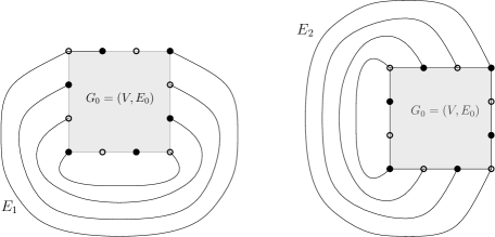
Figure 2. The basis graph $G_{0}$ is schematically represented by the gray square (the vertices and edges inside the square are not shown). In the left (resp. right) drawing is pictured the planar graph $G_{1}$ (resp. $G_{2}$)

Note that there is a unique orientation $D_{j}$ of the edges in $E_{0}\cup E_{j}$ that coincides with $D_{0}$ on $E_{0}$ and such that all the internal faces of $G_{j}$ are clockwise odd. Then, we define the relevant orientation $D_{\theta}$ of type $\theta=(\theta_{1},\theta_{2})\in\{-1,+1\}^{2}$ of $G$ as the unique orientation of the edges $E$ that coincides with $D_{0}$ on $G_{0}$ and with $\theta_{1}D_{j}$ on the edges in $E_{j},j=1,2$. Given one of the four relevant orientations $D_{\theta}$ of $G$, we define a $|V|\times|V|$ antisymmetric matrix $A_{D_{\theta}}$ by establishing that for $v,v^{\prime}\in V$, $A_{D_{\theta}}(v,v^{\prime})=0$ if $(v,v^{\prime})\not\in E$, while $A_{D_{\theta}}(v,v^{\prime})=t_{e}$ if $v,v^{\prime}$ are the endpoint of the edge $e$ oriented from $v$ to $v^{\prime}$, and $A_{D_{\theta}}(v,v^{\prime})=-t_{e}$ if $e$ is oriented from $v^{\prime}$ to $v$. Then, [21, Corollary 3.5] says that

$$Z_{G}=\sum_{M\in\Omega_{G}}w(M)=\sum_{\theta\in\{-1,+1\}^{2}}\frac{c_{\theta}}{2}\frac{{\rm Pf}(A_{D_{\theta}})}{s(M_{0})}$$ (3.1)

where $\Omega_{G}$ is the set of the perfect matchings of $G$, $w(M)=\prod_{e\in M}t_{e}$, and

$$c_{(-1,-1)}=-1\text{ and }c_{\theta}=1\text{ otherwise.}$$ (3.2)

In (3.1), ${\rm Pf}(A)$ denotes the Pfaffian of an anti-symmetric matrix $A$ and $s(M_{0})$ denotes the sign of the term corresponding to the reference matching $M_{0}$ in the expansion of the Pfaffian ${\rm Pf}(A_{D_{\theta}})$. Since by assumption $M_{0}$ contains only edges from $E_{0}$ whose orientation does not depend on $\theta$, $s(M_{0})$ is indeed independent of $\theta$.

In our case, in contrast with the general case considered in [21], the graph $G$ is bipartite. By labeling the vertices so that the first $|V|/2$ are black and the last $|V|/2$ are white, the matrices $A_{D_{\theta}}(v,v^{\prime})$ have then a block structure of the type

$$A_{D_{\theta}}=\begin{pmatrix}0&\vline&+K_{\theta}\\ \hline\cr-K_{\theta}&\vline&0\end{pmatrix}$$ (3.3)

We view the $|V|/2\times|V|/2$ “Kasteleyn matrices” $K_{\theta}$ as having rows indexed by black vertices and columns by white vertices.

By using the relation [30, Eq. (16)] between Pfaffians and determinants, one can then rewrite the above formula as

$$Z_{G}=\sum_{\theta\in\{-1,+1\}^{2}}\frac{\tilde{c}_{\theta}}{2}\det(K_{\theta}),\quad\tilde{c}_{\theta}=c_{\theta}\frac{(-1)^{(|V|/2-1)|V|/4}}{s(M_{0})}.$$ (3.4)

Remark 3.

Note that changing the order in the labeling of the vertices changes the sign $s(M_{0})$. We suppose henceforth that the choice is done so that the ratio in the definition of $\tilde{c}_{\theta}$ equals $1$, so that $\tilde{c}_{\theta}=c_{\theta}$.

3.2. Thermodynamic limit of the planar dimer model

In the previous section, Kasteleyn’s theory for rather general toroidal bipartite graphs was recalled, without assuming any type of translation invariance. In this subsection, instead, we specialize to $G=G^{0}_{L}$ (the periodized version of $\mathbb{Z}^{2}$ introduced in Section 2.1) and, as was the case there, we assume that the edge weights are invariant under translations by multiples of ${\bf e_{1},\bf e_{2}}$.

With Kasteleyn’s theory at hand, one can compute the thermodynamic and large-scale properties of the dimer model on $G^{0}_{L}$ as $L\to\infty$. We refer to [38, 37, 29] for details. In the case where $G=G^{0}_{L}$, the basis graph $G_{0}$ is a square grid with $Lm$ vertices per side and we choose its basic orientation $D_{0}$ so that horizontal edges are oriented from left to right, while vertical edges are oriented from bottom to top on every second column and from top to bottom on the remaining columns. With this choice, the orientations $D_{1},D_{2}$ of $G_{1},G_{2}$ are like in Fig. 3. Note that, if $e=(b,w)\in E_{L}^{0}$ is an edge of $G_{L}^{0}$, then for $\theta=(\theta_{1},\theta_{2})\in\{-1,+1\}^{2}$, $K_{\theta}(b,w)$ equals $K_{(+1,+1)}(b,w)$ multiplied by $(-1)^{(\theta_{1}-1)/2}$ if $e$ belongs to $E_{1}$ (see Fig. 2) and by $(-1)^{(\theta_{2}-1)/2}$ if $e$ belongs to $E_{2}$.

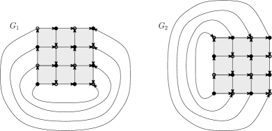
Figure 3. The graphs $G_{1},G_{2}$ corresponding to the basis graph of $G_{L}^{0}$ (for $L\,m=4$), together with their orientations $D_{1},D_{2}$.

Observe also that the matrix $K_{(-1,-1)}$ is invariant under translations by multiples of ${\bf e_{1},e_{2}}$. Define

$$\mathcal{P}(\theta):=\left\{k=(k_{1},k_{2}):k_{j}=\frac{2\pi}{L}\left(n_{j}+\frac{\theta_{j}+1}{4}\right),-L/2<n_{j}\leq L/2\right\}.$$ (3.5)

Let $P_{\theta}$ be the orthogonal $(Lm)^{2}/2\times(Lm)^{2}/2$ matrix whose columns are indexed by $(k,\ell),k\in\mathcal{P}(\theta),\ell\in\mathcal{I}=\{1,\dots,m^{2}/2\}$, whose rows are indexed by $(x,\ell),x\in\Lambda,\ell\in\mathcal{I}$, and such that the column indexed $(k,\ell)$ is the vector

$$f_{\ell,k}:((x,\ell^{\prime})\in\Lambda\times\mathcal{I})\mapsto f_{\ell,k}(x,\ell^{\prime})=\frac{1}{L}e^{-ikx}{\bf 1}_{\ell^{\prime}=\ell}.$$ (3.6)

Then, $P_{\theta}^{-1}K_{\theta}P_{\theta}$ is block-diagonal with blocks of size $|\mathcal{I}|$ labelled by $k\in\mathcal{P}(\theta)$. The block corresponding to the value $k$ is a $|\mathcal{I}|\times|\mathcal{I}|$ matrix $M(k)$ of elements $[M(k)]_{\ell,\ell^{\prime}}$ with $\ell,\ell^{\prime}\in\mathcal{I}$ and

$$[M(k)]_{\ell,\ell^{\prime}}=\sum_{e:\ell\stackrel{{\scriptstyle e}}{{\sim}}\ell^{\prime}}K_{(-1,-1)}(b,w)e^{-ikx_{e}}.$$ (3.7)

In this formula, the sum runs over all edges $e$ joining the black vertex $b$ of type $\ell$ in the cell of coordinates $x=(0,0)$ to some white vertex $w$ of type $\ell^{\prime}$ ($w$ can be either in the same fundamental cell or in another one); $x_{e}\in\mathbb{Z}^{2}$ is the coordinate of the cell to which $w$ belongs.

The thermodynamic and large-scale properties of the measure $\mathbb{P}_{L,0}$ are encoded in the matrix $M$: for instance the infinite volume free energy exists and it is given by [38]

$$F=:\lim_{L\to\infty}\frac{1}{L^{2}}\log Z_{L,0}=\frac{1}{(2\pi)^{2}}\int_{[-\pi,\pi]^{2}}\log|\mu(k)|dk$$ (3.8)

where $\mu$ (the “characteristic polynomial”) is

$$\mu(k):=\det M(k),$$ (3.9)

which is a polynomial in $e^{ik_{1}},e^{ik_{2}}$. Kasteleyn’s theory allows one to write multi-point dimer correlations (in the $L\to\infty$ limit) in terms of the so-called “infinite-volume inverse Kasteleyn matrix” $K^{-1}$: if $w$ (resp. $b$) is a white (resp. black) vertex of type $\ell$ in cell $x=(x_{1},x_{2})\in\mathbb{Z}^{2}$ (resp. of type $\ell^{\prime}$ and in cell $0$), then one has

$$K^{-1}(w,b):=\frac{1}{(2\pi)^{2}}\int_{[-\pi,\pi]^{2}}[(M(k))^{-1}]_{\ell,\ell^{\prime}}e^{-ikx}dk.$$ (3.10)

As can be guessed from (3.10), the long-distance behavior of $K^{-1}$ is related to the zeros of the determinant of $M(k)$, that is, to the zeros of $\mu$ on $[-\pi,\pi]^{2}$. It is a well known fact [38] that, for any choice of the edge weights, $\mu$ can have at most two zeros. Our Assumption 1 means that we restrict to a choice of edge weights such that $\mu$ has exactly two zeros, named $p_{0}^{+},p_{0}^{-}$, with $p_{0}^{+}\neq p^{-}_{0}\mod(2\pi,2\pi)$. We also define the complex numbers

$$\alpha^{0}_{\omega}:=\partial_{k_{1}}\mu(p_{0}^{\omega}),\quad\beta^{0}_{\omega}:=\partial_{k_{2}}\mu(p_{0}^{\omega}),\quad\omega=\pm.$$ (3.11)

Note that, since the Kasteleyn matrix elements $K_{\theta}(b,w)$ are real, from (3.7) we have the symmetry

$$[M(-k)]_{\ell,\ell^{\prime}}=\overline{[M(k)]_{\ell\ell^{\prime}}}$$ (3.12)

and in particular

$$p_{0}^{+}+p_{0}^{-}=0$$ (3.13)

$$\alpha^{0}_{-}=-\overline{\alpha^{0}_{+}},\quad\beta^{0}_{-}=-\overline{\beta^{0}_{+}}.$$ (3.14)

It is also known [38] that $\alpha^{0}_{\omega},\beta^{0}_{\omega}$ are not collinear as elements of the complex plane:

$$\alpha^{0}_{\omega}/\beta^{0}_{\omega}\not\in\mathbb{R}.$$ (3.15)

Note that from (3.14) it follows that $\text{Im}(\beta_{+}^{0}/\alpha_{+}^{0})=-\text{Im}(\beta_{-}^{0}/\alpha_{-}^{0})$. From now on, with no loss of generality, we assume that

$$\text{Im}(\beta_{+}^{0}/\alpha_{+}^{0})>0,$$ (3.16)

which amounts to choosing appropriately the labels $+,-$ associated with the two zeros of $\mu(k)$.

If we denote by $\operatorname{adj}(A)$ the adjugate of the matrix $A$, so that $A^{-1}=\operatorname{adj}(A)/\det A$, the long-distance behavior of the inverse Kasteleyn matrix is given [38] as

$$K^{-1}(w,b)\stackrel{{\scriptstyle|x|\to\infty}}{{=}}\frac{1}{2\pi}\sum_{\omega=\pm}[\operatorname{adj}(M(p^{\omega}))]_{\ell,\ell^{\prime}}\frac{e^{-ip_{0}^{\omega}x}}{\phi^{0}_{\omega}(x)}+O(|x|^{-2})$$ (3.17)

where

$$\phi^{0}_{\omega}(x)=\omega(\beta^{0}_{\omega}x_{1}-\alpha^{0}_{\omega}x_{2}).$$ (3.18)

Note that since the zeros $p_{0}^{\omega}$ of $\mu(k)$ are simple, the matrix $\operatorname{adj}M(p_{0}^{\omega})$ has rank $1$. This means that we can write

$$\operatorname{adj}M(p_{0}^{\omega})=U^{\omega}\otimes V^{\omega}$$ (3.19)

for vectors $U^{\omega},V^{\omega}\in\mathbb{C}^{|\mathcal{I}|}$, where $\otimes$ is the Kronecker product. Let $e=(b,w),e^{\prime}=(b^{\prime},w^{\prime})$ be two fixed edges of $G^{0}_{L}$: we assume that the black endpoint of $e$ (resp. of $e^{\prime}$) has coordinates ${\bf x}=(x,\ell)$ (resp. ${\bf x^{\prime}}=(x^{\prime},\ell^{\prime})$) and that the white endpoint of $e$ (resp. $e^{\prime}$) has coordinates $(x+v(e),m)$ with $m\in\mathcal{I}$ (resp. coordinates $(x^{\prime}+v(e^{\prime}),m^{\prime})$). Of course, $v(e)$ is either $(0,0)$ or $(0,\pm 1)$ or $(\pm 1,0)$, and similarly for $v(e^{\prime})$. Note that the coordinates of the white endpoint of $e$ are uniquely determined by the coordinates of the black endpoint and the orientation label $j\in\{1,\dots,4\}$ of $e$: in this case we will write $v(e)=:v_{j,\ell}$, $K(b,w)=:K_{j,\ell}$ and in (3.19), $U_{m}=:U_{j,\ell}$. The (infinite-volume) truncated dimer-dimer correlation under the measure $\mathbb{P}_{L,0}$ is given as

$$\mathbb{E}_{0}({\mathbbm{1}}_{e};{\mathbbm{1}}_{e^{\prime}})=\lim_{L\to\infty}\mathbb{E}_{L,0}({\mathbbm{1}}_{e};{\mathbbm{1}}_{e^{\prime}})=-K(b,w)K(b^{\prime},w^{\prime})K^{-1}(w^{\prime},b)K^{-1}(w,b^{\prime}).$$ (3.20)

As a consequence of the asymptotic expression (3.17), we have that as $|x^{\prime}-x|\to\infty$,

$$\mathbb{E}_{0}[{\mathbbm{1}}_{e};{\mathbbm{1}}_{e^{\prime}}]=A_{j,\ell,j^{\prime},\ell^{\prime}}(x,x^{\prime})+B_{j,\ell,j^{\prime},\ell^{\prime}}(x,x^{\prime})+R^{0}_{j,\ell,j^{\prime},\ell^{\prime}}(x,x^{\prime})$$ (3.21)

with

$$\begin{split}A_{j,\ell,j^{\prime},\ell^{\prime}}(x,x^{\prime})&=\sum_{\omega=\pm}\frac{K^{0}_{\omega,j,\ell}K^{0}_{\omega,j^{\prime},\ell^{\prime}}}{(\phi^{0}_{\omega}(x-x^{\prime}))^{2}}\\ B_{j,\ell,j^{\prime},\ell^{\prime}}(x,x^{\prime})&=\sum_{\omega=\pm}\frac{H^{0}_{\omega,j,\ell}H^{0}_{-\omega,j^{\prime},\ell^{\prime}}}{|\phi^{0}_{\omega}(x-x^{\prime})|^{2}}e^{2ip_{0}^{\omega}(x-x^{\prime})}\\ |R^{0}_{j,\ell,j^{\prime}\ell^{\prime}}(x,x^{\prime})|&\leq C|x-x^{\prime}|^{-3}.\end{split}$$ (3.22)

where

$$\begin{split}&K^{0}_{\omega,j,\ell}:=\frac{1}{2\pi}K_{j,\ell}e^{-ip_{0}^{\omega}v_{j,\ell}}U^{\omega}_{j,\ell}V^{\omega}_{\ell}\\ &H^{0}_{\omega,j,\ell}:=\frac{1}{2\pi}K_{j,\ell}e^{ip_{0}^{\omega}v_{j,\ell}}U^{-\omega}_{j,\ell}V^{\omega}_{\ell}.\end{split}$$ (3.23)

3.3. A fermionic representation for $Z_{L,\lambda}$

In this subsection, we work again with generic edge weights, i.e., we do not assume that they have any spatial periodicity.

3.3.1. Determinants and Grassmann integrals

We refer for instance to [22] for an introduction to Grassmann variables and Grassmann integration; here we just recall a few basic facts. To each vertex $v$ of $G_{L}$ we associate a Grassmann variable. Recall that vertices are distinguished by their color and by coordinates ${\bf x}=(x,\ell)\in{\bf\Lambda}=\Lambda\times\mathcal{I}$. We denote the Grassmann variable of the black (resp. white) vertex of coordinate ${\bf x}$ as $\psi^{+}_{\bf x}$ (resp. $\psi^{-}_{\bf x}$). We denote by $\int D\psi f(\psi)$ the Grassmann integral of a function $f$ and since the variables $\psi^{\pm}_{\bf x}$ anti-commute among themselves and there is a finite number of them, we need to define the integral only for polynomials $f$. The Grassmann integration is a linear operation that is fully defined by the following conventions:

$$\int D\psi\,\prod_{{\bf x}\in{\bf\Lambda}}\psi^{-}_{\bf x}\psi^{+}_{\bf x}=1,$$ (3.24)

the sign of the integral changes whenever the positions of two variables are interchanged (in particular, the integral of a monomial where a variable appears twice is zero) and the integral is zero if any of the $2|{\bf\Lambda}|$ variables is missing. We also consider Grassmann integrals of functions of the type $f(\psi)=\exp(Q(\psi))$, with $Q$ a sum of monomials of even degree. By this, we simply mean that one replaces the exponential by its finite Taylor series containing only the terms where no Grassmann variable is repeated.

For the partition function $Z_{L,0}=Z_{G_{L}^{0}}$ of the dimer model on $G_{L}^{0}$ we have formula (3.4) of previous subsection where the Kasteleyn matrices $K_{\theta}$ are fixed as in Section 3.2, recall also Remark 3. Using the standard rewriting of determinants as Gaussian Grassmann integrals (i.e. Grassmann integrals where the integrand is the exponential of the corresponding quadratic form), one immediately obtains

$$Z_{L,0}=\frac{1}{2}\sum_{\theta\in\{-1,+1\}^{2}}c_{\theta}\int D\psi\,e^{-\psi^{+}K_{\theta}\psi^{-}}.$$ (3.25)

3.3.2. The partition function as a non-Gaussian, Grassmann integral

The reason why the r.h.s. of (3.4) is the sum of four determinants (and $Z_{L,0}$ is the sum of four Gaussian Grassmann integrals) is that $G_{L}^{0}$ is embedded on the torus, which has genus $1$: for a dimer model embedded on a surface of genus $g$, the analogous formula would involve the sum of $4^{g}$ such determinants [21, 44]. This is clearly problematic for the graph $G_{L}$ with non-planar edges, since in general it can be embedded only on surfaces of genus $g$ of order $L^{2}$ (i.e. of the order of the number of non-planar edges) and the resulting formula would be practically useless for the analysis of the thermodynamic limit. Our first crucial result is that, even when the weights of the non-planar edges $N_{L}$ are non-zero, the partition function can again be written as the sum of just four Grassmann integrals, but these are non Gaussian (that is, the integrand is the exponential is a polynomial of order higher than $2$). To emphasize that the following identity holds for generic edge weights, we will write $Z_{L,\underline{t}}$ for the partition function.

Proposition 1.

One has the identity

$$Z_{L,\underline{t}}=\sum_{M\in\Omega_{L}}\prod_{e\in M}t_{e}=\frac{1}{2}\sum_{\theta\in\{-1,+1\}^{2}}c_{\theta}\int D\psi e^{-\psi^{+}K_{\theta}\psi^{-}+V_{\underline{t}}(\psi)}$$ (3.26)

where $c_{\theta}$ are given in (3.2), $\Lambda=(-L/2,L/2]^{2}\cap\mathbb{Z}^{2}$ as above,

$$V_{\underline{t}}(\psi)=\sum_{x\in\Lambda}V^{(x)}(\psi|_{B_{x}})$$ (3.27)

and $V^{(x)}$ is a polynomial with coefficients depending on the weights of the edges incident to the cell $B_{x}$, $\psi|_{B_{x}}$ denotes the collection of the variables $\psi^{\pm}$ associated with the vertices of cell $B_{x}$ (as a consequence, the order of the polynomial is at most $m^{2}$). When the edge weights $\{t_{e}\}$ are invariant by translations by ${\bf e_{1},e_{2}}$, then $V^{(x)}$ is independent of $x$.

The form of the polynomial $V^{(x)}$ is given in formula (3.35) below; the expression in the r.h.s. can be computed easily when either the cell size $m$ is small, or each cell contains a small number of non-planar edges. For an explicit example, see Appendix A.

Proof.

We need some notation. If $(b,w)$ is a pair of black/white vertices joined by the edge $e$ of weight $t_{e}$, let us set

$$\psi_{\theta}(e):=\left\{\begin{array}[]{lll}-t_{e}\psi^{+}_{b}\psi^{-}_{w}&\text{ if }&e\in N_{L}\\ -K_{\theta}(e)\psi^{+}_{b}\psi^{-}_{w}&\text{ if }&e\in E^{0}_{L}\end{array}\right.$$ (3.28)

with $K_{\theta}(e)=K_{\theta}(b,w)$ the Kasteleyn matrix element corresponding to the pair $(b,w)$, which are the endpoints of $e$. We fix a reference dimer configuration $M_{0}\in\Omega^{0}_{L}$, say the one where all horizontal edges of every second column are occupied, see Fig. 4.

Then, we draw the non-planar edges on the two-dimensional torus on which $G^{0}_{L}$ is embedded, in such a way that they do not intersect any edge in $M_{0}$ (the non-planar edges will in general intersect each other and will intersect some edges in $E^{0}_{L}$ that are not in $M_{0}$). Given $J\subset N_{L}$, we let $P_{J}$ be the set of edges in $E^{0}_{L}$ that are intersected by edges in $J$. The drawing of the non-planar edges can be done in such a way that resulting picture is still invariant by translations of ${\bf e_{1},e_{2}}$, the non-planar edges do not exit the corresponding cell and the graph obtained by removing the edges in $N_{L}\cup P_{N_{L}}$ (i.e. all the non-planar edges and the planar edges crossed by them) is $2-$connected. See Figure 4.

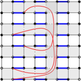
Figure 4. A single cell $B_{x}$, with the reference configuration $M_{0}$ (thick, blue edges). The non-planar edges (red) are drawn in a way that they do not intersect the edges of $M_{0}$ and do not exit the cell. Note that non-planar edges can cross each other. The dotted edges, crossed by the planar edges, belong to $P_{N_{L}}$. If the non-planar edges cross only horizontal edges in the same column (shaded) of the cell and vertical edges from every second row (shaded), the graph obtained by removing red edges and dotted edges is $2$-connected.

We start by rewriting

$$Z_{L,\underline{t}}=\sum_{J\subset N_{L}}\sum_{S\subset P_{J}}\sum_{M\in\Omega_{J,S}}w(M)$$ (3.29)

where $\Omega_{J,S}$ is the set of dimer configurations $M$ such that a non-planar edge belongs to $M$ iff it belongs to $J$, and an edge in $P_{J}$ belongs to $M$ iff it belongs to $S$. Given $M\in\Omega_{J,S}$, we write $M$ as the disjoint union $M=J\cup S\cup M^{\prime}$ and, with obvious notations, $w(M)=w(M^{\prime})w(S)w(J)$ so that (3.30) becomes

$$Z_{L,\underline{t}}=\sum_{J\subset N_{L}}w(J)\sum_{S\subset P_{J}}w(S)\sum_{M^{\prime}\sim{J,S}}w(M^{\prime})$$ (3.30)

where $M^{\prime}\sim S,J$ means that $M^{\prime}\cup S\cup J$ is a dimer configuration in $\Omega_{J,S}$. To proceed, we use the following

Lemma 1.

There exists $\epsilon_{S}^{J}=\pm 1$ such that

$$\sum_{M^{\prime}\sim J,S}w(J)w(S)w(M^{\prime})=\epsilon_{S}^{J}\sum_{\theta\in\{-1,+1\}^{2}}\frac{c_{\theta}}{2}\int D\psi\,e^{-\psi^{+}K_{\theta}\psi^{-}}\prod_{e\in J\cup S}\psi(e).$$ (3.31)

Here, $\psi(e),e\in J\cup S$ is the same as $\psi_{\theta}(e)$: we have removed the index $\theta$ because, since the endpoints $b,w$ of $e$ belong to the same cell, the right hand side of (3.28) is independent of $\theta$. If $J=S=\emptyset$, the product of $\psi(e)$ in the right hand side of (3.31) should be interpreted as being equal to $1$. Moreover, $\epsilon_{\emptyset}^{\emptyset}=1$ and, letting $J_{x}$ (resp. $S_{x}$) denote the collection of edges in $J$ (resp. $S$) belonging to the cell $B_{x},x\in\Lambda$, one has

$$\epsilon^{J}_{S}=\prod_{x\in\Lambda}\epsilon^{J_{x}}_{S_{x}}.$$ (3.32)

Let us assume for the moment the validity of Lemma 3.32 and conclude the proof of Proposition 1. Going back to (3.30), we deduce that

$$Z_{L,\underline{t}}=\sum_{\theta}\frac{c_{\theta}}{2}\int D\psi\,e^{-\psi^{+}K_{\theta}\psi^{-}}\prod_{x\in\Lambda}\left[\sum_{J_{x}}\sum_{S_{x}\subset P_{J_{x}}}\epsilon^{J_{x}}_{S_{x}}\prod_{e\in J_{x}\cup S_{x}}\psi(e)\right].$$ (3.33)

The expression in brackets in (3.33) can be written as

$$1+F_{x}(\psi)=e^{V^{(x)}(\psi|_{B_{x}})}$$ (3.34)

where $F_{x}(\psi)$ is a polynomial in the Grassmann fields of the box $B_{x}$, such that $F_{x}(0)=0$ and containing only monomials of even degree, and

$$V^{(x)}(\psi|_{B_{x}})=\sum_{n\geq 1}\frac{(-1)^{n-1}}{n}\left(F_{x}(\psi)\right)^{n}.$$ (3.35)

∎

Proof of Lemma 3.32.

First of all, let us define a $2-$connected graph $G_{J,S}$, embedded on the torus, obtained from $G_{L}$ as follows:

1. the edges belonging to $N_{L}\cup P_{J}$ are removed. At this point, every cell $B_{x}$ contains a certain number (possibly zero) of faces that are not elementary squares, and the graph is still $2$-connected, recall the discussion in the caption of Figure 4.

2. the boundary of every such non-elementary face $\eta$ contains an even number of vertices that are endpoints of edges in $J\cup S$. We connect these vertices pairwise via new edges that do not cross each other, stay within $\eta$ and have endpoints of opposite color. See Figure 5 for a description of a possible procedure. We let $E_{J,S}$ denote the collection of the added edges.

Figure 5. Left drawing: a cell with a collection $J$ of non-diagonal edges (red) and of edges $S\subset P_{J}$ (thick blue edges). The dotted edges are those in $P_{J}\setminus S$. Center drawing: the non-elementary face $\eta$ obtained when the edges in $N_{L}\cup P_{J}$ are removed. Only the endpoints of edges in $J\cup S$ are drawn. Right drawing: a planar, bipartite pairing of the endpoints of $J\cup S$. The edges in $E_{J,S}$ are drawn in orange. A possible algorithm for the choice of the pairing is as follows: choose arbitrarily a pair $(w_{1},b_{1})$ of white/black vertices that are adjacent along the boundary of $\eta$ and pair them. At step $n>1$, choose arbitrarily a pair $(w_{n},b_{n})$ that is adjacent once the vertices $w_{i},b_{i},i<n$ are removed. Note that some of the edges in $E_{J,S}$ may form double edges with the edges of $G^{0}_{L}$ on the boundary of $\eta$ (this is the case for $(b_{1},w_{1})$ and $(b_{3},w_{3})$ in the example in the figure).

The first observation is that the l.h.s. of (3.31) can be written as

$$\Big{(}\prod_{e\in J\cup S}t_{e}\Big{)}\Big{(}\sum_{\begin{subarray}{c}M\in\Omega_{G_{J,S}}:\\ M\supset E_{J,S}\end{subarray}}w(M)\Big{)}\Big{|}_{t_{e}=1,e\in E_{J,S}}$$ (3.36)

where $\Omega_{G_{J,S}}$ is the set of perfect matchings of the graph $G_{J,S}$ and as usual $w(M)$ is the product of the edge weights in $M$. The new edges $E_{J,S}$ are assigned a priori arbitrary weights $\{t_{e}\}_{e\in E_{J,S}}$, to be eventually replaced by $1$, and the partition function on $G_{J,S}$ is called $Z_{G_{J,S}}$.

Let $K^{J,S}_{\theta},\theta\in\{-1,+1\}^{2}$ denote the Kasteleyn matrices corresponding to the four relevant orientations $D_{\theta}$ of $G_{J,S}$, for some choice of the basic orientation on $G_{J,S}$ (recall Definition 1). Since $G_{J,S}$ is embedded on the torus and is $2$-connected, Eq.(3.4) guarantees that the sum in the second parentheses in (3.36) can be rewritten (before setting $t_{e}=1$ for all $e\in E_{J,S}$) as

$$\sum_{\begin{subarray}{c}M\in\Omega_{G_{J,S}}\\ M\supset E_{J,S}\end{subarray}}w(M){=\left(\prod_{e\in E_{J,S}}t_{e}\partial_{t_{e}}\right)Z_{G_{J,S}}}=\frac{1}{2}\sum_{\theta}c_{\theta}\left(\prod_{e\in E_{J,S}}t_{e}\partial_{t_{e}}\right)\det K^{J,S}_{\theta}.$$ (3.37)

In fact, the suitable choice of ordering of vertices mentioned in Remark 3 (and therefore the value of signs $c_{\theta}$) is independent of $J,S$, because the reference configuration $M_{0}$ is independent of $J,S$.

Using the basic properties of Grassmann variables, the r.h.s. of (3.37) equals

$$\frac{1}{2}\sum_{\theta}c_{\theta}\left(\prod_{e\in E_{J,S}}t_{e}\partial_{t_{e}}\right)\int D\psi\,e^{-\psi^{+}K^{J,S}_{\theta}\psi^{-}}\\ =\frac{1}{2}\sum_{\theta}c_{\theta}\int D\psi\,e^{-\psi^{+}K^{J,S}_{\theta}\psi^{-}}\left(\prod_{e\in E_{J,S}}\psi^{J,S}_{\theta}(e)\right)$$ (3.38)

where, in analogy with (3.28), $\psi^{J,S}_{\theta}(e)=-K^{J,S}_{\theta}(b,w)\psi^{+}_{b}\psi^{-}_{w}$. We claim:

Lemma 2.

The choice of the basic orientation of $G_{J,S}$ can be made so that the Kasteleyn matrices $K_{\theta}^{J,S}$ satisfy:

1. if $e=(b,w)\in G_{J,S}\setminus E_{J,S}$, then $K^{J,S}_{\theta}(b,w)=K_{\theta}(b,w)$, with $K_{\theta}$ the Kasteleyn matrices of the graph $G_{L}^{0}$, fixed by the choices explained in Section 3.2.

2. if instead $e=(b,w)\in E_{J,S}$ and is contained in cell $B_{x}$, then $K^{J,S}_{\theta}(b,w)=t_{e}\sigma_{e}^{J_{x},S_{x}}$ with $\sigma_{e}^{J_{x},S_{x}}=\pm 1$ a sign that depends only on $J_{x},S_{x}$.

Assuming Lemma 2, and letting $E_{J_{x},S_{x}}$ denote the subset of edges in $E_{J,S}$ that belong to cell $B_{x}$, we rewrite (3.38) as

$$\frac{1}{2}\sum_{\theta}c_{\theta}\int D\psi\,e^{-\psi^{+}K_{\theta}\psi^{-}}\prod_{x}\prod_{e=(b,w)\in E_{J_{x},S_{x}}}(-t_{e}\sigma_{e}^{J_{x},S_{x}}\psi^{+}_{b}\psi^{-}_{w}),$$ (3.39)

where we could replace $K^{J,S}_{\theta}$ by $K_{\theta}$ at exponent, because

$$\begin{split}&e^{-\psi^{+}K^{J,S}_{\theta}\psi^{-}}\left(\prod_{e\in E_{J,S}}\psi^{J,S}_{\theta}(e)\right)=\Big{(}\prod_{e=(b,w)\in G_{J,S}\setminus E_{J,S}}e^{-\psi^{+}_{b}K^{J,S}_{\theta}(b,w)\psi^{-}_{w}}\Big{)}\left(\prod_{e\in E_{J,S}}\psi^{J,S}_{\theta}(e)\right)\\ &=\Big{(}\prod_{e=(b,w)\in G_{J,S}\setminus E_{J,S}}e^{-\psi^{+}_{b}K_{\theta}(b,w)\psi^{-}_{w}}\Big{)}\left(\prod_{e\in E_{J,S}}\psi^{J,S}_{\theta}(e)\right)=e^{-\psi^{+}K_{\theta}\psi^{-}}\left(\prod_{e\in E_{J,S}}\psi^{J,S}_{\theta}(e)\right),\end{split}$$ (3.40)

thanks to the Grassmann anti-commutation properties and the fact that $K^{J,S}_{\theta}(b,w)=K_{\theta}(b,w)$ for any $(b,w)\in G_{J,S}\setminus E_{J,S}$. Eq.(3.39) can be further rewritten as

$$\frac{\prod_{e\in E_{J,S}}t_{e}}{\prod_{e\in J\cup S}t_{e}}\sum_{\theta}\frac{c_{\theta}}{2}\int D\psi\,e^{-\psi^{+}K_{\theta}\psi^{-}}\prod_{x}\Big{(}\epsilon^{J_{x}}_{S_{x}}\prod_{e\in J_{x}\cup S_{x}}\psi(e)\Big{)},$$ (3.41)

where $\epsilon^{J_{x}}_{S_{x}}$ is a sign, equal to

$$\pi(J_{x},S_{x})\Big{(}\prod_{e\in E_{J_{x},S_{x}}}\sigma_{e}^{J_{x},S_{x}}\Big{)}\Big{(}\prod_{e\in S_{x}}{\rm sign}(K_{\theta}(e))\Big{)},$$ (3.42)

and $\pi(J_{x},S_{x})$ is the sign of the permutation needed to recast $\prod_{(b,w)\in E_{J_{x},S_{x}}}\psi^{+}_{b}\psi^{-}_{w}$ into the form $\prod_{(b,w)\in J_{x}\cup S_{x}}\psi^{+}_{b}\psi^{-}_{w}$; note also that, for $e\in S_{x}$, $K_{\theta}(e)$ is independent of $\theta$. Putting things together, the statement of Lemma 3.32 follows. ∎

Proof of Lemma 2.

Recall that $G_{J,S}$ is a $2$-connected graph, with the same vertex set as $G^{0}_{L}$, and edge set obtained, starting from $E_{L}$, by removing the edges in $N_{L}\cup P_{J}$ and by adding those in $E_{J,S}$. We introduce a sequence of $2$-connected graphs $G^{(n)},n=0,\dots,z=|E_{J,S}|$ embedded on the torus, all with the same vertex set. Label the edges in $E_{J,S}$ as $e_{1},\dots,e_{z}$ (in an arbitrary order). Then, $G^{(0)}$ is the graph $G_{L}^{0}$ with the edges in $N_{L}\cup P_{J}$ removed and $G^{(n)},1\leq n\leq z$ is obtained from $G^{(0)}$ by adding edges $e_{1},\dots,e_{n}$. Note that $G^{(z)}=G_{J,S}$. We will recursively define the basic orientation $D^{(n)}$ of $G^{(n)}$, in such a way that for $n=z$ the properties stated in the Lemma hold for the Kasteleyn matrices $K_{\theta}^{(z)}=K^{J,S}_{\theta}$. The construction of the basic orientation is such that for $n>m$, $D^{(n)}$ restricted to the edges of $G^{(m)}$ is just $D^{(m)}$. That is, at each step $n>1$ we just need to define the orientation of $e_{n}$.

For $n=0$, $G^{(0)}$ is a sub-graph of $G_{L}^{0}$ and we simply define $D^{(0)}$ to be the restriction of $D$ (the basic orientation of $G^{0}_{L}$) to the edges of the basis graph of $G^{(0)}$. Since the orientation of these edges will not be modified in the iterative procedure, point (i) of the Lemma is automatically satisfied. We need to show that $D^{(0)}$ is indeed a basic orientation for $G^{(0)}$, in the sense of Definition 1. In fact, an inner face $\eta$ of the basis graph of $G^{(0)}$ is either an elementary square face (which belongs also to the basis graph of $G_{L}^{0}$), or it is a non-elementary face as in the middle drawing of Fig. 5. In the former case, the fact that the boundary of $\eta$ is clockwise odd is trivial, since its orientation is the same as in the basic orientation of $G_{L}^{0}$. In the latter case, the boundary of $\eta$ is a cycle $\Gamma$ of $\mathbb{Z}^{2}$ that contains no vertices in its interior. The fact that $\Gamma$ is clockwise odd for $D$ then is well-known [35, Sect.V.D].

Assume now that the basic orientation $D^{(n)}$ of $G^{(n)}$ has been defined for $n\geq 0$ and that the choice of orientation of each $e=(b,w)\in E_{J,S}$ that is an edge of $G^{(n)}$ contained in the cell $B_{x}$, has been done in a way that depends on $J,S$ only through $J_{x},S_{x}$. If $n=z$, recalling how Kasteleyn matrices $K_{\theta}$ are defined in terms of the orientations, claim (ii) of the Lemma is proven. Otherwise, we proceed to step $n+1$, that is we define the orientation of $e_{n+1}$ as explained in Figure 6. This choice is unique and, again, depends on $J,S$ only through $J_{x},S_{x}$. The proof of the Lemma is then concluded. ∎

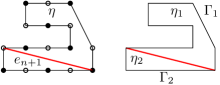
Figure 6. An inner face $\eta$ of $G^{(n)}$ and the edge $e_{n+1}$. After adding $e_{n+1}$, $\eta$ split into two inner faces $\eta_{1},\eta_{2}$ of $G^{(n+1)}$. By assumption, the boundary $\Gamma$ of $\eta$ is clockwise-odd for the orientation $D^{(n)}$. Therefore, exactly one of the two paths $\Gamma_{1},\Gamma_{2}$ contains an odd number of anti-clockwise oriented edges and there is a unique orientation of $e_{n+1}$ such that the boundaries of both $\eta_{1},\eta_{2}$ are clockwise odd. Since, by induction, the orientation of $\Gamma$ depends on $J,S$ only through $J_{x},S_{x}$, with $x$ the label of the cell the face belongs to, the same is true also for the orientation of $e_{n+1}$.

3.4. Generating function and Ward Identities

In this subsection we consider again dimer weights that are periodic under translations by integer multiples of ${\bf e_{1},\bf e_{2}}$.

In view of Proposition 1, the generating function $W_{L}(A)$ of dimer correlations, defined, for $A:E_{L}\rightarrow\mathbb{R}$, by

$$e^{W_{L}(A)}:=\sum_{M\in\Omega_{L}}w(M)\prod_{e\in E_{L}}e^{A_{e}\mathds{1}_{e}(M)},$$ (3.43)

can be equivalently rewritten as $e^{W_{L}(A)}=\frac{1}{2}\sum_{\theta\in\{1,-1\}^{2}}c_{\theta}e^{\mathcal{W}^{(\theta)}_{L}(A)}$, where

$$e^{\mathcal{W}^{(\theta)}_{L}(A)}=\int D\psi e^{S_{\theta}(\psi)+V(\psi,A)},$$ (3.44)

where $S_{\theta}(\psi)=-\psi^{+}K_{\theta}\psi^{-}$ and $V(\psi,A):=-\psi^{+}K_{\theta}^{A}\psi_{-}-S_{\theta}(\psi)+V_{\underline{t}(A)}(\psi)$. Here, $K_{\theta}^{A}$ (resp. $V_{\underline{t}(A)}(\psi)$) is the Kasteleyn matrix as in Section 3.2 (resp. the potential as in (3.27)) with edge weights $\underline{t}(A)=\{t_{e}e^{A_{e}}\}_{e\in E_{L}}$.

As in [28, Sect.3.2], it is convenient to introduce a generalization of the generating function, in the presence of an external Grassmann field coupled with $\psi$. Namely, letting $\phi=\{\phi^{\pm}_{\bf x}\}_{{\bf x}\in{\bf\Lambda}}$ a new set of Grassmann variables, we define

$$\begin{split}&e^{W_{L}(A,\phi)}:=\frac{1}{2}\sum_{\theta\in\{1,-1\}^{2}}c_{\theta}e^{\mathcal{W}^{(\theta)}_{L}(A,\phi)},\\ \text{with}\qquad&e^{\mathcal{W}^{(\theta)}_{L}(A,\phi)}:=\int D\psi\,e^{S_{\theta}(\psi)+V(\psi,A)+(\psi,\phi)}\end{split}$$ (3.45)

and $(\psi,\phi):=\sum_{{\bf x}\in{\bf\Lambda}}(\psi^{+}_{{\bf x}}\phi^{-}_{\bf x}+\phi^{+}_{\bf x}\psi^{-}_{\bf x})$. The generating function is invariant under a local gauge symmetry, which is associated with the local conservation law of the number of incident dimers at each vertex of $\Lambda$:

Proposition 2 (Chiral gauge symmetry).

Given two functions $\alpha^{+}:{\bf\Lambda}\rightarrow\mathbb{R}$ and $\alpha^{-}:{\bf\Lambda}\rightarrow\mathbb{R}$, we have

$${W}_{L}(A,\phi)=-i\sum_{{\bf x}\in{\bf\Lambda}}(\alpha_{{\bf x}}^{+}+\alpha_{\bf x}^{-})+{W}_{L}(A+i\alpha,\phi e^{i\alpha})$$ (3.46)

where, if $e=(b,w)\in E_{L}$ with ${\bf x}$ and ${\bf y}$ the coordinates of $b$ and $w$, respectively, $(A+i\alpha)_{e}:=A_{e}+i(\alpha^{+}_{\bf x}+\alpha^{-}_{\bf y})$, while $(\phi e^{i\alpha})^{\pm}_{\bf x}:=\phi^{\pm}_{\bf x}e^{i\alpha^{\mp}_{\bf x}}$.

The proof simply consists in performing a change of variables in the Grassmann integral, see [26, Proof of Prop.1].

The gauge symmetry (3.46), in turn, implies exact identities among correlation functions, known as Ward Identities. Given edges $e_{1},\ldots,e_{k}$ and a collection of coordinates ${\bf x_{1}},\ldots,{\bf x_{n}},{\bf y_{1}},\ldots,{\bf y_{n}}$, define the truncated multi-point correlation associated with the generating function $\mathcal{W}_{L}(A,\phi)$:

$$\begin{split}&g_{L}(e_{1},\ldots,e_{k};{\bf x_{1}},\ldots,{\bf x_{n}};{\bf y_{1}},\ldots,{\bf y_{n}})\\ &\quad:=\partial_{A_{e_{1}}}\cdots\partial_{A_{e_{k}}}\partial_{\phi^{-}_{\bf y_{1}}}\cdots\partial_{\phi^{-}_{\bf y_{n}}}\partial_{\phi^{+}_{\bf x_{1}}}\cdots\partial_{\phi^{+}_{\bf x_{n}}}{W}_{L}(A,\phi)\big{|}_{A\equiv 0,\phi\equiv 0}.\end{split}$$ (3.47)

Three cases will play a central role in the following: the interacting propagator $G^{(2)}$, the interacting vertex function $G^{(2,1)}$ and the interacting dimer-dimer correlation $G^{(0,2)}$, which deserve a distinguished notation: letting ${\bf x}=(x,\ell),{\bf y}=(y,\ell^{\prime}),{\bf z}=(z,\ell^{\prime\prime})$, and denoting by $e$ (resp. $e^{\prime}$) the edge with black vertex ${\bf x}=(x,\ell)$ (resp. ${\bf y}=(y,\ell^{\prime})$) and label $j\in\mathcal{J}_{\ell}$ (resp. $j^{\prime}\in\mathcal{J}_{\ell^{\prime}}$), we define

$$\begin{split}&G^{(2)}_{\ell,\ell^{\prime};L}(x,y):=g_{L}(\emptyset;{\bf x};{\bf y})\\ &G^{(2,1)}_{j,\ell,\ell^{\prime},\ell^{\prime\prime};L}({x},{y},{z}):=g_{L}(e;{\bf y};{\bf z})\\ &G^{(0,2)}_{j,j^{\prime},\ell,\ell^{\prime};L}({x,y}):=g_{L}(e,e^{\prime};\emptyset;\emptyset).\end{split}$$ (3.48)

As a byproduct of the analysis of Section 5, the $L\to\infty$ of all multi-point correlations $g_{L}(e_{1},\ldots,e_{k},{\bf x_{1}},\ldots,{\bf x_{n}},{\bf y_{1}},\ldots,{\bf y_{n}})$ exist; we denote the limit simply by dropping the index $L$. Let us define the Fourier transforms of the interacting propagator and interacting vertex function via the following conventions: for $\ell,\ell^{\prime},\ell^{\prime\prime}\in\mathcal{I}$ and $j\in\mathcal{J}_{\ell}$, we let

$$\begin{split}&\hat{G}^{(2)}_{\ell,\ell^{\prime}}(p):=\sum_{x\in\mathbb{Z}^{2}}e^{ipx}G^{(2)}_{\ell,\ell^{\prime}}(x,0)\\ &\hat{G}^{(2,1)}_{j,\ell,\ell^{\prime},\ell^{\prime\prime}}(k,p):=\sum_{x,y\in\mathbb{Z}^{2}}e^{-ipx-ik\cdot y}G^{(2,1)}_{j,\ell,\ell^{\prime},\ell^{\prime\prime}}(x,0,y).\end{split}$$ (3.49)

Proposition 3 (Ward identity).

Given $\ell^{\prime},\ell^{\prime\prime}\in\mathcal{I}$, we have

$$\sum_{\begin{subarray}{c}e\in\mathcal{E}\end{subarray}}\hat{G}^{(2,1)}_{j(e),\ell(e),\ell^{\prime},\ell^{\prime\prime}}(k,p)(e^{-ip\cdot v(e)}-1)=\hat{G}^{(2)}_{\ell^{\prime},\ell^{\prime\prime}}(k+p)-\hat{G}^{(2)}_{\ell^{\prime},\ell^{\prime\prime}}(k)$$ (3.50)

where $\mathcal{E}$ is the set of edges $e=(b(e),w(e))$ having an endpoint in the cell $B_{(0,0)}$ and the other in $B_{(0,-1)}\cup B_{(-1,0)}$. Also, $\ell(e)\in\mathcal{I}$ is the type of $b(e)$, $j(e)\in\mathcal{J}_{\ell(e)}$ is the label associated with the edge $e$, while $v(e)\in\{(0,\pm 1),(\pm 1,0)\}$ is the difference of cell labels of $w(e)$ and $b(e)$, see discussion after (3.19).

Proof.

We start by differentiating both sides of the gauge invariance equation (3.46): fix ${\bf x}=(x,\ell)\in{\bf\Lambda}$, differentiate first with respect to $\alpha^{+}_{\bf x}$ and set $\alpha\equiv 0$:

$$1=\sum_{\begin{subarray}{c}e=(b,w)\in E_{L}\\ {\bf x}(b)={\bf x}\end{subarray}}\partial_{A_{e}}{W}_{L}(A,\phi)+\phi^{-}_{\bf x}\partial_{\phi^{-}_{\bf x}}{W}_{L}(A,\phi)$$ (3.51)

where ${\bf x}(b)=(x(b),\ell(b))$ is the coordinate of the black endpoint $b$ of the edge $e$. The above sum thus contains as many terms as the number of edges incident to the black site of coordinate ${\bf x}$, i.e. as the number of elements in $\mathcal{J}_{\ell(b)}$. Then, differentiate with respect to $\phi^{-}_{\bf z}$ and $\phi^{+}_{\bf y}$ and set $A\equiv\phi\equiv 0$:

$$\sum_{\begin{subarray}{c}e=(b,w)\in E_{L}\\ {\bf x}(b)={\bf x}\end{subarray}}g_{L}(e;{\bf y};{\bf z})+\delta_{{\bf x,z}}g_{L}(\emptyset;{\bf y};{\bf z})=0.$$ (3.52)

Repeating the same procedure but differentiating first with respect to $\alpha^{-}_{\bf x}$ rather than $\alpha^{+}_{\bf x}$, we obtain

$$\sum_{\begin{subarray}{c}e=(b,w)\in E_{L}\\ {\bf x}(w)={\bf x}\end{subarray}}g_{L}(e;{\bf y};{\bf z})+\delta_{{\bf x,y}}g_{L}(\emptyset;{\bf y};{\bf z})=0$$ (3.53)

where ${\bf x}(w)$ is the coordinate of the white vertex of $e$. Now we sum both (3.53) and (3.52) over $\ell\in\mathcal{I}$ (the type of the vertex ${\bf x}$) with the cell index $x$ fixed; then we take the difference of the two expressions thus obtained and we send $L\to\infty$. When taking the difference, the contribution from edges whose endpoints both belong to cell $B_{x}$ cancel and we are left with

$$\sum_{e=(x^{\prime},j,\ell)\in E_{\partial B_{x}}}(-1)^{\delta_{x,x^{\prime}}}G^{(2,1)}_{j,\ell,\ell^{\prime},\ell^{\prime}}(x^{\prime},y,z)=(\delta_{x,z}-\delta_{x,y})G^{(2)}_{\ell^{\prime},\ell^{\prime\prime}}(y,z),$$ (3.54)

where we used the notation in (3.48), and we denoted by $E_{\partial B_{x}}$ the set of edges of $E^{0}$ having exactly one endpoint in the cell $B_{x}$. Note that in the first sum, in writing $e=(x^{\prime},j,\ell)$, we used the usual labeling of the edge $e$ in terms of the coordinates $(x^{\prime},\ell)$ of its black site and of the label $j\in\mathcal{J}_{\ell}$. Note also that, if $e=(x^{\prime},j,\ell)\in E_{\partial B_{x}}$, then $x^{\prime}$ is either $x$ or $x\pm(0,1),x\pm(1,0)$. See Figure 7.

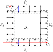
Figure 7. The cell $B_{x}$ (only vertices on its boundary are drawn) together with the edges in $E_{\partial B_{x}}=\mathcal{E}_{1,x}\cup\mathcal{E}_{2,x}\cup\mathcal{E}^{\prime}_{1,x}\cup\mathcal{E}^{\prime}_{2,x}$. To each edge $e$ in $\mathcal{E}_{1,x}$ (resp. in $\mathcal{E}_{2,x}$) there corresponds a unique edge $e^{\prime}$ in $\mathcal{E}_{1,x}^{\prime}$ (resp. $\mathcal{E}_{2,x}^{\prime}$) whose endpoints are of the same type.

Using the last remark in the caption of Fig.7, we can rewrite the sum in the left hand side of (3.54) as a sum over edges in $\mathcal{E}_{1,x}\cup\mathcal{E}_{2,x}$, each term containing the difference of two vertex functions $G^{(2,1)}_{j,\ell,\ell^{\prime},\ell^{\prime\prime}}$. Passing to Fourier space via (3.49), we obtain (3.50), as desired. ∎

Remark 4.

For later reference, note that, if $e$ crosses the path $C_{1}$ (resp. $C_{2}$) of Figure 7, i.e., if $e\in\mathcal{E}_{1,x}$ (resp. $e\in\mathcal{E}_{2,x}$), then, for any $p=(p_{1},p_{2})\in\mathbb{R}^{2}$ and $v(e)$ defined as in the statement of Proposition 3,

$$p\cdot v(e)=\begin{cases}-p_{2}\sigma_{e}&\text{ if $e$ crosses $C_{1}$}\\ +p_{1}\sigma_{e}&\text{ if $e$ crosses $C_{2}$},\end{cases}$$ (3.55)

with $\sigma_{e}=\pm 1$ the same sign appearing in the definition (2.4) of height function.

4. Proof of Theorem 2

One important conclusion of the previous section is Proposition 3, which states the validity of exact identities among the (thermodynamic limit of) correlation functions of the dimer model. In this section we combine these exact identities with a result on the large-distance asymptotics of the correlation functions, which includes the statement of Theorem 1, and use them to prove Theorem 2. The required fine asymptotics of the correlation functions is summarized in the following proposition, whose proof is discussed in Section 5.

Proposition 4.

There exists $\lambda_{0}>0$ such that, for $|\lambda|\leq\lambda_{0}$, the interacting dimer-dimer correlation for $x\neq y$ can be represented in the following form:

$$G^{(0,2)}_{j,j^{\prime},\ell,\ell^{\prime}}(x,y)=\frac{1}{4\pi^{2}Z^{2}(1-\tau^{2})}\sum_{\omega=\pm}\frac{K^{(1)}_{\omega,j,\ell}K^{(1)}_{\omega,j^{\prime},\ell^{\prime}}}{(\phi_{\omega}(x-y))^{2}}$$ (4.1)

$$\qquad+\frac{B}{4\pi^{2}}\sum_{\omega=\pm}\frac{K^{(2)}_{\omega,j,\ell}K^{(2)}_{-\omega,j^{\prime},\ell^{\prime}}}{|\phi_{\omega}(x-y)|^{2(1-\tau)/(1+\tau)}}e^{2i\,p^{\omega}\cdot(x-y)}+R_{j,j^{\prime},\ell,\ell^{\prime}}(x,y)\;,$$

where: $\lambda\mapsto Z$, $\lambda\mapsto\tau$ and $\lambda\mapsto B$ are real-valued analytic functions satisfying $Z=1+O(\lambda)$, $\tau=O(\lambda)$ and $B=1+O(\lambda)$; $\phi_{\omega}(x):=\omega(\beta_{\omega}x_{1}-\alpha_{\omega}x_{2})$ where $\lambda\mapsto\alpha_{\omega},\lambda\mapsto\beta_{\omega}$ are complex-valued analytic functions satisfying $\overline{\alpha_{+}}=-\alpha_{-},\overline{\beta_{+}}=-\beta_{-}$; $\lambda\mapsto K^{(i)}_{\omega,j,\ell}$ with $i\in\{1,2\}$ are complex-valued analytic functions of $\lambda$ satisfying $K^{(i)}_{+,j,\ell}=\overline{K^{(i)}_{-,j,\ell}}$; $\lambda\mapsto p^{\omega}$ are analytic functions with values in $[-\pi,\pi]^{2}$ for $\lambda$ real, satisfying $p^{+}=-p^{-}$ and $2p^{+}\neq 0$ mod $(2\pi,2\pi)$; the correction term $R_{j,j^{\prime},\ell,\ell^{\prime}}(x,y)$ is translational invariant and satisfies $|R_{j,j^{\prime},\ell,\ell^{\prime}}(x,0)|\leq C|x|^{-1+C|\lambda|}$ for some $C>0$.

Moreover, there exists an additional set of complex-valued analytic function $\lambda\mapsto I_{\omega,\ell,\ell^{\prime}},\omega=\pm 1,\ell,\ell^{\prime}\in\mathcal{I},$ such that the Fourier transforms of the interacting propagator and of the interacting vertex function satisfy:

$$\hat{G}^{(2)}_{\ell,\ell^{\prime}}(k+p^{\omega})\stackrel{{\scriptstyle k\to 0}}{{=}}I_{\omega,\ell,\ell^{\prime}}\hat{G}^{(2)}_{R,\omega}(k)[1+O(|k|^{1/2})],$$ (4.2)

and, if $0<\mathfrak{c}\leq|p|,|k|,|k+p|\leq 2\mathfrak{c}$,

$$\hat{G}^{(2,1)}_{j,\ell,\ell^{\prime},\ell^{\prime\prime}}(k+p^{\omega},p)\stackrel{{\scriptstyle\mathfrak{c}\to 0}}{{=}}-\sum_{\omega^{\prime}=\pm}K^{(1)}_{\omega^{\prime},j,\ell}I_{\omega,\ell^{\prime},\ell^{\prime\prime}}\hat{G}^{(2,1)}_{R,\omega^{\prime},\omega}(k,p)[1+O(\mathfrak{c}^{1/2})]\;,$$ (4.3)

where $K^{(1)}_{\omega,j,\ell}$ is the same as in (4.1) and $\hat{G}^{(2)}_{R,\omega}(k)$,$\hat{G}^{(2,1)}_{R,\omega,\omega^{\prime}}(k,p)$ are two functions satisfying, for $D_{\omega}(p)=\alpha_{\omega}p_{1}+\beta_{\omega}p_{2}$,

$$\sum_{\omega^{\prime}=\pm}D_{\omega^{\prime}}(p)\hat{G}^{(2,1)}_{R,\omega^{\prime},\omega}(k,p)=\frac{1}{Z(1-\tau)}\Big{[}\hat{G}^{(2)}_{R,\omega}(k)-\hat{G}^{(2)}_{R,\omega}(k+p)\Big{]}\Big{(}1+O(\lambda|p|)\Big{)}\;,$$ (4.4)

with $Z,\tau$ the same as in (4.1), and

$$\hat{G}^{(2,1)}_{R,-\omega,\omega}(k,p)=\tau\frac{D_{\omega}(p)}{D_{-\omega}(p)}\hat{G}^{(2,1)}_{R,\omega,\omega}(k,p)\Big{(}1+O(|p|)\Big{)}.$$ (4.5)

Finally, $\hat{G}^{(2)}_{R,\omega}(k)\sim c_{1}|k|^{-1+O(\lambda^{2})}$ as $k\to 0$, and, if $0<\mathfrak{c}\leq|p|,|k|,|k+p|\leq 2\mathfrak{c}$, $\hat{G}^{(2,1)}_{R,\omega,\omega^{\prime}}(k,p)\sim c_{2}\mathfrak{c}^{-2+O(\lambda^{2})}$ as $\mathfrak{c}\to 0$, for two suitable non-zero constants $c_{1},c_{2}$.

A few comments are in order. First of all, the statement of Theorem 1, (2.2), follows from (4.1), which is just a way to rewrite it: it is enough to identify $K_{\omega,j,\ell}$ with $(2\pi Z\sqrt{1-\tau^{2}})^{-1}K^{(1)}_{\omega,j,\ell}$, $H_{\omega,j,\ell}$ with $(\sqrt{B}/2\pi)K^{(2)}_{\omega,j,\ell}$, and $\nu$ with $(1-\tau)/(1+\tau)$.

Moreover, we emphasize that Proposition 4 is the analogue of [28, Prop.2] and its proof, discussed in the next section, is a generalization of the corresponding one. The main ideas behind the proof remain the same: in order to evaluate the correlation functions of the non-planar dimer model we start from the Grassmann representation of the generating function, (3.45), and we compute it via an iterative integration procedure, in which we first integrate out the degrees of freedom associated with a length scale $1$, i.e., the scale of the lattice, then those on length scales $2,4,\ldots,2^{-h},\ldots$, with $h<0$. The output of the integration of the first $|h|$ steps of this iterative procedure can be written as a Grassmann integral similar to the original one, with the important difference that the ‘bare potential’ $V(\psi,A)+(\psi,\phi)$ is replaced by an effective one, $V^{(h)}(\psi,A,\phi)$, that, after appropriate rescaling, converges to a non-trivial infrared fixed point as $h\to-\infty$. The large-distance asymptotics of the correlation functions of the dimer model can thus be computed in terms of those of such an infrared fixed-point theory, or of those of any other model with the same fixed point (i.e., of any other model in the same universality class, the Luttinger universality class). The reference model we choose for this asymptotic comparison is described in [28, Section 4], which we refer the reader to for additional details. It is very similar to the Luttinger model, and differs from it just for the choice of the quartic interaction: it describes a system of Euclidean chiral fermions in $\mathbb{R}^{2}$ (modeled by Grassmann fields denoted $\psi^{\pm}_{x,\omega}$, with $x\in\mathbb{R}^{2}$ the space label and $\omega\in\{+,-\}$ the chirality label), with relativistic propagator and a non-local (in both space dimensions, contrary to the case of the Luttinger model) density-density interaction. The bare parameters of the reference model, in particular the strength of its density-density interaction, are chosen in such a way that its infrared fixed point coincides with the one of our dimer model of interest. The remarkable feature of the reference model is that, contrary to our dimer model, it is exactly solvable in a very strong sense: its correlation functions can all be computed in closed form. For our purposes, the relevant correlations are those denoted $G^{(2,1)}_{R,\omega,\omega^{\prime}}$ (the vertex function of the reference model, corresponding to the correlation of the density of chirality $\omega$ with a pair of Grassmann fields of chirality $\omega^{\prime}$), $G^{(2)}_{R,\omega}$ (the interacting propagator, corresponding to the correlation between two Grassmann fields of chirality $\omega$), $S^{(1,1)}_{R,\omega,\omega}$ (the density-density correlation between two densities with the same chirality $\omega$) and $S^{(2,2)}_{R,\omega,-\omega}$ (the mass-mass correlation between two masses – see footnote 8 – of opposite chiralities): these are the correlations, in terms of which the asymptotics of the vertex function, interacting propagator and dimer-dimer correlation of our dimer model can be expressed.

Remark 5.

The connection between the interacting propagator of the dimer model and that of the reference model can be read from (4.2); similarly, the one between the vertex functions of the two models can be read from (4.3). Moreover, in view of the asymptotics of $S^{(1,1)}_{R,\omega,\omega}$ and of $S^{(2,2)}_{R,\omega,-\omega}$, see [28, Eqs.(4.17) and (4.19)], (4.1) can be rewritten as

$$\sum_{\omega=\pm}\big{[}K^{(1)}_{\omega,j,\ell}K^{(1)}_{\omega,j^{\prime},\ell^{\prime}}S^{(1,1)}_{R,\omega,\omega}(x,y)+K^{(2)}_{\omega,j,\ell}K^{(2)}_{-\omega,j^{\prime},\ell^{\prime}}S^{(2,2)}_{R,\omega,-\omega}(x,y)e^{2ip^{\omega}\cdot(x-y)}\big{]}$$ (4.6)

plus a faster decaying remainder, which explains the connection between the dimer-dimer correlation and the density-density and mass-mass correlations of the reference model.

The fact that the infrared behavior of the dimer model discussed in this paper can be described via the same reference model used for the dimer model in [28] is a priori non-obvious. In fact, the Grassmann representation of our non-planar dimer model involves Grassmann fields labelled by $x\in\Lambda$ and $\ell\in\mathcal{I}=\{1,\ldots,m^{2}/2\}$: therefore, one could expect that the infrared behavior of the system is described in terms of a reference model involving fields labelled by an index $\ell\in\mathcal{I}$. This, a priori, could completely change at a qualitative level the nature of the infrared behavior of the system, which crucially depends on the number of mutually interacting massless fermionic fields. For instance, it is well known that 2D chiral fermions with an additional spin degree of freedom (which is the case of interest for describing the infrared behavior of the 1D Hubbard model), behaves differently, depending on the sign of the density-density interaction: for repulsive interactions it behaves qualitatively in the same way as the Luttinger model [8], while for attractive interaction the model dynamically generates a mass and enters a ‘Mott-insulator’ phase [41]. In our setting, remarkably, despite the fact that the number of Grassmann fields used to effectively describe the model is large for a large elementary cell (and, in particular, is always larger than 1), the number of massless fields is the same as in the case of [28]: in fact, out of the $m^{2}/2$ fields $\psi^{\pm}_{(x,\ell)}$ with $\ell\in\{1,\ldots,m^{2}/2\}$, all but one of them are massive, i.e., their correlations decay exponentially to zero at large distances, with rate proportional to the inverse lattice scaling (this is a direct consequence of the fact that, as proven in [38], the characteristic polynomial $\mu$ has only two zeros). Therefore, for the purpose of computing the generating function, we can integrate out the massive fields in one single step of the iterative integration procedure, after which we are left with an effective theory of a single massless Grassmann field with chirality index $\omega$ associated with the two zeros of $\mu$, see (3.9), completely analogous to the one studied in [28, Section 6]. See the next section for details.

While the proof of the fine asymptotic result summarized in Proposition 4 is hard, and based on the sophisticated procedure just described, the proof of Theorem 2 given Proposition 4 is relatively easy, and close to the analogous proof discussed in [28, Section 5]. We provide it here. Let us start with one definition. Given the face $\eta_{0}\in\bar{F}$ ($\bar{F}$ and $\eta_{x},x=(x_{1},x_{2})$ were defined in Section 2.2, just before Theorem 2), let $\mathcal{E}_{1,0}$ (resp. $\mathcal{E}_{2,0}$), be the set of vertical (resp. horizontal) edges crossed by the horizontal (resp. vertical) path $C_{\eta_{0}\to\eta^{\prime}}$ connecting $\eta_{0}$ to the face $\eta^{\prime}\in\bar{F}$ given by $\eta^{\prime}=\eta_{(1,0)}$ (resp. $\eta^{\prime}=\eta_{(0,1)}$). See Fig.7, where the same paths and edge sets around the cell $B_{x}$ rather than $B_{0}$ are shown. For $e\in\mathcal{E}_{q,0}$, $q=1,2$, we let $(x(e),\ell(e))$ denote the coordinates of its black vertex and $j(e)\in\mathcal{J}_{\ell(e)}$ the type of the edge. We also recall from Section 2.2 that $\sigma_{e}=\pm 1$ is defined in (2.4).

Proposition 5.

For $q=1,2$ and $\omega=\pm$, one has

$$\sum_{e\in\mathcal{E}_{q,0}}\sigma_{e}\frac{K^{(1)}_{\omega,j(e),\ell(e)}}{Z\sqrt{1-\tau^{2}}}=-i\omega\sqrt{\nu}\,{\mathrm{d}}_{q}{\phi}_{\omega}$$ (4.7)

where $\nu=(1-\tau)/(1+\tau)$, and

$$\begin{split}&{\mathrm{d}}_{1}\phi_{\omega}:=\phi_{\omega}(x+(1,0)))-\phi_{\omega}(x)=\omega\beta_{\omega},\\ &{\mathrm{d}}_{2}\phi_{\omega}:=\phi_{\omega}(x+(0,1)))-\phi_{\omega}(x)=-\omega\alpha_{\omega}.\end{split}$$ (4.8)

Proof.

Start with the Ward Identity in Fourier space (3.50) evaluated for $k$ replaced by $k+p^{\omega}$ and substitute (4.2) and (4.3) in it for $\mathfrak{c}\to 0$. Recalling that $0<\mathfrak{c}<|k|,|p|,|k+p|<2\mathfrak{c}$ we obtain for $\mathfrak{c}$ small

$$\sum_{\omega^{\prime}=\pm}\mathcal{D}_{\omega^{\prime}}(p)G^{(2,1)}_{R,\omega^{\prime},\omega}(k,p)=(G^{(2)}_{R,\omega}(k)-G^{(2)}_{R,\omega}(k+p))(1+O(\mathfrak{c}^{1/2}))$$ (4.9)

where $\mathcal{D}_{\omega}(p):=-i\sum_{e\in\mathcal{E}}K^{(1)}_{\omega,j(e),\ell(e)}p\cdot v(e)$, with $\mathcal{E}=\mathcal{E}_{1,0}\cup\mathcal{E}_{2,0}$ the set of edges defined in Proposition 3. Now comparing the above relation with the identity (4.4), by using (4.5) and by identifying terms at dominant order for $|p|$ small we obtain (recall the definition of $D_{\omega}(p)$ right before (4.4)):

$$\mathcal{D}_{\omega}(p)D_{-\omega}(p)+\tau\mathcal{D}_{-\omega}(p)D_{\omega}(p)=Z(1-\tau^{2})D_{\omega}(p)D_{-\omega}(p).$$ (4.10)

Letting $p=(p_{1},p_{2}),v(e)=(v_{1}(e),v_{2}(e))$, imposing $p_{2}=0,p_{1}\neq 0$ first and $p_{1}=0,p_{2}\neq 0$ then, we find a linear system for the coefficients $-i\sum_{e\in\mathcal{E}}K_{\omega,\ell(e),j(e)}v_{q}(e)$, for $q=1,2$ and $\omega=\pm$ whose solution is

$$\begin{split}&\sum_{e\in\mathcal{E}}K^{(1)}_{\omega,j(e),\ell(e)}v_{1}(e)=iZ(1-\tau)\alpha_{\omega},\\ &\sum_{e\in\mathcal{E}}K^{(1)}_{\omega,j(e),\ell(e)}v_{2}(e)=iZ(1-\tau)\beta_{\omega}.\end{split}$$ (4.11)

Note that, by the very definition of $\mathcal{E}=\mathcal{E}_{1,0}\cup\mathcal{E}_{2,0}$, if $e\in\mathcal{E}$, then $v_{1}(e)\neq 0$ iff $e\in\mathcal{E}_{2,0}$, while $v_{2}(e)\neq 0$ iff $e\in\mathcal{E}_{1,0}$. Recall also the relation between $v(e)$ and $\sigma_{e}$ outlined in Remark 4: in view of this, (4.11) is equivalent to

$$\sum_{e\in\mathcal{E}_{1,0}}\frac{K^{(1)}_{\omega,j(e),\ell(e)}}{Z\sqrt{1-\tau^{2}}}\sigma_{e}=-i\sqrt{\frac{1-\tau}{1+\tau}}\,\beta_{\omega}=-i\omega\sqrt{\nu}\,{\mathrm{d}}_{1}\phi_{\omega}$$ (4.12)

$$\sum_{e\in\mathcal{E}_{2,0}}\frac{K_{\omega,j(e),\ell(e)}}{Z\sqrt{1-\tau^{2}}}\sigma_{e}=i\sqrt{\frac{1-\tau}{1+\tau}}\,\alpha_{\omega}=-i\omega\sqrt{\nu}\,{\mathrm{d}}_{2}\phi_{\omega},$$ (4.13)

where we used $\nu=(1-\tau)/(1+\tau)$ and the definition (4.8). ∎

Proof of Theorem 2.

Given Proposition 5, the proof of Theorem 2 is essentially identical to that of [28, Eq.(2.47)] and of [25, Proof of (7.26)]. Here we give only a sketch and we emphasize only the role played by the relation (4.7) that we have just proven.

First of all, we choose a path $C_{\eta_{x^{(1)}}\to\eta_{x^{(2)}}}$ from face $\eta_{x^{(1)}}$ to $\eta_{x^{(2)}}$ that crosses only edges that join different cells. Since $\eta_{x^{(1)}},\eta_{x^{(2)}}\in\bar{F}$, the path $C_{\eta_{x^{(1)}}\to\eta_{x^{(2)}}}$ visits a sequence of faces $\eta_{y^{(1)}},\dots,\eta_{y^{(k)}}\in\bar{F}$, with $y^{(1)}={x^{(1)}},y^{(k)}={x^{(2)}}$ and $|y^{(a)}-y^{(a+1)}|=1$. The set of edges crossed by the path between $\eta_{y^{(a)}}$ and $\eta_{y^{(a+1)}}$, denoted $\mathcal{E}_{(a)}$, is a translation of either $\mathcal{E}_{1,0}$ (if $y^{(a+1)}-y^{(a)}$ is horizontal) or $\mathcal{E}_{2,0}$ (if $y^{(a+1)}-y^{(a)}$ is vertical). Similarly, one defines a path $C_{\eta_{x^{(3)}}\to\eta_{x^{(4)}}}$ and correspondingly a sequence of faces $\eta_{z^{(1)}},\dots,\eta_{z^{(k^{\prime})}}\in\bar{F}$ and $\mathcal{E}^{\prime}_{(a)}$ the set of edges crossed by the path between $\eta_{z^{(a)}}$ and $\eta_{z^{(a+1)}}$. The two paths can be chosen so that $C_{\eta_{x^{(1)}}\to\eta_{x^{(2)}}}$ is of length $O(|x^{(1)}-x^{(2)}|)$ and $C_{\eta_{x^{(3)}}\to\eta_{x^{(4)}}}$ is of length $O(|x^{(3)}-x^{(4)}|)$, while they are at mutual distance at least of order $\min(|x^{(i)}-x^{(j)}|,i\neq j)$. See [25] for more details.

From the definition (2.4) of height function, we see that

$$\mathbb{E}_{\lambda}\left[(h(\eta_{x^{(1)}})-h(\eta_{x^{(2)}}));(h(\eta_{x^{(3)}})-h(\eta_{x^{(4)}}))\right]=\sum_{\begin{subarray}{c}1\leq a<k,\\ 1\leq a^{\prime}<k^{\prime}\end{subarray}}\sum_{\begin{subarray}{c}e\in\mathcal{E}_{(a)},\\ e^{\prime}\in\mathcal{E}^{\prime}_{(a^{\prime})}\end{subarray}}\sigma_{e}\sigma_{e^{\prime}}\mathbb{E}_{\lambda}[{\mathbbm{1}}_{e};{\mathbbm{1}}_{e^{\prime}}].$$ (4.14)

As a consequence of Proposition 4, for edges $e,e^{\prime}$ with black sites of coordinates $(x,\ell),(x^{\prime},\ell^{\prime})$ and with orientations $j,j^{\prime}$, respectively, we have that

$$\begin{split}\mathbb{E}_{\lambda}[{\mathbbm{1}}_{e};{\mathbbm{1}}_{e^{\prime}}]&=\sum_{\omega=\pm}\frac{K^{(1)}_{\omega,j,\ell}}{Z\sqrt{1-\tau^{2}}}\frac{K^{(1)}_{\omega,j^{\prime},\ell^{\prime}}}{Z\sqrt{1-\tau^{2}}}\frac{1}{4\pi^{2}(\phi_{\omega}(x-x^{\prime}))^{2}}\\ &+\frac{B}{4\pi^{2}}\sum_{\omega=\pm}\frac{K^{(2)}_{\omega,j,\ell}K^{(2)}_{-\omega,j^{\prime},\ell^{\prime}}}{|\phi_{\omega}(x-x^{\prime})|^{2(1-\tau)/(1+\tau)}}e^{2ip^{\omega}(x-x^{\prime})}+R_{j,j^{\prime},\ell,\ell^{\prime}}(x,x^{\prime}).\end{split}$$ (4.15)

At this point we plug this expression into (4.14). The oscillating term in (4.15), proportional to $B$, and the error term $R_{j,\ell,j^{\prime},\ell}(x,x^{\prime})$, once summed over $e,e^{\prime}$, altogether end up in the error term in (2.5) (see the analogous argument in [25, Section 3.2 and 7.3]). As for the main term involving $K^{(1)}_{\omega,j,\ell}$, we observe that if we fix $a,a^{\prime}$, then for $e\in\mathcal{E}_{(a)},e^{\prime}\in\mathcal{E}^{\prime}_{(a^{\prime})}$ we can replace in (4.15) $\phi_{\omega}(x-x^{\prime})$ by $\phi_{\omega}(y^{(a)}-z^{(a^{\prime})})$, up to an error term of the same order as $R_{j,j^{\prime},\ell,\ell^{\prime}}(x,x^{\prime})$, which again contributes to the error term in (2.5). We are thus left with

$$\begin{split}&\sum_{\omega=\pm}\sum_{\begin{subarray}{c}1\leq a<k,\\ 1\leq a^{\prime}<k^{\prime}\end{subarray}}\frac{1}{4\pi^{2}(\phi_{\omega}(y^{(a)}-z^{(a^{\prime})}))^{2}}\sum_{e\in\mathcal{E}_{(a)}}\sigma_{e}\frac{K_{\omega,j(e),\ell(e)}}{Z\sqrt{1-\tau^{2}}}\sum_{e^{\prime}\in\mathcal{E}^{\prime}_{(a^{\prime})}}\sigma_{e^{\prime}}\frac{K_{\omega,j(e^{\prime}),\ell(e^{\prime})}}{Z\sqrt{1-\tau^{2}}}\\ &=-\nu\sum_{\omega=\pm}\sum_{\begin{subarray}{c}1\leq a<k,\\ 1\leq a^{\prime}<k^{\prime}\end{subarray}}\frac{(y^{(a+1)}-y^{(a)})\cdot{\rm d}\phi_{\omega}\,(z^{(a^{\prime}+1)}-z^{(a^{\prime})})\cdot{\rm d}\phi_{\omega}}{4\pi^{2}(\phi_{\omega}(y^{(a)}-z^{(a^{\prime})}))^{2}}\\ &=-\frac{\nu}{2\pi^{2}}\Re\Big{[}\sum_{\begin{subarray}{c}1\leq a<k,\\ 1\leq a^{\prime}<k^{\prime}\end{subarray}}\frac{(y^{(a+1)}-y^{(a)})\cdot{\rm d}\phi_{+}\,(z^{(a^{\prime}+1)}-z^{(a^{\prime})})\cdot{\rm d}\phi_{+}}{(\phi_{+}(y^{(a)}-z^{(a^{\prime})}))^{2}}\Big{]}\end{split}$$ (4.16)

where in the first step we used Proposition 5 and defined ${\rm d}\phi_{\omega}:=({\rm d}_{1}\phi_{\omega},{\rm d}_{2}\phi_{\omega})$. As explained in [28, Section 5.2] and [25, Section 7.3] (see also [38, Section 4.4.1] in the non-interacting case), this sum equals the integral in the complex plane

$$-\frac{\nu}{2\pi^{2}}\Re\int_{\phi_{+}(x^{(1)})}^{\phi_{+}(x^{(2)})}dz\int_{\phi_{+}(x^{(3)})}^{\phi_{+}(x^{(4)})}dz^{\prime}\frac{1}{(z-z^{\prime})^{2}}$$ (4.17)

(which equals the main term in the r.h.s. of (2.5)), plus an error term (coming from the Riemann approximation) estimated as in the r.h.s. of (2.5). ∎

5. Proof of Proposition 4

In this section we give the proof of Proposition 4 (which immediately implies Theorem 1, as already commented above), via the strategy sketched after its statement. As explained there, the novelty compared to the proof in [28, Section 6] is the reduction to an effective model involving a single Grassmann critical field $\varphi$, of the same form as the one analyzed in [28, Section 6]. Therefore, most of this section will be devoted to the proof of such reduction, which consists of the following steps. Our starting point is the generating function of correlations in its Grassmann form, see (3.45). In (3.45), we first integrate out the ‘ultraviolet’ degrees of freedom at the lattice scale, see Section 5.1 below; the resulting effective theory can be conveniently formulated in terms of a collection of chiral fields $\{\psi^{\pm}_{x,\omega}\}_{x\in\Lambda}^{\omega\in\{+,-\}}$, where $\psi^{\pm}_{x,\omega}$ are Grassmann vectors with $|\mathcal{I}|$ components, which represent fluctuation fields supported in momentum space close to the unperturbed Fermi points $p_{0}^{\omega}$. Next, we perform a ‘rigid rotation’ of these Grassmann vectors via a matrix $B$ that is independent of $x$ but may depend on the chirality index $\omega$; the rotation is chosen so to block-diagonalize the reference quadratic part of the effective action, in such a way that the corresponding covariance is the direct sum of two terms, a one-dimensional one, which is singular at $p^{\omega}_{0}$, and a non-singular one, of dimension $|\mathcal{I}|-1$; the components associated with this non-singular $(|\mathcal{I}|-1)\times(|\mathcal{I}|-1)$ block are referred to as the ‘massive components’, which can be easily integrated out in one step, see Section 5.2 below (this is the main novel contribution of this section, compared with the multiscale analysis in [28]). In Section 5.3 below we reduce essentially to the setting of [28], that is, to an effective theory that involves one single-component “quasi-particle” chiral massless field, which can be analyzed along the same lines as [28, Section 6]. Finally, in Section 5.4 we conclude the proof of Proposition 4.

5.1. Integration of the ultraviolet degrees of freedom

We intend to compute the generating function (3.45) with $\theta$ boundary conditions. We introduce Grassmann variables in Fourier space via the following transformation:

$$\hat{\psi}^{\pm}_{k}:=\sum_{x\in\Lambda}e^{\mp ikx}\psi^{\pm}_{x},\qquad\psi^{\pm}_{x}=\frac{1}{L^{2}}\sum_{k\in\mathcal{P}(\theta)}e^{\pm ikx}\hat{\psi}^{\pm}_{k},$$ (5.1)

where we recall that each $\psi_{x}^{\pm}$ and each $\hat{\psi}_{k}^{\pm}$ has $|\mathcal{I}|$ components and indeed we assume that $\psi_{x}^{+}=(\psi^{+}_{x,1},\dots,\psi^{+}_{x,|\mathcal{I}|})$ is a row vector while similarly $\psi^{-}_{x}$ is a column vector (whenever unnecessary, we shall drop the ‘color’ index $\ell\in\mathcal{I}$); in this way the transformation above is performed component-wise.

For each $\theta\in\{-1,+1\}^{2}$, we let $p^{\omega}_{\theta}$, $\omega=\pm 1$ denote the element of $\mathcal{P}(\theta)$ that is closest to $p^{\omega}_{0}$, we rewrite

$$\psi^{\pm}_{x}=\psi^{\prime\pm}_{x}+\Psi^{\pm}_{x}$$

with

$$\psi^{\prime\pm}_{x}=\frac{1}{L^{2}}\sum_{k\not\in\{p^{+}_{\theta},p^{-}_{\theta}\}}e^{\pm ikx}\hat{\psi}^{\pm}_{k},\quad\Psi^{\pm}_{x}={\frac{1}{L^{2}}}\sum_{k\in\{p^{+}_{\theta},p^{-}_{\theta}\}}e^{\pm ikx}\hat{\psi}^{\pm}_{k}.$$ (5.2)

Noting that

$$S_{\theta}(\psi)=S_{\theta}(\Psi)+S_{\theta}(\psi^{\prime}):=-\frac{1}{L^{2}}\sum_{k\in\{p^{+}_{\theta},p^{-}_{\theta}\}}\hat{\psi}^{+}_{k}M(k)\hat{\psi}_{k}^{-}-\frac{1}{L^{2}}\sum_{k\not\in\{p^{+}_{\theta},p^{-}_{\theta}\}}\hat{\psi}^{\prime+}_{k}M(k)\hat{\psi}_{k}^{\prime-},$$

we rewrite

$$e^{\mathcal{W}_{L}^{(\theta)}(A,\phi)}=\Big{(}\prod_{k\not\in\{p^{+}_{\theta},p^{-}_{\theta}\}}\mu(k)\Big{)}\int D\Psi\,e^{S_{\theta}(\Psi)}\int P(D\psi^{\prime})\,e^{V(\psi,A)+(\psi,\phi)},$$ (5.3)

where $D\Psi=\prod_{k\in\{p^{+}_{\theta},p^{-}_{\theta}\}}\big{(}L^{2|\mathcal{I}|}D\hat{\Psi}_{k}\big{)}$ and the Grassmann “measure” $D\hat{\Psi}_{k}$ is defined, as usual, so that

$$\int\Big{(}\prod_{k\in\{p^{+}_{\theta},p^{-}_{\theta}\}}D\hat{\Psi}_{k}\Big{)}\,\Big{(}\prod_{k\in\{p^{+}_{\theta},p^{-}_{\theta}\}}\prod_{\ell\in\mathcal{I}}\hat{\Psi}^{-}_{k,\ell}\hat{\Psi}^{+}_{k,\ell}\Big{)}=1,$$

while we have $\int\Big{(}\prod_{k\in I}D\hat{\Psi}_{k}\Big{)}Q(\Psi)=0$ whenever $Q(\Psi)$ is a monomial in $\{\hat{\Psi}^{\pm}_{k,\ell}\}_{k\in\{p^{+}_{\theta},p^{-}_{\theta}\},\ell\in\mathcal{I}}$ of degree strictly lower or strictly larger than $4|\mathcal{I}|$. Moreover, $P(D\psi^{\prime})$ is the Grassmann Gaussian integration, normalized so that $\int P(D\psi^{\prime})=1$, associated with the propagator

$$g^{\prime}(x,y)=\int P(D\psi^{\prime})\psi^{\prime-}_{x}\psi^{\prime+}_{y}=L^{-2}\sum_{k\not\in\{p^{+}_{\theta},p^{-}_{\theta}\}}e^{-ik(x-y)}(M(k))^{-1}.$$ (5.4)

Note that, since $\psi^{\prime\pm}_{x}$ is a vector with $|\mathcal{I}|$ components, $g^{\prime}(x,y)$ is an $|\mathcal{I}|\times|\mathcal{I}|$ matrix, for fixed $x,y$.

Remark 6.

We emphasize also that, since the zeros of $\mu$ are simple, $\mu(k)\neq 0$ for every $k\not\in\{p^{+}_{\theta},p^{-}_{\theta}\}$ (this is the reason why we singled out the two momenta $p^{\omega}_{\theta}$ where $\mu$ possibly vanishes and $M$ is not invertible).

Next we introduce the following

Definition 2.

We let $\chi_{\omega}:\mathbb{R}^{2}\longrightarrow[0,1],\omega=\pm 1$ be two $C^{\infty}$ functions in the Gevrey class of order 2, see [25, App.C], with the properties that:

1. $\chi_{\omega}(k)=\chi_{-\omega}(-k)$,

2. $\chi_{\omega}(k)=1$ if $|k-p^{\omega}_{0}|\leq c_{0}/2$, and $\chi_{\omega}(k)=1$ if $|k-p^{\omega}_{0}|>c_{0}$, with $c_{0}$ a small enough positive constant, such that in particular the support of $\chi_{+}$ is disjoint from the support of $\chi_{-}$.

We will specify later a more explicit definition of $\chi_{\omega}$. We rewrite $g^{\prime}=g^{(0)}+g^{(1)}$, with

$$\begin{split}&g^{(0)}(x,y)=L^{-2}\sum_{\omega=\pm}\sum_{k\not\in\{p^{+}_{\theta},p^{-}_{\theta}\}}e^{-ik(x-y)}\chi_{\omega}(k)(M(k))^{-1},\\ &g^{(1)}(x,y)=L^{-2}\sum_{k\in\mathcal{P}(\theta)}e^{-ik(x-y)}(1-\chi_{+}(k)-\chi_{-}(k))(M(k))^{-1}.\end{split}$$ (5.5)

Since the cutoff functions $\chi_{\omega}$ are Gevrey functions of order 2, the propagator $g^{(1)}$ has stretched-exponential decay at large distances

$$\|g^{(1)}(x,y)\|\leq Ce^{-\kappa\sqrt{|x-y|}},$$ (5.6)

for suitable $L$-independent constants $C,\kappa>0$, cf. with [28, Eq. (6.21)] $|\mathcal{I}|\times|\mathcal{I}|$ (recall that the propagators are $|\mathcal{I}|\times|\mathcal{I}|$ matrices; the norm in the l.h.s. is any matrix norm). In (5.6), $|x-y|$ denotes the graph distance between $x$ and $y$ on $G_{L}$.

Using the addition principle for Grassmann Gaussian integrations [25, Proposition 1], we rewrite (5.3) as

$$e^{\mathcal{W}_{L}^{(\theta)}(A,\phi)}=\Big{(}\prod_{k\not\in\{p^{+}_{\theta},p^{-}_{\theta}\}}\mu(k)\Big{)}\int D\Psi\,e^{S_{\theta}(\Psi)}\int P_{(0)}(D\psi^{(0)})\\ \times\int P_{(1)}(D\psi^{(1)})\,e^{V(\Psi+\psi^{(0)}+\psi^{(1)},A)+(\Psi+\psi^{(0)}+\psi^{(1)},\phi)}\\ =\Big{(}\prod_{k\not\in\{p^{+}_{\theta},p^{-}_{\theta}\}}\mu(k)\Big{)}e^{L^{2}E^{(0)}+S^{(0)}(J,\phi)}\int D\Psi\,e^{S_{\theta}(\Psi)}\int P_{(0)}(D\psi^{(0)})\,e^{V^{(0)}(\Psi+\psi^{(0)},J,\phi)}$$ (5.7)

where: $P_{(0)}$ and $P_{(1)}$ are the Grassmann Gaussian integrations with propagators $g^{(0)}$ and $g^{(1)}$, respectively, i.e., letting $O_{\omega}=\{k\in\mathcal{P}(\theta)\setminus\{p^{+}_{\theta},p^{-}_{\theta}\}:\chi_{\omega}(k)\neq 0$,

$$P_{(0)}(D\psi)=\prod_{\omega}\frac{\Big{(}L^{2|\mathcal{I}||O_{\omega}|}\prod_{k\in O_{\omega}}D\hat{\psi}_{k}\Big{)}\exp{\Big{(}-L^{-2}\sum_{k\in O_{\omega}}(\chi_{\omega}(k))^{-1}\hat{\psi}^{+}_{k}M(k)\hat{\psi}^{-}_{k}}\Big{)}}{\Big{(}\prod_{k\in O_{\omega}}\mu(k)(\chi_{\omega}(k))^{-|\mathcal{I}|}\Big{)}},$$ (5.8)

and a similar explicit expression for $P_{(1)}$ holds; $J=\{J_{e}\}_{e\in E_{L}}$ with $J_{e}=e^{A_{e}}-1$; $E^{(0)}$, $S^{(0)}$ and $V^{(0)}$ are defined via

$$L^{2}E^{(0)}+S^{(0)}(J,\phi)+V^{(0)}(\psi,J,\phi)=\log\int P_{(1)}(D\psi^{(1)})e^{V(\psi+\psi^{(1)},A)+(\psi+\psi^{(1)},\phi)},$$ (5.9)

with $E^{(0)},S^{(0)}$ fixed uniquely by the condition that $V^{(0)}(0,J,\phi)=S^{(0)}(0,0)=0$. Proceeding as in the proof of [28, Eq.(6.24)], one finds that the effective potential $V^{(0)}$ can be represented as follows:

$$V^{(0)}(\psi,J,\phi)=\sum_{\begin{subarray}{c}n>0\\ m,q\geq 0\\ n+q\in 2\mathbb{N}\end{subarray}}\sum^{*}_{\begin{subarray}{c}\underline{x},\underline{y},\underline{z}\\ \underline{\ell},\underline{\ell}^{\prime},\underline{\ell}^{\prime},\\ \underline{s},\underline{\sigma},\underline{\sigma}^{\prime}\end{subarray}}\psi^{\underline{\sigma}}_{\underline{x},\underline{\ell}}J_{\underline{y},\underline{\ell}^{\prime},\underline{s}}\phi^{\underline{\sigma}^{\prime}}_{\underline{z},\underline{\ell}^{\prime\prime}}W_{n,m,q;\boldsymbol{a}}(\underline{x},\underline{y},\underline{z})$$ (5.10)

where the second sum runs over $\underline{x}\in\Lambda^{n},\underline{y}\in\Lambda^{m},\underline{z}\in\Lambda^{q}$, $\underline{\ell}\in\mathcal{I}^{n},\underline{\ell}^{\prime}\in\mathcal{I}^{m},\underline{\ell}^{\prime\prime}\in\mathcal{I}^{q}$, $\underline{s}\in\mathcal{J}_{\ell_{1}}\times\dots\times\mathcal{J}_{\ell_{m}}$, $\underline{\sigma}\in\{+,-\}^{n},\underline{\sigma}^{\prime}\in\{+,-\}^{q}$ (the $*$ on the sum indicates the constraint that $\sum_{i=1}^{n}\sigma_{i}+\sum_{i=1}^{q}\sigma_{i}^{\prime}=0$), and we defined $J_{\underline{y},\underline{\ell^{\prime}},\underline{s}}:=\prod_{i=1}^{m}J_{y_{i},\ell^{\prime}_{i},s_{i}}$ (here $J_{y,\ell,s}$ stands for $J_{e}$ when the edge $e\in E_{L}$ has black site of coordinates $(y,\ell)$ and orientation $s\in\mathcal{J}_{\ell}$), $\psi^{\underline{\sigma}}_{\underline{x},\underline{\ell}}:=\prod_{i=1}^{n}\psi^{\sigma_{i}}_{x_{i},\ell_{i}}$, and similarly for $\phi^{\underline{\sigma}^{\prime}}_{\underline{z},\underline{\ell}^{\prime\prime}}$; finally, ${\boldsymbol{a}}:=(\underline{\ell},\underline{\sigma},\underline{\ell}^{\prime},\underline{s},\underline{\ell}^{\prime\prime},\underline{\sigma}^{\prime})$. Without loss of generality, we can assume that the kernels $W_{n,m,q;(\underline{\ell},\underline{\sigma},\underline{\ell}^{\prime},\underline{s},\underline{\ell}^{\prime\prime},\underline{\sigma}^{\prime})}$ are symmetric under permutations of the indices $(\underline{y},\underline{\ell}^{\prime},\underline{s})$ and antisymmetric both under permutations of $(\underline{x},\underline{\ell},\underline{\sigma})$ and of $(\underline{z},\underline{\ell}^{\prime\prime},\underline{\sigma}^{\prime})$. A representation similar to (5.10) holds also for $S^{(0)}(J,\varphi)$ with kernels $W^{0,m,q}_{\boldsymbol{a}}(\underline{y},\underline{z})$, where ${\boldsymbol{a}}=(\underline{\ell}^{\prime},\underline{s},\underline{\ell}^{\prime\prime},\underline{\sigma}^{\prime})$. As discussed after [28, Eq.(6.27)], using the Battle-Brydges-Federbush-Kennedy determinant formula and the Gram-Hadamard bound [22, Sec. 4.2] one finds that $E^{(0)}$ and the values of the kernels $W_{n,m,q;\boldsymbol{a}}(\underline{x},\underline{y},\underline{z})$ at fixed positions $\underline{x},\underline{y},\underline{z}$ are real analytic functions of the parameter $\lambda$, for $|\lambda|\leq\lambda_{0}$ and $\lambda_{0}$ sufficiently small but independent of $L$. Moreover, in the analyticity domain, $|E^{(0)}|\leq C|\lambda|$, and

$$\|W_{n,m,q}\|_{\kappa,0}\leq C^{n+m+q}|\lambda|^{\mathbbm{1}_{n+q>2}\max\{1,c(n+q)\}}$$ (5.11)

for suitable positive constants $C,c$ independent of $L$. Here the weighted norm $\|\cdot\|_{\kappa,0}$ is defined as

$$\|W_{n,m,q}\|_{\kappa,0}:=L^{-2}\sup_{\boldsymbol{a}}\sum_{\underline{x},\underline{y},\underline{z}}|W_{n,m,q;\boldsymbol{a}}(\underline{x},\underline{y},\underline{z})|e^{\frac{\kappa}{2}\sqrt{\delta(\underline{x},\underline{y},\underline{z})}},$$ (5.12)

where $\kappa>0$ is the same as in (5.6), and $\delta(\cdot)$ denotes the tree distance, that is the length of the shortest tree on the torus connecting points with the given coordinates.

Remark 7.

The kernels of the effective potential $V^{(0)}$, of $S^{(0)}$, as well as the constant $E^{(0)}$, depend on $\theta$, because both the interaction $V(\psi,A)$ in (5.9) and the propagator $g^{(1)}$ involved in the integration do. Both these effects can be thought of as being associated with boundary conditions assigned to the Grassmann fields, periodic in both coordinate directions for $\theta=(-,-)$, anti-periodic in both coordinate directions for $\theta=(+,+)$, and mixed (periodic in one direction and anti-periodic in the other) in the remaining two cases. Therefore, using Poisson summation formula (see e.g. [25, App. A.2], where notations are different), both $g^{(1)}$ and the kernels of $V^{(0)}$ and $S^{(0)}$ can be expressed via an ‘image rule’, analogous to the summation over images in electrostatics, of the following form:

$$g^{(1)}(x,y)=\sum_{n=(n_{1},n_{2})\in\mathbb{Z}^{2}}(-1)^{\frac{\theta_{1}+1}{2}n_{1}+\frac{\theta_{2}+1}{2}n_{2}}g^{(1),\infty}(x-y+nL),$$ (5.13)

where $g^{(1),\infty}(x)=\lim_{L\to\infty}g^{(1)}(x,0)$ (an analogous sum rule holds for the kernels of $V^{(0)}$ and $S^{(0)}$). From this representation, together with the decay bounds mentioned above on $g^{(1)}$ and on the kernels of the effective potential, it readily follows that the dependence upon $\theta$ of these functions is a finite-size effect that is stretched-exponentially small in $L$. Similarly, the dependence upon $\theta$ of $E^{(0)}$ corresponds to a stretched-exponentially small correction as $L\to\infty$ (see also [25, Appendix A.2]). Therefore, all these corrections are irrelevant for the purpose of computing the thermodynamic limit of thermodynamic functions and correlations. For this reason and for ease of notation, here and below we will not indicate the dependence upon $\theta$ explicitly in most of the functions and constants involved in the multiscale construction.

5.2. Integration of the massive degrees of freedom

Using (5.8) in (5.7) and renaming $\Psi+\psi^{(0)}\equiv\psi$, we get

$$e^{\mathcal{W}_{L}^{(\theta)}(A,\phi)}=e^{L^{2}(t^{(0)}+E^{(0)})+S^{(0)}(J,\phi)}\\ \times\int D\psi\,e^{-L^{-2}\sum_{\omega}\sum_{k\in\mathcal{B}_{\omega}}(\chi_{\omega}(k))^{-1}\hat{\psi}^{+}_{k}M(k)\hat{\psi}^{-}_{k}}e^{V^{(0)}(\psi,J,\phi)}$$ (5.14)

where, recalling that $O_{\omega}$ was defined right before (5.8),

$$\mathcal{B}_{\omega}:=O_{\omega}\cup\{p^{\omega}_{\theta}\}=\{k\in\mathcal{P}(\theta):\chi_{\omega}(k)\neq 0\},$$

$D\psi:=\prod_{\omega=\pm}\Big{(}L^{2|\mathcal{I}||\mathcal{B}_{\omega}|}\prod_{k\in\mathcal{B}_{\omega}}D\hat{\psi}_{k}\Big{)}$ and we have set

$$t^{(0)}:=\frac{1}{L^{2}}\sum_{k\in(\cup_{\omega}\mathcal{B}_{\omega})^{c}}\log\mu(k)+\frac{|\mathcal{I}|}{L^{2}}\sum_{\omega}\sum_{k\in O_{\omega}}\log\chi_{\omega}(k).$$

Since $p^{+}_{0}$ is a simple zero of $\mu(k)$, there exists an invertible complex matrix $B_{+}$ such that

$$B_{+}M(p^{+}_{0})B_{+}^{-1}=\begin{pmatrix}0&0\\ 0&A_{+}\end{pmatrix}$$ (5.15)

for an invertible $(|\mathcal{I}|-1)\times(|\mathcal{I}|-1)$ matrix $A_{+}$. Clearly, $B_{+}$ (and, therefore, $A_{+}$) is not defined uniquely; we choose it arbitrarily, in such a way that (5.15) holds, and fix it once and for all. Taking the complex conjugate in the above equation and using the symmetry of $M$, see (3.13), one finds that the same relation holds at $p^{-}_{0}$ with matrices $B_{-}:=\overline{B_{+}}$, $A_{-}:=\overline{A_{+}}$. Let ${\bf M}_{\omega}(k):=B_{\omega}M(k)B_{\omega}^{-1}$, and define the matrices $T_{\omega}(k),W_{\omega}(k),U_{\omega}(k)$ and $V_{\omega}(k)$ of sizes $1\times 1$, $(|\mathcal{I}|-1)\times(|\mathcal{I}|-1)$, $1\times(|\mathcal{I}|-1)$ and $(|\mathcal{I}|-1)\times 1$, respectively, via

$$\begin{pmatrix}T_{\omega}(k)&U_{\omega}(k)\\ V_{\omega}(k)&W_{\omega}(k)\end{pmatrix}:={\bf M}_{\omega}(k).$$ (5.16)

Analyticity of $M(k)$ in $k$ implies, in particular, that $T_{\omega}(k+p^{\omega}_{0})$, $U_{\omega}(k+p_{0})$ and $V_{\omega}(k+p^{\omega}_{0})$ are all $O(k)$ as $k\to 0$, while $W_{\omega}(k+p^{\omega}_{0})=A_{\omega}+O(k)$. Let $\mathcal{B}^{(2)}_{\omega}\supset\mathcal{B}_{\omega}$ be the ball centered at $p_{0}^{\omega}$ with radius $2c_{0}$ , and assume that $c_{0}$ is so small that $\inf_{k\in\mathcal{B}^{(2)}_{\omega}}|\det W_{\omega}(k)|$ is positive. Taking the determinant at both sides of (5.16), letting $\rho_{\omega}:=\det A_{\omega}$, we find that

$$\mu(k)\stackrel{{\scriptstyle k\to p^{\omega}_{0}}}{{=}}\rho_{\omega}T_{\omega}(k)+O((k-p^{\omega}_{0})^{2})$$

so that, recalling (3.11),

$$T_{\omega}(k+p^{\omega}_{0})\stackrel{{\scriptstyle k\to 0}}{{=}}\frac{\alpha^{0}_{\omega}k_{1}+\beta^{0}_{\omega}k_{2}}{\rho_{\omega}}+O(k^{2}).$$ (5.17)

Since $W_{\omega}(k)$ is non singular on $\mathcal{B}_{\omega}$, for $k\in\mathcal{B}_{\omega}$ we can block diagonalize ${\bf M}_{\omega}$ as

$${\bf M}_{\omega}(k)=\begin{pmatrix}1&U_{\omega}(k)W^{-1}_{\omega}(k)\\ 0&\mathbbm{1}\end{pmatrix}\begin{pmatrix}{\bf T}_{\omega}(k)&0\\ 0&W_{\omega}(k)\end{pmatrix}\begin{pmatrix}1&0\\ W^{-1}_{\omega}(k)V_{\omega}(k)&\mathbbm{1}\end{pmatrix}$$ (5.18)

where ${\bf T}_{\omega}(k):=T_{\omega}(k)-U_{\omega}(k)W^{-1}_{\omega}(k)V_{\omega}(k)$ is the Schur complement of the block $W_{\omega}$. Note that from the properties of $U_{\omega},V_{\omega},W_{\omega}$, the function ${\bf T}_{\omega}$ satisfies

$${\bf T}_{\omega}(k+p^{\omega}_{0})\stackrel{{\scriptstyle k\to 0}}{{=}}\frac{\alpha^{0}_{\omega}k_{1}+\beta^{0}_{\omega}k_{2}}{\rho_{\omega}}+O(k^{2}),$$

like $T_{\omega}$. In view of this decomposition, we perform the following change of Grassmann variables: for $k\in\mathcal{B}_{\omega}$ we define

$$\begin{split}&(\hat{\varphi}^{+}_{k},\hat{\xi}^{+}_{k,1},\dots,\hat{\xi}^{+}_{k,|\mathcal{I}|-1}):=\hat{\psi}^{+}_{k}B_{\omega}^{-1}\begin{pmatrix}1&U_{\omega}(k)W^{-1}_{\omega}(k)\\ 0&\mathbbm{1}\end{pmatrix}\\ &(\hat{\varphi}^{-}_{k},\hat{\xi}^{-}_{k,1},\dots,\hat{\xi}^{-}_{k,|\mathcal{I}|-1})^{T}:=\begin{pmatrix}1&0\\ W^{-1}_{\omega}(k)V_{\omega}(k)&\mathbbm{1}\end{pmatrix}B_{\omega}\hat{\psi}^{-}_{k}.\end{split}$$ (5.19)

For later convenience, we give the following

Lemma 3.

Define $\psi^{\pm}_{x}:=L^{-2}\sum_{\omega}\sum_{k\in\mathcal{B}_{\omega}}e^{\pm ikx}\hat{\psi}^{+}_{k}$ and

$$\xi^{\pm}_{x}(\omega):=L^{-2}\sum_{k\in\mathcal{B}_{\omega}}e^{\pm ikx}\hat{\xi}^{+}_{k},\quad\varphi^{\pm}_{x}(\omega):=L^{-2}\sum_{k\in\mathcal{B}_{\omega}}e^{\pm ikx}\hat{\varphi}^{+}_{k}.$$

Then, the inverse of the transformation (5.19) in $x$ space is

$$\begin{split}&\psi^{+}_{x,\ell}=\sum_{\omega}\Big{(}\varphi^{+}_{x}(\omega)(B_{\omega})_{1\ell}+(\varphi^{+}(\omega)\ast\tau^{+}_{\omega,\ell})_{x}+\sum_{j=2}^{|\mathcal{I}|}\xi^{+}_{x,j-1}(\omega)(B_{\omega})_{j\ell}\Big{)}\\ &\psi^{-}_{x,\ell}=\sum_{\omega}\Big{(}(B_{\omega}^{-1})_{\ell 1}\varphi^{-}_{x}(\omega)+(\tau^{-}_{\omega,\ell}\ast\varphi^{-}(\omega))_{x}+\sum_{j=2}^{|\mathcal{I}|}(B_{\omega}^{-1})_{\ell j}\xi^{-}_{x,j-1}(\omega)\Big{)}\end{split}$$ (5.20)

where

$$\begin{split}&{\tau}_{\omega,\ell}^{+}(x):=-L^{-2}\sum_{k\in\mathcal{P}(\theta)}\sum_{j=2}^{|\mathcal{I}|}e^{ikx}\chi_{\omega}\big{(}\tfrac{k+p_{0}^{\omega}}{2}\big{)}(U_{\omega}(k)\cdot W^{-1}_{\omega}(k))_{j}(B_{\omega})_{j\ell}\\ &{\tau}_{\omega,\ell}^{-}(x):=-L^{-2}\sum_{k\in\mathcal{P}(\theta)}\sum_{j=2}^{|\mathcal{I}|}e^{-ikx}\chi_{\omega}\big{(}\tfrac{k+p_{0}^{\omega}}{2}\big{)}(B^{-1}_{\omega})_{\ell j}(W_{\omega}^{-1}(k)\cdot V_{\omega}(k))_{j}.\end{split}$$ (5.21)

Proof.

The proof is essentially an elementary computation (one inverts the linear relation (5.19) for given $k$ and then takes the Fourier transform to obtain the expression in real space) but there is a slightly delicate point, that is to see where the cut-off function $\chi_{\omega}\big{(}\tfrac{k+p_{0}^{\omega}}{2}\big{)}$ comes from. After a few elementary linear algebra manipulations, one finds that $\psi^{+}_{x,\ell}$ equals an expression like in the r.h.s. of (5.20), where the term $(\varphi^{+}(\omega)\ast\tau^{+}_{\omega,\ell})_{x}$ is replaced by

$$\frac{1}{L^{2}}\sum_{\omega}\sum_{k\in\mathcal{B}_{\omega}}\hat{\varphi}^{+}_{k}f^{\omega}_{\ell}(k)e^{ikx},\quad f^{\omega}_{\ell}(k):=-\sum_{j=2}^{|\mathcal{I}|}\big{(}U_{\omega}(k)W^{-1}_{\omega}(k)\big{)}_{j}(B_{\omega})_{j\ell}.$$

Since the sum is restricted to $k\in\mathcal{B}_{\omega}$, we can freely multiply the summand by $\chi_{\omega}\big{(}\tfrac{k+p_{0}^{\omega}}{2}\big{)}$, which is identically equal $1$ there, since the argument is at distance at most $c_{0}/2$ from $p^{\omega}_{0}$. At that point, we use the fact that

$$\hat{\varphi}^{+}_{k}{\bf 1}_{k\in\mathcal{B}_{\omega}}=\sum_{x}\varphi^{+}_{x}(\omega)e^{-ikx}$$

and we immediately obtain that (5.2) coincides with $(\varphi^{+}(\omega)\ast\tau^{+}_{\omega,\ell})_{x}$, with $\tau^{+}_{\omega,\ell}$ as in (5.21). ∎

At this point we go back to (5.14), that we rewrite as

$$e^{\mathcal{W}_{L}^{(\theta)}(A,\phi)}=e^{L^{2}({\bf t}^{(0)}+E^{(0)})+S^{(0)}(J,\phi)}\\ \times\int D\varphi\,e^{-L^{-2}\sum_{\omega}\sum_{k\in\mathcal{B}_{\omega}}(\chi_{\omega}(k))^{-1}\hat{\varphi}^{+}_{k}{\bf T}_{\omega}(k)\hat{\varphi}^{-}_{k}}\int P_{W}(D\xi)\,e^{\widetilde{V}^{(0)}(\varphi,\xi,J,\phi)}$$ (5.22)

where

$${\bf t}^{(0)}:=L^{-2}\sum_{k\in O^{\prime}}\log\mu(k)+L^{-2}\sum_{\omega=\pm}\sum_{k\in\mathcal{B}_{\omega}}\big{(}\log\det W_{\omega}(k)+\log\chi_{\omega}(k)\big{)},$$

$D\varphi:=\prod_{\omega=\pm}\Big{(}L^{2|\mathcal{B}_{\omega}|}\prod_{k\in\mathcal{B}_{\omega}}D\hat{\varphi}_{k}\Big{)}$, $P_{W}(D\xi)$ is the normalized Gaussian Grassmann integration with propagator (which is a $(|\mathcal{I}|-1)\times(|\mathcal{I}|-1)$ matrix)

$$g^{W}_{\omega,\omega^{\prime}}(x,y):=\int P(D\xi)\,\xi^{-}_{x}(\omega)\xi^{+}_{y}(\omega^{\prime})=\frac{\delta_{\omega,\omega^{\prime}}}{L^{2}}\sum_{k\in P(\theta)}e^{-ik(x-y)}\chi_{\omega}(k)(W_{\omega}(k))^{-1},$$ (5.23)

and $\widetilde{V}^{(0)}(\varphi,\xi,J,\phi)$ is the same as $V^{(0)}(\psi,J,\phi)$, once $\psi$ is re-expressed in terms of the new variables $(\varphi,\xi)$, as in Lemma 3.

Remark 8.

Note that, because of $\chi(\cdot)$, the sums (5.21) defining $\tau^{\pm}_{\omega,\ell}(x)$ are restricted to momenta $k\in\mathcal{B}_{\omega}^{(2)}$ where $W_{\omega}$ is indeed invertible. Note also that, from the smoothness of $\hat{\tau}^{\pm}_{\omega,\ell}(k)$ it follows that $\tau^{\pm}_{\omega,\ell}(x)$ decays to zero in a stretched-exponential way, similar to (5.6). That is, $\psi$ is essentially a local function of $\varphi,\xi$. As a consequence, the kernels of $\widetilde{V}^{(0)}$ satisfy qualitatively the same bounds as those of $V^{(0)}$.

Since $W_{\omega}(\cdot)$ is smooth and invertible in the support of $\chi_{\omega}$, we see from (5.23) that the propagator of the variables $\{\xi_{x}(\omega)\}$ decays as

$$\|g^{W}(x,y)\|\leq Ce^{-\kappa\sqrt{|x-y|}}$$

uniformly in $L$, a behavior analogous to (5.6). For this reason, we call the variables $\{\xi_{x}(\omega)\}$ massive. On the other hand, we call critical the remaining $\{\varphi_{x}(\omega)\}$ variables.

The integration of the massive fields $\xi$, which is performed in a way completely analogous to the one of $\psi^{(1)}$ in (5.9), produces an expression for the generating functional in terms of a Grassmann integral involving only the critical fields $\varphi$:

$$e^{\mathcal{W}_{L}^{(\theta)}(A,\phi)}=e^{L^{2}E^{(-1)}+S^{(-1)}(J,\phi)}\int D\varphi e^{-L^{-2}\sum_{\omega}\sum_{k\in\mathcal{B}_{\omega}}\hat{\varphi}^{+}_{k}(\chi_{\omega}(k))^{-1}{\bf T_{\omega}}(k)\hat{\varphi}^{-}_{k}}e^{V^{(-1)}(\varphi,J,\phi)}$$ (5.24)

where

$$L^{2}(E^{(-1)}-{\bf t}^{(0)}-E^{(0)})+S^{(-1)}(J,\phi)-S^{(0)}(J,\phi)+V^{(-1)}(\varphi,J,\phi)\\ =\log\int P_{W}(D\xi)e^{\widetilde{V}^{(0)}(\varphi,\xi,J,\phi)}$$ (5.25)

and $V^{(-1)},S^{(-1)}$ are fixed in such a way that $V^{(-1)}(0,J,\phi)=S^{(-1)}(0,0)=0$. The effective potential $V^{(-1)}$ can be represented in a way similar to (5.10), namely

$$V^{(-1)}(\varphi,J,\phi)=\sum_{\begin{subarray}{c}n>0\\ m,q\geq 0\\ n+q\in 2\mathbb{N}\end{subarray}}\sum^{*}_{\begin{subarray}{c}\underline{x},\underline{y},\underline{z}\\ \underline{\ell}^{\prime},\underline{\ell}^{\prime\prime},\underline{\omega}\\ \underline{s},\underline{\sigma},\underline{\sigma}^{\prime}\end{subarray}}\varphi^{\underline{\sigma}}_{\underline{x}}(\underline{\omega})J_{\underline{y},\underline{\ell}^{\prime},\underline{s}}\phi^{\underline{\sigma}^{\prime}}_{\underline{z},\underline{\ell}^{\prime\prime}}W^{(-1)}_{n,m,q;\boldsymbol{a}}(\underline{x},\underline{y},\underline{z};\underline{\omega})$$ (5.26)

where $\underline{\omega}\in\{-1,+1\}^{n}$ and $\varphi^{\underline{\sigma}}_{\underline{x}}(\underline{\omega}):=\prod_{i=1}^{n}\varphi^{\sigma_{i}}_{x_{i}}(\omega_{i})$, while the other symbols and labels have the same meaning as in (5.10). In virtue of the decay properties of the propagator $g_{\omega,\omega^{\prime}}^{W}$, the kernels $W^{(-1)}_{n,m,q;\boldsymbol{a}}(\underline{x},\underline{y},\underline{z};\underline{\omega})$ of $V^{(-1)}(\varphi,J,\phi)$ satisfy the same bounds as (5.11).

5.3. Reduction to the setting of [28]

We are left with the integral of the critical variables, which we want to perform in a way analogous to that discussed in [28, Section 6]. In order to get to a point where we can literally apply the results of [28], a couple of extra steps are needed. First, in order to take into account the fact that, in general, the interaction has the effect of changing the location of the singularity in momentum space of the propagator of $\varphi$, as well as the value of the residues at the singularity, we find it convenient to rewrite the ‘Grassmann action’ in (5.24),

$$-L^{-2}\sum_{\omega}\sum_{k\in\mathcal{B}_{\omega}}\hat{\varphi}^{+}_{k}(\chi_{\omega}(k))^{-1}{\bf T_{\omega}}(k)\hat{\varphi}^{-}_{k}+V^{(-1)}(\varphi,J,\phi),$$

in the form of a reference quadratic part, with the ‘right’ singularity structure, plus a remainder, whose specific value will be fixed a posteriori via a fixed-point argument. More precisely, we proceed as described in [28, Section 6.1]: we introduce

$$N(\varphi)=L^{-2}\sum_{\omega}\sum_{k\in\mathcal{B}_{\omega}}\hat{\varphi}^{+}_{k}(-{\bf T_{\omega}}(p^{\omega})+a_{\omega}(k_{1}-p^{\omega}_{1})+b_{\omega}(k_{2}-p^{\omega}_{2}))\hat{\varphi}^{-}_{k}$$ (5.27)

where $p^{\omega},a_{\omega},b_{\omega}$ will be fixed a posteriori, and are assumed to satisfy

$$|p^{\omega}-p^{\omega}_{0}|\ll 1$$ (5.28)

for $\lambda$ small, $p^{+}=-p^{-}$ and $\overline{a_{+}}=-a_{-},\overline{b_{+}}=-b_{-}$. Define also

$$C_{\omega}(k):={\bf T_{\omega}}(k)-\chi_{\omega}(k)\Big{(}{\bf T_{\omega}}(p^{\omega})-a_{\omega}(k_{1}-p^{\omega}_{1})-b_{\omega}(k_{2}-p^{\omega}_{2})\Big{)}$$ (5.29)

and note that it satisfies $C_{\omega}(p^{\omega})=0$,

$$\partial_{k_{1}}C_{\omega}(p^{\omega})=\partial_{k_{1}}{\bf T_{\omega}}(p^{\omega})+a_{\omega}=:\alpha_{\omega},\qquad\partial_{k_{2}}C_{\omega}(p^{\omega})=\partial_{k_{2}}{\bf T_{\omega}}(p^{\omega})+b_{\omega}=:\beta_{\omega},$$ (5.30)

as well as the symmetry $C_{-\omega}(-k)=\overline{C_{\omega}(k)}$.

Let us introduce the matrix $\mathcal{M}$ (the same as in [28, Eq.(4.1)]) given by

$$\mathcal{M}=\frac{1}{\sqrt{\Delta}}\begin{pmatrix}\beta^{1}&\beta^{2}\\ -\alpha^{1}&-\alpha^{2}\end{pmatrix}$$ (5.31)

where $\alpha^{1}$ and $\alpha^{2}$ (resp. $\beta^{1}$ and $\beta^{2}$) are, respectively, the real and imaginary part of $\alpha_{+}$ (resp. $\beta_{+}$), see (5.30), and $\Delta:=\alpha^{1}\beta^{2}-\alpha^{2}\beta^{2}$ is a positive real number, in agreement with (3.16): note, in fact, that at $\lambda=0$ the sign of $\Delta$ is the same as the sign of $\text{Im}(\beta_{+}/\alpha_{+})$. At this point, we can finally fix the cut-off functions $\chi_{\omega}$ of Definition 2 as follows:

$$\chi_{\omega}(k):=\chi(|\mathcal{M}^{-1}(k-p^{\omega})|)$$

where $\chi:\mathbb{R}\mapsto[0,1]$ is a compactly supported function in the Gevrey class of order $2$. It is immediate to verify that $\chi$ can be chosen so that that properties (i)-(ii) of Definition 2 are verified.

Given this, we rewrite (5.24) as

$$e^{\mathcal{W}_{L}^{(\theta)}(A,\phi)}=e^{L^{2}E^{(-1)}+S^{(-1)}(J,\phi)}\int D\varphi e^{-L^{-2}\sum_{\omega}\sum_{k\in\mathcal{B}_{\omega}}\hat{\varphi}^{+}_{k}(\chi_{\omega}(k))^{-1}C_{\omega}(k)\hat{\varphi}^{-}_{k}}e^{N(\varphi)+V^{(-1)}(\varphi,J,\phi)}.$$ (5.32)

In the above integration, the momenta closest to the zeros of $C_{\omega}$ (i.e., close to $p^{\omega}$) play a special role and have to be treated at the end of the multiscale procedure, as discussed in [28, Section 6.5]. For a given $\theta\in\{-1,+1\}^{2}$, denote by $k^{\pm}_{\theta}\in\mathcal{B}_{\omega}$ the closest momenta to $p^{\pm}$ respectively (with the same remark as in footnote 10 in case of several possible choices) and note that they satisfy $k_{\theta}^{+}=-k_{\theta}^{-}$. Next we define $\hat{\Phi}_{\omega}^{\pm}:=\varphi_{k_{\theta}^{\omega}}^{\pm}$, $\Phi_{\omega,x}^{\pm}:=L^{-2}e^{\pm ik_{\theta}^{\omega}x}\hat{\Phi}_{\omega}^{\pm}$ and $\mathcal{P}^{\prime}(\theta):=\mathcal{P}(\theta)\setminus\{k_{\theta}^{\pm}\}$. Since $C_{\omega}$ does not vanish on $\mathcal{P}^{\prime}(\theta)$, we can rewrite (5.32) as

$$e^{\mathcal{W}_{L}^{(\theta)}(A,\phi)}=e^{L^{2}{\bf E}^{(-1)}+S^{(-1)}(J,\phi)}\\ \times\int D\Phi e^{-L^{-2}\sum_{\omega}\Phi^{+}_{\omega}C_{\omega}(k_{\theta}^{\omega})\Phi^{-}_{\omega}}\int\tilde{P}_{(\leq-1)}(D\varphi)e^{N(\varphi,\Phi)+V^{(-1)}(\varphi,\Phi,J,\phi)}$$ (5.33)

where, letting $\mathcal{B}_{\omega}^{\prime}:=\mathcal{B}_{\omega}\cap\mathcal{P}^{\prime}(\theta)$,

$${\bf E}^{(-1)}=E^{(-1)}+L^{-2}\sum_{\omega}\sum_{k\in\mathcal{B}_{\omega}^{\prime}}(\log C_{\omega}(k)-\log\chi_{\omega}(k)).$$

Moreover, $D\Phi:=L^{4}D\hat{\Phi}_{+}\,D\hat{\Phi}_{-}$ and $\tilde{P}_{(\leq-1)}(D\varphi)$ is the normalized Grassmann Gaussian integration with propagator

$$\int\tilde{P}_{(\leq-1)}(D\varphi)\varphi_{\omega,x}^{-}\varphi^{+}_{\omega^{\prime},y}=\delta_{\omega,\omega^{\prime}}\frac{1}{L^{2}}\sum_{k\in\mathcal{B}_{\omega}^{\prime}}e^{-ik(x-y)}\chi_{\omega}(k)(C_{\omega}(k))^{-1}.$$ (5.34)

Finally, we remark that since the momenta $k$ in (5.34) are close to $p^{\omega}$, the propagator (5.34) has an oscillating prefactor $e^{-ip^{\omega}(x-y)}$ that it is convenient to extract. To this end, we define quasi-particle fields $\varphi_{x,\omega}^{\pm,(\leq-1)}$ via

$$\varphi^{\pm}_{x}(\omega)=:e^{\pm ip^{\omega}x}\varphi^{\pm,(\leq-1)}_{x,\omega}.$$

Note that the propagator of the quasi-particle fields equals

$$\int P_{(\leq-1)}(d\varphi^{\leq-1})\varphi^{-,(\leq-1)}_{x,\omega}\varphi^{+,(\leq-1)}_{y,\omega^{\prime}}=\delta_{\omega,\omega^{\prime}}g^{(\leq-1)}_{\omega}(x,y)\\ g^{(\leq-1)}_{\omega}(x,y):=\frac{1}{L^{2}}\sum_{k\in\mathcal{P}^{\prime}_{\omega}(\theta)}\frac{e^{-ik(x-y)}\chi(k+p^{\omega}-p^{\omega}_{0})\chi(|\mathcal{M}^{-1}k|)}{C_{\omega}(k+p^{\omega})},$$ (5.35)

where $\mathcal{P}_{\omega}^{\prime}(\theta)=\{k:k+p^{\omega}\in\mathcal{P}^{\prime}(\theta)\}$. Of course, the r.h.s. of (5.35) is just the r.h.s. of (5.34) multiplied by $e^{ip^{\omega}(x-y)}$. We now rewrite (5.33) as

$$e^{\mathcal{W}_{L}^{(\theta)}(A,\phi)}\\ =e^{L^{2}{\bf E}^{(-1)}+S^{(-1)}(J,\phi)}\int D\Phi e^{-L^{-2}\sum_{\omega}\Phi^{+}_{\omega}C_{\omega}(k_{\theta}^{\omega})\Phi^{-}_{\omega}}\int P_{(\leq-1)}(D\varphi^{(\leq-1)})e^{\mathcal{V}^{(-1)}(\varphi^{(\leq-1)},\Phi,J,\phi)},$$ (5.36)

where

$$\mathcal{V}^{(-1)}(\varphi,\Phi,J,\phi):=N(\Phi,\varphi)+V^{(-1)}(\Phi,\varphi,J,\phi),$$ (5.37)

and in the r.h.s. it is meant that the $\varphi$ variables are expressed in terms of the quasi-particle fields as in (5.3). That is, we have simply re-expressed $V^{(-1)}$ in terms of the quasi-particle fields and we included the counter-terms in the definition of effective potential. After this rewriting, we find that the following representation holds for $\mathcal{V}^{(-1)}$:

$$\mathcal{V}^{(-1)}(\varphi,J,\phi)=\sum_{\begin{subarray}{c}n>0\\ m,q\geq 0\\ n+q\in 2\mathbb{N}\end{subarray}}\sum^{*}_{\begin{subarray}{c}\underline{x},\underline{y},\underline{z}\\ \underline{\ell}^{\prime},\underline{\ell}^{\prime\prime},\underline{\omega}\\ \underline{s},\underline{\sigma},\underline{\sigma}^{\prime}\end{subarray}}\varphi^{\underline{\sigma}}_{\underline{x},\underline{\omega}}J_{\underline{y},\underline{\ell}^{\prime},\underline{s}}\phi^{\underline{\sigma}^{\prime}}_{\underline{z},\underline{\ell}^{\prime\prime}}\mathcal{W}^{(-1)}_{n,m,q;\underline{\omega},\boldsymbol{a}}(\underline{x},\underline{y},\underline{z}),$$ (5.38)

with kernels $\mathcal{W}^{(-1)}_{n,m,q;\underline{\omega},\boldsymbol{a}}$ satisfying the same estimates as in (5.11). The kernels $\mathcal{W}^{(-1)}_{n,m,q;\underline{\omega},\boldsymbol{a}}$ are the analogues of $W^{(-1)}_{n,m;\underline{\omega},\underline{r}}$ in [28, Eq.(6.24)] and satisfy the same properties spelled in [28, Eq.(6.25)] and following lines. Here the labels $\boldsymbol{a}$ denote the collection of labels $(\underline{\sigma},\underline{\ell^{\prime}},\underline{s},\underline{\ell^{\prime\prime}},\underline{\sigma}^{\prime})$.

At this point, we have reduced precisely to the fermionic model studied in [28, Sec. 6].

5.4. Infrared integration and conclusion of the proof of Proposition 4

Once the partition function is re-expressed as in (5.36), we are in the position of applying the multiscale analysis of [28, Section 6]: note in fact that (5.36) has exactly the same form as [28, Eq. (6.19)] with its second line written as in [28, Eq.(6.22)]. Therefore, at this point, we can integrate out the massless fluctuation field $\varphi$ via the same iterative procedure described in [28, Section 6.2.1] and following sections. Such a procedure allows us to express the thermodynamic and correlation functions of the theory in terms of an appropriate sequence of effective potentials $\mathcal{V}^{(h)}$, $h<0$. The discussion in [28, Section 6.4] implies that we can fix $p^{\omega},a_{\omega},b_{\omega}$ uniquely as appropriate analytic functions of $\lambda$, for $\lambda$ sufficiently small (so that, in particular, (5.28) is satisfied), in such a way that the whole sequence of the effective potentials is well defined for $\lambda$ sufficiently small, their kernels are analytic in $\lambda$ uniformly in the system size, and they admit a limit as $L\to\infty$. In particular, the running coupling constants characterizing the local part of the effective potentials are analytic functions of $\lambda$ and the associated critical exponents are analytic functions of $\lambda$, see [28, Sects.6.4.5 to 6.4.9]. The existence of the thermodynamic limit of correlation functions follows from [28, Section 6.5]. The proofs of (4.1), (4.2) and (4.3) in Proposition 4 follow from the discussion in [28, Section 6.6] (they are the analogues of [28, Eqs. (5.1),(5.2) and (5.3) in Proposition 2]) and this, together with the fact that (4.4) and (4.5) are just restatements of [28, Eq.(4.24)] and [28, Eq.(5.8)], respectively, concludes the proof of Proposition 4.

A noticeable, even though mostly aesthetic, difference between the statements of Proposition 4 and [28, Proposition 2] is in the labeling of the constants $K^{(1)}_{\omega,j,\ell}$ and $K^{(2)}_{\omega,j,\ell}$ in (4.1), as compared to those in [28, Eq.(5.1)], which are called there $\hat{K}_{\omega,r}$ and $\hat{H}_{\omega,r}$, and in the presence of the constants $I_{\omega,\ell,\ell^{\prime}}$ in (4.2)-(4.3), which are absent in their analogues in [28, Eq.(5.2)-(5.3)]. This must be traced back to the different labeling of the sites and edges and, correspondingly, of the external fields $\phi$ and $A$, used in this paper, as compared to [28].

First of all, in this paper the edges and the external fields of type $A$ are labelled $(x,j,\ell)$, with $(j,\ell)$ playing the same role as the index $r$ in [28]; correspondingly, the analogues of the running coupling constants $Y_{h,r,(\omega_{1},\omega_{2})}$ defined in [28, Eq.(6.49)] should now be labelled $Y_{h,(j,\ell),(\omega_{1},\omega_{2})}$; by repeating the discussion in [28, Section 6.6] leading to [28, Eq.(6.160)], it is apparent that the analogues of the constants $\hat{K}_{\omega,r},\hat{H}_{\omega,r}$ should now be labelled $(\omega,j,\ell)$, as anticipated.

Concerning the constants $I_{\omega,\ell,\ell^{\prime}}$, they come from the local part of the effective potentials in the presence of the external fields $\phi$. After having integrated out the massive degrees of freedom, the infrared integration procedure involves at each step a splitting of the effective potential into a sum of its local part $\mathcal{L}\mathcal{V}^{(h)}$ and of its ‘renormalized’, or ‘irrelevant’, part $\mathcal{R}\mathcal{V}^{(h)}$, as discussed in [28, Section 6.2.3]. In [28, Section 6], for simplicity, we discussed the infrared integration only in the absence of external $\phi$ fields. In their presence, the definition of localization must be adapted accordingly. When acting on the $\phi$-dependent part of the effective potential, using a notation similar to [28, Eq.(6.37)], we let

$$\begin{split}\mathcal{L}\Big{(}\mathcal{V}^{(h)}(\varphi,J,\phi)-\mathcal{V}^{(h)}(\varphi,J,0)\Big{)}&=\sum_{x\in\Lambda}\sum_{\omega,\ell}\Big{(}\varphi^{+}_{x,\omega}\phi^{-}_{x,\ell}e^{ip^{\omega}\cdot x}\hat{\mathcal{W}}^{(h),\infty}_{1,0,1;\omega,(+,\ell,-)}(0)\\ &+\varphi^{-}_{x,\omega}\phi^{+}_{x,\ell}e^{-ip^{\omega}\cdot x}\hat{\mathcal{W}}^{(h),\infty}_{1,0,1;\omega,(-,\ell,+)}(0)\Big{)}.\end{split}$$ (5.39)

Next, in analogy with [28, Eq.(6.49)], we let

$$I^{\pm}_{h,\omega,\ell}:=\frac{1}{\sqrt{Z_{h-1}}}\hat{W}^{(h),\infty}_{1,0,1;\omega,\ell,(\pm,\mp)}(0),$$ (5.40)

where $Z_{h}$ is a real, scalar, function of $\lambda$, called the ‘wave function renormalization’, recursively defined as in [28, Eq.(6.45)]. Eq.(5.40) defines the running coupling constant (r.c.c.) associated with the external field $\phi$. Note that such r.c.c. naturally inherit the label $\ell$ from the corresponding label of the external field $\phi$. A straightforward generalization of the discussion in [28, Section 6.4] shows that $I^{\pm}_{h,\omega,\ell}$ are analytic in $\lambda$ and converge as $h\to-\infty$ to finite constants $I^{\pm}_{-\infty,\omega,\ell}$, which are, again, analytic functions of $\lambda$. Therefore, by repeating the discussion in [28, Section 6.6] for $\hat{G}^{(2)}_{\ell,\ell^{\prime}}(k+p^{\omega})$ and $\hat{G}^{(2,1)}_{j,\ell_{0},\ell,\ell^{\prime}}(k+p^{\omega},p)$, we find that the dominant asymptotic behavior of these correlations as $k,p\to 0$ is proportional to $I^{+}_{-\infty,\omega,\ell}I^{-}_{-\infty,\omega,\ell^{\prime}}$, times a function that is independent of $\ell,\ell^{\prime}$. Building upon this, we obtain (4.2) and (4.3), with $I_{\omega,\ell,\ell^{\prime}}$ proportional to $I^{+}_{-\infty,\omega,\ell}I^{-}_{-\infty,\omega,\ell^{\prime}}$. Additional details are left to the reader.

6. Proof of Theorem 3

In order to prove Theorem 3 we proceed as in [25, Section 7.3]: using the fact that convergence of the moments of a random variable $\xi_{n}$ to those of a Gaussian random variable $\xi$ implies convergence in law of $\xi_{n}$ to $\xi$, we reduce the proof of (2.8) to that of the following identities:

$$\begin{split}&\lim_{\epsilon\to 0}\mathbb{E}_{\lambda}(h^{\epsilon}(f);h^{\epsilon}(f))=\frac{\nu(\lambda)}{2\pi^{2}}\int\,dx\int\,dy\,f(x)\,f(y)\,\mathfrak{R}[\log\phi_{+}(x-y)].\\ &\lim_{\epsilon\to 0}\mathbb{E}_{\lambda}(\underbrace{h^{\epsilon}(f);\cdots;h^{\epsilon}(f)}_{n\ \text{times}})=0,\qquad n>2\end{split}$$ (6.1)

where the l.h.s. of the second line denotes the $n^{th}$ cumulant of $h^{\epsilon}(f)$. The first equation is a straightforward corollary of Theorem 2, for additional details see [25, p.161, proof of (7.26)]. For the proof of the second equation we need to show that, for any $2n$-ple of distinct points $x_{1},\ldots,x_{2n}$,

$$\mathbb{E}_{\lambda}(h(\eta_{x_{1}})-h(\eta_{x_{2}});\cdots;h(\eta_{x_{2n-1}})-h(\eta_{x_{2n}}))=O((\min_{1\leq i<j\leq 2n}|x_{i}-x_{j}|)^{-\theta}),$$ (6.2)

for some constant $\theta>0$. In fact, by proceeding as in [25, p.162, Proof of (7.27)], Eq. (6.2) readily implies the second line of (6.1). In order to prove (6.2), we first expand each difference within the expectation in the left side as in (2.4), thus getting

$$\text{LHS of \eqref{higher}}=\sum_{e_{1}\in C_{\eta_{x_{1}}\to\eta_{x_{2}}}}\cdots\sum_{e_{n}\in C_{\eta_{x_{2n-1}}\to\eta_{x_{2n}}}}\sigma_{e_{1}}\cdots\sigma_{e_{n}}\mathbb{E}_{\lambda}(\mathds{1}_{e_{1}};\cdots;\mathds{1}_{e_{n}}).$$ (6.3)

At a dimensional level, the truncated $n$-point correlation in the right hand side decays like $d^{-n(1+O(\lambda))}$, where $d$ is the minimal pairwise distance among the edges $e_{1},\ldots,e_{n}$; therefore, the result of the $n$-fold summation in (6.3) is potentially unbounded as $\max_{i<j}|x_{i}-x_{j}|\to\infty$. In order to show that this is not the case, and actually the result of the $n$-fold summation is bounded as in the right hand side of (6.2), we need to exhibit appropriate cancellations. Once more, we use the comparison of the dimer lattice model with the infrared reference model, which allows us to re-express the multi-point truncated dimer correlation $\mathbb{E}_{\lambda}(\mathds{1}_{e_{1}};\cdots;\mathds{1}_{e_{n}})$ as a dominant term, which is the multi-point analogue of (4.6), plus a remainder, which decays faster at large distances. More precisely, by using a decomposition analogous to [25, Eq. (7.7)] and using the analogue of [25, Eq. (6.90)], if $e_{i}$ has labels $(x_{i},j_{i},\ell_{i})$, we rewrite

$$\begin{split}\mathbb{E}_{\lambda}(\mathds{1}_{e_{1}};\cdots;\mathds{1}_{e_{n}})&=\sum_{\begin{subarray}{c}\omega_{1},\ldots,\omega_{n}=\pm\\ s_{1},\ldots,s_{n}=1,2\end{subarray}}\Big{(}{\prod_{r=1}^{n}K^{(s_{r})}_{\omega_{r},j_{r},\ell_{r}}\big{(}\prod_{r:s_{r}=2}e^{2ip^{\omega_{r}}\cdot x_{r}}}\big{)}\Big{)}S^{(s_{1},\ldots,s_{n})}_{R;\omega_{1},\ldots,\omega_{n}}(x_{1},\ldots,x_{n})\\ &+\text{Err}(e_{1},\ldots,e_{n}),\end{split}$$ (6.4)

where $S^{(s_{1},\ldots,s_{n})}_{R;\omega_{1},\ldots,\omega_{n}}$ are the multi-point density-mass correlations of the reference model (defined as in [25, Eq. (6.85)] or as the multi-point analogue of [28, Eq. (4.15)-(4.16)]). Moreover, if $D_{\underline{x}}$ is the diameter of $\underline{x}=(x_{1},\ldots,x_{n})$ and if the minimal separation among the elements of $\underline{x}$ is larger than $c_{0}D_{\underline{x}}$ for some positive constant $c_{0}$, then, for $\theta$ equal to, say, $1/2$ (in general, $\theta$ can be any positive constant smaller than $1-O(\lambda)$) the remainder term is bounded as $|\text{Err}(e_{1},\ldots,e_{n})|\leq C_{n,\theta}(c_{0})D_{\underline{x}}^{-n-\theta}$. The latter bound is the analogue of [25, Eq. (6.90)]. Moreover, the functions $S^{(s_{1},\ldots,s_{n})}_{R;\omega_{1},\ldots,\omega_{n}}$ are non-zero only if the quasi-particle indices satisfy the constraint $\sum_{i:s_{i}=2}\omega_{i}=0$ (this is the multi-point generalization of [25, Eq. (6.92)]). Finally, and most importantly, if $s_{1}=\cdots=s_{n}=1$, then

$$S^{(1,\ldots,1)}_{R;\omega_{1},\ldots,\omega_{n}}(x_{1},\ldots,x_{n})\equiv 0,\qquad n>2,$$ (6.5)

which is the analogue of [25, Eq.(6.94)] and is an instance of ‘bosonization’ for the reference model: in fact, (6.5) can be interpreted by saying that the $n$-point (with $n>2$) truncated density correlations of the reference model (recall Footnote 8 for the definition of ‘density’ and ‘mass’ observables) are all identically equal to zero.

In conclusion, in the right hand side of (6.3) we can replace $\mathbb{E}_{\lambda}(\mathds{1}_{e_{1}};\cdots;\mathds{1}_{e_{n}})$ by the right hand side of (6.4), where the term with $s_{1}=\cdots=s_{n}=1$ vanishes. Therefore, all the terms we are left with either involve oscillating factors $\prod_{r:s_{r}=2}e^{2ip^{\omega_{r}}\cdot x_{r}}$ or the remainder term $\text{Err}(e_{1},\ldots,e_{n})$. In both cases, exactly like in the case $n=2$, the contribution of these terms to the $n$-fold summation over $e_{1},\dots,e_{n}$ in (6.3) is bounded better than the naive dimensional estimate, and we are led to the bound in (6.2). For a detailed discussion of how the estimate of the summation is performed, we refer the reader to [25, Section 7.2].

Appendix A An explicit example of non-planar dimer model

Here, we work out the Grassmann potential $V$ for the easiest but non-trivial example of non-planar dimer model. Choose $m=4$ for the cell size and let the edge weights be invariant by translations by multiples of $m$, so that $V_{x}$ in Proposition 1 does not depend on $x$. In this example we add just one non planar edge per cell, denoted by $e_{\lambda}$, connecting the leftmost black site in the second row to the rightmost white in the same row; it crosses two vertical edges, denoted by $e_{1},e_{2}$, see Figure 8.

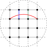
Figure 8. A $4\times 4$ cell with the edges $e_{\lambda},e_{1},e_{2}$ colored in red, blue, green, respectively.

Let $\psi(e_{\lambda}),\psi(e_{1}),\psi(e_{2})$ be the Grassmann monomials defined in (3.28) (we drop the index $\theta$). From the definition (3.35), one can check that the potential satisfies $V(\psi)=F(\psi)$ and that it is given by

$$V(\psi)=\varepsilon_{\emptyset}^{\{e_{\lambda}\}}\psi(e_{\lambda})+\varepsilon^{\{e_{\lambda}\}}_{\{e_{1}\}}\psi(e_{\lambda})\psi(e_{1})+\varepsilon^{\{e_{\lambda}\}}_{\{e_{2}\}}\psi(e_{\lambda})\psi(e_{2})+\varepsilon^{\{e_{\lambda}\}}_{\{e_{1},e_{2}\}}\psi(e_{\lambda})\psi(e_{1})\psi(e_{2}).$$ (A.1)

The computation of the signs $\varepsilon_{S}^{J}$ can be easily done starting from (3.42) and with the help of Fig. 9; details are left to the reader. The final result is that

$$\varepsilon_{\emptyset}^{\{e_{\lambda}\}}=\varepsilon^{\{e_{\lambda}\}}_{\{e_{1},e_{2}\}}=1,\varepsilon^{\{e_{\lambda}\}}_{\{e_{1}\}}=\varepsilon^{\{e_{\lambda}\}}_{\{e_{2}\}}=-1.$$ (A.2)

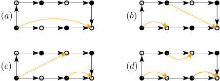
Figure 9. The set of edges $E_{J,S}$ with $J=\{e_{\lambda}\},S=\emptyset$ (drawing (a)), $J={\{e_{\lambda}\},S=\{e_{1}\}}$ (drawing (b)), $J={\{e_{\lambda}\},S=\{e_{2}\}}$ (drawing (c)), $J={\{e_{\lambda}\},S=\{e_{1},e_{2}\}}$ (drawing (d)), colored in orange. Here the orientation of black edges coincides with that on $G^{0}_{L}$ (see Fig. 3), while that of orange edges is the one described in Lemma 2 and in the caption of Figure 6.

References

- [1] M. Aizenman, M. Harel, R. Peled, and J. Shapiro, Depinning in the integer-valued Gaussian Field and the BKT phase of the 2D Villain model, arXiv:2110.09498.
- [2] F. Alet et al, Interacting Classical Dimers on the Square Lattice, Phys. Rev. Lett. 94 (2005), 235702.
- [3] V. Beffara, S. Chhita, K. Johansson, Airy point process at the liquid-gas boundary, Annals of Probability 46 (2018), 2973–3013.
- [4] R. Bauerschmidt, J. Park, P.-F. Rodriguez, The Discrete Gaussian model, I. Renormalisation group flow at high temperature, arXiv:2202.02286
- [5] R. Bauerschmidt, J. Park, P.-F. Rodriguez, The Discrete Gaussian model, II. Infinite-volume scaling limit at high temperature, arXiv:2202.02287
- [6] G. Benfatto, P. Falco, V. Mastropietro: Massless Sine-Gordon and massive Thirring models: proof of Coleman’s equivalence Commun. Math. Phys. 285 (2009) 713–762.
- [7] G. Benfatto, P. Falco, V. Mastropietro: Extended scaling relations for planar lattice models, Commun. Math. Phys. 292 (2009), 569–605.
- [8] G. Benfatto, P. Falco, V. Mastropietro: Universality of One-Dimensional Fermi Systems, I. Response Functions and Critical Exponents, Commun. Math. Phys. 330 (2014), pp.153–215; and II. The Luttinger Liquid Structure, ibid., pp. 217–282.
- [9] G. Benfatto, V. Mastropietro: On the density-density critical indices in interacting Fermi systems, Commun. Math. Phys. 231 (2002), 97–134.
- [10] G. Benfatto, V. Mastropietro: Ward identities and vanishing of the Beta function for interacting Fermi systems, J. Stat. Phys. 115 (2004), 143–184.
- [11] G. Benfatto, V. Mastropietro: Ward identities and chiral anomaly in the Luttinger liquid, Commun. Math. Phys. 258 (2005), 609–655.
- [12] G. Benfatto, V. Mastropietro: Universality relations in non-solvable quantum spin chains, J. Stat. Phys. 138 (2010), 1084–1108.
- [13] G. Benfatto, V. Mastropietro: Drude weight in non solvable quantum spin chains, J. Stat. Phys. 143 (2011), 251–260.
- [14] N. Chandgotia, R. Peled, S. Sheffield, and M. Tassy, Delocalization of uniform graph homomorphisms from to , Commun. Math. Phys. 387 (2021), no. 2, 621–647.
- [15] R. L. Dobrushin, The Gibbs state that describes the coexistence of phases for a three-dimensional Ising model, Teor. Verojatnost. i Primenen., 17 (1972), 619–639.
- [16] H. Duminil-Copin, M. Harel, B. Laslier, A. Raoufi, and G. Ray, Logarithmic variance for the height function of square-ice, Comm. Math. Phys. 396, 867-902 (2022).
- [17] H. Duminil-Copin, A. Karrila, I. Manolescu, and M. Oulamara, Delocalization of the height function of the six-vertex model, arXiv:2012.13750
- [18] P. Falco, Kosterlitz-Thouless transition line for the two-dimensional Coulomb gas, Commun. Math. Phys. 312(2):559-609, 2012
- [19] P. Falco, Critical exponents of the two dimensional Coulomb gas at the Berezinskii-Kosterlitz-Thouless transition, arXiv:1311.2237
- [20] J. Fröhlich and T. Spencer, The Kosterlitz-Thouless transition in two-dimensional abelian spin systems and the Coulomb gas, Comm. Math. Phys. 81 (1981), no. 4, 527–602.
- [21] A. Galluccio, M. Loebl, On the Theory of Pfaffian Orientations. I. Perfect Matchings and Permanents, Elect. J. Combinatorics 6 (1999), #R6
- [22] G. Gentile, V. Mastropietro, Renormalization group for one-dimensional fermions. A review on mathematical results, Phys. Rep. 352, 273-438 (2001).
- [23] T. Giamarchi: Quantum Physics in One Dimension, Oxford University Press, Oxford (2004).
- [24] A. Giuliani, R.L. Greenblatt, V. Mastropietro, The scaling limit of the energy correlations in non integrable Ising models, Jour. Math. Phys. 53, 095214 (2012).
- [25] A. Giuliani, V. Mastropietro, F. L. Toninelli, Height fluctuations in interacting dimers, Ann. Inst. H. Poincaré Probab. Statist. 53(1): 98-168 (2017).
- [26] A. Giuliani, V. Mastropietro, F. L. Toninelli, Haldane relations for interacting dimers, J. Stat. Mech. (2017), 10.1088/1742-5468/aa5d1f.
- [27] A. Giuliani, F. L. Toninelli, Non-integrable dimer models: universality and scaling relations, J. Math. Phys. 60, 103301 (2019).
- [28] A. Giuliani, V. Mastropietro, F. L. Toninelli, Non integrable Dimers: Universal Fluctuations of Tilted Height Profiles, Commun. Math. Phys. 377 (2020), 1883-1959.
- [29] V. Gorin, Lectures on random lozenge tilings, Vol. 193, Cambridge University Press, 2021.
- [30] H. E. Haber, Notes on antisymmetric matrices and the pfaffian, unpublished, available at http://scipp.ucsc.edu/ haber/webpage/pfaffian2.pdf
- [31] O. J. Heilmann, E. Praestgaard, Crystalline ordering in lattice models of hard rods with nearest neighbor attraction, Chem. Phys. 24 (1977), 119–123.
- [32] K. Johansson, The arctic circle boundary and the Airy process, Annals of Probability 33 (2005), 1–30.
- [33] P. W. Kasteleyn, The statistics of dimers on a lattice: I. The number of dimer arrangements on a quadratic lattice, Physica 27, 1209-1225 (1961).
- [34] P. W. Kasteleyn, Dimer statistics and phase transitions, J. Math. Phys. 4 (1963), no. 2, 287-293.
- [35] P. W. Kasteleyn, Graph theory and crystal physics, Graph theory and theoretical physics (1967), 43-110
- [36] R. Kenyon, Local statistics of lattice dimers, Ann. Inst. H. Poincaré, Prob Stat. 33 (1997), 591-618.
- [37] R. Kenyon, Lectures on dimers, Park City Math Institute Lectures, available at arXiv:0910.3129.
- [38] R. Kenyon, A. Okounkov, S. Sheffield, Dimers and Amoebae, Annals Math. 163, 1019-1056 (2006).
- [39] P. Lammers, Height function delocalisation on cubic planar graphs, Probab. Theory Related Fields 182 (1-2):531–550, 2022.
- [40] P. Lammers and S. Ott, Delocalisation and absolute-value-FKG in the solid-on-solid model, Probab. Theory Rel. Fields, to appear, arXiv:2101.05139
- [41] E. H. Lieb, F. Y. Wu: Absence of Mott transition in the 1D Hubbard model, Phys. Rev. Lett. 20 (1968), 1445–1449.
- [42] M. Lis, On Delocalization in the Six-Vertex Model, Commun. Math. Phys. 383 (2021), 1181–1205.
- [43] N. V. Temperley, M. E. Fisher, Dimer problem in statistical mechanics-an exact result, Philos. Mag. 6, 1061-1063 (1961).
- [44] G. Tesler, Matchings in graphs on non-orientable surfaces, Journal of Combinatorial Theory, Series B 78 (2000), no. 2, 198-231.
- [45] A. M. Tsvelik: Quantum Field Theory of Condensed Matter Physics, Cambridge University Press, Cambridge (2007).
- [46] W. Wu, A central limit theorem for square ice, arXiv:2206.12058