A Two-stage Multiband WiFi Sensing Scheme via Stochastic Particle-Based Variational Bayesian Inference

Abstract

Multiband fusion enhances WiFi sensing by jointly utilizing signals from multiple non-contiguous frequency bands. However, in the multi-band WiFi sensing signal model, there are many local optimums in the associated likelihood function due to the existence of high frequency component and phase distortion factors, posing challenges for high-accuracy parameter estimation. To address this, we propose a two-stage scheme equipped with different signal models derived from the original model, where the first-stage coarse estimation is performed using a weighted root MUSIC algorithm to narrow down the search range for the subsequent stage, and the second-stage refined estimation utilizes a Bayesian approach to avoid convergence to bad suboptimal solutions. Specifically, we apply the block stochastic successive convex approximation (SSCA) approach to derive a novel stochastic particle-based variational Bayesian inference (SPVBI) algorithm in the refined stage. Unlike conventional particle-based VBI (PVBI) that optimizes only particle probability and incurs exponential per-iteration complexity with particle count, our more flexible SPVBI algorithm optimizes both the position and probability of each particle. Additionally, it utilizes block SSCA to significantly improve sampling efficiency by averaging over iterations, making it suitable for high-dimensional problems. Extensive simulations demonstrate the superiority of our proposed algorithm over various baseline methods.

I Introduction

Future Wi-Fi networks (e.g., Wi-Fi 7) are expected to achieve integrated sensing and communication (ISAC) functionality [1], where Wi-Fi signals will be exploited to also provide high-accuracy sensing services, such as indoor localization and tracking, activity recognition, in-home digital health, etc [2]. The sensing performance generally depends on the bandwidth of the Wi-Fi signal. However, increasing the bandwidth is not a scalable solution due to limited spectrum resources. Besides, large bandwidth will bring great pressure to signal acquisition, data transmission and processing, which leads to a high hardware costs. Although there have been many improvements in the super-resolution method of single-band signal processing, it is still limited by the fixed signal bandwidth. Such a situation has prompted the recent research interest in multiband WiFi sensing, a technology that provides the potential to improves the resolution and range accuracy by making use of the channel state information (CSI) measurements across multiple non-contiguous frequency bands.

Compared to single-band WiFi sensing, multiband sensing can reap extra multiband gains, which consist of two parts: (i) Bandwidth-related apertures gains resulted from multiband observations; (ii) Band gap apertures gains brought by the difference of carrier frequency between subbands [3]. The different apertures and spectrum distribution are shown in Fig. 1, and details will be explained in the following sections.

Despite the existence of the multiband gains, the multiband WiFi sensing technology comes with unique challenges. One challenge is that the high frequency carrier leads to a violent oscillation phenomenon of the likelihood function, resulting in numerous bad local optimums around the truth value of the delay. As a result, finding the global optimum of the target parameter becomes intractable. The other challenge is the phase misalignment of the received multiband signals caused by hardware imperfections [4, 5]. Per-band channel impulse response (CIR) measurements are superimposed with a random initial phase and a time synchronization error, which are independent from one band to the other. If the phase calibration process is not executed or the calibration precision is insufficient, the sensing performance may be poor. Therefore, it is extremely difficult to fully exploit this apertures gains especially in the presence of phase distortion factors.

The existing multi-band sensing methods can be divided into three categories: subspace based method, compressed sensing based method and probabilistic inference based method. These related works are summarized in Table. I. Unfortunately, these methods have at least one of the limitations as listed below: (i) Underlying band gap apertures gain from multiband is not fully exploited; (ii) Failure to achieve low cost calibration of phase distortion factors. Consequently, we propose a two-stage multiband Wi-Fi sensing scheme via stochastic particle-based variational Bayesian inference (SPVBI) to overcome these limitations. The main contributions are summarized as follows.

TABLE I: A BRIEF SUMMARY OF THE EXISTING MULTIBAND SENSING METHODS.

Category	One sentence summary	Publication	Pros	Cons
Subspace based	Leverage the special structure in multiband signal subspace to achieve estimation	[3, 6, 7, 8, 9]	Low computational complexity	Sensitive to model error and noise interference
Compressed sensing based	Exploit sparsity of multipath channel in delay domain to achieve estimation	[5, 10, 11, 12]	No need to determine the number of scattering paths	(i) Require dense grids; (ii) High computational complexity
Probabilistic Inference based	(i) Maximum likelihood estimation; (ii) Bayesian inference	[13, 14]	(i) Exploit prior information; (ii) High estimation accuracy	(i) Easy to fall into local optimum; (ii)Complicated algorithm design

• Two-stage parameter estimation framework: The conventional two-stage framework adopted the same signal model but different estimation algorithms. However, in our proposed two-stage estimation here, different signal models derived from the original model are adopted, and associated two-stage estimation algorithms are designed according to the statistical characteristics of different models. Specifically, in the coarse estimation stage, a simple but stable MUSIC-based coarse estimation is used to narrow down the search range, so that numerous ’bad’ local optimums can be excluded from the global search space in the refined estimation stage. In the refined estimation stage, we adopt a modified particle-based VBI method, which can make full use of the intrinsic band gap aperture gain in the multiband refined signal model to improve the estimation accuracy.

• Stochastic particle-based variational Bayesian inference: The proposed SPVBI algorithm uses three innovative ideas to achieve accurate posteriori estimation of target parameters with reduced complexity and fast convergence speed. First, we adopt the particle-based approximation to transform the multiple integral operation in VBI into multiple weighted summation. Second, particle positions are updated in each iteration to minimize the VBI objective function. Such improved degree of freedom can further enhance the performance and accelerate the convergence speed. Third, to avoid the exponential complexity with the number of particles, we extend the SSCA approach in [15] to block SSCA and apply it to improve the sampling efficiency of the expectation operator in VBI iteration using the average-over-iteration technique.

• Rigorous convergence analysis of SPVBI: As an extension of existing SSCA, SPVBI allows block-wise update by constructing a series of parallel sub-surrogate functions, which poses new challenges for theoretical analysis due to asynchronous update. Furthermore, with the update of particles in each iteration, the distribution of random states is no longer constant, but changes dynamically, which is challenging for the theoretical proof. Despite these challenges, we prove that SPVBI is guaranteed to converge to a stationary point of the VBI problem, even though the number of samples used to calculate the expectation in each iteration is fixed as a constant that does not increase with the number of adopted particles.

The rest of the paper is organized as follows. In Section II, we introduce the system model and the original estimation problem in the multi-band WiFi sensing scenario, and propose a novel two-stage signal model. In Section III, we present a two-stage estimation framework. In Section IV, we introduce the SPVBI algorithm for the second stage, along with an analysis of its convergence. In Section V, we present numerical simulations and a performance analysis. Finally, conclusions are presented in Section VI.

Notations: $\delta(\cdot)$ denotes the Dirac’s delta function, $\mathop{{\rm var}}(\cdot)$ denotes the variance operator, and $\left\|\cdot\right\|$ denotes the Euclidean norm. For a matrix $\mathbf{A}$, $\mathbf{A}^{T}$ , $\mathbf{A}^{H}$, $\mathbf{A}^{-1}$, represent a transpose, complex conjugate transpose and inverse, respectively. $\mathbb{E}_{z}[\cdot]$ denotes the expectation operator with respect to the random vector $z$. $\boldsymbol{D}_{KL}\left[q\left\|p\right.\right]$ denotes the Kullback-Leibler (KL) divergence of the probability distributions $q$ and $p$. $\mathcal{N}(\mu,\Sigma)$ and $\mathcal{CN}(\mu,\Sigma)$ denotes Gaussian and complex Gaussian distribution with mean $\mu$ and covariance matrix $\Sigma$.

II System Model and Problem Formulation

II-A System Model

In the scene of multi-band WiFi sensing, we consider a single-input single-output (SISO) system that uses OFDM training signals over $M$ frequency subbands to estimate range between the mobile node and Wi-Fi device. The indoor radio propagation channel $h\left(t\right)$ between transceivers is modeled as the sum of $K$ multipath components given by

$$h_{m}\left(t\right)=\sum\limits_{k=1}^{K}\alpha_{k}e^{j\beta_{k}}\delta\left(t-\tau_{k}\right),$$ (1)

where $m=1,2,\ldots M$ is the frequency band index, $\alpha_{k}e^{j\beta_{k}}$ is the complex gain carrying the amplitude and phase information of a scattering path, and $\tau_{k}$ is the time delay of the $k$-th path. Without loss of generality, we assume $\tau_{1}<\tau_{2}<\ldots<\tau_{K}$. Therefore, $\tau_{1}$ represents the delay of line-of-sight (LoS) path which is considered to be estimated for ranging.

Taking the Fourier transform of (1), the discrete frequency-domain channel response can be expressed as

$$h_{m}\left(n\right)=\sum\limits_{k=1}^{K}\alpha_{k}e^{j\beta_{k}}e^{-j2\pi\left(f_{c,m}+nf_{s,m}\right)\tau_{k}},$$ (2)

where $n=0,1,\ldots N_{m}-1$ denotes subcarrier index, $N_{m}$ denotes the number of subcarriers in each band. $f_{c,m}$ and $f_{s,m}$ are the initial frequency and subcarrier spacing of $m$-th frequency band, respectively.

Unfortunately, The pilot signals in a WiFi device are subject to the phase distortion due to hardware imperfections as well as additive noise. Specifically, due to the packet detection delay (PDD) and receiver sampling frequency offset (SFO) [4, 16, 17], there is a timing synchronization error $\delta_{m}$ in the CSI measurements of $m$-th frequency band. In addition, due to the hardware difference, the CSI measurements are superimposed with a random initial phase $\phi_{m}$ [18]. These two imperfect factors are obstacles for multi-band signal fusion and need to be calibrated.

After removing the known training signals, the discrete frequency-domain received signal model during the period of a single OFDM symbol can be formulated as [3, 10]

$$r_{m}^{\left(n\right)}=\sum\limits_{k=1}^{K}\alpha_{k}e^{j\beta_{k}}e^{-j2\pi\left(f_{c,m}+nf_{s,m}\right)\left(\tau_{k}+\delta_{m}\right)}e^{j\phi_{m}}+w_{m}^{\left(n\right)},$$ (3)

$w_{m}^{\left(n\right)}$ denotes an additive white Gaussian noise (AWGN) following the distribution $\mathcal{CN}\left(0,\eta_{w}^{2}\right)$.

Figure 1: An illustration of multi-band WiFi system and spectrum distribution.

II-B Problem Formulation

In multiband sensing problem, the variables to be estimated are denoted as $\mathbf{\boldsymbol{\Lambda}_{ori}}{\rm=}\left[\alpha_{1},\ldots,\alpha_{K},\tau_{1},\ldots,\tau_{K},\beta_{1},\ldots,\beta_{K},\right.$ $\left.\phi_{1},\ldots,\phi_{M},\delta_{1},\ldots,\delta_{M}\right]^{T}$, and frequency domain measurements of the received signal is vectorized as $\boldsymbol{r}=\left[r_{1}^{\left(0\right)},r_{1}^{\left(1\right)},\ldots,r_{1}^{\left(N_{1}-1\right)},\right.$ $\left.\ldots,r_{M}^{\left(0\right)},r_{M}^{\left(1\right)},\ldots,r_{M}^{\left(N_{M}-1\right)}\right]^{T}$.

In the case of AWGN, the logarithmic likelihood function of the original signal model (3) can be written as follow

$$\begin{split}&\ln p\left(\boldsymbol{r}|\mathbf{\boldsymbol{\Lambda}_{ori}}\right)=\ln\prod\limits_{m=1}^{M}\prod\limits_{n=0}^{N_{m}-1}p(r_{m}^{\left(n\right)}|\mathbf{\boldsymbol{\Lambda}_{ori}})\\ &=MN_{m}\ln\frac{1}{\sqrt{2\pi}\eta_{w}}-\sum_{m=1}^{M}\sum_{n=0}^{N_{m}-1}\frac{1}{2\eta_{w}^{2}}\left|r_{m}^{\left(n\right)}-s_{m}^{\left(n\right)}\left(\mathbf{\boldsymbol{\Lambda}_{ori}}\right)\right|^{2},\end{split}$$ (4)

$$\begin{split}s_{m}^{\left(n\right)}\left(\mathbf{\boldsymbol{\Lambda}_{ori}}\right)&=\sum\limits_{k=1}^{K}\alpha_{k}e^{j\beta_{k}}e^{-j2\pi(f_{c,m}+nf_{s,m})\tau_{k}}\\ &e^{j\phi_{m}}e^{-j2\pi\left(f_{c,m}+nf_{s,m}\right)\delta_{m}},\end{split}$$ (5)

where $s_{m}^{\left(n\right)}\left(\mathbf{\boldsymbol{\Lambda}_{ori}}\right)$ is the received signal reconstructed from the parameter $\mathbf{\boldsymbol{\Lambda}_{ori}}$.

Based on the above likelihood function and some given prior, we wish to obtain the maximum a posteriori (MAP) estimate of the target parameters by solving such a maximization problem:

$$\begin{split}\mathcal{P}_{\mathbf{\boldsymbol{\mathrm{ori}}}}:\mathbf{\left(\boldsymbol{\Lambda}_{ori}^{*}\right)_{MAP}=}\mathrm{arg}\mathop{\mathrm{max}}\limits_{\mathbf{\mathbf{\boldsymbol{\Lambda}_{ori}}}}\quad&\ln\left[p\left(\boldsymbol{r}|\mathbf{\boldsymbol{\Lambda}_{ori}}\right)p\left(\mathbf{\boldsymbol{\Lambda}_{ori}}\right)\right]\end{split},$$ (6)

where the joint posteriori probability can be easily deduced from the Bayes equation $p\left(\boldsymbol{\Lambda}|\boldsymbol{r}\right)\propto p\left(\boldsymbol{r}|\boldsymbol{\Lambda}\right)p\left(\boldsymbol{\Lambda}\right)$.

However, the global parameter estimation problem will be intractable if we directly use the signal model (3). On the one hand, the multi-dimensional parameters make the search space of the estimation problem very huge. On the other hand, there are many local optimums in the likelihood function (4). Motivated by the these challenges, we next set up the novel two-stage signal model and customize the associated two-stage global estimation scheme.

II-C Two-stage Signal Model

Prior to presenting the details of two-stage signal model, it is important to note some features about the likelihood function in this problem.

According to the above expression of the likelihood function (4), we can plot the spectrum of the likelihood function with respect to time delay by fixing other variables. As shown by the solid pink line in Fig. 2, the likelihood function fluctuates periodically, with a sharp main lobe appearing at the location of the true value point, accompanied by many oscillating side lobes.

As can be seen in (4), the period of this oscillation phenomenon is affected by the frequency term $(f_{c,m}+nf_{s,m})$, which is multiplied by the delay term $\tau_{k}$. Once the WiFi carrier frequency reaches several to tens of GHz, this will inevitably lead to violent oscillations of the likelihood function with a period of nanoseconds. As a result, finding the global optimum becomes intractable. Moreover, when the signal-to-noise ratio (SNR) is not high and there are imperfect factors, the estimate may deviate to the locally optimal side-lobe, resulting in a degradation of the estimation performance.

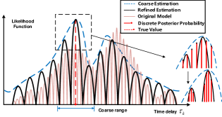
Figure 2: An illustration of oscillation phenomena and particle approximation.

Therefore, we divide the target parameter estimation into two stages equipped with different signal models derived from the original model in (3). These two signal models have the structures of bandwidth aperture and band gap aperture [19] respectively, which are presented in Fig. 1 and will be explained below.

(1) Coarse signal model with the bandwidth aperture $(nf_{s,m})$ structure:

$$\begin{split}r_{m}^{\left(n\right)}&=\sum\limits_{k=1}^{K}\alpha_{k,m}^{{}^{\prime}}e^{-j2\pi(nf_{s,m})\left(\tau_{k}+\delta_{m}\right)}+w_{m}^{\left(n\right)},\end{split}$$ (7)

where $\alpha_{k,m}^{{}^{\prime}}=\alpha_{k}e^{j\beta_{k}}\cdot e^{j\phi_{m}}e^{-j2\pi f_{c,m}\left(\tau_{k}+\delta_{m}\right)}$.

In the coarse estimation stage, the carrier phase $e^{-j2\pi f_{c,m}\left(\tau_{k}+\delta_{m}\right)}$ and the random phase $e^{j\phi_{m}}$ of each band are absorbed into the complex scalar $\alpha_{k}e^{j\beta_{k}}$, while the bandwidth term $nf_{s,m}$ is retained, so that all sub-bands share a bandwidth-dependent delay domain, which we call the bandwidth aperture.

As shown by the dotted blue line in Fig. 2, the bandwidth aperture smoothes the likelihood function, so that the true value can most likely be found in the peak region of the main lobe, thus obtaining a relatively rough but stable estimate.

(2) Refined signal model with the band gap aperture $(f_{c,m}^{{}^{\prime}}+nf_{s,m})$ structure:

$$\begin{split}r_{m}^{\left(n\right)}&=\sum\limits_{k=1}^{K}\alpha_{k}^{{}^{\prime}}e^{j\beta_{k}^{{}^{\prime}}}e^{-j2\pi(f_{c,m}^{{}^{\prime}}+nf_{s,m})\tau_{k}}\\ &e^{j\phi_{m}^{{}^{\prime}}}e^{-j2\pi nf_{s,m}\delta_{m}}+w_{m}^{\left(n\right)},\end{split}$$ (8)

where, $\alpha_{k}^{{}^{\prime}}e^{j\beta_{k}^{{}^{\prime}}}=\alpha_{k}e^{j\beta_{k}}\cdot e^{j\tilde{\phi}_{1}}e^{-j2\pi f_{c,1}\tau_{k}}$, $\phi_{m}^{{}^{\prime}}=\tilde{\phi}_{m}-\tilde{\phi}_{1}$, $f_{c,m}^{{}^{\prime}}=f_{c,m}-f_{c,1}$, $\phi_{1}^{{}^{\prime}}=0$, $f_{c,1}^{{}^{\prime}}=0$.

In the stage of refined estimation, we first absorb the term $e^{-j2\pi f_{c,m}\delta_{m}}$ into the initial phase $e^{j\phi_{m}}$, namely $e^{j\tilde{\phi}_{m}}{\rm=}e^{j\left(\phi_{m}-2\pi f_{c,m}\delta_{m}\right)}$, which also aims to reduce the oscillation degree of the likelihood function in the estimation of $\delta_{m}$. Then, if we take the first frequency band as a reference, the rewritten initial phase $e^{j\tilde{\phi}_{1}}$ and the carrier phase $e^{-j2\pi f_{c,1}\tau_{k}}$ can be absorbed into the complex scalar $\alpha_{k}e^{j\beta_{k}}$ of each path, and the residual band gap term $e^{-j2\pi(f_{c,m}-f_{c,1}+nf_{s,m})\tau_{k}}$ is retained in each sub-band signal, which is therefore called the band gap aperture structure.

Fig. 2 illustrates that the oscillation of likelihood function associated with the refined signal model will not be too violent, at the same time, the main lobe becomes sharper than that of the coarse estimation model. In this case, we can exploit the multi-band gain (i.e, the more sensitive phase rotation caused by the gap between the carrier frequencies) to improve the performance.

III Two-stage Estimation Framework

Based on the two-stage signal model, the two-stage estimation framework is depicted as follow.

III-A Coarse Estimation

In the coarse estimation stage, we first need to determine the number of scattering paths $K$. To the best of our knowledge, Akaike Information Criterion (AIC) [20] or the Minimum Description Length (MDL) [21] are both efficient methods that generally work well, which will not be described here for conciseness. Then, we use the weighted root-MUSIC (WR-MUSIC) [7, 22] algorithm to roughly estimate the delay $\tau_{k}$. The coarse estimate signal model (7) can be written in the following form:

$$\boldsymbol{\mathbf{Y}}_{m}=\boldsymbol{\mathbf{X}}_{m}\boldsymbol{\mathbf{A}}_{m}+\boldsymbol{w}_{m},$$ (9)

where

$$\begin{cases}\boldsymbol{\mathbf{Y}}_{m}{\rm=}\left[r_{m}^{\left(0\right)},r_{m}^{\left(1\right)},\ldots,r_{m}^{\left(N_{m}-1\right)}\right]^{T},\\ \boldsymbol{\mathbf{X}}_{m}(\boldsymbol{\mathbf{\tau}}){\rm=}\left[\boldsymbol{\mathbf{x}}(\tau_{1}+\delta_{m}),\boldsymbol{\mathbf{x}}(\tau_{2}+\delta_{m}),\cdots,\mathbf{\boldsymbol{x}}(\tau_{K}+\delta_{m})\right],\\ \boldsymbol{\mathbf{x}}(\mathring{\tau}){\rm=}[1,e^{-j2\pi f_{s,m}\mathring{\tau}},\cdots,e^{-j2\pi(N_{m}-1)f_{s,m}\mathring{\tau}}]^{T},\\ \mathbf{\boldsymbol{A}}_{m}{\rm=}[\alpha_{1,m}^{{}^{\prime}},\alpha_{2,m}^{{}^{\prime}},\cdots,\alpha_{K,m}^{{}^{\prime}}]^{T},\\ \boldsymbol{w}_{m}=[w_{m}^{\left(0\right)},w_{m}^{\left(1\right)},\cdots,w_{m}^{\left(N_{m}-1\right)}]^{T},\end{cases}$$ (10)

and $\boldsymbol{\mathbf{\tau}}=\left[\tau_{1},...,\tau_{K}\right]^{T}$. Since the coarse estimation aims to simply reduce the search range with low complexity and doesn’t require high accuracy, it’s reasonable to use such a simplified form even if it may introduce some model distortion.

Next according to the WR-MUSIC algorithm, we can construct a Hankel matrix for subspace decomposition of the received signal [23], in the following form:

$$\boldsymbol{H}_{m}=\left[\begin{array}[]{cccc}r_{m}^{\left(0\right)}&r_{m}^{\left(1\right)}&\cdots&r_{m}^{\left(L-1\right)}\\ r_{m}^{\left(1\right)}&r_{m}^{\left(2\right)}&\cdots&r_{m}^{\left(L\right)}\\ \vdots&\vdots&\ddots&\vdots\\ r_{m}^{\left(N_{m}-L\right)}&r_{m}^{\left(N_{m}-L+1\right)}&\cdots&r_{m}^{\left(N_{m}-1\right)}\end{array}\right],$$ (11)

where $L$ is the length of correlation window, empirically taken as $\nicefrac{{N_{m}}}{{3}}$ [24].

After that, we apply the eigenvalue decomposition to the Hankel matrix of the signal, $\boldsymbol{H}_{m}=\boldsymbol{U}_{m}\boldsymbol{D}_{m}\boldsymbol{V}_{m}^{H}$. The eigenspace composed of the eigenvectors corresponding to the largest $K$ (i.e. the number of scattering paths) eigenvalues is called the signal subspace and is denoted as $\boldsymbol{\mathbf{S}}_{signal}$. The eigenspace composed of the eigenvectors corresponding to the remaining $(N_{m}-K)$ eigenvalues is called the noise subspace and denoted as $\boldsymbol{\mathbf{S}}_{noise}$.

Essentially, compared with the conventional MUSIC algorithm, the root MUSIC algorithm [22] is to apply the polynomial root-finding method to replace the spectral search of zeros. Define the polynomial: $f_{l}\left(z\right)=\mathbf{u}_{l}^{H}\mathbf{p}\left(z\right),l=K+1,\ldots N_{m}$, where $\mathbf{u}_{l}^{H}$ is the $l$-th eigenvector of noise subspace $\boldsymbol{\mathbf{S}}_{noise}$, $\mathbf{p}\left(z\right)=[1,z,\cdots,z^{N_{m}-1}]^{T}$, and $z=e^{-j2\pi f_{s,m}\tau}$. In order to utilize all noise eigenvectors, we wish to find the zeros of the following polynomials:

$$f\left(z\right)=\mathbf{p}^{H}\left(z\right)\mathbf{S}_{noise}\mathbf{S}_{noise}^{H}\mathbf{p}\left(z\right).$$ (12)

We rewrite (12) to get the polynomial in terms of $z$ as:

$$f\left(z\right)=z^{N_{m}-1}\mathbf{p}^{T}\left(z^{-1}\right)\mathbf{S}_{noise}\mathbf{S}_{noise}^{H}\mathbf{p}\left(z\right).$$ (13)

Find the roots of the above polynomial, wherein the $K$ roots in the unit circle whose moduli are closest to $1$ contain the information about delay. Denote those roots as $p_{k,m},k=1,2\ldots K$, then the coarse estimate of the delay can be obtained: $\hat{\tau}_{k,m}=\frac{arg\left(p_{k,m}\right)}{-2\pi f_{s,m}}$. We can further improve the delay estimation accuracy by combining the results of different frequency band according to the Cramér-Rao bound (CRB) analysis [7]:

$$\hat{\tau}_{k}=\frac{\sum_{m=1}^{M}SNR_{m}\cdot B_{m}\cdot\left(f_{c,m}^{2}+B_{m}^{2}/12\right)\cdot\hat{\tau}_{k,m}}{\sum_{m=1}^{M}SNR_{m}\cdot B_{m}\cdot\left(f_{c,m}^{2}+B_{m}^{2}/12\right)}.$$ (14)

Also, the estimate of $\alpha_{k,m}^{{}^{\prime}}$ can be obtained by the least square (LS) method:

$$\boldsymbol{\mathbf{\hat{A}}}_{m}=\left(\boldsymbol{\mathbf{X}}_{m}^{H}(\hat{\boldsymbol{\tau}})\boldsymbol{\mathbf{X}}_{m}(\hat{\boldsymbol{\tau}})\right)^{-1}\boldsymbol{\mathbf{X}}_{m}^{H}(\hat{\boldsymbol{\tau}})\boldsymbol{\mathbf{Y}}_{m}.$$ (15)

where $\hat{\boldsymbol{\tau}}=\left[\hat{\tau}_{1},...,\hat{\tau}_{K}\right]$, $\boldsymbol{\mathbf{\hat{A}}}_{m}=[\hat{\alpha}_{1,m}^{{}^{\prime}},\hat{\alpha}_{2,m}^{{}^{\prime}},\cdots,\hat{\alpha}_{K,m}^{{}^{\prime}}]^{T}$. Then, the signal can be written as an all-pole model [24]:

$$r_{m}^{\left(n\right)}=\sum\limits_{k=1}^{K}\hat{\alpha}_{k,m}^{{}^{\prime}}\left(e^{-j2\pi f_{s,m}\hat{\tau}_{k,m}}\right)^{n}=\sum\limits_{k=1}^{K}\hat{\alpha}_{k,m}^{{}^{\prime}}p_{k,m}^{n}.$$ (16)

By comparing the terms in equations (7) and (16), the difference between the random initial phases of the two bands can be estimated as follows:

$$\begin{split}\hat{\phi}_{m}^{{}^{\prime}}=&\hat{\phi}_{m}-\hat{\phi}_{1}=\frac{1}{K}\sum\limits_{k=1}^{K}\left[arg\left(\hat{\alpha}_{k,m}^{{}^{\prime}}\right)-arg\left(\hat{\alpha}_{1,m}^{{}^{\prime}}\right)\right.\\ &\left.-2\pi f_{c,1}\left(\hat{\tau}_{k,1}\right)+2\pi f_{c,m}\left(\hat{\tau}_{k\text{,m}}\right)\right].\end{split}$$ (17)

Then we can also get

$$\hat{\delta}_{m}=\frac{1}{K}\sum\limits_{k=1}^{K}\left[\frac{arg\left(p_{k,m}\right)}{-2\pi f_{s,m}}-\hat{\tau}_{k}\right].$$ (18)

Therefore, in the coarse estimation stage, we can obtain coarse estimate of delay $\hat{\tau}_{k}$, complex gain amplitude $\left\|\widehat{\alpha}_{k}\right\|$ (i.e. $\frac{\sum_{m=1}^{M}SNR_{m}\cdot B_{m}\cdot\left(f_{c,m}^{2}+B_{m}^{2}/12\right)\cdot\left\|\hat{\alpha}_{k,m}^{{}^{\prime}}\right\|}{\sum_{m=1}^{M}SNR_{m}\cdot B_{m}\cdot\left(f_{c,m}^{2}+B_{m}^{2}/12\right)}$), difference between the random initial phases $\hat{\phi}_{m}^{{}^{\prime}}$ and timing synchronization error $\hat{\delta}_{m}$ to serve the refined estimation.

In addition, coarse estimates and reasonable prior assumptions together provide prior information for the subsequent stage. As mentioned earlier, the truth value $\tau_{k}$ will most likely fall in the neighborhood of the coarse estimate $[\hat{\tau}_{k}-\Delta\hat{\tau}_{k}/2,\hat{\tau}_{k}+\Delta\hat{\tau}_{k}/2]$. The interval of refined estimation $\Delta\hat{\tau}_{k}$ can be determined according to the empirical error of the first stage, or several times of the square root of the CRB calculated based on the coarse estimate. Although a relatively accurate estimate of $\left\|\widehat{\alpha}_{k}\right\|$ is obtained in the first stage, its phase is still unknown. It can be assumed that the phase is uniformly distributed from $0$ to $2\pi$. The prior probability distributions for $\phi_{m}^{{}^{\prime}}$ and $\beta_{k}^{{}^{\prime}}$ are similar. Since the timing synchronization error $\delta_{m}$ is often within a small interval, it can be assumed that it follows a prior distribution $\mathcal{N}\left(0,\sigma^{2}\right)$ with a relatively small variance $\sigma^{2}$ [4].

III-B Refined Estimation

Correspondingly, variables to be estimated in the refined stage are adjusted as $\mathbf{\boldsymbol{\Lambda}}{\rm=}\left[\alpha_{1}^{{}^{\prime}},\ldots,\alpha_{K}^{{}^{\prime}},\tau_{1},\ldots,\tau_{K},\right.$ $\left.\beta_{1}^{{}^{\prime}},\ldots,\beta_{K}^{{}^{\prime}},\phi_{2}^{{}^{\prime}},\ldots,\phi_{M}^{{}^{\prime}},\delta_{1},\ldots,\delta_{M}\right]^{T}$ and the total number of variables is denoted as $\left|\boldsymbol{\Lambda}\right|=J$. In the logarithmic likelihood function (4), $s_{m}^{\left(n\right)}$ is also adjusted to

$$\begin{split}s_{m}^{\left(n\right)}\left(\boldsymbol{\Lambda}\right)&=\sum\limits_{k=1}^{K}\alpha_{k}^{{}^{\prime}}e^{j\beta_{k}^{{}^{\prime}}}e^{-j2\pi(f_{{}_{c,m}}^{{}^{\prime}}+nf_{s,m})\tau_{k}}\\ &e^{j\phi_{m}^{{}^{\prime}}}e^{-j2\pi\left(nf_{s,m}\right)\delta_{m}}.\end{split}$$ (19)

In summary, we provide a two-stage estimation scheme as shown in Algorithm 1, which divides the estimation process into coarse estimation stage and refined estimation stage.

Algorithm 1 Two-stage Estimation Scheme

Input: received signals $\boldsymbol{r}$, multi-band frequency settings.

Stage 1: Coarse Estimation

      Construct signal model with the bandwidth

      aperture structure (7);

      Perform WR-MUSIC and LS method;

      Provide coarse estimates and prior intervals for Stage 2.

Stage 2: Refined Estimation

      Construct signal model with the band gap

      aperture structure (8);

      Perform SPVBI algorithm to obtain the approximate

      marginal posteriori probability.

Output: Obtain the MAP/MMSE estimates of each variable based on approximate marginal posteriori probability.

In the coarse estimation stage, WR-MUSIC algorithm and LS method are used to obtain the rough estimates, providing prior information for subsequent estimation and narrowing the search interval. In the next section, we shall propose a SPVBI algorithm to find the approximate marginal posteriori of the target parameters $\boldsymbol{\Lambda}$ for the refined estimation stage.

IV Stochastic Particle-Based Variational Bayesian Inference

IV-A Problem Formulation for SPVBI

In the original MAP estimation problem (6), we need to derive marginal posteriori probability distribution $p\left(\mathbf{\boldsymbol{\Lambda}}_{j}|\boldsymbol{r}\right)$ to perform posteriori inference on the target parameters, where $\mathbf{\mathbf{\boldsymbol{\Lambda}}}_{j}$ represents the $j$-th variable to be estimated in $\mathbf{\boldsymbol{\Lambda}}$. In general, it is intractable to get a closed-form solution for $p\left(\mathbf{\boldsymbol{\Lambda}}_{j}|\boldsymbol{r}\right)$, since it is necessary to integrate all the other variables except $\mathbf{\boldsymbol{\Lambda}}_{j}$ [25] (i.e., multiple expectation operation). To deal with this, many existing works make prior assumptions, such as assuming that the distribution of these variables comes from certain special distribution families [26] or meets the conjugation condition. However, these assumptions are often not accurate enough and can be subjective.

In [27], the authors proposed a particle-based VBI (PVBI) algorithm to approximate the expectation calculation using importance sampling method [28], which is a type of Monte Carlo method. By iteratively updating the weight of particles, the discrete distribution composed of particles $q\left(\mathbf{\mathbf{\boldsymbol{\Lambda}}}_{j}\right)$ can gradually approach the true posteriori probability distribution $p\left(\mathbf{\boldsymbol{\Lambda}}_{j}|\boldsymbol{r}\right)$.

The discrete variational posteriori probability $q\left(\mathbf{\mathbf{\boldsymbol{\Lambda}}}_{j}\right)$ can be written as the weighted sum of $N_{p}$ discrete particles [27]:

$$q\left(\mathbf{\mathbf{\boldsymbol{\Lambda}}}_{j};\mathbf{x}_{j},\mathbf{y}_{j}\right){\rm=}\sum\limits_{p=1}^{N_{p}}y_{j,p}\delta\left(\mathbf{\boldsymbol{\Lambda}}_{j}-x_{j,p}\right),$$ (20)

where $\mathbf{x}_{j}=\left[x_{j,1},x_{j,2},...,x_{j,N_{p}}\right]^{T}$ and $\mathbf{y}_{j}=\left[y_{j,1},y_{j,2},...,y_{j,N_{p}}\right]^{T}$ are the positions and weights of the particles, respectively. Furthermore, according to the mean field assumption [29], the approximate posteriori probability of each variable can be assumed to be independent of each other, $q\left(\boldsymbol{\Lambda};\mathbf{x},\mathbf{y}\right)=\stackrel{{\scriptstyle[}}{{j}}=1]{J}{\prod}q\left(\boldsymbol{\Lambda}_{j};\mathbf{x}_{j},\mathbf{y}_{j}\right)$, where $\mathbf{x}=\left[\mathbf{x}_{1};\mathbf{x}_{2};...;\mathbf{x}_{J}\right]$ and $\mathbf{y}=\left[\mathbf{y}_{1};\mathbf{y}_{2};...;\mathbf{y}_{J}\right]$. Next, the positions and weights $\mathbf{x},\mathbf{y}$ are chosen to minimize the Kullback-Leibler (KL) divergence between the variational probability distribution $q\left(\mathbf{\boldsymbol{\Lambda}};\mathbf{x},\mathbf{y}\right)$ and the real posteriori probability distribution $p\left(\mathbf{\boldsymbol{\Lambda}}|\boldsymbol{r}\right)$ [25], which is defined as

$$\begin{split}\boldsymbol{D}_{KL}\left[q\left\|p\right.\right]&{\rm=}\int q\left(\mathbf{\boldsymbol{\Lambda}};\mathbf{x},\mathbf{y}\right)\ln\frac{q\left(\mathbf{\mathbf{\boldsymbol{\Lambda}}};\mathbf{x},\mathbf{y}\right)}{p\left(\mathbf{\boldsymbol{\Lambda}}|\boldsymbol{r}\right)}d\mathbf{\boldsymbol{\Lambda}}\\ &{\rm=}\int q\left(\mathbf{\boldsymbol{\Lambda}};\mathbf{x},\mathbf{y}\right)\ln\frac{q\left(\mathbf{\mathbf{\boldsymbol{\Lambda}}};\mathbf{x},\mathbf{y}\right)p\left(\boldsymbol{r}\right)}{p\left(\boldsymbol{r}|\mathbf{\boldsymbol{\Lambda}}\right)p\left(\mathbf{\boldsymbol{\Lambda}}\right)}d\mathbf{\mathbf{\boldsymbol{\Lambda}}}.\end{split}$$ (21)

Considering that $p\left(\boldsymbol{r}\right)$ is a constant independent of $q\left(\mathbf{\boldsymbol{\Lambda}};\mathbf{x},\mathbf{y}\right)$, minimizing the KL divergence is equivalent to solving the following optimization problem:

$$\begin{split}\mathcal{P}:\mathop{\min}\limits_{\mathbf{x},\mathbf{y}}\quad&\boldsymbol{L}\left(\mathbf{x},\mathbf{y}\right)\triangleq\int q\left(\boldsymbol{\Lambda};\mathbf{x},\mathbf{y}\right)\ln\frac{q\left(\boldsymbol{\Lambda};\mathbf{x},\mathbf{y}\right)}{p\left(\boldsymbol{r}|\boldsymbol{\Lambda}\right)p\left(\boldsymbol{\Lambda}\right)}d\boldsymbol{\Lambda}\\ \text{s.t.}\quad&\sum\limits_{p=1}^{N_{p}}y_{j,p}=1,\quad\epsilon\leq y_{j,p}\leq 1,\quad\forall j,p,\\ &\hat{\boldsymbol{\Lambda}}_{j}-\Delta\hat{\boldsymbol{\Lambda}}_{j}/2\leq x_{j,p}\leq\hat{\boldsymbol{\Lambda}}_{j}+\Delta\hat{\boldsymbol{\Lambda}}_{j}/2,\quad\forall j,p,\end{split}$$

where $p=1,2,\ldots N_{p}$ and $j=1,2,\ldots J$ are the particle index and variables index, respectively. $\boldsymbol{L}\left(\mathbf{x},\mathbf{y}\right)$ denotes the objective function and $\epsilon>0$ is a small number. The normalized weight $y_{j,p}$ represents the probability that the particle is located at position $x_{j,p}$. $\hat{\boldsymbol{\Lambda}}_{j}$ is the coarse estimation obtained in the first stage and $\Delta\hat{\boldsymbol{\Lambda}}_{j}$ is the range of the estimation error of coarse estimation. The truth value is highly likely to be located in the prior interval $\left[\hat{\boldsymbol{\Lambda}}_{j}-\Delta\hat{\boldsymbol{\Lambda}}_{j}/2,\hat{\boldsymbol{\Lambda}}_{j}+\Delta\hat{\boldsymbol{\Lambda}}_{j}/2\right]$, so the particle position is searched wherein to accelerate the convergence rate. Note that it does not make sense to generate particles with very small probabilities in approximate posteriori since these particles contribute very little to the estimator. Therefore, we restrict the probability of each particle $y_{j,p}$ to be larger than a small number $\epsilon$.

The solution of problem $\mathcal{P}$ refers to the marginal posteriori distribution of each variable, from which we can obtain the best posteriori estimate of the target parameter. In the following sections, we will discuss how to solve this problem.

Remark 1.

In conventional PVBI, the position of particles are not updated. Besides, a large number of particles are required to overcome the instability caused by initial random sampling, and ensure that the estimation locally converges to a ’good’ stationary point. As such, the complexity will rocket as the number of variables and particles increases. Motivated by this observcation, we optimize the particle position as well and further design an SPVBI algorithm to solve the new problem with much lower per-iteration complexity than the conventional PVBI algorithm. Adding the optimization of particle positions $\mathbf{x}$ can improve the effectiveness of characterizing the target distribution by discrete particles, and avoid the estimation result falling into the local optimum due to poor initial sampling. Furthermore, updating particle position can reduce the number of required particles, and thus effectively reduce the computational overhead, which will be discussed in detail in the following sections.

IV-B SPVBI Algorithm Design based on Block SSCA

Although updating particle positions can speed up convergence, multiple integration in the objective function $\boldsymbol{L}\left(\mathbf{x},\mathbf{y}\right)$ of $\mathcal{P}$ is still intractable. To solve this problem, we propose a stochastic particle-based variational Bayesian inference algorithm based on the block SSCA to find stationary points of $\mathcal{P}$ with lower computational complexity.

Specifically, we divided the optimization variables into $2J$ blocks $\mathbf{x}_{1}$, $\mathbf{y}_{1}$, $\mathbf{x}_{2}$, $\mathbf{y}_{2}$, … ,$\mathbf{x}_{J}$, $\mathbf{y}_{J}$. Starting from an initial point $\mathbf{x}^{\left(0\right)},\mathbf{y}^{\left(0\right)}$, the SPVBI algorithm alternatively optimizing each block until convergence. Let $\mathbf{x}_{j}^{\left(t\right)},\mathbf{y}_{j}^{\left(t\right)}$ and $\mathbf{x}_{j}^{\left(t+1\right)},\mathbf{y}_{j}^{\left(t+1\right)}$ denote the blocks $\mathbf{x}_{j},\mathbf{y}_{j}$ before and after the update in the $t$-th iteration, respectively. Then in the $t$-th iteration, the $\left(2j-1\right)$-th block $\mathbf{x}_{j}$ is updated by solving the following subproblem:

$$\begin{split}\mathcal{P}_{x_{j}}:\mathop{\min}\limits_{\mathbf{x}_{j}}\quad&\boldsymbol{L}_{j}^{\left(t\right)}\left(\mathbf{x}_{j},\mathbf{y}_{j}^{\left(t\right)}\right)\\ \text{s.t.}\quad&\hat{\boldsymbol{\Lambda}}_{j}-\Delta\hat{\boldsymbol{\Lambda}}_{j}/2\leq x_{j,p}\leq\hat{\boldsymbol{\Lambda}}_{j}+\Delta\hat{\boldsymbol{\Lambda}}_{j}/2,\forall p\end{split}$$

where $\boldsymbol{L}_{j}^{\left(t\right)}\left(\mathbf{x}_{j},\mathbf{y}_{j}\right)=\boldsymbol{L}\left(\mathbf{x}^{\left(t,j\right)},\mathbf{y}^{\left(t,j\right)}\right)$ with $\mathbf{x}^{\left(t,j\right)}=\left[\mathbf{x}_{1}^{\left(t+1\right)}\right.$ $\left.;...;\mathbf{x}_{j-1}^{\left(t+1\right)};\mathbf{x}_{j};\mathbf{x}_{j+1}^{\left(t\right)};...;\mathbf{x}_{J}^{\left(t\right)}\right]$ and $\mathbf{y}^{\left(t,j\right)}=\left[\mathbf{y}_{1}^{\left(t+1\right)};...;\mathbf{y}_{j-1}^{\left(t+1\right)}\right.$ $\left.;\mathbf{y}_{j};\mathbf{y}_{j+1}^{\left(t\right)};...;\mathbf{y}_{J}^{\left(t\right)}\right]$. In other words, $\boldsymbol{L}_{j}^{\left(t\right)}\left(\mathbf{x}_{j},\mathbf{y}_{j}\right)$ is the objective function $\boldsymbol{L}\left(\mathbf{x},\mathbf{y}\right)$ when fixing all other variables as the latest iterate and only treating $\mathbf{x}_{j},\mathbf{y}_{j}$ as variables. It can be shown that

$$\boldsymbol{L}_{j}^{\left(t\right)}\left(\mathbf{x}_{j},\mathbf{y}_{j}\right)=\sum\limits_{p=1}^{N_{p}}y_{j,p}\ln y_{j,p}-\sum\limits_{p=1}^{N_{p}}y_{j,p}\left[\ln p\left(x_{j,p}\right)+\right.$$

$$\sum\limits_{p_{1}=1}^{N_{p}}\cdots\sum\limits_{p_{j-1}=1}^{N_{p}}\sum\limits_{p_{j+1}=1}^{N_{p}}\cdots\sum\limits_{p_{J}=1}^{N_{p}}\widetilde{y}_{\sim j,p_{\sim j}}\left.\ln p\left(\boldsymbol{r}\left|\widetilde{x}_{\sim j,p_{\sim j}},x_{j,p}\right.\right)\right],$$ (22)

where $\widetilde{y}_{\sim j,p_{\sim j}}=\underset{i\neq j}{\prod}y_{i,p_{i}}$ and $\widetilde{x}_{\sim j,p_{\sim j}}=\left\{x_{i,p_{i}}\right\}_{i\neq j}$, which involves a summation of $N_{p}^{J-1}$ terms. As such, the exponential complexity of directly solving $\mathcal{P}_{x_{j}}$ is unacceptable.

To overcome this challenge, we reformulate $\mathcal{P}_{x_{j}}$ to a stochastic optimization problem as

$$\begin{split}\mathcal{P}_{x_{j}}:\mathop{\min}\limits_{\mathbf{x}_{j}}\quad&\boldsymbol{L}_{j}^{\left(t\right)}\left(\mathbf{x}_{j},\mathbf{y}_{j}^{\left(t\right)}\right)\triangleq{\rm\mathbb{E}}_{\boldsymbol{\Lambda}_{\sim j}}\left[g_{j}^{\left(t\right)}\left(\mathbf{x}_{j},\mathbf{y}_{j}^{\left(t\right)};\boldsymbol{\Lambda}_{\sim j}\right)\right]\\ \text{s.t.}\quad&\hat{\boldsymbol{\Lambda}}_{j}-\Delta\hat{\boldsymbol{\Lambda}}_{j}/2\leq x_{j,p}\leq\hat{\boldsymbol{\Lambda}}_{j}+\Delta\hat{\boldsymbol{\Lambda}}_{j}/2,\forall p,\end{split}$$

where $\boldsymbol{\Lambda}_{\sim j}$ represents all the other variables except $\boldsymbol{\Lambda}_{j}$ and ${\rm\mathbb{E}}_{\boldsymbol{\Lambda}_{\sim j}}\left[\cdot\right]$ represents the expectation operator over the probability distribution of variable $\boldsymbol{\Lambda}_{\sim j}$, and

$$g_{j}^{\left(t\right)}\left(\mathbf{x}_{j},\mathbf{y}_{j};\boldsymbol{\Lambda}_{\sim j}\right){\rm=}\sum\limits_{p=1}^{N_{p}}y_{j,p}\ln y_{j,p}-\sum\limits_{p=1}^{N_{p}}y_{j,p}$$

$$\times\left[\ln p\left(x_{j,p}\right)+\ln p\left(\boldsymbol{r}\left|\boldsymbol{\Lambda}_{{\rm\sim}j},x_{j,p}\right.\right)\right].$$ (23)

Then following the idea of SSCA, we replace the objective function $\boldsymbol{L}_{j}^{\left(t\right)}\left(\mathbf{x}_{j},\mathbf{y}_{j}^{\left(t\right)}\right)$ in $\mathcal{P}_{x_{j}}$ with a simple quadratic surrogate objective function [15] as shown in Fig. 3:

$$\overline{f}_{x_{j}}^{\left(t\right)}\left(\mathbf{x}_{j}\right)\triangleq\left(\mathbf{\boldsymbol{{\rm f}}}_{x_{j}}^{\left(t\right)}\right)^{T}\left(\mathbf{x}_{j}-\mathbf{x}_{j}^{\left(t\right)}\right)+\varGamma_{x_{j}}\left\|\mathbf{x}_{j}-\mathbf{x}_{j}^{\left(t\right)}\right\|^{2},$$ (24)

and obtain an intermediate variable $\overline{\mathbf{x}}_{j}^{\left(t\right)}$ by minimizing the surrogate objective function as

$$\overline{\mathbf{x}}_{j}^{\left(t\right)} =\arg\min\overline{f}_{x_{j}}^{\left(t\right)}\left(\mathbf{x}_{j}\right)$$ (25)

s.t. $$\quad\hat{\boldsymbol{\Lambda}}_{j}-\Delta\hat{\boldsymbol{\Lambda}}_{j}/2\leq x_{j,p}\leq\hat{\boldsymbol{\Lambda}}_{j}+\Delta\hat{\boldsymbol{\Lambda}}_{j}/2,\forall p,$$

where $\varGamma_{x_{j}}$ can be any positive number, $\mathbf{\boldsymbol{{\rm f}}}_{x_{j}}^{\left(t\right)}$ is an unbiased estimator of the gradient $\nabla_{\mathbf{x}_{j}}\boldsymbol{L}_{j}^{\left(t\right)}\left(\mathbf{x}_{j},\mathbf{y}_{j}^{\left(t\right)}\right)$, which is updated recursively as follows:

$$\begin{split}\mathbf{\boldsymbol{{\rm f}}}_{x_{j}}^{\left(t\right)}&=\left(1-\rho^{\left(t\right)}\right)\mathbf{\boldsymbol{{\rm f}}}_{x_{j}}^{\left(t-1\right)}+\frac{\rho^{\left(t\right)}}{B}\sum_{b=1}^{B}\nabla_{\mathbf{x}_{j}}g_{j}^{\left(t\right)}\left(\mathbf{x}_{j}^{\left(t\right)},\mathbf{y}_{j}^{\left(t\right)};\boldsymbol{\Lambda}_{\sim j}^{\left(b\right)}\right),\end{split}$$ (26)

where $\left\{\boldsymbol{\Lambda}_{\sim j}^{\left(b\right)},b=1,...,B\right\}$ is a mini-batch of $B$ samples generated by the distribution $\prod_{j^{{}^{\prime}}\neq j}q\left(\boldsymbol{\Lambda}_{j^{{}^{\prime}}};\mathbf{x}_{j^{{}^{\prime}}},\mathbf{y}_{j^{{}^{\prime}}}\right)$ with $\mathbf{x}_{j^{{}^{\prime}}}=\mathbf{x}_{j^{{}^{\prime}}}^{\left(t+1\right)},\mathbf{y}_{j^{{}^{\prime}}}=\mathbf{y}_{j^{{}^{\prime}}}^{\left(t+1\right)},\forall j^{{}^{\prime}}<j$ and $\mathbf{x}_{j^{{}^{\prime}}}=\mathbf{x}_{j^{{}^{\prime}}}^{\left(t\right)},\mathbf{y}_{j^{{}^{\prime}}}=\mathbf{y}_{j^{{}^{\prime}}}^{\left(t\right)},\forall j^{{}^{\prime}}>j$, and $\rho^{\left(t\right)}$ is a decreasing step size that will be discussed later and we set $\mathbf{\boldsymbol{{\rm f}}}_{x_{j}}^{\left(-1\right)}=\boldsymbol{0}$. Finally, the updated $\mathbf{x}_{j}$ is given by

$$\mathbf{x}_{j}^{\left(t+1\right)}=\left(1-\gamma^{\left(t\right)}\right)\mathbf{x}_{j}^{\left(t\right)}+\gamma^{\left(t\right)}\overline{\mathbf{x}}_{j}^{\left(t\right)},$$ (27)

where $\gamma^{\left(t\right)}$ is another decreasing step size that will be discussed later, and there is a closed-form solution for $\overline{\mathbf{x}}_{j}^{\left(t\right)}\triangleq\left[\overline{x}_{j,1}^{\left(t\right)},\overline{x}_{j,2}^{\left(t\right)},...,\overline{x}_{j,N_{p}}^{\left(t\right)}\right]^{T}$:

$$\overline{x}_{j,p}^{\left(t\right)}=\left\{\begin{array}[]{c}\hat{\boldsymbol{\Lambda}}_{j}-\Delta\hat{\boldsymbol{\Lambda}}_{j}/2,\quad\qquad\qquad\widetilde{x}_{j,p}^{\left(t\right)}<\hat{\boldsymbol{\Lambda}}_{j}-\Delta\hat{\boldsymbol{\Lambda}}_{j}/2,\\ \widetilde{x}_{j,p}^{\left(t\right)},\quad\quad\hat{\boldsymbol{\Lambda}}_{j}-\Delta\hat{\boldsymbol{\Lambda}}_{j}/2\leq\widetilde{x}_{j,p}^{\left(t\right)}\leq\hat{\boldsymbol{\Lambda}}_{j}+\Delta\hat{\boldsymbol{\Lambda}}_{j}/2,\\ \hat{\boldsymbol{\Lambda}}_{j}+\Delta\hat{\boldsymbol{\Lambda}}_{j}/2,\quad\qquad\qquad\widetilde{x}_{j,p}^{\left(t\right)}>\hat{\boldsymbol{\Lambda}}_{j}+\Delta\hat{\boldsymbol{\Lambda}}_{j}/2,\end{array}\right.$$ (28)

where $p=1,...,N_{p}$, $\mathbf{\widetilde{x}}_{j}^{\left(t\right)}\triangleq\left[\widetilde{x}_{j,1}^{\left(t\right)},\widetilde{x}_{j,2}^{\left(t\right)},...,\widetilde{x}_{j,N_{p}}^{\left(t\right)}\right]^{T}=\mathbf{x}_{j}^{\left(t\right)}-\frac{1}{2\Gamma_{x_{j}}}\mathbf{\boldsymbol{{\rm f}}}_{x_{j}}^{\left(t\right)}$.

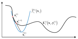
Figure 3: An illustration of stochastic successive convex approximation.

Similarly, in the $t$-th iteration, the $\left(2j\right)$-th block $\mathbf{y}_{j}$ is updated by solving the following subproblem:

$$\begin{split}\mathcal{P}_{y_{j}}:\mathop{\min}\limits_{\mathbf{y}_{j}}&\boldsymbol{L}_{j}^{\left(t\right)}\left(\mathbf{x}_{j}^{\left(t+1\right)},\mathbf{y}_{j}\right)\\ \text{s.t.}\quad&\sum\limits_{p=1}^{N_{p}}y_{j,p}=1,\quad\epsilon\leq y_{j,p}\leq 1,\quad\forall p.\end{split}$$

In stead of solving $\mathcal{P}_{y_{j}}$ directly, we first construct a simple quadratic surrogate objective function

$$\overline{f}_{y_{j}}^{\left(t\right)}\left(\mathbf{y}_{j}\right)\triangleq\left(\mathbf{\boldsymbol{{\rm f}}}_{y_{j}}^{\left(t\right)}\right)^{T}\left(\mathbf{y}_{j}-\mathbf{y}_{j}^{\left(t\right)}\right)+\varGamma_{y_{j}}\left\|\mathbf{y}_{j}-\mathbf{y}_{j}^{\left(t\right)}\right\|^{2},$$ (29)

and obtain an intermediate variable $\overline{\mathbf{y}}_{j}^{\left(t\right)}$ by minimizing the surrogate objective function as

$$\overline{\mathbf{y}}_{j}^{\left(t\right)} =\arg\min\overline{f}_{y_{j}}^{\left(t\right)}\left(\mathbf{y}_{j}\right)$$ (30)

$$s.t. \quad\sum\limits_{p=1}^{N_{p}}y_{j,p}=1,\quad\epsilon\leq y_{j,p}\leq 1,\quad\forall p,$$

where $\varGamma_{y_{j}}$ can be any positive number, $\mathbf{\boldsymbol{{\rm f}}}_{y_{j}}^{\left(t\right)}$ is an unbiased estimator of the gradient $\nabla_{\mathbf{y}_{j}}\boldsymbol{L}_{j}^{\left(t\right)}\left(\mathbf{x}_{j}^{\left(t+1\right)},\mathbf{y}_{j}^{\left(t\right)}\right)$, which is updated recursively as follows

$$\begin{split}\mathbf{\boldsymbol{{\rm f}}}_{y_{j}}^{\left(t\right)}&=\left(1-\rho^{\left(t\right)}\right)\mathbf{\boldsymbol{{\rm f}}}_{y_{j}}^{\left(t-1\right)}+\frac{\rho^{\left(t\right)}}{B}\sum_{b=1}^{B}\nabla_{\mathbf{y}_{j}}g_{j}^{\left(t\right)}\left(\mathbf{x}_{j}^{\left(t+1\right)},\mathbf{y}_{j}^{\left(t\right)};\boldsymbol{\Lambda}_{\sim j}^{\left(b\right)}\right)\end{split}$$ (31)

and we set $\mathbf{\boldsymbol{{\rm f}}}_{y_{j}}^{\left(-1\right)}=\boldsymbol{0}$. Finally, the updated $\mathbf{y}_{j}$ is given by

$$\mathbf{y}_{j}^{\left(t+1\right)}=\left(1-\gamma^{\left(t\right)}\right)\mathbf{y}_{j}^{\left(t\right)}+\gamma^{\left(t\right)}\overline{\mathbf{y}}_{j}^{\left(t\right)}.$$ (32)

To ensure the convergence of the algorithm, the step sizes $\rho^{\left(t\right)}$ and $\gamma^{\left(t\right)}$ must satisfy the following conditions.

Assumption 1 (Assumptions on step sizes).

 

1. $\rho^{t}\rightarrow 0$, $\sum_{t}\rho^{t}=\infty$, $\sum_{t}\left(\rho^{t}\right)^{2}<\infty$,

2. $\underset{t\rightarrow\infty}{\lim}\gamma^{t}/\rho^{t}=0$.

A typical choice of $\rho^{t},\gamma^{t}$ that satisfies Assumption 1 is $\rho^{t}=\mathcal{O}\left(t^{-\kappa_{1}}\right)$, $\gamma^{t}=\mathcal{O}\left(t^{-\kappa_{2}}\right)$, where $0.5<\kappa_{1}<\kappa_{2}\leq 1$. Such form of step sizes have been widely considered in stochastic optimization [30].

As can be seen, the surrogate optimization problems in (25) and (30) are quadratic programming with linear constraints, which is easy to solve. In addition, explicit expressions of the gradient $\nabla_{\mathbf{x}_{j}}g_{j}^{\left(t\right)}\left(\mathbf{x}_{j},\mathbf{y}_{j},\boldsymbol{\Lambda}_{\sim j}^{b}\right)$ and $\nabla_{\mathbf{y}_{j}}g_{j}^{\left(t\right)}\left(\mathbf{x}_{j},\mathbf{y}_{j},\boldsymbol{\Lambda}_{\sim j}^{b}\right)$ in (26) and (31) are given in the Appendix -C and -D, respectively.

The proposed SPVBI is guaranteed to converge to stationary points of the original Problem $\mathcal{P}_{2}$, as will be proved in Section IV-C. After the convergence, the corresponding discrete distribution of each variable $q\left(\boldsymbol{\Lambda}_{j}\right)$ composed of particles will approximate the marginal posteriori probability distribution, as illustrated in Fig. 2. As a result, we can take the particle position with the highest probability or the weighted sum of the particles as the final estimate, which are the approximate MAP estimate and MMSE estimate, respectively.

IV-C Convergence Analysis

In this section, we will prove the convergence of the SPVBI algorithm. First, we present a key lemma which gives some important properties of the surrogate functions.

Lemma 2 (Properties of the surrogate functions).

For each iteration $t=1,2,\ldots$ and each block $\mathbf{x}_{j},\mathbf{y}_{j},j=1,2,\ldots J$, we have

1. $\overline{f}_{x_{j}}^{\left(t\right)}\left(\mathbf{x}_{j}\right)$ and $\overline{f}_{y_{j}}^{\left(t\right)}\left(\mathbf{y}_{j}\right)$ are uniformly strongly convex in $\mathbf{x}_{j}$ and $\mathbf{y}_{j}$, respectively.

2. For any $\mathbf{x}_{j}\in\mathcal{X}$ and $\mathbf{y}_{j}\in\mathcal{Y}$, the function $\overline{f}_{x_{j}}^{\left(t\right)}\left(\mathbf{x}_{j}\right)$ and $\overline{f}_{y_{j}}^{\left(t\right)}\left(\mathbf{y}_{j}\right)$, their derivative, and their second order derivative are uniformly bounded.

3. $\overline{f}_{x_{j}}^{\left(t\right)}\left(\mathbf{x}_{j}\right)$ and $\overline{f}_{y_{j}}^{\left(t\right)}\left(\mathbf{y}_{j}\right)$ are Lipschitz continuous function w.r.t. $\mathbf{x}_{j}$ and $\mathbf{y}_{j}$, respectively. Moreover,

   $$\limsup_{t_{1},t_{2}\rightarrow\infty}\left|\overline{f}_{x_{j}}^{\left(t_{1}\right)}\left(\mathbf{x}_{j}\right)-\overline{f}_{x_{j}}^{\left(t_{2}\right)}\left(\mathbf{x}_{j}\right)\right|\leq B_{x}\left\|\mathbf{x}^{\left(t_{1}\right)}-\mathbf{x}^{\left(t_{2}\right)}\right\|,$$ (33)

   $$\limsup_{t_{1},t_{2}\rightarrow\infty}\left|\overline{f}_{y_{j}}^{\left(t_{1}\right)}\left(\mathbf{y}_{j}\right)-\overline{f}_{y_{j}}^{\left(t_{2}\right)}\left(\mathbf{y}_{j}\right)\right|\leq B_{y}\left\|\mathbf{y}^{\left(t_{1}\right)}-\mathbf{y}^{\left(t_{2}\right)}\right\|,$$ (34)

   $\forall\mathbf{x}_{j}\in\mathcal{X}$, $\forall\mathbf{y}_{j}\in\mathcal{Y}$, for some constants $B_{x}>0$ and $B_{y}>0$.

4. Consider a subsequence $\left\{\mathbf{x}^{\left(t_{i}\right)},\mathbf{y}^{\left(t_{i}\right)}\right\}_{i=1}^{\infty}$ converging to a limit point $\boldsymbol{x}^{*},\mathbf{y}^{*}$. There exist uniformly differentiable functions $\hat{f}_{x_{j}}\left(\mathbf{x}_{j}\right)$ and $\hat{f}_{y_{j}}\left(\mathbf{y}_{j}\right)$ such that

   $$\mathop{\lim}\limits_{i\to\infty}\overline{f}_{x_{j}}^{\left(t_{i}\right)}\left(\mathbf{x}_{j}\right)=\hat{f}_{x_{j}}\left(\mathbf{x}_{j}\right),\forall\mathbf{x}_{j}\in\mathcal{X},$$ (35)

   $$\mathop{\lim}\limits_{i\to\infty}\overline{f}_{y_{j}}^{\left(t_{i}\right)}\left(\mathbf{y}_{j}\right)=\hat{f}_{y_{j}}\left(\mathbf{y}_{j}\right),\forall\mathbf{y}_{j}\in\mathcal{Y}.$$ (36)

   Moreover, we have

   $$\left\|\nabla_{\mathbf{x}_{j}}\hat{f}_{x_{j}}\left(\mathbf{x}_{j}^{*}\right)-\nabla_{\mathbf{x}_{j}}L\left(\mathbf{x}^{*},\mathbf{y}^{*}\right)\right\|=0,$$ (37)

   $$\left\|\nabla_{\mathbf{y}_{j}}\hat{f}_{y_{j}}\left(\mathbf{y}_{j}^{*}\right)-\nabla_{\mathbf{y}_{j}}L\left(\mathbf{x}^{*},\mathbf{y}^{*}\right)\right\| =0.$$ (38)

Please refer to Appendix -A for the proof. With the Lemma 2, we are ready to prove the following main convergence result.

Theorem 3 (Convergence of SPVBI).

Starting from a feasible initial point $\mathbf{x}^{\left(0\right)},\mathbf{y}^{\left(0\right)}$, let $\left\{\mathbf{x}^{\left(t\right)},\mathbf{y}^{\left(t\right)}\right\}_{t=1}^{\infty}$ denote the iterates generated by Algorithm 2. Then every limiting point $\boldsymbol{x}^{*},\mathbf{y}^{*}$ of $\left\{\mathbf{x}^{\left(t\right)},\mathbf{y}^{\left(t\right)}\right\}_{t=1}^{\infty}$ is a stationary point of optimization problem $\mathcal{P}$ almost surely.

Please refer to Appendix -B for the proof.

IV-D Summary of the SPVBI Algorithm

The overall SPVBI algorithm is summarized in Algorithm 2. The mini-batch size $B$ can be chosen to achieve a trade-off between the per-iteration complexity and the total number of iterations. Thanks to the idea of averaging over iterations as in (26), (27), (31) and (32), a constant value of the mini-batch size $B$ is usually sufficient to achieve a fast convergence, e.g., in the simulations, we set $B=10$. Compared to the conventional PVBI algorithm which needs to calculate a summation of $N_{p}^{J-1}$ terms when updating one block in each iteration, the proposed SPVBI only requires to solve a simple quadratic programming problem which only involves the calculation of $B$ gradients, where $B$ can be much smaller than $N_{p}^{J-1}$. Moreover, the addition of updating particle position allows the algorithm to converge more quickly and flexibly to stable solutions. As such, the proposed SPVBI algorithm has both lower per-iteration complexity and faster convergence speed than the conventional PVBI.

The proposed SPVBI can be viewed as an extension of the SSCA framework [15] in terms of block-wise updating and control-dependent random state. First, the SSCA in [15] constructs a single surrogate function to update all the variables simultaneously in each iteration, while the SPVBI allows block-wise update, which is often used in VBI-type algorithms due to that a proper block partition facilitates algorithm derivation and possibly faster convergence [27]. Second, the distribution of the random state in the original SSCA framework is assumed to be independent of the optimization variable, i.e., is control independent, while the distribution of the random state in the SPVBI is control dependent. For example, the random state $\boldsymbol{\Lambda}_{{\rm\sim}j}$ in the $t$-th iteration follows the distribution $\prod_{j^{{}^{\prime}}\neq j}q\left(\boldsymbol{\Lambda}_{j^{{}^{\prime}}};\mathbf{x}_{j^{{}^{\prime}}},\mathbf{y}_{j^{{}^{\prime}}}\right)$, which depends on the value of the current optimization variables and is changing over iterations. Nevertheless, convergence can still be guaranteed.

Algorithm 2 Stochastic Particle-based VBI Algorithm

Input: received signals $\boldsymbol{r}$, multi-band frequency settings, the estimated number of scattering paths $\hat{K}$, $p\left(\hat{\boldsymbol{\Lambda}}\right)$, $\left\{\rho^{\left(t\right)},\gamma^{\left(t\right)}\right\}$.

Initialization: $\left\{x_{j,p}^{\left(0\right)}\backsim p\left(\hat{\boldsymbol{\Lambda}}_{j}\right),y_{j,p}^{\left(0\right)}=\frac{1}{N_{p}}\right\}_{p=1}^{N_{p}},\forall j$.

While not converge do $(t\rightarrow$$\infty)$

      For $j=1:J$

         Generate a mini-batch of realization based on the

         $\left\{x_{i,p},y_{i,p}\right\}_{p=1}^{N_{p}},i\neq j$;

         Update $\mathbf{\boldsymbol{{\rm f}}}_{x_{j}}^{\left(t\right)}$ or $\mathbf{\boldsymbol{{\rm f}}}_{y_{j}}^{\left(t\right)}$;

         Solving surrogate optimization problem $\mathcal{P}_{x_{j}}$ or $\mathcal{P}_{y_{j}}$;

         Update the particle position and weight of variable $\boldsymbol{\Lambda}_{j}$;

      end

end

Output: Find the position $\tilde{x}_{j},j=1,2,\ldots J$ of the particle with the maximum weight $y_{j}^{\left(max\right)}$. (i.e. MAP estimation)

V Numerical Simulation and Performance Analysis

In this section, simulations are conducted to demonstrate the performance of the proposed algorithm. We compare the proposed algorithm with the following baseline algorithms:

1. Baseline 1 (Root-MUSIC, R-MUSIC) [24]: The conventional root MUSIC algorithm has relatively high accuracy in delay estimation, so it is adopted here for single-band data, mainly to show the gain brought by combining the results of multiple bands.

2. Baseline 2 (Weighted Root-MUSIC, WR-MUSIC) [7]: The WR-MUSIC algorithm is adopted in the coarse estimation stage. See Section III-A for relevant procedures.

3. Baseline 3 (Spectral Estimation, SE) [24]: The parameters of the approximate all-pole model are estimated by spectral search methods such as root MUSIC algorithm, and the unknown frequency band data is interpolated according to the model to improve the resolution.

4. Baseline 4 (Sparse Bayesian Learning, SBL) [31]: The information required for coherent compensation can be extracted from the SBL solution. Then, by interpolating data between non-contiguous bands, more accurate estimate can be obtained, where the number of atoms $M_{ob}$ in the dictionary is set to be $2000$.

In the proposed SPVBI, each variable is equipped with $10$ particles, and the size of mini-batch $B$ is $10$. The step size sequence is set as follows: $\rho^{\left(t\right)}=5/\left(5+t\right)^{0.9},\rho^{\left(0\right)}=1$; $\gamma^{\left(t\right)}=5/\left(15+t\right)^{1},\gamma^{\left(0\right)}=1$. Unless otherwise specified, the experiment was repeated $400$ times.

In the simulations, we consider both small-bandwidth and large-bandwidth scenarios, which can cover common WiFi applications such as localization and imaging. We first describe the common setup for both scenarios. There are two scattering paths. The amplitude of $\alpha_{k}$ is $1$ and $0.5$, and $\beta_{k}$ is $-\pi/4$ and $\pi/4$, respectively. In addition, the phase of $\alpha_{k}$ and initial phase $\phi_{m}$ are uniformly generated within $[0,2\pi]$. The subcarrier spacing is $78.125$KHz.

In the small-bandwidth scenario, the received signals come from two non-adjacent frequency bands with a bandwidth of $40$MHz. The initial frequency is set to $2.4$GHz and $2.52$GHz, respectively. There are two scattering paths with delays of $25$ns and $500$ns. The timing synchronization error $\delta_{m}$ is generated following a Gaussian distribution $\mathcal{N}\left(0,0.01\text{ns}^{2}\right)$.

In the large-bandwidth scenario, the bandwidth of the two non-contiguous frequency bands is $320$MHz. The initial frequency is set to $5$GHz and $6$GHz, respectively. The delays of the two scattering paths are $10$ns and $20$ns, respectively. The timing synchronization error $\delta_{m}$ is generated following a Gaussian distribution $\mathcal{N}\left(0,1\text{ns}^{2}\right)$.

V-A Performance Comparison with Conventional PVBI Algorithm

In this section, we will compare the performance of the proposed SPVBI algorithm with that of the conventional PVBI algorithm.

Firstly, we will focus on the convergence performance. The benefits of updating particle positions are first shown by comparing the proposed SPVBI with and without updating particle positions (i.e., PVBI).

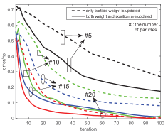
Figure 4: Iteration error curves with different particle numbers.

In Fig. 4, we plot the convergence curves of different updating modes with different number of particles under the small-bandwidth setup. As the number of particles decreases from $20$ to $5$, it can be seen that the convergence speed will slow down when only the weight is updated, but the convergence speed and performance will almost remain the same when the position is also updated. This means that updating the position of particles can effectively increase the degree of freedom of optimization and ensure convergence and performance even with fewer particles.

Secondly, we will focus on the estimation accuracy performance. As mentioned in the above, due to the large number of variables in multi-band WiFi sensing scenarios, PVBI algorithms with excessive computational complexity are not applicable. Therefore, we consider a simplified case to compare the performance of SPVBI, PVBI, and other algorithms, where there is only one major scattering center with delay of $50$ns, and there is no imperfect factors. The SNR is $12$dB, the amplitude of $\alpha_{1}$ is $1$ and $\beta_{1}$ is $-\pi/4$. The initial frequencies of the two non-adjacent bands are $2.4$GHz and $2.94$GHz, respectively, and the bandwidth as well as the frequency step are $40$MHz and $78.125$KHz, respectively.

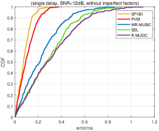
Figure 5: Performance comparison of the algorithms in a simplified case.

From the error cumulative distribution function (CDF) curve of the time delay shown in Fig. 5, it can be seen that SPVBI performs better than the conventional PVBI, because it additionally update the position of the particle, so that the particles have a higher degree of freedom to approximate the posteriori probability. Moreover, the performance of SPVBI and PVBI algorithms is better than that of the other algorithms, because these two VBI-based algorithms can take advantage of the performance gain brought by multi-band.

In the following, we further consider more general scenarios with multipath and imperfect factors The detailed parameter settings are listed at the beginning of Section V.

V-B Target Parameter Estimation Error

In small-bandwidth positioning scenarios, our primary concern is the distance/range of a certain target. Therefore, we need to investigate the average delay estimation error and the various factors that can affect it.

Impact of the SNR

In Fig. 6, it can be seen that the performance of all algorithms improves as the SNR increases from $5$dB to $20$dB. At a certain SNR, the root-mean-square error (RMSE) of SPVBI is closer to the CRB and significantly lower than that of other algorithms, indicating higher time delay estimation accuracy. The performance of the SBL algorithm for delay estimation is inferior to WR-MUSIC, even when the dictionary size is already quite large (i.e. $2000$ atoms).

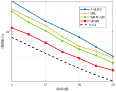
Figure 6: RMSE of delay estimation with respect to the SNR.

Impact of the band gap

This subsection presents the impact of the band gap. We changed the initial frequency of the second band from $2.4$GHz to $2.52$GHz in steps of $40$MHz to investigate the performance change of the SPVBI algorithm.

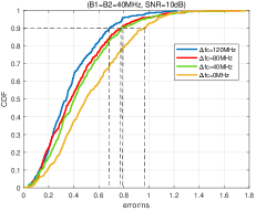
Figure 7: CDF curves of delay estimation errors for different band gap.

In Fig. 7, with the increase of frequency band gap, the performance of SPVBI algorithm keeps improving, which indicates that the proposed algorithm does utilize the multi-band gap aperture gain. Intuitively, the larger the frequency band gap, the more obvious the phase rotation caused by the same delay, which means that the minor delay variation can also be captured, and hence the better performance.

V-C Resolution Performance

In the application scenarios of large-bandwidth WiFi, such as WiFi imaging and target feature extraction, ultra-high resolution is required. In this case, it is often desirable to reconstruct the full-band data from the available non-adjacent band data to improve the resolution.

However, whether high resolution can be achieved will depend on the accuracy of the data reconstruction. Therefore, for the SPVBI algorithm and Baseline $3$ and $4$, we compare the RMSE of data reconstruction to indirectly show the resolution performance.

The RMSE between the estimated full-band data and the true full-band data can be calculated via the following equation: $RMSE_{data}=\sqrt{\frac{1}{N}\sum_{n=1}^{N}\left|r^{\left(n\right)}-\hat{r}^{\left(n\right)}\right|^{2}}$, where $N$ indicates the number of subcarriers in the full-band.

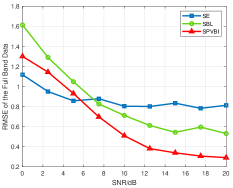
Figure 8: RMSE of data reconstruction under different SNR.

In Fig. 8, we show the RMSE of full-band data reconstruction under different SNR. In the case of low SNR, SE algorithm is less affected by noise due to its simple model and few parameters to be estimated. However, with the increase of SNR, compared with other multi-band fusion algorithms, the full-band data reconstructed by SPVBI is more accurate, which implies that the proposed algorithm can obtain more accurate estimation of the signal parameters. The RMSE performance of SBL algorithm is worse than that of SPVBI and its complexity is higher.

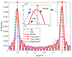
Figure 9: High resolution range profile (12dB).

In addition, Fig. 9 shows the high resolution range profile (HRRP) reconstructed by full-band data of different algorithms. It can be found that the HRRP of the multi-band fusion algorithm (i.e. SE, SBL, SPVBI) is narrower than that of the single-band reconstruction, so the resolution is higher. Meanwhile, the RMSE of the full-band data reconstructed by SPVBI algorithm is smaller, so the peak point of SPVBI is closer to the true value as shown in the rectangular box.

V-D Sensitivity Analysis of the Number of Scattering Paths

In this subsection, we will focus on the impact of missed detection and false alarm on the performance for our algorithm, which often occur in the detection phase and bring the risk of degradation.

Fig. 10 demonstrates the sensitivity of our algorithm to incorrect paths number at $SNR=10$dB. The red curve represents the performance of estimating the first path delay when the exact number is known. The blue and green curve depict cases in which the path-2 is missed and the false path-3 is detected, respectively. The amplitudes of $\alpha_{k}$ are $1$ and $0.3$, respectively. The remaining parameters are the same as in the default simulation setup in the small-bandwidth scenario.

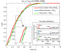
Figure 10: Impact of the multipath misdetection on the performance of SPVBI.

As shown in Fig. 10, both missed detection and false alarm do not significantly degrade the performance of estimating the first path delay. This indicates that our algorithm is not highly sensitive to mismatch in the number of scattering paths.

V-E Analysis and Comparison of Computational Complexity

In this subsection, our focus will be on analyzing the complexity of the different algorithms and presenting the complexity results of them.

For Root-MUSIC (R-MUSIC) [22, 24] algorithm, it mainly includes subspace decomposition and polynomial rooting, with the complexity of $\mathcal{O}\left(MN_{m}^{3}\right)$ and $\mathcal{O}\left(M\left(2N_{m}-1\right)^{3}\right)$, respectively. $M$ is the number of frequency bands and $N_{m}$ denotes the number of subcarriers in each band. For multi-band weighted root-MUSIC (WR-MUSIC) algorithm [7], the complexity is about $M$ times that of R-MUSIC algorithm. In addition, the computational complexity of least square (LS) method in the coarse estimation stage is approximately $\mathcal{O}\left(N_{m}K^{2}+K^{3}\right)$, which is negligible compared with WR-MUSIC. $K$ is the number of scattering paths. For SE algorithm [24], in addition to the R-MUSIC algorithm used separately for each band, there is a nonlinear least square fitting step, which is solved by Levenberg-Marquarelt (LM) algorithm with a complexity order of $\mathcal{O}\left(N_{m}^{3}\right)$. Therefore, the total computational complexity of SE algorithm is $M\cdot\mathcal{O}_{R-MUSIC}+\mathcal{O}\left(N_{m}^{3}\right)$. For SBL algorithm [31], the main cost depends on the size of the observation matrix used, with a complexity order of $\mathcal{O}\left(M\cdot M_{ob}^{3}\right)$, $M_{ob}$ is the number of atoms.

For PVBI algorithm, its per-iteration complexity order is $\mathcal{O}\left(J\cdot\left(N_{p}\right)^{J-1}N_{LH}\right)$, where $N_{LH}=\mathcal{O}\left(KMN_{m}\right)$ represents the average number of floating point operations (FLOPs) required to compute the dominant logarithmic likelihood value. For SPVBI algorithm, through mini-batch sampling and minimization of quadratic surrogate objective functions, the per-iteration complexity can be reduced to $\mathcal{O}\left(2J\cdot\left(N_{p}BN_{grad}+N_{p}^{3}\right)\right)$, where $BN_{grad}$ and $N_{p}^{3}$ represent the complexity of computing a mini-batch of gradients and quadratic programming search, respectively, where $N_{grad}=\mathcal{O}\left(KMN_{m}\right)$ represents the average number of FLOPs required to compute a gradient. It can be seen that SPVBI greatly reduces the computational complexity compared with conventional PVBI.

In Table II, we summarize the per-iteration complexity order of different algorithms, and numerically compare them under a typical setting as follows: $J=8$, $N_{p}=10$, $M=2$, $N_{m}=256$, $B=10$, $N_{LH}=20000$, $N_{grad}=18000$, $M_{ob}=2000$.

TABLE II: COMPARISON OF THE COMPLEXITY ORDER FOR DIFFERENT ALGORITHMS.

Algorithms	Complexity order per iteration	Typical values
PVBI	$\mathcal{O}\left(J\cdot\left(N_{p}\right)^{J-1}\cdot N_{LH}\right)$	$1.56\times 10^{12}$
SPVBI	$\mathcal{O}\left(2J\cdot\left(N_{p}BN_{grad}+N_{p}^{3}\right)\right)$	$2.88\times 10^{7}$
R-MUSIC	$\mathcal{O}\left(N_{m}^{3}+\left(2N_{m}-1\right)^{3}\right)$	$1.50\times 10^{8}$
WR-MUSIC	$\mathcal{O}\left(MN_{m}^{3}+M\left(2N_{m}-1\right)^{3}\right)$	$3.00\times 10^{8}$
SE	$M\cdot\mathcal{O}_{R-MUSIC}+\mathcal{O}\left(N_{m}^{3}\right)$	$3.17\times 10^{8}$
SBL	$\mathcal{O}\left(M\cdot M_{ob}^{3}\right)$	$1.60\times 10^{10}$

It can be found that SPVBI algorithm can achieve good trade-off between performance and complexity. PVBI algorithm can only be applied in scenarios with few variables, and once the number of variables is large, the complexity will be unacceptable. Although the computational complexity of two-stage estimation (i.e. $\mathcal{O}_{WR-MUSIC}+\mathcal{O}_{SPVBI}$) is higher than that of the WR-MUSIC and SE algorithm, the estimation accuracy and resolution are greatly improved. Compared with the SBL algorithm, the complexity of SPVBI is greatly reduced and the performance is also improved.

VI Conclusions

In this paper, we proposed a novel two-stage design for multi-band WiFi sensing. To overcome the difficulty caused by the oscillation of likelihood function, we adopt two distinct signal models, which are transformed from the original multi-band signal model and used within a two-stage estimation framework. The coarse estimation stage helps to reduce the computational complexity by narrowing down the estimation range, and the refined estimation stage leverages the carrier phase information between different frequency bands (i.e., multi-band gap gain) to improve estimation performance further. Moreover, the SPVBI algorithm based on block SSCA transforms the computation of expectation with exponential complexity in the conventional PVBI into solving stochastic optimization problems, guaranteeing convergence theoretically and reducing computational complexity through mini-batch random sampling and averaging over iterations. Simulation results indicate that the proposed algorithm achieves good performance with acceptable complexity across different scenarios. Moreover, adding the particle position update can speed up convergence and reduce the required number of particles. It is worth mentioning that the proposed framework has good generalization ability, and is expected to be applied to more high-dimensional non-convex parameter estimation scenarios with numerous local optimums and non-conjugated prior. In the future, other more expressive methods to characterize the posterior distribution and the combination with artificial intelligence can also be further explored.

-A Proof of Lemma 2

We first introduce the following preliminary result.

Lemma 4.

Given subproblem $\mathcal{P}_{x_{j}}$ and $\mathcal{P}_{y_{j}}$ under Lemma 2, suppose that the step sizes $\rho^{t}$and $\gamma^{t}$ are chosen according to Assumption 1. Let $\left\{\mathbf{x}^{\left(t\right)},\mathbf{y}^{\left(t\right)}\right\}$ be the sequence generated by Algorithm 2. Then, the following holds

$$\mathop{\lim}\limits_{t\to\infty}\left|\mathbf{\boldsymbol{{\rm f}}}_{x_{j}}^{\left(t\right)}-\nabla_{\mathbf{x}_{j}}\boldsymbol{L}_{j}^{\left(t\right)}\left(\mathbf{x}_{j}^{\left(t\right)},\mathbf{y}_{j}^{\left(t\right)}\right)\right|=0,w.p.1.$$ (39)

$$\mathop{\lim}\limits_{t\to\infty}\left|\mathbf{\boldsymbol{{\rm f}}}_{y_{j}}^{\left(t\right)}-\nabla_{\mathbf{y}_{j}}\boldsymbol{L}_{j}^{\left(t\right)}\left(\mathbf{x}_{j}^{\left(t+1\right)},\mathbf{y}_{j}^{\left(t\right)}\right)\right|=0.w.p.1.$$ (40)

Proof:

Lemma 4 is a consequence of ([32], Lemma 1). We only need to verify that all the technical conditions therein are satisfied. Specifically, Condition (a) of ([32], Lemma 1) is satisfied because $\mathcal{X}$ and $\mathcal{Y}$ are compact and bounded. Condition (b) of ([32], Lemma 1) follows from the boundedness of the instantaneous gradient $\nabla g_{j}^{\left(t\right)}$. Conditions (c)–(d) immediately come from the step-size rule (1) in Assumption 1. Although the control-dependent random states are not identically distributed over iterations, the distributions (i.e., positions and weights of particles) change slowly at the rate of order $\mathcal{O}\left(\gamma^{t}\right)$, so we have $\left\|\nabla\boldsymbol{L}_{j}^{\left(t+1\right)}-\nabla\boldsymbol{L}_{j}^{\left(t\right)}\right\|=\mathcal{O}\left(\gamma^{t}\right)$. Plusing the step-size rule 2) in Assumption 1, Condition (e) of ([32], Lemma 1) is also satisfied. ∎

Using this result, since $\nabla\boldsymbol{L}_{j}^{\left(t\right)}\left(\mathbf{x}_{j}^{\left(t\right)},\mathbf{y}_{j}^{\left(t\right)}\right)$ is obviously bounded, then $\mathbf{\boldsymbol{{\rm f}}}_{x_{j}}^{\left(t\right)}$ and $\mathbf{\boldsymbol{{\rm f}}}_{y_{j}}^{\left(t\right)}$ are bounded. As can be seen, the surrogate function adopted is a convex quadratic function with box constraints. Therefore, 1)-3) in Lemma 2 follow directly from the expression of the surrogate function in (24) and (29).

For 4) in Lemma 2, the proof is similar to that of ([15], Lemma 1). Due to 1)-3) in Lemma 2, the families of functions $\left\{\overline{f}_{x_{j}}^{\left(t_{i}\right)}\left(\mathbf{x}_{j}\right)\right\}$ and $\left\{\overline{f}_{y_{j}}^{\left(t_{i}\right)}\left(\mathbf{y}_{j}\right)\right\}$ are equicontinuous. Moreover, they are bounded and defined over a compact set $\mathcal{X}$ and $\mathcal{Y}$. Hence the Arzela–Ascoli theorem [33] implies that, by restricting to a subsequence, there exists uniformly continuous functions $\hat{f}_{x_{j}}\left(\mathbf{x}_{j}\right)$ and $\hat{f}_{y_{j}}\left(\mathbf{y}_{j}\right)$ such that (35) and (36) in Lemma 2-4) are satisfied. Clearly, we have

$$\nabla_{\mathbf{x}_{j}/\mathbf{y}_{j}}\boldsymbol{L}\left(\mathbf{x}^{*},\mathbf{y}^{*}\right)=\nabla_{\mathbf{x}_{j}/\mathbf{y}_{j}}\boldsymbol{L}_{j}\left(\mathbf{x}^{*},\mathbf{y}^{*}\right)$$ (41)

almost surely. And because of $\mathop{\lim}\limits_{i\to\infty}\mathbf{\boldsymbol{{\rm f}}}_{x_{j}}^{\left(t_{i}\right)}=\nabla_{\mathbf{x}_{j}}\hat{f}_{x_{j}}\left(\mathbf{x}_{j}^{*}\right)$, $\mathop{\lim}\limits_{i\to\infty}\mathbf{\boldsymbol{{\rm f}}}_{y_{j}}^{\left(t_{i}\right)}=\nabla_{\mathbf{y}_{j}}\hat{f}_{y_{j}}\left(\mathbf{y}_{j}^{*}\right)$ and Lemma 4, we further have

$$\left\|\nabla_{\mathbf{x}_{j}}\hat{f}_{x_{j}}\left(\mathbf{x}_{j}^{*}\right)-\nabla_{\mathbf{x}_{j}}\boldsymbol{L}\left(\mathbf{x}^{*},\mathbf{y}^{*}\right)\right\| =0,$$ (42)

$$\left\|\nabla_{\mathbf{y}_{j}}\hat{f}_{y_{j}}\left(\mathbf{y}_{j}^{*}\right)-\nabla_{\mathbf{y}_{j}}\boldsymbol{L}\left(\mathbf{x}^{*},\mathbf{y}^{*}\right)\right\| =0.$$ (43)

-B Proof of Theorem 3

It is easy to see that each iteration of Algorithm 2 is equivalent to optimizing the following surrogate function

$$\overline{f}^{\left(t\right)}\left(\mathbf{x},\mathbf{y}\right)=\sum\limits_{j=1}^{J}\left[\overline{f}_{x_{j}}^{\left(t\right)}\left(\mathbf{x}_{j}\right)+\overline{f}_{y_{j}}^{\left(t\right)}\left(\mathbf{y}_{j}\right)\right].$$ (44)

Moreover, from Lemma 2, we have

$$\mathop{\lim}\limits_{t\to\infty}\overline{f}^{\left(t\right)}\left(\mathbf{x},\mathbf{y}\right)=\hat{f}\left(\mathbf{x},\mathbf{y}\right)\triangleq\sum\limits_{j=1}^{J}\left[\hat{f}_{x_{j}}\left(\mathbf{x}_{j}\right)+\hat{f}_{y_{j}}\left(\mathbf{y}_{j}\right)\right].$$ (45)

Using Lemma 2 and the similar analysis as in the proof of ([15], Theorem 1), we have that

$$\left\{\mathbf{x}^{*},\mathbf{y}^{*}\right\} =\arg\min\hat{f}\left(\mathbf{x},\mathbf{y}\right)$$

s.t.  $$h_{j}\left(\mathbf{x},\mathbf{y}\right)\leq \quad H_{j}\left(\mathbf{x},\mathbf{y}\right)=0,\quad j=1,\ldots,J$$0, (46)

where $h_{j}\left(\mathbf{x},\mathbf{y}\right)$ and $H_{j}\left(\mathbf{x},\mathbf{y}\right)$ represent inequality constraints and equality constraints in the original problem, respectively. The Karush-Kuhn-Tucker (KKT) condition of problem (46) implies that there exist $\lambda_{1},\ldots,\lambda_{J}$ and $\mu_{1},\ldots,\mu_{J}$ that

$$\nabla\hat{f}\left(\mathbf{x}^{*},\mathbf{y}^{*}\right)+\sum\limits_{j=1}^{J}\mu_{j}\nabla h_{j}\left(\mathbf{x}^{*},\mathbf{y}^{*}\right)+\sum\limits_{j=1}^{J}\lambda_{j}\nabla H_{j}\left(\mathbf{x}^{*},\mathbf{y}^{*}\right) =0$$

$$h_{j}\left(\mathbf{x}^{*},\mathbf{y}^{*}\right)\leq 0,\quad\quad H_{j}\left(\mathbf{x}^{*},\mathbf{y}^{*}\right)=0,\quad j=1,\ldots,J$$

$$\mu_{j}\geq 0,\quad\quad\mu_{j}h_{j}\left(\mathbf{x}^{*},\mathbf{y}^{*}\right)=0,\quad j=1,\ldots,J.$$ (47)

Finally, it follows from Lemma 2 and (47) that $\left\{\mathbf{x}^{*},\mathbf{y}^{*}\right\}$ also satisfies the KKT condition of Problem $\mathcal{P}$. This completes the proof.

-C Derivation of Particle Position Gradient

The general formula for the gradient of position is

$$\frac{\partial g_{j}^{\left(t\right)}\left(\mathbf{x}_{j}^{\left(t\right)},\mathbf{y}_{j}^{\left(t\right)},\boldsymbol{\Lambda}_{\sim j}^{\left(b\right)}\right)}{\partial x_{j,p}^{\left(t\right)}}$$

$$=-y_{j,p}^{\left(t\right)}\left[\frac{\partial\ln p\left(x_{j,p}^{\left(t\right)}\right)}{\partial x_{j,p}^{\left(t\right)}}+\frac{\partial\ln p\left(\boldsymbol{r}\left|\boldsymbol{\Lambda}_{\sim j}^{\left(b\right)},x_{j,p}^{\left(t\right)}\right.\right)}{\partial x_{j,p}^{\left(t\right)}}\right],$$ (48)

where the superscript $\left(b\right)$ indicates that its value is generated by the $b$-th sample of a mini-batch.

Without any additional priors, we assume that the variables are uniformly distributed in the interval, so the derivatives $\frac{\partial\ln p\left(x\right)}{\partial x}$ defined in the interval are all $0$. For the Gaussian prior $\mathcal{N}\left(0,var\right)$, the derivative is

$$\frac{\partial\ln p\left(x\right)}{\partial x}=\frac{p\left(x\right)}{p\left(x\right)}\left[\frac{-\left(x-0\right)}{var}\right]=-x/var.$$ (49)

Next, we will focus on the gradient of the likelihood function with respect to position:

$$\frac{\partial\ln p\left(\boldsymbol{r}\left|\boldsymbol{\Lambda}_{\sim j}^{\left(b\right)},x_{j,p}^{\left(t\right)}\right.\right)}{\partial x_{j,p}^{\left(t\right)}} =\frac{-1}{{\rm 2}\eta_{w}^{2}}\sum\limits_{m=1}^{M}\sum\limits_{n=0}^{N_{m}-1}\frac{\partial\left|r_{m}^{\left(n\right)}-s_{m}^{\left(n\right)}\right|^{2}}{\partial x_{j,p}^{\left(t\right)}}$$

$$=\frac{-1}{\eta_{w}^{2}}\sum\limits_{m=1}^{M}\sum\limits_{n=0}^{N_{m}-1} \left[Re\left(s_{m}^{\left(n\right)}-r_{m}^{\left(n\right)}\right)\frac{\partial Re\left(s_{m}^{\left(n\right)}\right)}{\partial x_{j,p}^{\left(t\right)}}\right.$$

$$+Im\left(s_{m}^{\left(n\right)}-r_{m}^{\left(n\right)}\right) \left.\frac{\partial Im\left(s_{m}^{\left(n\right)}\right)}{\partial x_{j,p}^{\left(t\right)}}\right],$$ (50)

where the terms $\frac{\partial Re\left(s_{m}^{\left(n\right)}\right)}{\partial x_{j,p}^{\left(t\right)}}$ and $\frac{\partial Im\left(s_{m}^{\left(n\right)}\right)}{\partial x_{j,p}^{\left(t\right)}}$ for different variables can be easily derived according to (5).

-D Derivation of Particle Weight Gradient

The general formula for the gradient of weight is

$$\frac{\partial g_{j}^{\left(t\right)}\left(\mathbf{x}_{j}^{\left(t+1\right)},\mathbf{y}_{j}^{\left(t\right)},\boldsymbol{\Lambda}_{\sim j}^{\left(b\right)}\right)}{\partial y_{j,p}^{\left(t\right)}}$$

$$=\ln y_{j,p}^{\left(t\right)}-\ln p\left(x_{j,p}^{\left(t+1\right)}\right)-\ln p\left(r\left|\boldsymbol{\Lambda}_{{\rm\sim}j}^{\left(b\right)},x_{j,p}^{\left(t+1\right)}\right.\right)+1.$$ (51)

References

- [1] F. Liu, Y. Cui, C. Masouros, J. Xu, T. X. Han, Y. C. Eldar, and S. Buzzi, “Integrated sensing and communications: Toward dual-functional wireless networks for 6g and beyond,” IEEE Journal on Selected Areas in Communications, vol. 40, no. 6, pp. 1728–1767, 2022.
- [2] C. Deng, X. Fang, X. Han, X. Wang, L. Yan, R. He, Y. Long, and Y. Guo, “IEEE 802.11be Wi-Fi 7: New challenges and opportunities,” IEEE Commun. Surveys Tuts., vol. 22, no. 4, pp. 2136–2166, 4th Quart. 2020.
- [3] T. Kazaz, G. J. M. Janssen, J. Romme, and A.-J. van der Veen, “Delay estimation for ranging and localization using multiband channel state information,” IEEE Trans. Wireless Commun., vol. 21, no. 4, pp. 2591–2607, Apr. 2022.
- [4] Y. Xie, Z. Li, and M. Li, “Precise power delay profiling with commodity Wi-Fi,” IEEE Trans. Mobile Comput., vol. 18, no. 6, pp. 1342–1355, Jun. 2019.
- [5] D. Vasisht, S. Kumar, and D. Katabi, “Decimeter-level localization with a single WiFi access point,” in Proc. 13th Conf. Netw. Syst. Design Implement. (NSDI), Mar. 2016, pp. 165–178.
- [6] T. Kazaz, R. T. Rajan, G. J. M. Janssen, and A.-J. v. der Veen, “Multiresolution time-of-arrival estimation from multiband radio channel measurements,” in Proc. IEEE Int. Conf. Acoust. Speech Signal Process., May. 2019, pp. 4395–4399.
- [7] M. Pourkhaatoun and S. A. Zekavat, “High-resolution low-complexity cognitive-radio-based multiband range estimation: Concatenated spectrum vs. fusion-based,” IEEE Systems Journal, vol. 8, no. 1, pp. 83–92, 2014.
- [8] J. Xiong, K. Sundaresan, and K. Jamieson, “ToneTrack: Leveraging frequency-agile radios for time-based indoor wireless localization,” in Proc. 21st Annu. Int. Conf. Mobile Comput. Netw. (MobiCom), Sep. 2015, pp. 537–549.
- [9] X. Li and K. Pahlavan, “Super-resolution TOA estimation with diversity for indoor geolocation,” IEEE Trans. Wireless Commun., vol. 3, no. 1, pp. 224–234, Jan. 2004.
- [10] M. B. Khalilsarai, S. Stefanatos, G. Wunder, and G. Caire, “WiFi-based indoor localization via multi-band splicing and phase retrieval,” in Proc. IEEE 20th Int. Workshop Signal Process. Adv. Wireless Commun. (SPAWC), Jul. 2019, pp. 1–5.
- [11] M. B. Khalilsarai, B. Gross, S. Stefanatos, G. Wunder, and G. Caire, “WiFi-based channel impulse response estimation and localization via multi-band splicing,” in Proc. IEEE Global Commun. Conf. (GLOBECOM), Dec. 2020, pp. 1–6.
- [12] T. Kazaz, M. Coutino, G. J. M. Janssen, and A.-J. van der Veen, “Joint blind calibration and time-delay estimation for multiband ranging,” in ICASSP 2020 - 2020 IEEE International Conference on Acoustics, Speech and Signal Processing (ICASSP), 2020, pp. 4846–4850.
- [13] B. H. Fleury, M. Tschudin, R. Heddergott, D. Dahlhaus, and K. I. Pedersen, “Channel parameter estimation in mobile radio environments using the sage algorithm,” IEEE Journal on Selected Areas in Communications, vol. 17, no. 3, pp. 434–450, 1999.
- [14] I. Ziskind and M. Wax, “Maximum likelihood localization of multiple sources by alternating projection,” IEEE Trans. Acoust. Speech Signal Processing, vol. 36, no. 10, pp. 1553–1560, Oct. 1988.
- [15] A. Liu, V. K. N. Lau, and B. Kananian, “Stochastic successive convex approximation for non-convex constrained stochastic optimization,” IEEE Transactions on Signal Processing, vol. 67, no. 16, pp. 4189–4203, 2019.
- [16] M. B. Khalilsarai, B. Gross, S. Stefanatos, G. Wunder, and G. Caire, “Wifi-based channel impulse response estimation and localization via multi-band splicing,” in GLOBECOM 2020 - 2020 IEEE Global Communications Conference, 2020, pp. 1–6.
- [17] A. T. Mariakakis, S. Sen, J. Lee, and K.-H. Kim, “Sail: Single access point-based indoor localization,” in Proc. 12th Annu. Int. Conf. Mobile Syst. Appl. Services, Jun. 2014, pp. 315–328. [Online]. Available: https://doi.org/10.1145/2594368.2594393
- [18] H. Xu and L. Yang, “Calibration of random phase rotation for multi-band OFDM UWB signals,” in Proc. 44th Asilomar Conf. Signals Syst. Comput., Nov. 2010, pp. 170–174.
- [19] T. Kazaz, G. J. M. Janssen, J. Romme, and A.-J. van der Veen, “Delay estimation for ranging and localization using multiband channel state information,” IEEE Transactions on Wireless Communications, vol. 21, no. 4, pp. 2591–2607, 2022.
- [20] M. Wax and T. Kailath, “Detection of signals by information theoretic criteria,” IEEE Transactions on Acoustics, Speech, and Signal Processing, vol. 33, no. 2, pp. 387–392, 1985.
- [21] M. Wax and I. Ziskind, “Detection of the number of coherent signals by the mdl principle,” IEEE Transactions on Acoustics, Speech, and Signal Processing, vol. 37, no. 8, pp. 1190–1196, 1989.
- [22] B. D. Rao and K. S. Hari, “Performance analysis of root-music,” IEEE Transactions on Acoustics, Speech, and Signal Processing, vol. 37, no. 12, pp. 1939–1949, 1989.
- [23] S. Y. Kung, K. S. Arun, and D. Rao, “State-space and singular-value decomposition-based approximation methods for the harmonic retrieval problem,” J.opt.soc.amer, vol. 73, no. 12, pp. 1799–1811, 1983.
- [24] K. Cuomo, J. Pion, and J. Mayhan, “Ultrawide-band coherent processing,” IEEE Transactions on Antennas and Propagation, vol. 47, no. 6, pp. 1094–1107, 1999.
- [25] C. W. Fox and S. J. Roberts, “A tutorial on variational bayesian inference,” Artificial Intelligence Review, vol. 38, no. 2, pp. 85–95, 2012.
- [26] M. J. Beal, “Variational algorithms for approximate bayesian inference,” Phd Thesis University of London, 2003.
- [27] B. Zhou, Q. Chen, H. Wymeersch, P. Xiao, and L. Zhao, “Variational inference-based positioning with nondeterministic measurement accuracies and reference location errors,” IEEE Transactions on Mobile Computing, vol. 16, no. 10, pp. 2955–2969, 2017.
- [28] M. Vemula, M. F. Bugallo, and P. M. Djuric, “Sensor self-localization with beacon position uncertainty,” Signal Processing, vol. 89, no. 6, pp. 1144–1154, 2009.
- [29] G. Parisi and R. Shankar, “Statistical field theory,” Physics Today, vol. 41, no. 12, p. 110, 1988.
- [30] Y. Yang, G. Scutari, D. P. Palomar, and M. Pesavento, “A parallel decomposition method for nonconvex stochastic multi-agent optimization problems,” IEEE Transactions on Signal Processing, vol. 64, no. 11, pp. 2949–2964, 2016.
- [31] H. H. Zhang and R. S. Chen, “Coherent processing and superresolution technique of multi-band radar data based on fast sparse bayesian learning algorithm,” IEEE Transactions on Antennas and Propagation, vol. 62, no. 12, pp. 6217–6227, 2014.
- [32] A. Ruszczynski, “Feasible direction methods for stochastic programming problems,” Mathematical Programming, vol. 19, no. 1, pp. 220–229, 1980.
- [33] N. Dunford and J. T. Schwartz, “Linear operators: Part 1 general theory,” Interscience Publishers, 1988.