The Forecast Trap

Abstract

Encouraged by decision makers’ appetite for future information on topics ranging from elections to pandemics, and enabled by the explosion of data and computational methods, model based forecasts have garnered increasing influence on a breadth of decisions in modern society. Using several classic examples from fisheries management, I demonstrate that selecting the model or models that produce the most accurate and precise forecast (measured by statistical scores) can sometimes lead to worse outcomes (measured by real-world objectives). This can create a forecast trap, in which the outcomes such as fish biomass or economic yield decline while the manager becomes increasingly convinced that these actions are consistent with the best models and data available. The forecast trap is not unique to this example, but a fundamental consequence of non-uniqueness of models. Existing practices promoting a broader set of models are the best way to avoid the trap.

Global change issues are complex and outcomes are difficult to predict (Clark et al. 2001). To guide decisions in an uncertain world, researchers and decision makers may consider a range of alternative plausible models to better reflect what we do and do not know about the processes involved (Polasky et al. 2011). Forecasts or predictions from possible models can indicate what outcomes are most likely to result under what decisions or actions. This has made model-based forecasts a cornerstone for scientifically based decision making. By comparing outcomes predicted by a model to future observations, a decision maker can not only plan for the uncertainty, but also learn which models are most trustworthy. The value of iterative learning has long been reflected in the theory of adaptive management (Walters & Hilborn 1978) as well as in actual adaptive management practices such as Management Strategy Evaluation (MSE) (Punt et al. 2016) used in fisheries, and is a central tenet of a rapidly growing interest in ecological forecasting (Dietze et al. 2018). But, do iterative learning approaches always lead to better decisions?

In this paper, I demonstrate that the model that makes the better prediction (defined as a strictly proper score, Gneiting & Raftery (2007)) is not necessarily the model that makes the better policy (defined in terms of utility, e.g. expected net present value, Clark (1990)). I show that our best methods for learning about model structure or parameters by repeatedly comparing forecasts to observations can be counter-productive. Put another way, the value of information (VOI, as measured by the expected utility given that information minus the utility without it; see Howard (1966); Katz et al. (1987)), can actually be negative. When VOI is negative, the decision-maker may become trapped into accepting mediocre outcomes derived from a model that makes accurate forecasts, even when a less accurate model that would generate better outcomes is available. This trap is invisible to the manager unless sufficient alternative models outside the original set are introduced. I will present two examples of this “forecast trap” and examine how it arises as a result of non-uniqueness of models (Oreskes et al. 1994; Schindler & Hilborn 2015) with respect to either of these objectives.

The forecast trap is not the only mechanism by which some model-choice methods lead to worse outcomes. Previous work has long acknowledged the panoply of ways in which model-based decision making can go astray due to conflicting incentives, implementation errors, or lack of resources for monitoring and updating (e.g. Ludwig et al. 1993). Another widely recognized problem is that of over-fitting (Burnham & Anderson 1998), in which the model that best fits historical data fails to best predict future data (Ginzburg & Jensen 2004). Under such circumstances, it is easy to see how an over-fit model would also lead to bad outcomes. However, over-fitting plays no role in the forecast trap, where model predictions are assessed only using probabilistic forecasts, and not observations which had previously been used to fit the models. Formally, these scores satisfy the ‘proper scoring’ rule of Gneiting & Raftery (2007), which proves no other probabilistic prediction $Q(x)$ will have a better expected score than that of the true model (i.e. generative process), $P(x)$. Gneiting & Raftery (2007)’s proof of proper scoring has since become a critical tool to avoid over-fitting when choosing models to make decisions, but as I illustrate, will not prevent the forecast trap.

First, I will introduce a motivating example in which we will consider two reasonable process-based models, A and B. Model A will produce very accurate forecasts, but lead to much worse outcomes than Model B. Though I will establish that these accurate forecasts in Model A are not the result of chance or of over-fitting the data, this example may raise more questions than answers. To get a better understanding of when the forecast trap arises, I will turn to a simpler ecological model, to which we may apply more sophisticated decision tools of iterative forecasting and adaptive management. We will see that these approaches do not avoid the forecast trap either. No collection of such examples can establish precisely how common the forecast trap may be in real-world applications. The examples do establish unequivocally that achieving incrementally ever-more-accurate forecasts does not guarantee better decisions. I conclude by pointing to a range of established and emerging approaches to quantitative decision-making which are not based on forecasts. As sophisticated forecasting techniques become more common-place in conservation and ecology, the forecast trap is a reminder that we should not forget about these alternatives.

A note on models and data

I will use the term “model” to refer to any set of equations or code that can be used to produce a forecast. This term thus includes not only process-based models, but could also statistical forecasting methods, non-parametric approaches such as empirical dynamical modeling (Ye et al. 2015), or machine learning. Most such models must first be calibrated to historical data before they can produce a forecast, e.g. by parameter fitting, expert knowledge, or some other means. Different choices for those parameters create different forecasts, I will refer to those different parameterizations as different models. It is of course possible for a decision-maker to consider forecasts coming from multiple structurally different models simultaneously, and potentially assigning different weights to each model. As more data becomes available, it is possible to update model parameters, or equivalently, update the weights assigned across models. I will examine such approaches for model ensembles and model updating further on.

I shall focus on examples involving fisheries management to illustrate principles shared in many ecological systems. Fisheries are a significant economic and conservation concern worldwide and their management remains an important debate (e.g. Worm et al. 2006, 2009; Costello et al. 2016). Moreover, fisheries management has been a proving grounds for theoretical and practical decision-making issues (e.g. Clark 1973; Reed 1979; Walters 1981; Ludwig & Walters 1982) arising in a wide range of other contexts, including invasive species (Boettiger 2021), infectious diseases (Shea et al. 2014; Li et al. 2017), fire management (Richards et al. 1999) conservation planning and prioritization (Wilson et al. 2006; Chadès et al. 2008) climate policy (Nitzbon et al. 2017) and much else (Ludwig et al. 1993; Lande et al. 1994; Polasky et al. 2011).

In these examples, we will focus on situations in which our ‘data’ comes from a model simulation rather than empirical sources. Simulations are simplifications of the real world – just because a method works in a simulation is no guarantee that it works in reality. Conversely, if decision methods are not reliable even when applied to simulated cases, we should be even more cautious in how we use them. Simulations also allow us to consider many replicates and conduct experiments that would be often impossible or unethical to perform in the real world: for instance, does a given fishery experience better long-term outcomes when managed according to forecasts derived from model 1 or from model 2?

A motivating example

To better understand how a model can produce a more accurate forecast and yet still lead to a worse decision, it may be helpful to start with a concrete example in which a manager faces a trade-off between cormorant conservation and fish harvest. Fig 1 shows both the forecasts and realized management outcomes of two alternative three-species models, “A” and “B” (see Appendix A) in predicting the population dynamics of striped bass (an economically important fishery) and double-crested cormorants (a target species for conservation) which both feed on a population of river herring (whose abundance we assume is not measured). Model A accurately forecasts the abundance of both bass and cormorants well into the future, but the optimal management strategy derived from its forecasts leads to steadily declining species abundances and overall disappointing net utility. Model B produces substantially less accurate forecasts, but nevertheless achieves better outcomes. The net utility under model B is in fact nearly identical to the maximum utility attainable given the true model, while management under model A achieves only 38% of that utility.

This management problem is motivated by a real world example of a herring fishery as described in Brias & Munch (2021), in which our manager seeks to balance multiple objectives of sustaining the cormorant population while maximizing the economic value from harvesting both herring and striped bass. In the scenarios depicted in Fig 1, I have used a the richer five-species model introduced Brias & Munch (2021) to drive the underlying dynamics, which includes three competing species of herring that are preyed upon by both the bass and the cormorants. Here, the manager seeks to maximize utility given by the weighted sum of the individual objectives (Brias & Munch 2021), placing 50% of the weight on the conservation objective and splits the remaining weight evenly over the harvests for predator (bass) and prey (herring) species. I have assumed a partially observable system - in this case, the manager measures only the abundance of bass and cormorant species, and not of the three herring species. In this scenario, I have further assumed the manager must choose a fixed fishing effort for herring and for the bass harvest, I will consider more dynamic decision-processes later, but it is worth noting that in many real world conservation settings policy choices are highly constrained and frequent adjustment of those policies may be costly or impossible. Likewise, the assumptions of partially observable system and imperfect models are characteristic of ecological decision-making. Equations and code for all models in this example are presented in Appendix A.

Both models A & B can be seen as alternative attempts to approximate the “true” model (generative process), which in real systems is always unknown and more complex than any model thereof. Model A assumes a three-species Ricker model which closely matches the trophic structure of the “true” five-species model, lumping the three competing herring species into a single variable. Because herring abundance is not observed directly, the model parameters related to herring growth are less accurate than other parameters. Model B also lumps herring species together into a single variable, but fails to reflect the trophic relationship between bass and herring. Model B also oversimplifies the relationship between cormorant and herring population. This does not make Model B an unreasonable model out-of-hand – all models contain such simplifications (e.g. our “true” model does not model the trophic relationship between the herring and its food sources or environmental conditions explicitly either). Both models are consistent with the limited historical data available to them.

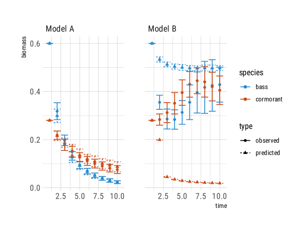
Figure 1: Forecast performance and realized outcomes from management of a 5-species system under either model. Based on forecast performance alone, Model A clearly performs better, accurately predicting steady declines. Model B predicts overly optimistic outcomes for Bass population levels, and overly pessimistic outcomes for cormorants, with observed dynamics falling well outside the predicted range. Despite this, net utility achieved under this management regime is virtually optimal, while the declines under model A result in net utility that is only 38% of optimal.

An Iterative Decision Example

While this example demonstrates that the model which provides the better forecast does not necessarily lead to a better decision, it may raise more questions than it answers. Why does this happen? Is this an isolated example or not? Can this forecast trap be resolved by more sophisticated approaches to model selection and decision-making? I now consider scenarios involving iterative forecasts and adaptive management: in which the manager monitors outcomes, compares forecasts to observations and updates model estimates. Such sequential decision processes are not merely iterative versions of single-decision problems, but are much more challenging. In the opening example, the manager had to choose the harvest policy for each fish species at the start of the scenario and stick with it. The ability to select new actions in response to new observations turns that decision into a game of chess: each turn, the manager must consider not only their next move but all possible series of moves.

How do we translate a model-based forecast into a decision policy? It is impossible to discuss outcomes associated with a forecast without first agreeing on this process. In practice, decision-makers may use a forecast in a wide variety of ways in selecting a course of action, including ways which may run counter to the stated objectives of management (Ludwig et al. 1993). In principle at least, the field of decision theory provides a formal mechanism for determining the optimal strategy given a model forecast. For instance, a wide range of ecological conservation and management problems can be expressed as a Markov Decision Process (MDP) problems (Marescot et al. 2013). Existing computer algorithms such as stochastic dynamic programming (SDP) take a probabilistic model forecast (more precisely, the probability $P(x_{t+1}|x_{t},a_{t})$ of the system being in state $x_{t+1}$ in the next iteration given that it was previously in state $x_{t}$ and the manager selected action $a_{t}$) and the desired management objective (i.e. the maximize the expected biomass of species protected or the expected dollar profit of a fishery (see Clark 1990; Halpern et al. 2013)) as input, and return the decision policy which maximizes that objective (Marescot et al. 2013). This provides a principled way to associate a decision policy with any given forecast model.

Two features of this approach are worth emphasizing. As before, the resulting decision is derived directly from the forecast model and the desired objective. The SDP algorithm is a reasonable description of the approach any ideal manager would use – considering all possible outcomes from all possible sequences of actions and selecting the best sequence. For complex models this process is too laborious even for a computer, and is often simplified by considering only a selection of predetermined policies (as in Management Strategy Evaluation, MSE, Punt et al. (2016)), or scenarios (as in scenario analysis, Polasky et al. (2011)). Such shortcuts are often necessary for complex real-world models, but open additional room for error: the policy we derive from a given forecast may perform poorly not because the model forecast was at fault, but because of those simplifying assumptions about possible policies. To ensure that the forecast trap is not a result of such assumptions about possible policies, we will consider a problem simple enough to solve directly with SDP. The resulting decision policy is optimal, so long as the forecast model is correct. In this way, the SDP merely stands in for a mathematically precise way in which forecasts are turned into decisions. Recognizing the SDP-derived policy (A) comes directly from the forecast model, and (B) gives the optimal policy for said forecast, seems to suggest that whichever model makes the better forecast will surely also lead to better outcomes (as measured in terms of whatever utility we have chosen to maximize). While this intuition is no doubt often accurate, our purpose here is to demonstrate that it is by no means guaranteed: it is also possible for the model which makes the better forecast to lead to worse outcomes.

Let us consider the management of single species in which we seek to maximize the long-term net harvest. In this scenario, the manager estimates the population size each year and must set the total allowable catch (TAC) for that season. The underlying dynamics are unknown, but the manager is presented with any of a variety of forecast models which can predict the future stock sizes given the current population size and proposed TAC. Our manager does not know which of these models is the most accurate a priori. Instead, the manager will be able to compare the population size predicted by each forecast (under the chosen TAC) to the measurement of the population size in the following year before coming up with the next year’s catch limit.

Faced with a collection of models, a manager can seek either to identify the best model to use, or to consider an integrative assessment which uses the whole ensemble of models to represent the manager’s uncertainty about the underlying process. I will consider both approaches in turn. Figure 2 compares forecasts generated by two of the candidate models to observations drawn from simulations of the underlying process. As before, these are true forecasts: the model forecasts are generated first, they have not been fit to these observations. In the un-fished scenario (top panels), both models try to predicting the same un-fished equilibrium dynamics. In the second scenario (lower panel), the manager uses the optimal SDP policy derived from each forecast to determine the TAC for the following year, and compares the observed stock size to that which the model predicted given that fishing quota. In both cases, model 2 provides far more accurate forecasts, as seen in the error bars and confirmed by the distribution of proper scores [Fig 2C-D; Gneiting & Raftery (2007)]. Model and simulation details are provided in Appendix B.

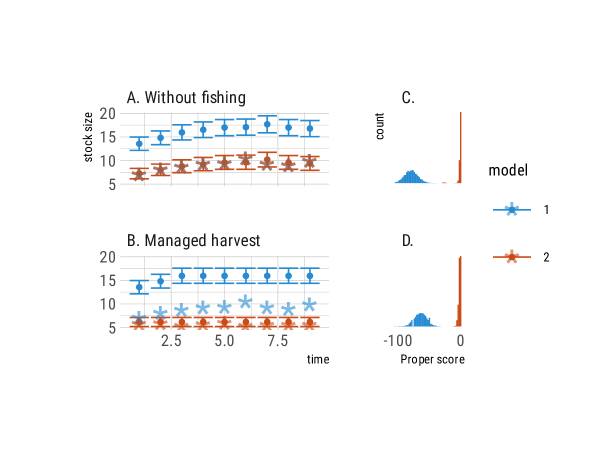
Figure 2: Forecast performance of each model. Panels A, B: Step ahead predictions of stock size under unfished (A) and fished (B) scenarios. Error bars indicating the 95% confidence intervals around each prediction, while stars denote the observed value in that year. Because the models make different decisions each year in the fished scenario, the observed stock size in year 2, 3, etc under the management of model 1 (blue stars) is different from that under model 2 (red stars). Panels C, D: corresponding distribution of proper scores across all predictions (100 replicates of 100 timesteps). Higher scores are better, confirming that model 2 makes the better forecasts.

Despite the clearly superior predictive accuracy of model 2 in both scenarios, the outcomes from management under model 2 are substantially worse. We can assess such outcomes in less abstract terms than forecasting skill, such as economic value them manager sought to optimize (in dollars) or the ecological value (unharvested biomass) [Fig 3].

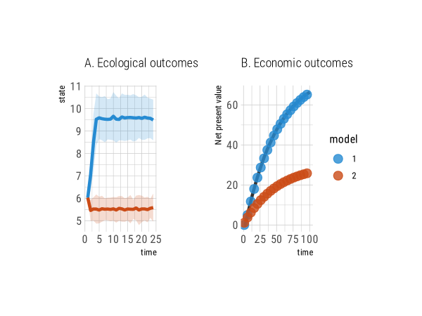
Figure 3: Ecological and economic performance of each forecast. Harvest quotas derived from model 1 result in a significantly higher fish stock size than under Model 2 (panel A). Economic returns under model 1 are also substantially higher (panel B)

A manager operating under model 2 would have little indication that the model was flawed: both future stock sizes and expected harvest yields consistently match model predictions. This manager would be stuck in the forecast trap, incorrectly mistaking a degraded ecological state and reduced economic outcomes as the best that can be achieved because future observations continue to validate this model. Had we been able to include Model 3 in our forecast comparisons, it would equal or outperform the forecasting skill of both model 1 and model 2 (as guaranteed by the theorem of Gneiting & Raftery (2007)), while also matching the economic utility of model 1 (as guaranteed by the theorem of Reed (1979)). In practice, we never have access to the generating model, so it is reasonable to expect model selection to determine the better approximation. As we see here, the better approximation for forecasting future states does not in fact lead to better outcomes.

Adaptive Management

Rather than select a single best model (or best parameter value), a manager could choose to integrate over possible outcomes generated from all candidate models. Updating posterior distributions over parameters and/or weights assigned to different models are examples of this kind of adaptive management (Ludwig & Walters 1982; Punt et al. 2016). I illustrate the application of such an adaptive management strategy, following classic examples for parameter (Ludwig & Walters 1982) or structural (Smith & Walters 1981) model uncertainty. I first consider only the same two models considered in the previous example. I later consider a larger suite of 42 models, spanning the parameter space of Gordon-Schaefer curves. To avoid failure to explore sufficiently, (see exploration-exploitation trade-off, e.g. Walters 1981), I assign prior belief of 99% weight on the optimally performing model, model 1.
For comparison, I consider the baseline case in which the manager does not update posterior distribution over which models/parameter values are correct (the manager still chooses a new TAC after each observation, but does not update their belief in the model, i.e. does not learn over time). The difference between the performance with and without learning is known as the “Value of Information” (Howard 1966). In both 2-model and 42-model scenarios, the value of information is strongly negative. The 2-model case achieves a net present value to -58% of the value of having used model 1 alone [Fig 4]. Including all 42 models reduces this to a value of -32%. Both harvests and fish biomass remain significantly lower under adaptive learning scenarios.

Figure 4: Adaptive management under model uncertainty. Solid lines trace the trajectories of the state (fish stock, circles) and action (harvest quota, triangles), under adaptive management (learning). Dotted lines trace the corresponding trajectories if iterative learning is omitted, leaving the prior belief fixed throughout the simulation (planning). Color indicates the belief that model 1 is correct (blue), with an initial prior belief of 99%. Panel A: Management over the two candidate models, Model 1 and Model 2. Within a single iteration of adaptive management, the belief over models switches from a prior belief that heavily favored model 1 to a posterior that favors model 2 with near certainty. Future iterations reinforce the belief in model 2, resulting in both depressed harvests and low stock sizes (solid lines). If no iterative learning updates are performed, stock sizes and realized harvests (and thus economic profit) are both higher. Panel B: given 42 candidate models over a broad range of parameter values, adaptive management quickly reduces the probability of model 1, and substantially underperforms management without learning (dotted lines). While outcomes improve marginally relative to the two-model case (panel A) they remain significantly worse than had no iterative learning been included.

The reason for model 1’s seemingly contradictory ability to make good decisions but bad forecasts becomes obvious once we compare both curves to that of the underlying model, model 3. Looking at plots of the growth rate curves for each model [Fig 5A], it is hardly surprising that all model selection approaches prefer the closely overlapping curve of model 2 to the no-where-close curve of model 1 as the better approximation of model 3. Nevertheless, the decision policy derived from model 1 forecasts is indistinguishable from that based on the true model [Fig 5B], while the policy derived from model 2 forecasts lead to over-harvesting. Being closest to the true model’s forecast skill never guarantees that we are closest to the true model’s optimal policy.

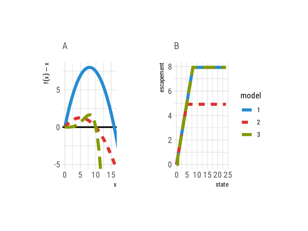
Figure 5: Panel A: Population growth curves of each model. The positive equilibrium of each model occurs where the curve crosses the horizontal axis. Note that while Model 2 is a better approximation to the truth (Model 3), Model 1 better approximates the stock size which leads to maximum growth. Panel B: The optimal control policy under Model 1 is nearly identical to that under the true Model 3, while the optimal policy under Model 2 suppresses stock to a much lower escapement level.

How can the very different forecasts from model 1 and model 3 could produce exactly the same optimal management policy (Fig 5B) under the SDP algorithm? Analytic solutions offer more insight as to when and why very different forecasts can generate the identical policy. Such a solution was first provided by Reed (1979), who demonstrated the optimal policy in the case considered here would be a so-called “bang-bang” policy. Intuitively one can think of this as maintaining the biomass at the most productive size: the maximum population growth rate (position of the peak of the growth curves in Fig 5A), though this is only precisely true without discounting ($\delta=1$): the optimal stock size $\hat{x}$ is the solution to $f(\hat{x})=\hat{x}/\delta$ when stochasticity is sufficiently small (Reed 1979). Thus, all models in which the peak growth rate occurs at the same stock size will have the same optimal policy. These are not merely bad models getting lucky – all such models correctly capture the crucial feature relevant to the decision. In more complex models, such features are more difficult or impossible to identify analytically; but this does not mean they do not exist. For instance, Recent mathematical breakthroughs such as Holden & Conrad (2015), Hening et al. (2019), and Hening (2021) have proven that the optimal harvest control rule in age-structured and predator-prey systems maintain similar bang-bang dynamics. This means that the optimal policy of such very complex models will once again be shared by infinite number of simpler models.

Discussion

The forecast trap illustrated in both examples can best be understood as a problem of non-uniqueness (Oreskes et al. 1994). Even modestly complex models can successfully predict the observed dynamics, but for wrong mechanistic reasons (Schnute & Richards 2001; Schindler & Hilborn 2015). In both examples, a decision-maker who accepts the model which leads to very accurate predictions as the basis for their decision-making winds up in the forecast trap: accepting poor ecological and economic outcomes as the best possible option. The space of possible models is infinitely large when measured against any a scalar metric such as mean forecast skill or expected net utility. Perhaps it should be no surprise then that many models will achieve the same policy outcomes or achieve comparable predictive accuracy. Just as the forecast skill is not unique, both examples also demonstrated that the optimal policy is not unique to the “true model” – many models will result in the same policy and achieve the same outcomes; despite making very different forecasts.

The forecast trap is likely to be more common in contexts in which systems are more complex, partially observed, and available actions are constrained – all features which are particularly common to ecological management and conservation. Because simplicity of the second example allows analytic theory to reveal a precise explanation, it is tempting to assume the trap is only a consequence of examining overly simple models. In fact, the opposite is true. In the second example, the “true” model is simple enough to be covered by a suitable candidate set of models (e.g. a Gaussian Process, Boettiger et al. (2015)), which would resolve the trap given sufficient data. In reality, our models never span the true process. Partially-observed systems increase the space of possible models that achieve comparable predictive accuracy. Constraints on action space such as adjustment costs (Boettiger et al. 2016) or piecewise-linear control rules (Punt 2010) increase the space of models which will result in the same policy. Both of these aspects make the forecast trap easier to encounter in our opening example.

The forecast trap demonstrates that for certain ensembles of candidate models, the value of information (VOI) (Howard 1966; Katz et al. 1987) can in fact be negative. Consequently, methods to select models or re-estimate parameters can lead to worse outcomes than had these new observations simply been ignored. Crucially, a manager implementing the optimal policy from the most predictive model sees no indication that their models are wrong – the declining ecosystem and economic returns observed under model A in the first example or under iterative learning in the second example are completely consistent with and predicted by the models. Only by winding back the clock, making decisions based over the original uncertainty without learning (Fig 4), can we see that better outcomes could have been achieved. The policy derived without learning reflects greater uncertainty: it is thus more robust.

A way forward

In practice, managers rarely rely only on forecasting skill to assess models, nor determine policies directly from forecasts alone. In both examples presented above, the forecast trap is most likely in circumstances where the collection of candidate models is insufficiently broad. Management practice tends to emphasize approaches which broaden rather than narrow down this candidate set. This reflects the view that “the primary values of ecosystem models are as heuristic tools for communication and for developing scenarios to express uncertainties and test policies” rather than as a source of reliable forecasts (Schindler & Hilborn 2015). Such practices include:

1. emphasizing a better articulation of uncertainty a priori;

2. active exploration of alternative policies can reveal when the model set is inadequate

3. methods for generating strategies that are robust to the sort of uncertainty described here.

A central role of models is to help articulate uncertainty around possible outcomes rather than make precise predictions. As Schindler & Hilborn (2015) notes, “current approaches to verification and validation of ecosystem models likely produce overly optimistic impressions of the reliability of forecasts underlying management and conservation prescriptions.” Forecasts based on non-mechanistic models such as empirical dynamical modeling (EDM, Ye et al. 2015; Brias & Munch 2021) may help in articulating a broader ensemble of scenarios (Boettiger et al. 2015). In contrast, if such approaches are selected solely on forecasting skill, they may increase the probability of the forecast trap. The danger of an insufficiently broad model ensemble is well understood in many disciplines which use scenario planning to assist policy in accounting for irreducible uncertainties (Peterson et al. 2003).

Second, a manager may also escape the forecast trap by exploring actions which are never recommended from any of the available forecasts. For example, a manager looking at the low stocks and poor harvests achieved under model 2, could decide experimentally to reduce fishing quota. This will allow the population to enter a range of state-space where discrepancies between model 2 and observations are more obvious. Runge et al. (2016) describes how such “double-loop learning” can be used to identify when the entire model set is inaccurate, a problem which is not solved by “single-loop” adaptive-management in our examples above. Schindler & Hilborn (2015) also underscores the value of flexible policies; rather than “managing solely within the range of past variation; active probing is usually needed,” and contrasts this to a typical interpretation of the ‘precautionary principle’ often cited as a reason to avoid exploratory actions. However, just because active exploration can escape the forecast trap does not mean it is always a good idea.

Third, managers may emphasize policy robustness over forecast skill (Schindler & Hilborn 2015). In many formal treatments, this is not qualitatively different to the analysis considered here: a manager simply chooses a different utility function, such as minimizing ‘regret’ rather than maximizing expected value (Polasky et al. 2011). Such approaches are just as vulnerable to bad outcomes (as defined by their own utility functions) whenever models are selected only on the basis of forecast skill. Alternative approaches may not seek any such optimization, emphasize the viability (Aubin 1991) of possible policy under constraints. In practice, robust design may emphasize acceptable performance across the widest possible array of scenarios (e.g. candidate models). This acts more like a sensitivity analysis of utility with respect to underlying assumptions, rather than an optimization routine (Fischer et al. 2009; e.g. Punt et al. 2016). Computationally, the former is much simpler, allowing researchers to evaluate the performance of a policy on more complex simulations for which calculating the optimal policy would be prohibitively difficult.

Finally, it is worth noting that decisions do not need to be premised on a forecast at all, but can be premised entirely on the basis of past experience: ‘If the fish stock size has gone up, increase harvest slightly, otherwise, decrease slightly.’ Such a policy is not optimal, but it is robust across a wide range of unimodal stock-recruitment curves without ever estimating a predictive model. This is the basis of so-called ‘model-free’ reinforcement learning algorithms such as DQN (Mnih et al. 2015) and SAC (Haarnoja et al. 2018), which train deep neural networks to learn a policy without ever attempting to predict future states of the underlying process. Training such a artificial intelligence agents across a wide suite of simulations, a process known as curriculum learning (Graves et al. 2017), mimics the scenario analyses and search for robust policies. Such approaches have been used to train agents to play 2600 Atari console games at superhuman ability (Mnih et al. 2015), outperform race-car drivers (Wurman et al. 2022) and control nuclear fusion reactions (Degrave et al. 2022). Such approaches are also not yet well understood, introducing new risks as well as new possibilities(Dulac-Arnold et al. 2019; Henderson et al. 2019).

Acknowledgements

The author acknowledges support from NSF CAREER Award #1942280 and helpful discussions with Melissa Chapman. The author is also deeply grateful to the Michael Runge, Chih-hao Hsieh, Antoine Brias, and other anonymous reviewers whose detailed feedback and insights have greatly shaped the paper and my own understanding of these issues.

References

reAubin, J.P. (1991). Viability theory. Systems & control. Birkhauser, Boston.

preBoettiger, C. (2021). Ecological management of stochastic systems with long transients. Theoretical Ecology, 14, 663–671.

preBoettiger, C., Bode, M., Sanchirico, J.N., LaRiviere, J., Hastings, A. & Armsworth, P.R. (2016). Optimal management of a stochastically varying population when policy adjustment is costly. Ecological Applications, 26, 808–817.

preBoettiger, C., Mangel, M. & Munch, S. (2015). Avoiding tipping points in fisheries management through Gaussian process dynamic programming. Proceedings of the Royal Society B: Biological Sciences, 282, 20141631–20141631.

preBrias, A. & Munch, S.B. (2021). Ecosystem based multi-species management using Empirical Dynamic Programming. Ecological Modelling, 441, 109423.

preBurnham, K.P. & Anderson, D.R. (1998). Practical Use of the Information-Theoretic Approach. In: Model Selection and Inference. Springer New York, New York, NY, pp. 75–117.

preChadès, I., McDonald-Madden, E., McCarthy, M.a., Wintle, B., Linkie, M. & Possingham, H.P. (2008). When to stop managing or surveying cryptic threatened species. Proceedings of the National Academy of Sciences, 105, 13936–40.

preClark, C.W. (1973). Profit maximization and the extinction of animal species. Journal of Political Economy, 81, 950–961.

preClark, C.W. (1990). Mathematical Bioeconomics: The Optimal Management of Renewable Resources, 2nd Edition. Wiley-Interscience.

preClark, J.S., Carpenter, S.R., Barber, M., Collins, S., Dobson, A., Foley, J.A., et al. (2001). Ecological Forecasts: An Emerging Imperative. Science, 293, 657–660.

preCostello, C., Ovando, D., Clavelle, T., Strauss, C.K., Hilborn, R., Melnychuk, M.C., et al. (2016). Global fishery prospects under contrasting management regimes. Proceedings of the National Academy of Sciences, 113, 5125–5129.

preDegrave, J., Felici, F., Buchli, J., Neunert, M., Tracey, B., Carpanese, F., et al. (2022). Magnetic control of tokamak plasmas through deep reinforcement learning. Nature, 602, 414–419.

preDietze, M.C., Fox, A., Beck-Johnson, L.M., Betancourt, J.L., Hooten, M.B., Jarnevich, C.S., et al. (2018). Iterative near-term ecological forecasting: Needs, opportunities, and challenges. Proceedings of the National Academy of Sciences, 115, 1424–1432.

preDulac-Arnold, G., Mankowitz, D. & Hester, T. (2019). Challenges of Real-World Reinforcement Learning. arXiv:1904.12901 [cs, stat].

preFischer, J., Peterson, G.D., Gardner, T.A., Gordon, L.J., Fazey, I., Elmqvist, T., et al. (2009). Integrating resilience thinking and optimisation for conservation. Trends in ecology & evolution, 24, 549–54.

preGinzburg, L.R. & Jensen, C.X.J. (2004). Rules of thumb for judging ecological theories. Trends in Ecology & Evolution, 19, 121–126.

preGneiting, T. & Raftery, A.E. (2007). Strictly Proper Scoring Rules, Prediction, and Estimation. Journal of the American Statistical Association, 102, 359–378.

preGraves, A., Bellemare, M.G., Menick, J., Munos, R. & Kavukcuoglu, K. (2017). Automated Curriculum Learning for Neural Networks. arXiv:1704.03003 [cs].

preHaarnoja, T., Zhou, A., Abbeel, P. & Levine, S. (2018). Soft Actor-Critic: Off-Policy Maximum Entropy Deep Reinforcement Learning with a Stochastic Actor. arXiv:1801.01290 [cs, stat].

preHalpern, B.S., Klein, C.J., Brown, C.J., Beger, M., Grantham, H.S., Mangubhai, S., et al. (2013). Achieving the triple bottom line in the face of inherent trade-offs among social equity, economic return, and conservation. Proceedings of the National Academy of Sciences, 110, 6229–34.

preHenderson, P., Islam, R., Bachman, P., Pineau, J., Precup, D. & Meger, D. (2019). Deep Reinforcement Learning that Matters. arXiv:1709.06560 [cs, stat].

preHening, A. (2021). Coexistence, Extinction, and Optimal Harvesting in Discrete-Time Stochastic Population Models. Journal of Nonlinear Science, 31, 1.

preHening, A., Nguyen, D.H., Ungureanu, S.C. & Wong, T.K. (2019). Asymptotic harvesting of populations in random environments. Journal of Mathematical Biology, 78, 293–329.

preHolden, M.H. & Conrad, J.M. (2015). Optimal escapement in stage-structured fisheries with environmental stochasticity. Mathematical Biosciences, 269, 76–85.

preHoward, R. (1966). Information Value Theory. IEEE Transactions on Systems Science and Cybernetics, 2, 22–26.

preKatz, R.W., Brown, B.G. & Murphy, A.H. (1987). Decision-analytic assessment of the economic value of weather forecasts: The fallowing/planting problem. Journal of Forecasting, 6, 77–89.

preLande, R., Engen, S. & Saether, B.-E. (1994). Optimal harvesting, economic discounting and extinction risk in fluctuating populations. Nature, 372, 88–90.

preLi, S.-L., Bjørnstad, O.N., Ferrari, M.J., Mummah, R., Runge, M.C., Fonnesbeck, C.J., et al. (2017). Essential information: Uncertainty and optimal control of Ebola outbreaks. Proceedings of the National Academy of Sciences, 114, 5659–5664.

preLudwig, D., Hilborn, R. & Walters, C. (1993). Uncertainty, Resource Exploitation, and Conservation: Lessons from History. Science, 260, 17–36.

preLudwig, D. & Walters, C.J. (1982). Optimal harvesting with imprecise parameter estimates. Ecological Modelling, 14, 273–292.

preMarescot, L., Chapron, G., Chadès, I., Fackler, P.L., Duchamp, C., Marboutin, E., et al. (2013). Complex decisions made simple: A primer on stochastic dynamic programming. Methods in Ecology and Evolution, 4, 872–884.

preMnih, V., Kavukcuoglu, K., Silver, D., Rusu, A.A., Veness, J., Bellemare, M.G., et al. (2015). Human-level control through deep reinforcement learning. Nature, 518, 529–533.

preNitzbon, J., Heitzig, J. & Parlitz, U. (2017). Sustainability, collapse and oscillations in a simple World-Earth model. Environmental Research Letters, 12, 074020.

preOreskes, N., Shrader-Frechette, K. & Belitz, K. (1994). Verification, Validation, and Confirmation of Numerical Models in the Earth Sciences. Science, 263, 641–646.

prePeterson, G.D., Cumming, G.S. & Carpenter, S.R. (2003). Scenario Planning: A Tool for Conservation in an Uncertain World. Conservation Biology, 17, 358–366.

prePolasky, S., Carpenter, S.R., Folke, C. & Keeler, B. (2011). Decision-making under great uncertainty: environmental management in an era of global change. Trends in Ecology & Evolution, 26, 398–404.

prePunt, A.E. (2010). Harvest control rules and fisheries management. In: Handbook of Marine Fisheries Conservation and Management . (eds. Grafton, RQ, Hilborn, R, Squires, D, Tait, M & Williams, M). Oxford University Press.

prePunt, A.E., Butterworth, D.S., Moor, C.L. de, De Oliveira, J.A.A. & Haddon, M. (2016). Management strategy evaluation: Best practices. Fish and Fisheries, 17, 303–334.

preReed, W.J. (1979). Optimal escapement levels in stochastic and deterministic harvesting models. Journal of Environmental Economics and Management, 6, 350–363.

preRichards, S.A., Possingham, H.P. & Tizard, J. (1999). Optimal Fire Management for Maintaining Community Diversity. Ecological Applications, 9, 880–892.

preRunge, M.C., Stroeve, J.C., Barrett, A.P. & McDonald-Madden, E. (2016). Detecting failure of climate predictions. Nature Climate Change, 6, 861–864.

preSchindler, D.E. & Hilborn, R. (2015). Prediction, precaution, and policy under global change. Science, 347, 953–954.

preSchnute, J.T. & Richards, L.J. (2001). Use and abuse of fishery models. Canadian Journal of Fisheries and Aquatic Sciences, 58, 10–17.

preShea, K., Tildesley, M.J., Runge, M.C., Fonnesbeck, C.J. & Ferrari, M.J. (2014). Adaptive Management and the Value of Information: Learning Via Intervention in Epidemiology. PLoS Biology, 12, 9–12.

preSmith, A.D.M. & Walters, C.J. (1981). Adaptive Management of Stock–Recruitment Systems. Canadian Journal of Fisheries and Aquatic Sciences, 38, 690–703.

preWalters, C.J. (1981). Optimum Escapements in the Face of Alternative Recruitment Hypotheses. Canadian Journal of Fisheries and Aquatic Sciences, 38, 678–689.

preWalters, C.J. & Hilborn, R. (1978). Ecological Optimization and Adaptive Management. Annual Review of Ecology and Systematics, 9, 157–188.

preWilson, K.A., McBride, M.F., Bode, M. & Possingham, H.P. (2006). Prioritizing global conservation efforts. Nature, 440, 337–340.

preWorm, B., Barbier, E.B., Beaumont, N., Duffy, J.E., Folke, C., Halpern, B.S., et al. (2006). Impacts of biodiversity loss on ocean ecosystem services. Science (New York, N.Y.), 314, 787–90.

preWorm, B., Hilborn, R., Baum, J.K., Branch, T.A., Collie, J.S., Costello, C., et al. (2009). Rebuilding global fisheries. Science (New York, N.Y.), 325, 578–85.

preWurman, P.R., Barrett, S., Kawamoto, K., MacGlashan, J., Subramanian, K., Walsh, T.J., et al. (2022). Outracing champion Gran Turismo drivers with deep reinforcement learning. Nature, 602, 223–228.

preYe, H., Beamish, R.J., Glaser, S.M., Grant, S.C.H., Hsieh, C., Richards, L.J., et al. (2015). Equation-free mechanistic ecosystem forecasting using empirical dynamic modeling. Proceedings of the National Academy of Sciences, 112, E1569–E1576.

p