Limiting Distributions of the Likelihood Ratio Test Statistics
for Independence of Normal Random Vectors

Mingyue Hu^a,b,    Yongcheng Qi^a

^aDepartment of Mathematics and Statistics, University of Minnesota Duluth, 1117 University Drive, Duluth, MN 55812, USA

^bSchool of Mathematics and Statistics, Southwest University, 400715 Chongqing, China

Abstract. Consider the likelihood ratio test (LRT) statistics for the independence of sub-vectors from a $p$-variate normal random vector. We are devoted to deriving the limiting distributions of the LRT statistics based on a random sample of size $n$. It is well known that the limit is chi-square distribution when the dimension of the data or the number of the parameters are fixed. In a recent work by Qi, Wang and Zhang (Ann Inst Stat Math (2019) 71: 911–946), it was shown that the LRT statistics are asymptotically normal under condition that the lengths of the normal random sub-vectors are relatively balanced if the dimension $p$ goes to infinity with the sample size $n$. In this paper, we investigate the limiting distributions of the LRT statistic under general conditions. We find out all types of limiting distributions and obtain the necessary and sufficient conditions for the LRT statistic to converge to a normal distribution when $p$ goes to infinity. We also investigate the limiting distribution of the adjusted LRT test statistic proposed in Qi, Wang and Zhang (2019). Moreover, we present simulation results to compare the performance of classical chi-square approximation, normal and non-normal approximation to the LRT statistics, chi-square approximation to the adjusted test statistic, and some other test statistics.

Keywords: Likelihood ratio test; normal random vector; central limit theorem; chi-square approximation; non-normal limit; high dimension; independence

AMS 2020 Subject Classification: 62E20; 62H15

1 Introduction

In classical theory for inference, many statistical methods have been developed to test parametric hypotheses in the last few decades. One of the most popular methods is the so-called likelihood ratio test (LRT). It is known that the distribution functions of LRT statistics can be well approximated by a chi-square distribution under certain regularity conditions when the dimension of the data or the number of the parameters of interest are fixed. This means that one does not have to estimate the variance of the test statistics based on the likelihood ratio.

Many modern data sets such as financial data and modern manufacturing data are high-dimensional. Classical methods may not be adequate for high dimensional data anymore, especially when the dimension of data is relatively large compared with the sample size. Some recent papers have investigated the limiting distribution of the LRT statistics concerning the dependence structures of the multivariate normal distributions. It turns out that the chi-square approximation fails while the dimension of the data increases with the sample size. Instead, the normal approximation to the LRT statistics works well under high dimension setting. See, e.g., Bai et al. [2], Jiang et al. [11], Jiang and Yang [13], Jiang and Qi [12], Qi et al. [17], Dette and Dörnemann [7], and Guo and Qi [9]. Several approaches other than likelihood ratio method have been developed in the literature; See, e.g., Schott [18, 19, 20], Ledoit and Wolf [14], Bao et al. [3], Chen et al. [6], Srivastava and Reid [21], Jiang et al [10], Li et al. [15], and Bodnar et al. [5]. A very recent work by Dörnemann [8] also established the central limit theorems for some LRT statistics under non-normality.

In this paper, we consider a $p$-variate normal random vector and study the limiting distributions of the LRT for testing the independence of its grouped components based on a random sample of size $n$. For a $p$-dimensional multivariate normal distribution with mean vector $\mu$ and covariance matrix $\Sigma$, denoted by $N_{p}(\mu,\Sigma)$, we partition its $p$ components into $k$ subsets and test whether the $k$ sub-vectors are mutually independent, or equivalently, we test whether the covariance matrix $\Sigma$ is block diagonal. In this paper, both $p$ and $k$ can depend on $n$ and diverge with the sample size. On the condition that the lengths of the $k$ sub-vectors are relatively balanced, Qi et al. [17] proved the asymptotic normality and proposed an adjusted test statistic that usually has a chi-square limit when the dimension $p$ goes to infinity with the sample size.

The aim of this paper is to give a complete description for the limiting distributions of the LRT statistic for independence for multivariate normal random vectors. We obtain all possible limiting distributions and give the necessary and sufficient conditions for the central limit theorem. We also investigate the limiting distributions of the adjusted test statistic proposed by Qi et al. [17], which performs better than the normal approximation and chi-square approximation to the LRT statistics in general.

The rest of the paper is organized as follows. In Section 2, we present our main results and establish the necessary and sufficient conditions for the central limit theorem as well as the conditions for non-normal limits. In Section 3, we present some simulation results to compare the performance of four methods including the chi-square approximation to the LRT statistic, the normal and non-normal approximation to the LRT statistic and the chi-square approximation to the adjusted LRT statistic proposed in Qi et al. [17]. In Section 4, we present some preliminary lemmas which are used in Section 5 to prove the main results of the paper.

2 Main results

Let $\chi^{2}_{f}$ denote the random variables following chi-square distribution with $f$ degrees of freedom and $N(0,1)$ the standard normal variables.

For $k\geq 2$, let $q_{1},\cdots,q_{k}$ be $k$ positive integers. Denote $p=q_{1}+q_{2}+...+q_{k}$ and let

$$\Sigma=(\Sigma_{ij})_{1\leq i,j\leq k}$$

be a positive definite matrix, where $\Sigma_{ij}$ is a $q_{i}\times q_{j}$ sub-matrix. Assume $\xi_{i}$ is a $q_{i}$-dimensional normal random vector for each $1\leq i\leq k$, and the $p$-dimensional random vector $(\xi^{\prime}_{1},\cdots,\xi^{\prime}_{k})^{\prime}$ has a multivariate normal distribution $N_{p}(\mu,\Sigma)$. We are interested in testing the independence of $k$ random vectors $\xi_{1},\cdots,\xi_{k}$, or equivalently the following hypotheses

$$H_{0}:\Sigma_{ij}=0~{}\text{for all}~{}~{}1\leq i<j\leq k~{}~{}~{}\text{vs}~{}~{}~{}H_{1}:H_{0}~{}\text{is not true.}$$ (2.1)

Assume that $\mathbf{x}_{1},\cdots,\mathbf{x}_{n}$ are $n$ independent and identically distributed random vectors from distribution $N_{p}(\mu,\Sigma)$. Define

$$\mathbf{A}=\sum_{i=1}^{n}(\mathbf{x}_{i}-\mathbf{\bar{x}})(\mathbf{x}_{i}-\mathbf{\bar{x}})^{\prime},~{}~{}~{}\mathbf{\bar{x}}=\frac{1}{n}\sum_{i=1}^{n}\mathbf{x}_{i},$$

and partition $\mathbf{A}$ as follows

$$\left(\begin{array}[]{cccc}\mathbf{A}_{11}&\mathbf{A}_{12}&\cdots&\mathbf{A}_{1k}\\ \mathbf{A}_{21}&\mathbf{A}_{22}&\cdots&\mathbf{A}_{2k}\\ \vdots&\cdots&\cdots&\vdots\\ \mathbf{A}_{k1}&\mathbf{A}_{k2}&\cdots&\mathbf{A}_{kk}\\ \end{array}\right),$$

where $\mathbf{A}_{ij}$ is a $q_{i}\times q_{j}$ matrix. According to Theorem 11.2.3 from Muirhead [16], the likelihood ratio statistic for testing (2.1) is given by

$$\Lambda_{n}=\frac{|\mathbf{A}|^{\frac{n}{2}}}{\prod_{i=1}^{k}|\mathbf{A}_{ii}|^{\frac{n}{2}}}:=(W_{n})^{\frac{n}{2}}.$$ (2.2)

Note that the likelihood ratio statistic $\Lambda_{n}$ is well defined only if $p<n$. When $p\geq n$, the determinant $|\mathbf{A}|$ is zero since A is singular. Therefore, we can only consider the case $p<n$ in the paper.

We introduce some notations before we give the main results. Let $g$ be any function defined over $(0,\infty)$. For integers $q$ and $n$ with $1\leq q<n$, define

$$\Delta_{g,\,n,\,q}(t)=\sum_{i=1}^{q}g(\frac{n-i}{2}+t),~{}~{}t>-\frac{n-q}{2}.$$ (2.3)

Let $\Gamma(x)$ denote the Gamma function, given by

$$\Gamma(x)=\int^{\infty}_{0}t^{x-1}e^{-t}dt,~{}x>0,$$

and define the digamma function $\psi$

$$\psi(x)=\frac{d\log\Gamma(x)}{dx}=\frac{\Gamma^{\prime}(x)}{\Gamma(x)},~{}x>0.$$ (2.4)

Theorem 2.1.

Assume $p=p_{n}$ satisfy $2\leq p<n$ and $p_{n}\rightarrow\infty$ as $n\rightarrow\infty$. Assume that $q_{1},q_{2},\cdots,q_{k}$ are $k$ positive integers such that $p=\sum_{i=1}^{k}q_{i}$, where $k=k_{n}$ may depend on $n$. Set $q_{\max}=\max\{q_{1},\cdots,q_{k}\}$ and assume $n-q_{\max}\rightarrow\infty$ as $n\rightarrow\infty$. $\Lambda_{n}$ is the Wilks likelihood ratio statistic defined in $\eqref{equ1}$. Then, under the null hypothesis in $\eqref{t1}$

$$T_{0}:=\frac{-2\log\Lambda_{n}-\mu_{n}}{\sigma_{n}}\overset{d}{\longrightarrow}N(0,1)$$ (2.5)

as $n\rightarrow\infty$, where

$$\mu_{n}=-n\big{(}\Delta_{\psi,\,n,\,p}(0)-\sum_{j=1}^{k}\Delta_{\psi,\,n,\,q_{j}}(0)\big{)},$$ (2.6)

$$\sigma_{n}^{2}=2n^{2}\big{(}\sum_{j=1}^{p}\frac{1}{n-j}-\sum_{i=1}^{k}\sum_{j=1}^{q_{j}}\frac{1}{n-j}\big{)}+2n^{2}\big{(}b(n,p)-\sum_{i=1}^{k}b(n,q_{i})\big{)},$$ (2.7)

$$b(n,q)=\sum^{q}_{j=1}\frac{1}{(n-j)^{2}},~{}~{}1\leq q<n,$$ (2.8)

and symbol $\overset{d}{\longrightarrow}$ denotes convergence in distribution.

Now we consider the situation when $n-q_{\max}$ is bounded. In this case, both $n-p$ and $p-q_{\max}$ are bounded because $n-p+p-q_{\max}=n-q_{\max}$. The following theorem gives non-normal limits for $-2\log\Lambda_{n}$ when both $n-p$ and $p-q_{\max}$ are fixed integers.

Theorem 2.2.

Assume $p=p_{n}$ satisfy $2\leq p<n$. Assume $q_{1},q_{2},\cdots,q_{k}$ are $k$ positive integers such that $p=\sum_{i=1}^{k}q_{i}$, where $k=k_{n}$ is an integer that may depend on $n$. Set $q_{\max}=\max\{q_{1},\cdots,q_{k}\}$ and assume $p-q_{\max}=r$ and $n-p=v$ for some fixed integers $r\geq 1$ and $v\geq 1$ for all large $n$. Then, under the null hypothesis in (2.1) we have

$$\frac{-2\log\Lambda_{n}-n\log n}{n}\overset{d}{\longrightarrow}-\sum^{r+v-1}_{j=v}\log Y_{j},$$ (2.9)

where $Y_{j}$, $j\geq 1$ are independent random variables and the $Y_{j}$ has a chi-square distribution with $j$ degrees of freedom.

Remark 1. The classical likelihood method considers the case when both $p$ and $k$ are fixed integers. Assume that $q_{1},q_{2},\cdots,q_{k}$ are fixed for all large $n$, then

$$-2\rho_{n}\log\Lambda_{n}\overset{d}{\longrightarrow}\chi_{f}^{2},$$ (2.10)

where

$$f=\frac{1}{2}\Big{(}p^{2}-\sum_{i=1}^{k}q_{i}^{2}\Big{)},$$ (2.11)

$$\rho_{n}=1-\frac{2\Big{(}p^{3}-\sum_{i=1}^{k}q_{i}^{3}\Big{)}+9\Big{(}p^{2}-\sum_{i=1}^{k}q_{i}^{2}\Big{)}}{6n\Big{(}p^{2}-\sum_{i=1}^{k}q_{i}^{2}\Big{)}};$$ (2.12)

See, e.g., Theorem 11.2.5 in Muirhead [16].

Remark 2. Under conditions that $q_{\max}\leq\delta p$ for some $\delta\in(0,1)$ and $p\to\infty$ as $n\to\infty$, Qi et al. [17] established the following central limit theorem for $-2\log\Lambda_{n}$

$$T_{1}:=\frac{-2\log\Lambda_{n}-\bar{\mu}_{n}}{\tau_{n}}\overset{d}{\longrightarrow}N(0,1)$$

as $n\to\infty$, where

$$\bar{\mu}_{n}=n\sum_{i=1}^{k}(q_{i}-n+\frac{3}{2})\log(1-\frac{q_{i}}{n})-n(p-n+\frac{3}{2})\log(1-\frac{p}{n})+\frac{n}{3}\big{(}b(n,p)-\sum_{i=1}^{k}b(n,q_{i})\big{)},$$ (2.13)

$$\tau_{n}^{2}=2n^{2}\big{(}\sum_{i=1}^{k}\log(1-\frac{q_{i}}{n})-\log(1-\frac{p}{n})\big{)}+2n^{2}\big{(}b(n,p)-\sum_{i=1}^{k}b(n,q_{i})\big{)}.$$

Remark 3. Theorem 2.1 is still true if $\mu_{n}$ is replaced by $\bar{\mu}_{n}$ defined in (2.13) and $\sigma_{n}^{2}$ is replaced by $\bar{\sigma}_{n}^{2}$

$$\bar{\sigma}_{n}^{2}=2n^{2}\big{(}\sum_{j=1}^{p}\frac{1}{n-j}-\sum_{i=1}^{k}\sum_{j=1}^{q_{j}}\frac{1}{n-j}\big{)}.$$ (2.14)

In fact, we have

$$\lim_{n\to\infty}\frac{\mu_{n}-\bar{\mu}_{n}}{\sigma_{n}}=0~{}~{}\mbox{ and}~{}~{}\lim_{n\to\infty}\frac{\bar{\sigma}_{n}^{2}}{\sigma_{n}^{2}}=1$$ (2.15)

if $n-q_{\max}\to\infty$ as $n\to\infty$. The proof of (2.15) is given in Lemma 4.7. In practice, $\mu_{n}$ and $\sigma_{n}^{2}$ should be used since they give better approximation to the mean and variance of $-2\log\Lambda_{n}$, and this selection can achieve a better accuracy for the normal approximation even when $n-q_{\max}$ is not very large.

Remark 4. The distribution of the random variable on the right-hand side of (2.9) is non-normal. This can be verified by using the moment-generating functions. The moment generating function of $\sum^{r+v-1}_{j=v}\log Y_{j}$ is equal to

$$2^{rt}\prod^{r+v-1}_{j=v}\frac{\Gamma(j/2+t)}{\Gamma(j/2)},$$

which cannot be equal to $\exp(\mu t+\sigma^{2}t^{2}/2)$, the moment generating function of a normal random variable with a mean $\mu$ and variance $\sigma^{2}$. Otherwise, after taking the logarithm, it implies that the third derivative of $\sum^{r+v-1}_{j=v}\log\frac{\Gamma(j/2+t)}{\Gamma(j/2)}$ is identically equal to zero. We can show this cannot be true by using some properties of the gamma function. The details are omitted here.

Now we are ready to establish the necessary and sufficient conditions under which the central limit theorem holds for $-2\log\Lambda_{n}$.

Theorem 2.3.

There exist constants $a_{n}\in R$ and $b_{n}>0$ such that under the null hypothesis in (2.1)

$$\frac{-2\log\Lambda_{n}-a_{n}}{b_{n}}\overset{d}{\longrightarrow}N(0,1)$$ (2.16)

if and only if $p_{n}\to\infty$ and $n-q_{\max}\to\infty$ as $n\to\infty$.

From (2.10), (2.5) and (2.9), we have only three different types of limiting distributions for $-2\log\Lambda_{n}$, including chi-square distributions, normal distributions and distributions of linear combinations of logarithmic chi-square random variables. Theoretically, for any $p$ and $q_{i}$’s one can use one of the three limiting distributions to approach the distribution of $-2\log\Lambda_{n}$ when $n$ is large. Since the convergence in (2.10), (2.5) or (2.9) does not provide clear cutoff values for $p$ and $n-q_{\max}$, it may be difficult to select a limiting distribution in practice even if $n$ is very large.

Qi et al. [17] proposed an adjusted log-likelihood ratio test statistic (ALRT) which can be approximated by a chi-square distribution when (2.10) or (2.5) holds. The ALRT is a linear function of $-2\log\Lambda_{n}$ defined as

$$Z_{n}=(-2\log\Lambda_{n})\sqrt{\frac{2f_{n}}{\sigma_{n}^{2}}}+f_{n}-\mu_{n}\sqrt{\frac{2f_{n}}{\sigma_{n}^{2}}}$$ (2.17)

with $f_{n}$, $\mu_{n}$ and $\sigma_{n}^{2}$ being defined in (2.11), (2.6) and (2.7), respectively. We have the following result on chi-square approximation to the distribution of $Z_{n}$.

Theorem 2.4.

Let $p=p_{n}$ be a sequence of integers with $2\leq p<n$. Assume $k=k_{n}$ is also a sequence of positive integers, and $q_{1},\cdots,q_{k}$ are $k$ positive integers such that $p=\sum_{i=1}^{k}q_{i}$. Assume $n-q_{\max}\to\infty$ as $n\to\infty$. Then, under the null hypothesis in (2.1), we have

$$\lim_{n\to\infty}\sup_{-\infty<x<\infty}|P(Z_{n}\leq x)-P(\chi^{2}_{f_{n}}\leq x)|=0.$$ (2.18)

We note that the chi-square approximation in (2.18) does not impose any restriction on dimension $p$ and the number of degrees of freedom of the chi-square distribution changes with $n$.

3 Simulation study

3.1 Comparison of LRT related tests

In this subsection, we carry out a finite-sample simulation study to compare the performance of three different approaches to the likelihood ratio test statistic $-2\log\Lambda_{n}$ under condition $n-q_{\max}\to\infty$ under the null hypothesis in (2.1), including the classical chi-square approximation (2.10), the normal approximation (2.5), and the adjusted chi-square approximation in (2.18). The three approaches are denoted by “Chisq”, “CLT” and “ALRT”, respectively. We will also compare the performance of the normal approximation (2.5), the adjusted chi-square approximation in (2.18) and the non-normal approximation given in (2.9) (denoted by “LogChi”), and the comparison is made under conditions that both $r=p-q_{\max}$ and $v=n-p$ are fixed integers.

For all four approaches, we will demonstrate how well the proposed limiting distributions fit the histograms of the four test statistics. From $\eqref{MGF}$ in Lemma 4.1, the moment-generating function of $\log W_{n}$ is distribution-free under the null hypothesis in $\eqref{t1}$. Since the four test statistics are functions of $\Lambda_{n}$ and hence they are also functions of $\log W_{n}$ from $\eqref{equ1}$, they are distribution-free as well under the null hypothesis in $\eqref{t1}$. Therefore, the underlying distribution in our study is set to be a multivariate normal distribution with independent standard normal components.

In our simulation study, we choose sample size $n=101$. For each of selected combinations of $p$ and $q_{i}$’s under the regimes of the chi-square and normal limiting distributions, we repeat the sampling for $10,000$ times and obtain 10,000 replicates for the four test statistics given in (2.10), (2.5), (2.17), and (2.9). We plot the histogram for each test statistic and its corresponding theoretical density function in one graph.

In the simulation study we consider the following four cases.

Case a. We set $k=3$, $p=10,30,60$ and $90$ and use the ratio $q_{1}:q_{2}:q_{3}=3:1:1$. Figure 1 contains 12 plots in an array with four rows and three columns, and each row corresponds to one value of $p=10,30,60$, and $90$.

Case b. We set $k=2$, $q_{1}=p-1$ and $q_{2}=1$ for $p=10,30,60$, and $90$, respectively. Figure 2 contains 12 plots in an array with four rows and three columns, and each row corresponds to one value of $p=10,30,60$, and $90$.

Case c. We set $k=2$, $p=100$ and choose $(q_{1},q_{2})=(50,50)$, $(60,40)$, $(80,20)$, and $(90,10)$, respectively. Figure 3 contains 12 plots in an array with four rows and three columns, and each row corresponds to one combination of $(q_{1},q_{2})$ with $q_{\max}=50,60,80$, and $90$, respectively.

Case d. We set $n=101$, $k=2$, $r=p-q_{\max}=1$ and and $v=n-p=1$, $3$, $5$ and $10$.

For the first three cases above, we select parameters to maintain a reasonably large value for $n-q_{\max}$ so that we compare the performance of classical chi-square approximation (2.10), the normal approximation (2.5), and the adjusted chi-square approximation in (2.18). Under Case a, the values of $q_{i}$’s are proportional. Under Cases b and c, two extreme situations, either $q_{\max}=p-1$ or $p=n-1$, are considered.

Case d is used to compare the performance of the normal approximation (2.5), the adjusted chi-square approximation in (2.18) and the non-normal approximation in (2.9). Since we take $r=1$, the limit on the right-hand side of (2.9) has only one term, that is, the limit is $-\log Y_{v}$, where $Y_{v}$ is a random variable having a chi-square distribution with $v$ degrees of freedom.

The results under Cases a to d are given in Figures 1 to 4, respectively.

Now we summarize our findings from Figures 1 to 4.

1. The classical chi-square approximation (Chisq) works very well for small $p$, but it becomes worse with the increase of $p$ and finally departs from the histograms of the test statistic.

2. When $p$ is small such as $p=10$, the normal approximation (CLT) shows lack of fit to the histograms and it is getting better with the increase of $p$.

3. The adjusted likelihood ratio method (ALRT) works very well for all cases, that is, for small $p$, the ALRT behaves like the classical chi-square approximation, while for large $p$, it performs very well too like the normal approximation.

4. In Figure 3, we select $p=n-1$. Both the normal approximation and the adjusted likelihood method show a little bit departure from the histograms since $p$ is too close to $n$ and sample size $n=101$ is not a large sample size. In this case, both the normal approximation and the adjusted likelihood method can improve when $n$ is getting larger.

5. From Figure 4, when $v$ is small, the non-normal approximation works much better than the normal approximation and the adjusted chi-square approximation. When the value of $v$ increases from $5$ to $10$, both the normal approximation and the adjusted chi-square approximation improve significantly. This implies that one can use the normal approximation or the adjusted chi-square approximation when $r+v=n-p_{\max}$ is not too small. We note that the exact distribution of the limit on the right-hand side of (2.9) is not easy to obtain if $r=p-q_{\max}>1$.

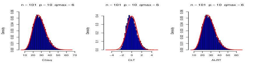
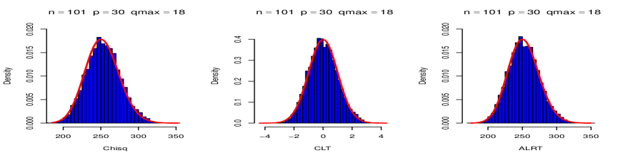
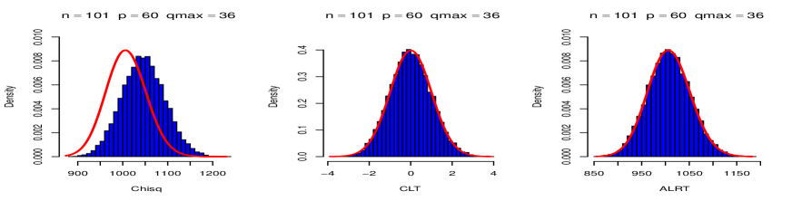
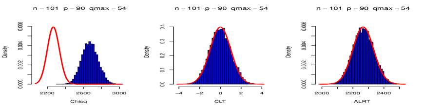
Figure 1: Plots of histograms and theoretical density curves (smooth curves in graphs) for three test statistics based on the classical chi-square approximation (2.10), the normal approximation (2.5), and the adjusted chi-square approximation in (2.18) with selection of $k=3$ and ratio $q_{1}:q_{2}:q_{3}=3:1:1$.

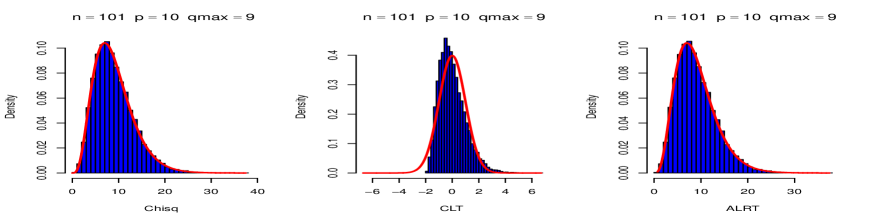
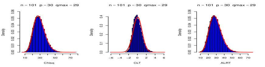
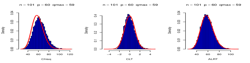
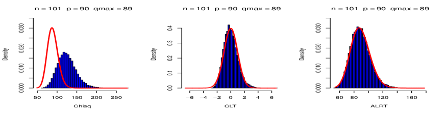
Figure 2: Plots of histograms and theoretical density curves (smooth curves in graphs) for three test statistics based on the classical chi-square approximation (2.10), the normal approximation (2.5), and the adjusted chi-square approximation in (2.18) with selection of $k=2$, $(q_{1},q_{2})=(p-1,1)$ and $p=10,30,60$ and $90$.

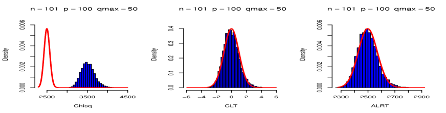
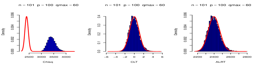
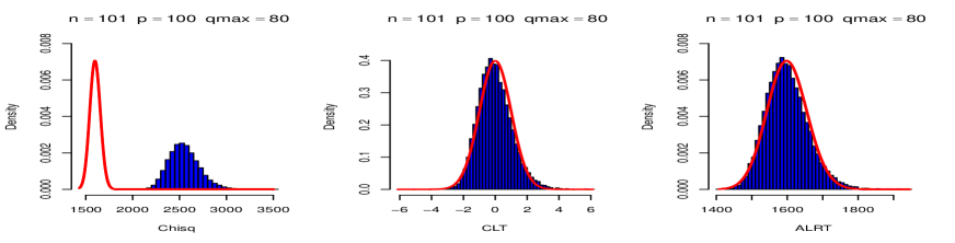
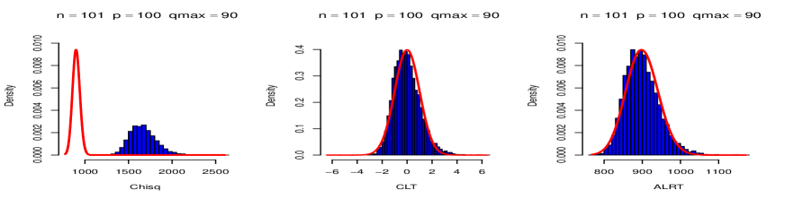
Figure 3: Plots of histograms and theoretical density curves (smooth curves in graphs) for three test statistics based on the classical chi-square approximation (2.10), the normal approximation (2.5), and the adjusted chi-square approximation in (2.18) with selection of $k=2$, $p=100$ and $(q_{1},q_{2})=(50,50)$, $(60,40)$, $(80,20)$, and $(90,10)$.

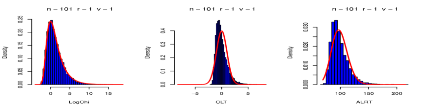
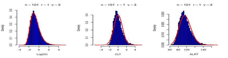
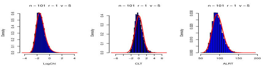
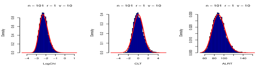
Figure 4: Plots of histograms and theoretical density curves (smooth curves in graphs) for three test statistics based on non-normal approximation (2.9), the normal approximation (2.5), and the adjusted chi-square approximation in (2.18) with selection of $n=101$, $k=2$, $r=p-q_{\max}=1$, and $v=n-p=1,3,5$ and $10$. For the plots in the first column above, LogChi denotes the non-normal approximation in (2.9).

3.2 Comparison of adjusted log-LRT and other methods

In this subsection, we compare our adjusted log-likelihood ratio test statistic, i.e., $Z_{n}$ in (2.17) with other three test statistics, including two trace criterion test statistics by Jiang et al. [10] and Li et al. [15] and Schott type statistics by Bao et al. [3]. We notice that Jiang et al. [10] and Bao et al. [3] investigate their test statistics for test (2.1) for any fixed $k\geq 2$ while Li et al. [15] consider test (2.1) for $k=2$ only. Given that Li et al. [15]’s test statistics are suitable for $k=2$ only, we set $k=2$ for the comparison in this section.

In Jiang et al. [10], a large-dimensional trace criterion test statistic is defined as

$$L_{n}=\textbf{tr}(A_{21}A_{11}^{-1}A_{12}A_{22}^{-1}),$$

where $\textbf{tr}(A)$ denotes the trace of matrix $A$. Under conditions $r_{n1}:=q_{2}/q_{1}\to r_{1}\in(0,\infty)$, $r_{n2}:=q_{2}/(n-1-q_{2})\to r_{2}\in(0,\infty)$, and $q_{2}<n$, it is shown that

$$T_{2}:=\frac{L_{n}-a_{n}}{\sqrt{b_{n}}}\overset{d}{\to}N(0,1)\mbox{ as }n\to\infty$$ (3.1)

under the null hypothesis in (2.1), where

$$b_{n}=\frac{2h_{n}^{2}r_{n1}^{2}r_{n2}^{2}}{(r_{n1}+r_{n2})^{2}},~{}a_{n}=\frac{q_{2}r_{n2}}{r_{n1}+r_{n2}},~{}h_{n}=\sqrt{r_{n1}+r_{n2}-r_{n1}r_{n2}}.$$

Some calculation shows that $a_{n}=q_{1}q_{2}/(n-1)$ and $b_{n}=2q_{1}q_{2}(n-1-q_{1})(n-1-q_{2})/(n-1)^{4}$.

When $k=2$, the test statistic in Bao et al. [3] is equal to

$$\textbf{tr}(A_{22}^{-1/2}A_{21}A_{11}^{-1}A_{12}A_{22}^{-1/2})=\textbf{tr}(A_{21}A_{11}^{-1}A_{12}A_{22}^{-1}),$$

which is the same $L_{n}$. Meanwhile, Theorem 3.1 in [3] also implies (3.1).

To introduce Li et al. [15]’s test statistic, set for $i,j=1,2$

$$\gamma_{ij}=\frac{1}{(n-2)(n+1)}\Big{(}\textbf{tr}(A_{ij}A_{ji})-\frac{1}{n-1}\textbf{tr}(A_{ii})\textbf{tr}(A_{jj})\Big{)}.$$

The trace criterion test statistic by [15] is defined as $\gamma_{12}$. Under the null hypothesis in (2.1) for $k=2$, it is shown in Li et al. [15] that

$$T_{3}:=\sqrt{\frac{(n-2)(n+1)}{2}}\frac{\gamma_{12}}{\sqrt{\gamma_{11}\gamma_{22}}}\overset{d}{\to}N(0,1)\mbox{ as }n\to\infty$$ (3.2)

given that $p=q_{1}+q_{2}\to\infty$ as $n\to\infty$ and

$$0<\lim_{n\to\infty}\frac{1}{p}\textbf{tr}(\mathbf{\Sigma^{i}})<\infty~{}\mbox{ for }i=1,2,4.$$

We notice that the test statistic $T_{3}$ works only for the case $k=2$, but condition $p=q_{1}+q_{2}\to\infty$ is less restrictive than those required for other statistics we just discussed.

For any fixed size $\alpha\in(0,1)$, test $T_{2}$ (or $T_{3}$) rejects the null hypothesis in (2.1) if $T_{2}>z_{\alpha}$ (or $T_{3}>z_{\alpha}$), where $z_{\alpha}$ denotes the $\alpha$-level critical value of the standard normal distribution.

To compare our adjusted log-likelihood ratio test statistic $Z_{n}$ and test statistics $T_{2}$ and $T_{3}$, we assume $q_{1}>q_{2}\geq 1$ and $p=q_{1}+q_{2}<n$. Our samples are generated from the populations similar to those in Jiang et al. [10] and Qi et al. [17]. Let $\mathbf{z}=(z_{1},\cdots,z_{p})^{\prime}$ be a random vector whose components are independent normal random variables with mean $0$ and variance $1$.

Model 1. $\mathbf{x}=(x_{1},\cdots,x_{p})^{\prime}$, where $x_{i}=(1+c)z_{i}$ for $i=1,\cdots,p_{1}$, $x_{p_{1}+j}=z_{p_{1}+j}+cz_{j}$ for $j=1,\cdots,p_{2}$, and $c$ is a constant;

Model 2. $\mathbf{x}=(x_{1},\cdots,x_{p})^{\prime}$, where $x_{i}=(1+c)z_{i}$ for $i=1,\cdots,p_{1}$, $x_{p_{1}+j}=z_{p_{1}+j}+cz_{j}$ for $j=1,\cdots,p_{2}-1$, $x_{p}=p^{-1/4}z_{p}$, and $c$ is a constant.

With different selections of $(q_{1},q_{2},n,c)$, we draw $10000$ random samples of size $n$ from each model above (Model 1 and Model 2) and then we calculate the empirical sizes of the tests (when $c=0$) or the powers of the tests (when $c\neq 0$). The nominal level of size $\alpha$ (type I error) is set to be $0.05$ in the simulation.

Tables 1 and 2 present results for the numerical comparisons on the three test statistics. From the two tables, the adjusted log-likelihood ratio test statistic $Z_{n}$ is constantly accurate in terms of type I error, and $T_{3}$ has larger type I errors than the nominal level $0.05$ for small values of $p$. In view of empirical powers, $Z_{n}$ and $T_{2}$ are comparable in most cases while $T_{3}$ is better than both $Z_{n}$ and $T_{2}$ under Model 1. Under Model 2, $Z_{n}$ has a slightly larger power than $T_{2}$ in most cases and both are significantly better than $T_{3}$.

Table 1: Comparisons on Size and Power under Model 1. The sizes and powers are estimated based on $10,000$ simulations under Model 1, and the nominal type I errors for all tests are set to be $0.05$.

		Size ($c=0$)			Power ($c=0.1$)			Power ($c=0.2$)
($q_{1},q_{2}$)	$n$	$Z_{n}$	$T_{2}$	$T_{3}$	$Z_{n}$	$T_{2}$	$T_{3}$	$Z_{n}$	$T_{2}$	$T_{3}$
(6, 4)	20	0.0507	0.0514	0.0645	0.0605	0.0583	0.0806	0.0909	0.0923	0.1394
	50	0.0507	0.0593	0.0641	0.0857	0.0999	0.1128	0.2400	0.2654	0.3044
	100	0.0527	0.0615	0.0645	0.1350	0.1570	0.1690	0.5643	0.6028	0.6262
(8, 2)	20	0.0498	0.0501	0.0609	0.0532	0.0547	0.0705	0.0717	0.0704	0.1029
	50	0.0487	0.0581	0.0641	0.0699	0.0838	0.0927	0.1499	0.1719	0.1983
	100	0.0530	0.0665	0.0646	0.0957	0.1154	0.1251	0.3086	0.3461	0.3709
(18, 12)	50	0.0499	0.0542	0.0545	0.1897	0.1983	0.2255	0.8617	0.8732	0.9147
	100	0.0506	0.0528	0.0554	0.1233	0.1289	0.1482	0.5492	0.5702	0.6757
	150	0.0499	0.0542	0.0545	0.1897	0.1983	0.2255	0.8617	0.8732	0.9147
(24, 6)	50	0.0499	0.0472	0.0562	0.0647	0.0614	0.0777	0.1133	0.1115	0.1811
	100	0.0478	0.0519	0.0540	0.0854	0.0881	0.1096	0.2990	0.3128	0.3855
	150	0.0547	0.0595	0.0588	0.1214	0.1334	0.1482	0.5393	0.5587	0.6210
(36, 24)	100	0.0511	0.0543	0.0519	0.1053	0.1112	0.1495	0.4243	0.4599	0.6915
	150	0.0493	0.0494	0.0527	0.1619	0.1629	0.2224	0.8144	0.8361	0.9328
	200	0.0538	0.0554	0.0562	0.2428	0.2498	0.3138	0.9715	0.9756	0.9915
(48, 12)	100	0.0519	0.0523	0.0509	0.0771	0.0795	0.1039	0.2235	0.2325	0.3836
	150	0.0503	0.0496	0.0568	0.1115	0.1137	0.1368	0.4657	0.4793	0.6399
	200	0.0473	0.0503	0.0513	0.1471	0.1493	0.1817	0.7222	0.7334	0.8261
(60, 40)	150	0.0499	0.0495	0.0502	0.1248	0.1362	0.2202	0.6453	0.7046	0.9407
	200	0.0524	0.0552	0.0555	0.2036	0.2140	0.3101	0.9358	0.9497	0.9940
	300	0.0532	0.0547	0.0526	0.4046	0.4153	0.5247	1.0000	1.0000	1.0000
(80, 20)	150	0.0501	0.0514	0.0553	0.0907	0.0959	0.1343	0.3269	0.3543	0.6420
	200	0.0521	0.0529	0.0527	0.1287	0.1325	0.1795	0.6093	0.6287	0.8362
	300	0.0507	0.0519	0.0502	0.2162	0.2203	0.2791	0.9453	0.9500	0.9844

Table 2: Comparisons on Size and Power under Model 2. The sizes and powers are estimated based on $10,000$ simulations under Model 2, and the nominal type I errors for all tests are set to be $0.05$.

		Size ($c=0$)			Power ($c=0.1$)			Power ($c=0.2$)
($q_{1},q_{2}$)	$n$	$Z_{n}$	$T_{2}$	$T_{3}$	$Z_{n}$	$T_{2}$	$T_{3}$	$Z_{n}$	$T_{2}$	$T_{3}$
(6, 4)	20	0.0507	0.0514	0.0658	0.0797	0.0798	0.0834	0.1965	0.1991	0.1525
	50	0.0507	0.0593	0.0658	0.1916	0.2083	0.1175	0.7428	0.7472	0.3532
	100	0.0527	0.0615	0.0647	0.4467	0.4774	0.1880	0.9938	0.9945	0.7142
(8, 2)	20	0.0498	0.0501	0.0626	0.0787	0.0763	0.0749	0.1855	0.1805	0.1214
	50	0.0487	0.0581	0.0695	0.1966	0.2178	0.1057	0.7311	0.7443	0.2567
	100	0.0530	0.0665	0.0654	0.4261	0.4626	0.1456	0.9901	0.9921	0.5237
(18, 12)	50	0.0494	0.0492	0.0579	0.1365	0.1330	0.1000	0.5468	0.4722	0.3095
	100	0.0506	0.0528	0.0564	0.4118	0.3876	0.1582	0.9961	0.9841	0.7051
	150	0.0499	0.0542	0.0571	0.7148	0.6869	0.2317	1.0000	1.0000	0.9343
(24, 6)	50	0.0499	0.0472	0.0570	0.1378	0.1279	0.0852	0.5213	0.4103	0.1983
	100	0.0478	0.0519	0.0536	0.4234	0.3949	0.1132	0.9937	0.9718	0.4257
	150	0.0547	0.0595	0.0601	0.7320	0.6968	0.1587	1.0000	1.0000	0.6789
(36, 24)	100	0.0511	0.0543	0.0517	0.2865	0.2672	0.1492	0.9389	0.8449	0.7075
	150	0.0493	0.0494	0.0535	0.6008	0.5303	0.2269	0.9999	0.9979	0.9392
	200	0.0538	0.0554	0.0576	0.8552	0.7843	0.3194	1.0000	1.0000	0.9926
(48, 12)	100	0.0519	0.0523	0.0511	0.2822	0.2407	0.1048	0.9086	0.7314	0.4058
	150	0.0503	0.0496	0.0553	0.6079	0.5098	0.1447	0.9998	0.9906	0.6671
	200	0.0473	0.0503	0.0519	0.8579	0.7741	0.1913	1.0000	0.9999	0.8484
(60, 40)	150	0.0499	0.0495	0.0493	0.3966	0.3446	0.2209	0.9915	0.9530	0.9460
	200	0.0524	0.0552	0.0560	0.7092	0.5988	0.3147	1.0000	0.9993	0.9962
	300	0.0532	0.0547	0.0535	0.9768	0.9346	0.5361	1.0000	1.0000	1.0000
(80, 20)	150	0.0501	0.0514	0.0564	0.3863	0.3046	0.1403	0.9766	0.8280	0.6582
	200	0.0521	0.0529	0.0528	0.7005	0.5473	0.1865	1.0000	0.9924	0.8517
	300	0.0507	0.0519	0.0510	0.9791	0.9093	0.2885	1.0000	1.0000	0.9886

4 Some lemmas

The multivariate gamma function, denoted by $\Gamma_{p}(x)$, is defined as

$$\Gamma_{p}(x):=\pi^{p(p-1)/4}\prod_{i=1}^{p}\Gamma(x-\frac{1}{2}(i-1))$$ (4.1)

with $x>\frac{p-1}{2}$ from Muirhead [16].

For any positive integers $n$ and $p$ with $1<p<n$, let $q_{1},\cdots,q_{k}$ be $k$ positive integers such that $p=\sum^{k}_{i=1}q_{i}$, where $k\geq 2$ is an integer which may depend on $n$. Denote $q_{\max}=\max_{1\leq i\leq k}q_{i}$.

For any function $g$ defined over $(0,\infty)$, set

$$\Psi_{g,\,n,\,p}(x)=\Delta_{g,\,n,\,p}(x)-\sum^{k}_{i=1}\Delta_{g,\,n,\,q_{i}}(x)=\sum^{p}_{j=1}g(\frac{n-j}{2}+x)-\sum^{k}_{i=1}\sum^{q_{i}}_{j=1}g(\frac{n-j}{2}+x)$$ (4.2)

for $x>-\frac{n-p}{2}$, where $\Delta_{g,\,n,\,q_{i}}$ is defined in (2.3). For brevity, we omit $q_{1},\cdots,q_{k}$ in the definition of $\Psi_{g,\,n,\,p}(x)$.

Let $g$ be a differentiable function. Both $\Delta_{g,\,n,\,q}$ and $\Psi_{g,\,n,\,p}$ are linear functionals in $g$ with following property

$$\frac{d}{dx}\Delta_{g,\,n,\,q}(x)=\Delta_{g^{\prime},\,n,\,q}(x),~{}~{}~{}\frac{d}{dx}\Psi_{g,\,n,\,q}(x)=\Psi_{g^{\prime},\,n,\,q}(x).$$ (4.3)

Now we set $\beta_{nr}(x)=\Psi_{g,\,n,\,p}(x)$ when $g(x)=1/x^{r}$ for $r\geq 1$, that is, we define

$$\beta_{nr}(x)=\sum^{p}_{j=1}\frac{1}{\big{(}\frac{n-j}{2}+x\big{)}^{r}}-\sum^{k}_{i=1}\sum^{q_{i}}_{j=1}\frac{1}{\big{(}\frac{n-j}{2}+x\big{)}^{r}},~{}~{}x>-\frac{n-p}{2}.$$ (4.4)

Note that $\beta_{nr}(x)\geq 0$ since $g(x)=1/x^{r}$, $x>0$ is a decreasing function over $(0,\infty)$.

Define

$$s(x)=(x-\frac{1}{2})\log(x)-x,~{}x>0$$

and set

$$h(x)=\log\Gamma(x)-s(x),~{}~{}~{}x>0.$$ (4.5)

Then we can verify that

$$s^{\prime}(x)=\log x-\frac{1}{2x},~{}s^{\prime\prime}(x)=\frac{1}{x}+\frac{1}{2x^{2}},~{}s^{\prime\prime\prime}(x)=-\frac{1}{x^{2}}-\frac{1}{x^{3}},$$ (4.6)

and for some constant $C>0$

$$|h^{\prime\prime}(x)|\leq\frac{C}{x^{3}},~{}~{}~{}x\geq\frac{1}{4};$$ (4.7)

See Lemma 4.4 in Guo and Qi [9].

For the digamma function $\psi$ defined in (2.4), it follows from Formula 6.3.18 in Abramowitz and Stegun [1] that

$$\psi(x)=\log x-\frac{1}{2x}-\frac{1}{12x^{2}}+O(\frac{1}{x^{4}})$$ (4.8)

as $x\rightarrow\infty$.

From now on, we adopt the following notation in our lemmas and our proofs. For any two sequences, $\{a_{n}\}$ and $\{b_{n}\}$ with $b_{n}>0$, notation $a_{n}=o(b_{n})$ implies $\lim_{n\to\infty}a_{n}/b_{n}=0$, and notation $a_{n}=O(b_{n})$ means $a_{n}/b_{n}$ is uniformly bounded.

We first introduce the formula for the $h$-th moment of $W_{n}$.

Lemma 4.1.

(Theorem 11.2.3 in Muirhead [16]) Let $p=\sum_{i=1}^{k}q_{k}$ and $W_{n}$ be Wilk’s likelihood ratio statistics defined in (2.2). Then, under the null hypothesis in (2.1), we have

$$\mathbf{E}(W_{n}^{h})=\frac{\Gamma_{p}(\frac{n-1}{2}+h)}{\Gamma_{p}(\frac{n-1}{2})}\prod_{i=1}^{k}\frac{\Gamma_{q_{i}}(\frac{n-1}{2})}{\Gamma_{q_{i}}(\frac{n-1}{2}+h)}$$ (4.9)

for any $h>\frac{p-n}{2}$, where $\Gamma_{p}(x)$ is defined in (4.1).

Next, we introduce a distributional representation for $W_{n}$.

Lemma 4.2.

(Theorem 11.2.4 in Muirhead [16]) Let $p=\sum_{i=1}^{k}q_{k}$ and $W_{n}$ be Wilk’s likelihood ratio statistics defined in (2.2). Then, under the null hypothesis in (2.1), $W_{n}$ has the same distribution as

$$\prod_{i=2}^{k}\prod^{q_{i}}_{j=1}V_{ij},$$

where $q_{i}^{*}=\sum^{i-1}_{j=1}q_{j}$ for $2\leq i\leq k$, the $V_{ij}$’s are independent random variables and $V_{ij}$ has a beta($\frac{1}{2}(n-q_{i}^{*}-j)$, $\frac{1}{2}q_{i}^{*}$) distribution.

Lemma 4.3.

(Lemma 5 in Qi et al.  [17]) As $n\to\infty$,

$$\sum^{q}_{i=1}(\frac{1}{n-i}-\frac{1}{n-1})=-\frac{q}{n}-\log(1-\frac{q}{n})+O(\frac{q}{n(n-q)}),$$ (4.10)

$$\sum^{q}_{i=1}\Big{(}\log(n-i)-\log(n-1)\Big{)}=(q-n+\frac{1}{2})\log(1-\frac{q}{n})-\frac{(n-1)q}{n}+O(\frac{q}{n(n-q)})$$ (4.11)

uniformly over $1\leq q<n$.

Lemma 4.4.

With $\beta_{nr}$ defined in (4.4), we have

$$\frac{2p}{3n}\log\big{(}1+\frac{p-q_{\max}}{3(n-p)}\big{)}\leq\beta_{n1}(0)\leq\frac{4p}{n}\log\big{(}1+\frac{2(p-q_{\max})}{n-p}\big{)}.$$ (4.12)

$$\beta_{n2}(x)\leq\frac{32\beta_{n1}(0)}{n-p},$$ (4.13)

$$\beta_{n2}(x)\leq\frac{8192p(p-q_{\max})}{n(n-p)(n-q_{\max})}$$ (4.14)

and

$$\beta_{n3}(x)\leq\frac{192\beta_{n1}(0)}{(n-p)^{2}}$$ (4.15)

for all $|x|\leq\frac{n-p}{4}$.

Proof. Without loss of generality, assume $q_{1}\geq q_{2}\geq\cdots\geq q_{k}$. Therefore, $q_{1}=q_{\max}=\max_{1\leq i\leq k}q_{i}$. Set $q_{i}^{*}=\sum^{i-1}_{j=1}q_{j}$ for $2\leq i\leq k+1$. Then we see that

$$\beta_{n1}(0) = 2\sum_{j=1}^{p}\frac{1}{n-j}-\sum_{i=1}^{k}\sum_{j=1}^{q_{i}}\frac{1}{n-j}$$ (4.16)

$$= 2\sum_{i=2}^{k}\sum^{q_{i}}_{j=1}\big{(}\frac{1}{n-q_{i}^{*}-j}-\frac{1}{n-j}\big{)}$$

$$= 2\sum_{i=2}^{k}\sum^{q_{i}}_{j=1}\frac{q_{i}^{*}}{(n-q_{i}^{*}-j)(n-j)}.$$

Note that $q_{i}^{*}\geq q_{1}=q_{\max}$, and $q_{i}^{*}+q_{i}\leq p$ for all $2\leq i\leq k$. Moreover, $q_{i}\leq p/2\leq n/2$ for all $2\leq i\leq k$, and thus $n>n-j\geq n/2$ for $1\leq j\leq q_{i}$, $2\leq i\leq k$. We have

$$\beta_{n1}(0) \leq \frac{4p}{n}\sum_{i=2}^{k}\sum^{q_{i}}_{j=1}\frac{1}{n-q_{i}^{*}-j}$$

$$= \frac{4p}{n}\sum_{j=1}^{p-q_{\max}}\frac{1}{n-q_{\max}-j}$$

$$\leq \frac{4p}{n}\int_{0.5}^{p-q_{\max}+0.5}\frac{1}{n-q_{\max}-x}dx$$

$$= \frac{4p}{n}\log\big{(}\frac{n-q_{\max}-0.5}{n-p-0.5}\big{)}$$

$$= \frac{4p}{n}\log\big{(}1+\frac{2(p-q_{\max})}{n-p}\big{)},$$

which gives the upper bound in (4.12).

To verify the lower bound in (4.12), define $m=\min\{i\geq 2:q_{i}^{*}\geq p/3\}$. We see that $m=2$ if $q_{1}=q_{\max}\geq p/3$. If $q_{1}<p/3$, then $q_{k}\leq\cdots\leq q_{2}\leq q_{1}<p/3$, which implies that $k\geq 4$, $2<m\leq k$, $q_{m-1}^{*}<p/3$, $p/3\leq q_{m}^{*}<2p/3$, and thus, $p-q_{m}^{*}\geq p/3\geq(p-q_{\max})/3$. When $q_{1}<p/3$, it is trivial that $p-q_{m}^{*}\geq p/3\geq(p-q_{\max})/3$. Then we conclude from (4.16) that

$$\beta_{n1}(0) \geq 2\sum_{i=m}^{k}\sum^{q_{i}}_{j=1}\frac{q_{i}^{*}}{(n-q_{i}^{*}-j)(n-j)}$$

$$\geq \frac{2p}{3n}\sum_{i=m}^{k}\sum^{q_{i}}_{j=1}\frac{1}{n-q_{i}^{*}-j}$$

$$= \frac{2p}{3n}\sum_{j=1}^{p-q_{m}^{*}}\frac{1}{n-q_{m}^{*}-j}$$

$$\geq \frac{2p}{3n}\int_{0}^{p-q_{m}^{*}}\frac{1}{n-q_{m}^{*}-x}dx$$

$$= \frac{2p}{3n}\log\big{(}\frac{n-q_{m}^{*}}{n-p}\big{)}$$

$$= \frac{2p}{3n}\log\big{(}1+\frac{p-q_{m}^{*}}{n-p}\big{)}$$

$$= \frac{2p}{3n}\log\big{(}1+\frac{p-q_{\max}}{3(n-p)}\big{)},$$

proving (4.12).

We can also verify that

$$\beta_{n2}(x)=4\sum_{i=2}^{k}\sum^{q_{i}}_{j=1}\big{(}\frac{1}{(n-q_{i}^{*}-j+2x)^{2}}-\frac{1}{(n-j+2x)^{2}}\big{)}$$ (4.17)

and

$$\beta_{n3}(x)=8\sum_{i=2}^{k}\sum^{q_{i}}_{j=1}\big{(}\frac{1}{(n-q_{i}^{*}-j+2x)^{3}}-\frac{1}{(n-j+2x)^{3}}\big{)}.$$ (4.18)

For any $x$ with $|x|\leq(n-p)/4$, we have for any $1\leq j\leq q_{i}$, $2\leq i\leq k$

$$\frac{1}{(n-q_{i}^{*}-j+2x)^{2}}-\frac{1}{(n-j+2x)^{2}} = \frac{q_{i}^{*}(2n-q_{i}^{*}-2j+4x)}{(n-q_{i}^{*}-j+2x)^{2}(n-j+2x)^{2}}$$

$$\leq \frac{2q_{i}^{*}}{(n-q_{i}^{*}-j+2x)^{2}(n-j+2x)}$$

$$\leq \frac{16q_{i}^{*}}{(n-q_{i}^{*}-j)^{2}(n-j)}$$

$$\leq \frac{16}{n-p}\frac{q_{i}^{*}}{(n-q_{i}^{*}-j)(n-j)},$$

which, together with (4.16), implies

$$\beta_{n2}(x)\leq\frac{64}{n-p}\sum_{i=2}^{k}\sum^{q_{i}}_{j=1}\frac{q_{i}^{*}}{(n-q_{i}^{*}-j)(n-j)}=\frac{32\beta_{n1}(0)}{n-p},$$

proving (4.13).

Likewise, for any $x$ with $|x|\leq(n-p)/4$, we have for any $1\leq j\leq q_{i}$, $2\leq i\leq k$

$$\frac{1}{(n-q_{i}^{*}-j+2x)^{3}}-\frac{1}{(n-j+2x)^{3}} \leq \frac{3q_{i}^{*}}{(n-q_{i}^{*}-j+2x)^{3}(n-j+2x)}$$

$$\leq \frac{48q_{i}^{*}}{(n-q_{i}^{*}-j)^{3}(n-j)}$$

$$\leq \frac{48}{(n-p)^{2}}\frac{q_{i}^{*}}{(n-q_{i}^{*}-j)(n-j)},$$

which coupled with (4.18) yields (4.15).

Now we will show (4.14). We see that $\max_{2\leq i\leq k}q_{i}\leq n/2$ since $\max_{2\leq i\leq k}q_{i}+q_{1}\leq p<n$. This implies $n-j\geq n/2$ for $1\leq j\leq q_{i}$, $2\leq i\leq k$. Then it follows from (4.17) and (4) that

$$\beta_{n2}(x)\leq 64\sum^{k}_{i=2}\sum^{q_{i}}_{j=1}\frac{16q_{i}^{*}}{(n-q_{i}^{*}-j)^{2}(n-j)}\leq\frac{2048p}{n}\sum^{k}_{i=2}\sum^{q_{i}}_{j=1}\frac{1}{(n-q_{i}^{*}-j)^{2}}=\frac{2048p}{n}\sum^{p}_{j=q_{1}+1}\frac{1}{(n-j)^{2}}.$$

Since the sum in the last expression is dominated by the integral

$$\int^{p+0.5}_{q_{1}+0.5}\frac{1}{(n-y)^{2}}dy\leq\frac{1}{n-p-0.5}-\frac{1}{n-q_{1}-0.5}=\frac{p-q_{1}}{(n-p-0.5)(n-q_{1}-0.5)}\leq\frac{4(p-q_{\max})}{(n-p)(n-q_{\max})},$$

we obtain (4.14). $\Box$

Lemma 4.5.

There exists a universal constant $D$ such that

$$|\Psi_{h^{\prime\prime},\,n,\,p}(x)|\leq\frac{Dp}{n(n-p)^{2}}$$ (4.20)

and

$$|\Psi_{s^{\prime\prime\prime},\,n,\,p}(x)|\leq\frac{32\beta_{n1}(0)}{n-p}$$ (4.21)

uniformly over $|x|\leq\frac{n-p}{4}$ for all large $n$.

Proof. For integers $q$ and $n$ with $1\leq q<n$,

$$\sum_{j=1}^{q}\frac{1}{(n-j)^{3}}\leq\int^{q+0.5}_{0.5}\frac{1}{(n-x)^{3}}dx=\frac{1}{2}\big{(}\frac{1}{(n-q-0.5)^{2}}-\frac{1}{(n-0.5)^{2}}\big{)}\leq\frac{q}{(n-q-0.5)^{2}(n-0.5)}\leq\frac{8q}{n(n-q)^{2}}.$$

We apply the above inequality to $q=q_{1},\cdots,q_{k}$ and $p$. Then we obtain that

$$\sum_{j=1}^{p}\frac{1}{(n-j)^{3}}\leq\frac{8p}{n(n-q)^{2}}$$ (4.22)

and

$$\sum^{k}_{i=1}\sum_{j=1}^{q_{i}}\frac{1}{(n-j)^{3}}\leq\sum^{k}_{i=1}\frac{8q_{i}}{n(n-q_{i})^{2}}\leq\sum^{k}_{i=1}\frac{8q_{i}}{n(n-p)^{2}}=\frac{8p}{n(n-p)^{2}},$$ (4.23)

where we have used the fact that $p=\sum^{k}_{i=1}q_{i}$.

In view of (4.7), we have

$$|\Psi_{h^{\prime\prime},n,p}(x)| \leq C\sum^{p}_{j=1}\frac{1}{(\frac{n-j}{2}+x)^{3}}+C\sum^{k}_{i=1}\sum^{q_{i}}_{j=1}\frac{1}{(\frac{n-j}{2}+x)^{3}}$$

$$= 8C\sum^{p}_{j=1}\frac{1}{(n-j+2x)^{3}}+8C\sum^{k}_{i=1}\sum^{q_{i}}_{j=1}\frac{1}{(n-j+2x)^{3}}$$

$$\leq 64C\sum^{p}_{j=1}\frac{1}{(n-j)^{3}}+64C\sum^{k}_{i=1}\sum^{q_{i}}_{j=1}\frac{1}{(n-j)^{3}}$$

uniformly over $|x|\leq\frac{n-p}{4}$. In the last step above, we have used the inequality $n-j+2x\geq(n-j)/2$ for all $1\leq j\leq p$ and $|x|\leq(n-p)/4$. By combining (4.22) and (4.23), we obtain (4.20) with $D=1024C$.

(4.21) can be verified by using Lemma 4.4 and (4.6) and the fact that $|\Psi_{s^{\prime\prime\prime},\,n,\,p}(x)|\leq\beta_{n2}(x)+\beta_{n3}(x)$. This completes the proof of the lemma. $\Box$

Lemma 4.6.

Assume $n-q_{\max}\to\infty$ as $n\to\infty$. Then as $n\to\infty$

$$\frac{(n-q_{\max})(n-p)}{p-q_{\max}}\log\big{(}1+\frac{p-q_{\max}}{3(n-p)}\big{)}>\frac{1}{3}\log(1+n-q_{\max})\to\infty$$ (4.24)

and

$$(n-p)^{2}\log\big{(}1+\frac{p-q_{\max}}{3(n-p)}\big{)}\to\infty.$$ (4.25)

In addition, if $p\to\infty$, then

$$p(n-p)\log\big{(}1+\frac{p-q_{\max}}{3(n-p)}\big{)}\to\infty.$$ (4.26)

Proof. Define $f(x)=\frac{\log(1+x)}{x}$, $x>0$. We can verify that

$$f^{\prime}(x)=-\frac{1}{x^{2}}\big{(}\log(1+x)+\frac{1}{1+x}-1\big{)}=-\frac{1}{x^{2}}\int^{x}_{0}\frac{t}{1+t^{2}}dt<0,$$

that is, $f(x)$ is decreasing in $x>0$. Now set $x_{n}=(p-q_{\max})/3(n-p)$. Then $x_{n}<n-q_{\max}$. We get

$$\frac{(n-q_{\max})(n-p)}{p-q_{\max}}\log(1+\frac{p-q_{\max}}{3(n-p)}) = \frac{1}{3}(n-q_{\max})f(x_{n})$$

$$> \frac{1}{3}(n-q_{\max})f(n-q_{\max})$$

$$= \frac{1}{3}\log(1+n-q_{\max})$$

$$\to \infty,$$

proving (4.24). (4.25) follows from (4.24) since

$$\frac{(n-q_{\max})(n-p)}{p-q_{\max}}\Big{/}(n-p)^{2}=\frac{n-q_{\max}}{(p-q_{\max})(n-p)}=\frac{1}{p-q_{\max}}+\frac{1}{n-p}\leq 2.$$

One can easily verify that for any $y>0$, the function $x\log(1+y/x)$ is increasing in $x\geq 1$. Therefore, we have

$$p(n-p)\log\big{(}1+\frac{p-q_{\max}}{3(n-p)}\big{)}=\frac{p}{3}\times 3(n-p)\log\big{(}1+\frac{p-q_{\max}}{3(n-p)}\big{)}\geq\frac{p}{3}\log\big{(}1+p-q_{\max}\big{)}\geq\frac{p}{3}\log(2)\to\infty$$

since $p\to\infty$ as $n\to\infty$. This proves (4.26). $\Box$

Lemma 4.7.

If $n-q_{\max}\to\infty$ as $n\to\infty$, then

$$\frac{b(n,p)-\sum_{i=1}^{k}b(n,q_{i})}{\beta_{n1}(0)}\to 0,~{}~{}\frac{b(n,p)-\sum_{i=1}^{k}b(n,q_{i})}{\sqrt{\beta_{n1}(0)}}\to 0,$$ (4.27)

$$\frac{p}{n(n-p)\sqrt{\beta_{n1}(0)}}\to 0,~{}~{}\frac{p}{n(n-p)^{2}\sqrt{\beta_{n1}(0)}}\to 0$$ (4.28)

and

$$\lim_{n\to\infty}\frac{\mu_{n}-\bar{\mu}_{n}}{\sigma_{n}}=0,~{}~{}~{}\lim_{n\to\infty}\frac{n^{2}\beta_{n1}(0)}{\sigma_{n}^{2}}=1$$ (4.29)

as $n\to\infty$, where $b(n,q)$ is defined in (2.8). Moreover, (4.29) implies (2.15).

Proof. We have $b(n,p)-\sum_{i=1}^{k}b(n,q_{i})=\frac{1}{4}\beta_{n2}(0)$, where $\beta_{n2}$ is defined in (4.4). From (4.14), (4.12) and (4.24) we get

$$\frac{b(n,p)-\sum_{i=1}^{k}b(n,q_{i})}{\beta_{n1}(0)}=O\left(\Big{(}\frac{(n-q_{\max})(n-p)}{p-q_{\max}}\log\big{(}1+\frac{p-q_{\max}}{3(n-p)}\big{)}\Big{)}^{-1}\right)\to 0.$$

Similarly, from (4.14), (4.12) and (4.25) we have

$$\frac{b(n,p)-\sum_{i=1}^{k}b(n,q_{i})}{\sqrt{\beta_{n1}(0)}} = O\Big{(}\frac{\sqrt{p}(p-q_{\max})}{\sqrt{n}(n-q_{\max})(n-p)\sqrt{\log\big{(}1+\frac{p-q_{\max}}{3(n-p)}\big{)}}}\Big{)}$$

$$= O\Big{(}\frac{1}{\sqrt{(n-p)^{2}\log\big{(}1+\frac{p-q_{\max}}{3(n-p)}\big{)}}}\Big{)}$$

$$\to 0.$$

This completes the proof of (4.27).

By using (4.12) and (4.25) we get

$$\frac{p}{n(n-p)\sqrt{\beta_{n1}(0)}}=O\big{(}\frac{\sqrt{p/n}}{\sqrt{(n-k)^{2}\log(1+\frac{p-q_{\max}}{3(n-p)})}}\big{)}=O\big{(}\frac{1}{\sqrt{(n-k)^{2}\log(1+\frac{p-q_{\max}}{3(n-p)})}}\big{)}\to 0,$$

and

$$\frac{p}{n(n-p)^{2}\sqrt{\beta_{n1}(0)}}\leq\frac{p}{n(n-p)\sqrt{\beta_{n1}(0)}}\to 0,$$

proving (4.28).

The second limit in (4.29) follows from (4.27) since $\sigma_{n}^{2}=n^{2}\beta_{n1}(0)+2n^{2}\big{(}b(n,p)-\sum_{i=1}^{k}b(n,q_{i})\big{)}$.

Set $\ell(x)=\log x-\frac{1}{2x}-\frac{1}{12x^{2}}$ for $x>0$.

It follows from (4.8) that

$$g(x):=\psi(x)-\ell(x)=O(x^{-4})~{}~{}~{}~{}\mbox{ as }x\to\infty.$$

Since $g(x)$ is a smooth function in $x>0$, it is easy to show that

$$|g(x)|\leq\frac{C}{x^{3}},~{}~{}~{}x\geq\frac{1}{4}$$

for some constant $C$. Following the same lines in the proof of (4.20) we have

$$|\Psi_{g,\,n,\,p}(0)|\leq\frac{Dp}{n(n-p)^{2}}$$

for some $D>0$, which together with (4.28) implies

$$\frac{n\Psi_{\psi,\,n,\,p}(0)-n\Psi_{\ell,\,n,\,p}(0)}{\sqrt{n^{2}\beta_{n1}(0)}}=\frac{\Psi_{\psi,\,n,\,p}(0)-\Psi_{\ell,\,n,\,p}(0)}{\sqrt{\beta_{n1}(0)}}=\frac{\Psi_{g,\,n,\,p}(0)}{\sqrt{\beta_{n1}(0)}}\to 0.$$ (4.30)

In virtue of (4.11),

$$\sum^{p}_{j=1}\log(n-j)-\sum^{k}_{i=1}\sum^{q_{i}}_{j=1}\log(n-j)$$

$$= \sum^{p}_{j=1}\big{(}\log(n-j)-\log(n-1)\big{)}-\sum^{k}_{i=1}\sum^{q_{i}}_{j=1}\big{(}\log(n-j)-\log(n-1)\big{)}$$

$$= (p-n+\frac{1}{2})\log(1-\frac{p}{n})-\sum^{k}_{i=1}(q_{i}-n+\frac{1}{2})\log(1-\frac{q_{i}}{n})+O(\frac{p}{n(n-p)}).$$

We have used the condition $p=\sum^{k}_{i=1}q_{i}$ to simplify the expression. We skip the details here. Similarly, by using (4.10), we obtain

$$\sum_{j=1}^{p}\frac{1}{n-j}-\sum_{i=1}^{k}\sum_{j=1}^{q_{j}}\frac{1}{n-j}=-\log(1-\frac{p}{n})+\sum^{k}_{i=1}\log(1-\frac{q_{i}}{n})+O(\frac{p}{n(n-p)}).$$

Therefore, we have from (4.28) that

$$\Psi_{\ell,\,n,\,p}(0)$$

$$= \sum^{p}_{j=1}\log(n-j)-\sum^{k}_{i=1}\sum^{q_{i}}_{j=1}\log(n-j)-\big{(}\sum_{j=1}^{p}\frac{1}{n-j}-\sum_{i=1}^{k}\sum_{j=1}^{q_{j}}\frac{1}{n-j}\big{)}-\frac{1}{3}\big{(}b(n,p)-\sum_{i=1}^{k}b(n,q_{i})\big{)}$$

$$= (p-n+\frac{3}{2})\log(1-\frac{p}{n})-\sum^{k}_{i=1}(q_{i}-n+\frac{3}{2})\log(1-\frac{q_{i}}{n})-\frac{1}{3}\big{(}b(n,p)-\sum_{i=1}^{k}b(n,q_{i})\big{)}+O(\frac{p}{n(n-p)})$$

$$= -\frac{\bar{\mu}_{n}}{n}+o\big{(}\sqrt{\beta_{n1}(0)}\big{)},$$

that is,

$$n\Psi_{\ell,\,n,\,p}(0)=-\bar{\mu}_{n}+o\big{(}\sqrt{n^{2}\beta_{n1}(0)}\big{)},$$

which coupled with (4.30), (4.29) and the fact that $\mu_{n}=-n\Psi_{\psi,\,n,\,p}(0)$ proves the first limit in (4.29).

Finally, (2.15) follows from (4.7) since $\bar{\sigma}_{n}^{2}=n^{2}\beta_{n1}(0)$ in view of (2.14). This completes the proof of the lemma. $\Box$

5 Proofs of the main results

Proof of Theorem 2.1.

We will prove (2.5) under conditions $n-q_{\max}\to\infty$ and $p\to\infty$.

Set $V_{n}=-2\log\Lambda_{n}$. Then it follows from (2.2) that $V_{n}=-n\log W_{n}$ and

$$\frac{-(V_{n}-\mu_{n})}{\sigma_{n}}=\frac{n}{\sigma_{n}}\log W_{n}+\frac{\mu_{n}}{\sigma_{n}}.$$

In order to prove $\eqref{T0}$, it is sufficient to show the moment-generating function of $-(V_{n}-\mu_{n})/\sigma_{n}$ converges to that of the standard normal, that is, for any $z$,

$$\lim_{n\to\infty}\big{(}\log E(W_{n}^{nz/\sigma_{n}})+\frac{\mu_{n}z}{\sigma_{n}}\big{)}=\frac{z^{2}}{2}.$$ (5.1)

In view of (4.1), (2.3) and (4.2), we have for $t>\frac{p-n}{2}$

$$\log\frac{\Gamma_{q}(\frac{n-1}{2}+t)}{\Gamma_{q}(\frac{n-1}{2})}=\Delta_{\log\Gamma,\,n,\,q}(t)-\Delta_{\log\Gamma,\,n,\,q}(0)$$

and

$$\log\Big{(}\mathbf{E}(W_{n}^{t})\Big{)} = \log\Big{(}\frac{\Gamma_{p}(\frac{n-1}{2}+t)}{\Gamma_{p}(\frac{n-1}{2})}\prod_{i=1}^{k}\frac{\Gamma_{q_{i}}(\frac{n-1}{2})}{\Gamma_{q_{i}}(\frac{n-1}{2}+t)}\Big{)}$$ (5.2)

$$= \log\frac{\Gamma_{p}(\frac{n-1}{2}+t)}{\Gamma_{p}(\frac{n-1}{2})}-\sum^{k}_{i=1}\log\frac{\Gamma_{q_{i}}(\frac{n-1}{2}+t)}{\Gamma_{q_{i}}(\frac{n-1}{2})}$$

$$= \Psi_{\log\Gamma,\,n,\,p}(t)-\Psi_{\log\Gamma,\,n,\,p}(0).$$

Now we apply Taylor’s theorem to expand $\Psi_{h,\,n,\,p}(t)$ with a second order remainder. For any $t$ with $|t|\leq(n-p)/4$, there exists a $c_{t}$ with $|c_{t}|\leq t\leq(n-p)/4$ such that

$$\Psi_{h,\,n,\,p}(t)-\Psi_{h,\,n,\,p}(0)=\Psi_{h^{\prime},\,n,\,p}(0)t+\Psi_{h^{\prime\prime},\,n,\,p}(c_{t})\frac{t^{2}}{2}.$$ (5.3)

Note that we have used the property given in (4.3). Similarly, we expand $\Psi_{h,\,n,\,p}(t)$ to the third order

$$\Psi_{s,\,n,\,p}(t)-\Psi_{s,\,n,\,p}(0)=\Psi_{s^{\prime},\,n,\,p}(0)t+\Psi_{s^{\prime\prime},\,n,\,p}(0)\frac{t^{2}}{2}+\Psi_{s^{\prime\prime\prime},\,n,\,p}(\bar{c}_{t})\frac{t^{3}}{6},$$ (5.4)

where $|\bar{c}_{t}|\leq|t|\leq(n-p)/4$.

We will show

$$\lim_{n\to\infty}\frac{n^{2}}{\sigma_{n}^{2}(n-p)^{2}}=0.$$ (5.5)

Note that

$$\sigma_{n}^{2}\geq n^{2}\beta_{n1}(0).$$ (5.6)

Then it follows from (4.12) that

$$\sigma_{n}^{2}\geq\frac{2}{3}np\log\big{(}1+\frac{p-q_{\max}}{3(n-p)}\big{)},$$

which coupled with Lemma 4.6 implies that

$$\frac{n^{2}}{\sigma^{2}_{n}(n-p)^{2}}\leq\frac{2n}{p(n-p)^{2}\log\big{(}1+\frac{p-q_{\max}}{3(n-p)}\big{)}}=\frac{2}{p(n-p)\log\big{(}1+\frac{p-q_{\max}}{3(n-p)}\big{)}}+\frac{2}{(n-p)^{2}\log\big{(}1+\frac{p-q_{\max}}{3(n-p)}\big{)}}\to 0,$$

proving (5.5).

Now we proceed to prove (5.1) for any fixed $z$. For fixed $z$, set $t=t_{n}=\frac{nz}{\sigma_{n}}$. Then it follows from (5.5) that $t_{n}=o(n-p)$, which implies $|t_{n}|\leq(n-p)/4$ for all large $n$. Therefore, we can apply (5.2), (5.3) and (5.4) with $t=t_{n}$. From Lemma 4.5 and (5.6) we have

$$|\Psi_{h^{\prime\prime},\,n,\,p}(c_{t_{n}})|t_{n}^{2}\leq\frac{Dp}{n(n-p)^{2}}o((n-p)^{2})=o(1)$$

and

$$|\Psi_{s^{\prime\prime\prime},\,n,\,p}(c_{t_{n}})||t_{n}|^{3}\leq\frac{32\beta_{n1}(0)}{n-p}t_{n}^{2}o\big{(}n-p\big{)}=o\big{(}\frac{n^{2}\beta_{n1}(0)}{\sigma_{n}^{2}}\big{)}=o(1).$$

Then by combining (5.2), (4.5), (5.3) and (5.4) that

$$\log\Big{(}\mathbf{E}(W_{n}^{nz/\sigma_{n}})\Big{)} = \Psi_{\log\Gamma,\,n,\,p}(t_{n})-\Psi_{\log\Gamma,\,n,\,p}(0)$$

$$= \Psi_{s,\,n,\,p}(t_{n})+\Psi_{h,\,n,\,p}(t_{n})-\big{(}\Psi_{s,\,n,\,p}(0)+\Psi_{h,\,n,\,p}(0)\big{)}$$

$$= \Psi_{s,\,n,\,p}(t_{n})-\Psi_{s,\,n,\,p}(0)+\Psi_{h,\,n,\,p}(t_{n})-\Psi_{h,\,n,\,p}(0)$$

$$= \big{(}\Psi_{s^{\prime},\,n,\,p}(0)+\Psi_{h^{\prime},\,n,\,p}(0)\big{)}t_{n}+\Psi_{s^{\prime\prime},\,n,\,p}(0)\frac{t_{n}^{2}}{2}+\Psi_{s^{\prime\prime\prime},\,n,\,p}(c_{t_{n}})\frac{t_{n}^{3}}{6}+\Psi_{h^{\prime\prime},\,n,\,p}(c_{t_{n}})\frac{t_{n}^{2}}{2}$$

$$= \Psi_{\psi,\,n,\,p}(0)t_{n}+\Psi_{s^{\prime\prime},\,n,\,p}(0)\frac{t_{n}^{2}}{2}+o(1)$$

$$= \frac{n\Psi_{\psi,\,n,\,p}(0)}{\sigma_{n}}z+\frac{n^{2}\Psi_{s^{\prime\prime},\,n,\,p}(0)}{\sigma_{n}^{2}}\frac{z^{2}}{2}+o(1)$$

$$= -\frac{\mu_{n}z}{\sigma_{n}}+\frac{z^{2}}{2}+o(1),$$

where we have used the following facts

$$n\Psi_{\psi,\,n,\,p}(0)=-\mu_{n},~{}~{}~{}n^{2}\Psi_{s^{\prime\prime},\,n,\,p}(0)=\sigma_{n}^{2}.$$

This proves (5.1). $\Box$

Proof of Theorem 2.2. Without loss of generality, assume $q_{1}=q_{\max}$. When $n-q_{\max}=r$ and $n-p=v$ are fixed integers, $k$ is bounded and $q_{i}$, $2\leq i\leq k$ are also bounded. We can employ the subsequence argument to prove (2.9), that is, for any subsequence of $n$, we will show that there exists its further subsequence along which (2.9) holds. Our criterion for selection of subsequences is first to choose a subsequence of the given subsequence of $n$, along which $k=k_{n}$ converges to a finite limit, which implies $k_{n}$ is ultimately a constant, and then to select its further subsequence along which $q_{2}$ converges. We repeat the same procedure until we find a subsequence along which $q_{k}$ converges. The last sub-sequence will be the one along which $k$ and $q_{i}$’s are ultimately constant integers. The proof of (2.9) along such a subsequence is essentially the same as the proof when $k=k_{n}$ is fixed and all $q_{i}$ for $2\leq i\leq k$ are also fixed integers. For brevity, we will prove (2.9) by assuming $k$ and $q_{i}$ for $2\leq i\leq k$ are constants for all large $n$.

We first work on $W_{n}$ defined in (2.2). From Lemma 4.2, $\log W_{n}-r\log n$ has the same distribution as

$$\sum^{k}_{i=2}\sum^{q_{i}}_{j=1}\log V_{ij}-r\log n=\sum_{i=2}^{k}\sum^{q_{i}}_{j=1}\log nV_{ij},$$

where $q_{i}^{*}=\sum^{i-1}_{j=1}q_{j}$ for $2\leq i\leq k$, the $V_{ij}$’s are independent random variables and $V_{ij}$ has a beta($\frac{1}{2}(n-q_{i}^{*}-j)$, $\frac{1}{2}q_{i}^{*}$) distribution.

Set $\bar{q}_{i}=q_{i}^{*}-q_{1}=q_{i}^{*}-(p-r)=q_{i}^{*}-n+v+r$ for $2\leq i\leq k$. We have $\bar{q}_{2}=0$, and $\bar{q}_{i}=\sum^{i-1}_{j=2}q_{j}$ if $i>2$. This implies $\bar{q}_{i}$’s are fixed integers for all large $n$. For any $1\leq j\leq q_{i}$, $2\leq i\leq k$, $V_{ij}$ has a beta($\frac{1}{2}(r+v-\bar{q}_{i}-j)$, $\frac{1}{2}(n-r-v+\bar{q}_{i})$) distribution.

It follows from Section 8.5 in Blitzstein and Hwang [4] that a beta($a$, $b$) random variable has the same distribution as $X(a)/(X(a)+Y(b))$, where $X(a)$ and $Y(b)$ are two independent random variables, $X(a)$ has a Gamma($a$, $2$) distribution with density function $f(x)=x^{a-1}e^{-x/2}/2^{a}\Gamma(a)$, $x>0$, and $Y(b)$ has a Gamma($b$, $2$) distribution.

Now for each pair of $(i,j)$ with $1\leq j\leq q_{i}$ and $2\leq i\leq k$, set $a=\frac{1}{2}(r+v-\bar{q}_{i}-j)$ and $b=\frac{1}{2}(n-r-v+\bar{q}_{i})$. Then $a+b=\frac{1}{2}(n-j)$. Note that $X(a)=X(\frac{1}{2}(r+v-\bar{q}_{i}-j))$ and $Y(b)=Y(\frac{1}{2}(n-r-v+\bar{q}_{i}))$ are independent chi-square random variables with $r+v-\bar{q}_{i}-j$ and $n-r-v+\bar{q}_{i}$ degrees of freedom, respectively, and $X(\frac{1}{2}(r+v-\bar{q}_{i}-j))+Y(\frac{1}{2}(n-r-v+\bar{q}_{i}))$ is also a chi-square random variable with $n-j$ degrees of freedom. By using the law of large numbers,

$$\frac{X(\frac{1}{2}(r+v-\bar{q}_{i}-j))+Y(\frac{1}{2}(n-r-v+\bar{q}_{i}))}{n}=\frac{n-j}{n}\frac{X(\frac{1}{2}(r+v-\bar{q}_{i}-j))+Y(\frac{1}{2}(n-r-v+\bar{q}_{i}))}{n-j}$$

converges in probability to $1$ as $n\to\infty$. Since $nV_{ij}$ has the same distribution as

$$X(\frac{1}{2}(r+v-\bar{q}_{i}-j))\frac{n}{X(\frac{1}{2}(r+v-\bar{q}_{i}-j))+Y(\frac{1}{2}(n-r-v+\bar{q}_{i}))}$$

which converges in distribution to a chi-square random variable with $r+v-\bar{q}_{i}-j$ degrees of freedom, that is

$$nV_{ij}\overset{d}{\longrightarrow}Y_{r+v-\bar{q}_{i}-j},$$

we have

$$\sum^{k}_{i=2}\sum^{q_{i}}_{j=1}\log V_{ij}-r\log n=\sum_{i=2}^{k}\sum^{q_{i}}_{j=1}\log nV_{ij}\overset{d}{\longrightarrow}\sum_{i=2}^{k}\sum^{q_{i}}_{j=1}\log Y_{r+v-\bar{q}_{i}-j}=\sum^{r+v-1}_{j=v}\log Y_{j},$$

which is the limiting distribution of $\log W_{n}-r\log n$. We obtain (2.9) by noting that

$$\frac{-2\log\Lambda_{n}+rn\log n}{n}=-\big{(}\log W_{n}-r\log n\big{)}.$$

This completes the proof of Theorem 2.2. $\Box$

Proof of Theorem 2.3.

The sufficiency follows from Theorem 2.1, that is, under conditions $p\to\infty$ and $n-q_{\max}\to\infty$ as $n\to\infty$, the central limit theorem (2.16) holds with $a_{n}=\mu_{n}$ and $b_{n}=\sigma_{n}$.

Now assume (2.16) holds. We need to show $p\to\infty$ and $n-q_{\max}\to\infty$. If any one of the two conditions is not true, there must exist a subsequence of $\{n\}$, say $\{n^{\prime}\}$, along which
a. $p$ is fixed, $k$ is fixed and all $q_{i}$’s are fixed, or
b. $p-q_{\max}=r$ and $n-p=v$ for some fixed integers $r\geq 1$ and $v\geq 1$.

Condition b holds when $n-q_{\max}$ is bounded because both $q-q_{\max}$ and $n-p$ are bounded.

The subsequence $\{n^{\prime}\}$ along which condition a holds can be embedded in an entire sequence along which condition a holds. Since the limiting distribution of $-2\log\Lambda_{n}$ is a chi-square distribution according to (2.10), its subsequential limit along $\{n^{\prime}\}$ cannot be normal. For the same reason, under condition b, the subsequential limit is also non-normal from Theorem 2.2; See Remark 4. Under either condition a or condition b, it results in a contradiction to the central limit theorem in (2.16). This completes the proof of the necessity. $\Box$

Proof of Theorem 2.4.

Similar to the proof of Theorem 2 in Qi et al. [17], we use the subsequence argument to prove the theorem. It suffices to proved (2.18) under each of the following two assumptions:
Case 1: $p_{n}=p$ and $k_{n}=k$ and all $q_{i}$’s are fixed integers for all large $n$;
Case 2: $p_{n}\to\infty$ and $n-q_{\max}\to\infty$ as $n\to\infty$.

Under Case 1, $f_{n}=f$ is a constant for all large $n$, and (2.10) holds. Since $\rho_{n}$ defined in (2.12) converges to one, $-2\log\Lambda_{n}$ converges in distribution to a chi-square distribution with $f$ degrees of freedom. Note that $Z_{n}$ is defined in (2.17). To prove (2.18), it suffices to verify that

$$\lim_{n\to\infty}\frac{2f}{\sigma_{n}^{2}}=1\mbox{ and }\lim_{n\to\infty}\big{(}f-\mu_{n}\sqrt{\frac{2f}{\sigma_{n}^{2}}}\big{)}=0.$$ (5.7)

Using the notation in the proof of Lemma 4.4, we have $q_{i}^{*}$’s are fixed integers. it follows form (4.16) that

$$\beta_{n1}(0)=\frac{2(1+o(1))}{n^{2}}\sum_{i=2}^{k}\sum^{q_{i}}_{j=1}q_{i}^{*}=\frac{2(1+o(1))}{n^{2}}\sum_{i=2}^{k}q_{i}q_{i}^{*}=\frac{1+o(1)}{n^{2}}\big{(}p^{2}-\sum^{k}_{i=1}q_{i}^{2}\big{)}=\frac{2(1+o(1))f}{n^{2}},$$

which together with (4.29) implies $2f/\sigma_{n}^{2}\to 1$ and proves the first limit in (5.7). To prove the second limit, it suffices to show $\lim_{n\to\infty}\mu_{n}=f$ or equivalently $\lim_{n\to\infty}\bar{\mu}_{n}=f$ by using (2.15).

From (4.29) and (4.27), $n\big{(}b(n,p)-\sum^{k}_{i=1}b(n,q_{i})\big{)}=o(n\beta_{n1}(0))=o(\frac{1}{n})$. Then by using Taylor’s expansion we have from (2.13) that

$$\bar{\mu}_{n} = n\sum_{i=1}^{k}(q_{i}-n+\frac{3}{2})\log(1-\frac{q_{i}}{n})-n(p-n+\frac{3}{2})\log(1-\frac{p}{n})+o(\frac{1}{n})$$

$$= n\Big{(}\sum^{k}_{i=1}(q_{i}-n+\frac{3}{2})(-\frac{q_{i}}{n}-\frac{1}{2}(\frac{q_{i}}{n})^{2}+O(\frac{1}{n^{3}}))-(p-n+\frac{3}{2})(\frac{p}{n}+\frac{1}{2}(\frac{p}{n})^{2}+O(\frac{1}{n^{3}}))\Big{)}+o(\frac{1}{n})$$

$$= \frac{1}{2}(p^{2}-\sum^{k}_{i=1}q_{i}^{2})+O(\frac{1}{n})$$

$$= f+o(1),$$

This proves the second limit in (5.7).

The proof under Case 2 is the same as that in Qi et al. [17], and it is outlined as follows. First, rewrite (2.18) as

$$\lim_{n\to\infty}\sup_{-\infty<x<\infty}|P(\frac{Z_{n}-f_{n}}{\sqrt{2f_{n}}}\leq x)-P(\frac{\chi^{2}_{f_{n}}-f_{n}}{\sqrt{2f_{n}}}\leq x)|=0.$$ (5.8)

We can show $f_{n}\to\infty$ under assumption $\lim_{n\to\infty}(n-q_{\max})=\infty$. Since $\chi^{2}_{f_{n}}$ can be written as a sum of $f_{n}$ independent chi-square random variables with one degree of freedom, we have from the central limit theorem that

$$\lim_{n\to\infty}\sup_{-\infty<x<\infty}|P(\frac{\chi^{2}_{f_{n}}-f_{n}}{\sqrt{2f_{n}}}\leq x)-\Phi(x)|=0.$$

To show (5.8), it suffices to prove that

$$\frac{Z_{n}-f_{n}}{\sqrt{2f_{n}}}\overset{d}{\longrightarrow}N(0,1),$$

which is a direct consequence of Theorem 2.1 since $\frac{Z_{n}-f_{n}}{\sqrt{2f_{n}}}=\frac{-2\log\Lambda_{n}-\mu_{n}}{\sigma_{n}}.$ This completes the proof of Theorem 2.4. $\Box$

Acknowledgements. The authors would like to thank the two referees whose constructive suggestions have led to improvement in the readability of the paper. The research of Yongcheng Qi was supported in part by NSF Grant DMS-1916014.

References

• [1] M. Abramowitz and I.A. Stegun (1972). Handbook of Mathematical Functions. Dover, New York.
• [2] Z. Bai, D. Jiang, J.F. Yao, and S. Zheng (2009). Corrections to LRT on large-dimensionalcovariance matrix by RMT. The Annals of Statistics 37(6B), 3822–3840.
• [3] Z. Bao, J. Hu, G. Pan and W. Zhou (2017). Test of independence for high-dimensional random vectors based on freeness in block correlation matrices. Electronic Journal of Statistics 11(1), 1527–1548.
• [4] J.K. Blitzstein and J. Hwang (2014). Introduction to Probability. Chapman & Hall/CRC Texts in Statistical Science. CRC Press
• [5] T. Bodnar, H. Dette and N. Parolya (2019). Testing for independence of large dimensional vectors. The Annals of Statistics 47(5) 2977–3008.
• [6] S.X. Chen, L.X. Zhang and P.S. Zhong (2010). Tests for high-dimensional covariance matrices. Journal of the American Statistical Association 105(490), 810–819.
• [7] H. Dette and N. Dörnemann (2020). Likelihood ratio tests for many groups in high dimensions. Journal of Multivarite Analysis 178, 104605.
• [8] N. Dörnemann (2022). Likelihood ratio tests under model misspecification in high dimensions. https://arxiv.org/abs/2203.05423.
• [9] W. Guo and Y. Qi (2021). Asymptotic distributions for likelihood ratio tests for the equality of covariance matrices. University of Minnesota Duluth, Department of Mathematics and Statistics. Technical Report. http://arxiv.org/abs/2110.02384.
• [10] D. Jiang, Z. Bai and S. Zheng (2013). Testing the independence of sets of large-dimensional variables. Science China Mathematics 56(1), 135–147.
• [11] D. Jiang, T. Jiang and F. Yang (2012). Likelihood ratio tests for covariance matrices of high-dimensional normal distributions. Journal of Statistical Planning and Inference 142(8), 2241–2256.
• [12] T. Jiang and Y. Qi (2015). Likelihood ratio tests for high-dimensional normal distributions. Scandinavian Journal of Statistics 42(4), 988–1009.
• [13] T. Jiang and F. Yang (2013). Central limit theorems for classical likelihood ratio tests forhigh-dimensional normal distributions. The Annals of Statistics 41(4), 2029–2074.
• [14] O. Ledoit and M. Wolf (2002). Some hypothesis tests for the covariance matrix when the dimension is large compared to the sample size. The Annals of Statistics 30(4), 1081–1102.
• [15] W. Li, J. Chen and J. Yao (2017). Testing the independence of two random vectors where only one dimension is large. Statistics 51(1), 141–153.
• [16] R. J. Muirhead (1982). Aspects of multivariate statistical theory. John Wiley & Sons, New York, Wiley Series in Probability and Mathematical Statistics.
• [17] Y. Qi, F. Wang and L. Zhang (2019). Likelihood ratio test of independence of components for high-dimensional normal vectors. Annals of the Institute of Statistical Mathematics 71(4), 911–946.
• [18] J.R. Schott (2001). Some tests for the equality of covariance matrices. Journal of Statistical Planning and Inference 94(1), 25–36.
• [19] J.R. Schott (2005). Testing for complete independence in high dimensions. Biometrika 92(4), 951–956.
• [20] J.R. Schott (2007). A test for the equality of covariance matrices when the dimension is large relative to the sample sizes. Computational Statistics and Data Analysis 51(12), 6535–6542.
• [21] M.S. Srivastava and N. Reid (2012). Testing the structure of the covariance matrix with fewer observations than the dimension. Journal of Multivariate Analysis 112(C), 156–171.