The GAPS Programme at TNG XXXIX
Multiple molecular species in the atmosphere of the warm giant planet WASP-80 b unveiled at high resolution with GIANO-B

Abstract

Detections of molecules in the atmosphere of gas giant exoplanets allow us to investigate the physico-chemical properties of the atmospheres. Their inferred chemical composition is used as tracer of planet formation and evolution mechanisms. Currently, an increasing number of detections is showing a possible rich chemistry of the hotter gaseous planets, but whether this extends to cooler giants is still unknown. We observed four transits of WASP-80 b, a warm transiting giant planet orbiting a late-K dwarf star with the near-infrared GIANO-B spectrograph installed at the Telescopio Nazionale Galileo and performed high resolution transmission spectroscopy analysis. We report the detection of several molecular species in its atmosphere. Combining the four nights and comparing our transmission spectrum to planetary atmosphere models containing the signature of individual molecules within the cross-correlation framework, we find the presence of H₂O, CH₄, NH₃ and HCN with high significance, tentative detection of CO₂, and inconclusive results for C₂H₂ and CO. A qualitative interpretation of these results, using physically motivated models, suggests an atmosphere consistent with solar composition and the presence of disequilibrium chemistry and we therefore recommend the inclusion of the latter in future modelling of sub-1000K planets.

1 Introduction

More and more studies of the atmospheres of hot and warm Jupiters, i.e. gaseous giant planets with equilibrium temperatures of $T_{\rm eq}\gtrsim 1000$ K and $T_{\rm eq}\lesssim 1000$ K respectively, are yielding important advances in our understanding of the properties of exoplanetary atmospheres and of their possible links to planet formation and migration mechanisms (e.g., Madhusudhan, 2019). These hot and warm giant planets are the ideal targets for atmospheric studies through the transmission spectroscopy technique, which allows us to probe the presence of atomic and molecular species at the atmospheric terminator during planetary transits. Indeed, the amplitude of spectral features in transmission spectroscopy is $\propto$ $R_{\rm P}H/R_{\star}^{2}$, where $R_{\rm P}$ and $R_{\star}$ are the planet and stellar radii, and $H$=k${}_{b}T_{\rm eq}$/$\mu$ $g$ is the atmospheric scale height, with k_b the Boltzmann’s constant, $\mu$ the mean molecular weight and $g$ the planet surface gravity. Planets with higher $T_{\rm eq}$ and lower $g$ and $\mu$ (hydrogen- and helium-dominated atmospheres) are thus the most favorable for atmospheric studies.

To date most of the insight from the atmospheres of transiting exoplanets comes from low-resolution ($R\sim 200-2000$) spectroscopy (LRS), especially from space thanks to HST, both in the optical and the near-InfraRed (nIR) wavelength ranges (e.g., Sing et al., 2016; Mansfield et al., 2021). High-resolution ($R\gtrsim 30000$) spectroscopy (HRS), resolving the molecular absorption bands into thousands of individual lines, has also been proving an effective tool in the investigation of exoplanetary atmospheres (see e.g. Birkby, 2018, for a review), providing additional/complementary information to the low-resolution data. Indeed, while LRS is sensitive to broad-band absorption features and the level of the spectral continuum relative to the stellar one (which gives information on the overall transit depth of the planet), HRS is sensitive to the core of the lines, and gives information on the line shape, line Doppler-shift, line-to-line and line-to-continuum contrast. This allows us to investigate higher layers (lower pressures) of the atmospheres, thus possibly studying layers lying above possible aerosol layers (Gandhi et al., 2020; Hood et al., 2020).

While past nIR HRS observations of warm and hot transiting giant exoplanets have detected at most two species, Giacobbe et al. (2021) have recently reported the detection of multiple molecules in the atmosphere of HD209458 b, revealing a rich chemistry in this hot Jupiter and a Carbon-to-Oxygen ratio (C/O) close to or greater than 1, under the assumption of chemical equilibrium. This estimate of C/O would imply that the planet formed beyond the water condensation front (snowline) at about 2-3 au, and then migrated inward without substantial accretion of oxygen-rich solids or gas. Whether the rich chemistry found in the atmosphere of HD209458 b pertains to other hot giant planets and the less studied warm Jupiters is unknown.

WASP-80 b is a transiting warm giant planet (T_eq= 817 K) that orbits a relatively active cool (late-K) dwarf every 3.07 days (Triaud et al., 2013). It has a radius of 0.952 R_J and a mass of 0.54 M_J (Triaud et al., 2013; Mancini et al., 2014; Bonomo et al., 2017, the system parameters are listed in Table 1). The resulting low density of $\sim$0.8 g/cm³ and the large transit depth of $\sim$3% make it a very good candidate for transmission spectroscopy.

Transmission spectroscopy with different datasets and ground-based instruments points to contrasting results. In fact, while Mancini et al. (2014) could not infer, from their multi-color photometry analysis of WASP-80 b any variation in the planetary radius with wavelength due to large errors in the data, Kirk et al. (2018) found their transmission spectrum best represented by a Rayleigh scattering slope, which indicated the presence of hazes. Moreover, Sedaghati et al. (2017) claimed a detection of the pressure-broadened K I doublet, suggesting a clear and low-metallicity atmosphere for WASP-80 b, while Parviainen et al. (2018) found the opposite result, showing a flat transmission spectrum, with no significant K I and Na I absorptions. Most recently, Fossati et al. 2022 did not find any He planetary absorption, possibly indicating a low He abundance in the atmosphere of WASP-80 b. From the space-based HST/WFC3 data, Tsiaras et al. (2018) found no significant presence of water in the atmosphere of WASP-80 b. Also, Fisher & Heng (2018) performed a retrieval analysis on the HST/WFC3 data of WASP-80 b: although the best-fit model is the grey-cloud model with the water feature (see Fig. 22 in Fisher & Heng 2018), the Bayesian statistics does not favour this model over a flat line, meaning no conclusive retrieved atmospheric properties can be reported.

In this letter, we present the analysis of the transmission spectrum of WASP-80 b using the HR GIANO-B data and the same technique as in Giacobbe et al. (2021). The observations and data reduction are described in Sec. 2, the resulting detections of molecules are presented in Sec. 3, which contains the central findings of this work. While this letter is mainly focused on the detection of multiple species, we give possible qualitative interpretations in Sec. 4 and, finally, the conclusions are given in Sec. 5.

Table 1: Parameters of the WASP-80 system.

Parameter	Value	Reference
$M_{*}$	0.570$\pm$0.050 M⊙	Triaud et al. 2013
$R_{*}$	0.571$\pm$0.016 R⊙	Triaud et al. 2013
$T_{\rm eff}$	4150$\pm$100 K	Triaud et al. 2013
$\rm[Fe/H]$	-0.14$\pm$0.16 dex	Triaud et al. 2013
$v\,\sin{i}$	3.55$\pm$0.33 km s-1	Triaud et al. 2013
$\log{\rm g}_{*}$	4.689${}^{+0.012}_{-0.013}$ (cgs)	Triaud et al. 2013
$\log{\rm R}^{\prime}_{\rm HK}$	-4.04$\pm$0.02	Fossati et al. 2022
$P_{\rm orb}$	3.06785234${}^{+0.00000083}_{-0.00000079}$ days	Triaud et al. 2015
$M_{\rm P}$	0.540${}^{+0.035}_{-0.036}$ MJ	Bonomo et al. 2017
$R_{\rm P}$	0.952${}^{+0.026}_{-0.027}$ RJ	Triaud et al. 2013
$K_{\rm P}$	122$\pm$4 km s-1	This work
$T_{\rm eq}$	817$\pm$20 K	This work
$\rho_{\rm P}$	0.776${}^{+0.088}_{-0.078}$ g cm3	Bonomo et al. 2017
a	0.03427${}^{+0.00096}_{-0.00100}$ AU	Bonomo et al. 2017
e	$<0.020$	Bonomo et al. 2017

2 Observations and Data Reduction

We observed four transits of WASP-80 b on 2019/08/09, 2019/09/21, 2020/06/26 and 2020/09/17 in GIARPS mode (Claudi et al., 2017), using GIANO-B (Oliva et al., 2006; Carleo et al., 2018) and HARPS-N (Cosentino et al., 2012, 2014) simultaneously, at the Telescopio Nazionale Galileo (TNG). While Fossati et al. 2022 presented an analysis of the optical portion of these observations together with a search for He $\small{I}$, in this work we mainly exploit the nIR GIANO-B data, in order to search for molecules in the atmosphere of this planet. These observations are part of the GAPS2 programme, aimed at exploring the diversity of planetary systems via the detection of planets around young stars (e.g., Carleo et al., 2020; Damasso et al., 2020), the search for inner small planetary companions to outer long-period giants (e.g., Barbato et al., 2020), and the observation and characterization of planetary atmospheres (e.g., Guilluy et al. in prep., Borsa et al., 2019; Pino et al., 2020; Guilluy et al., 2020; Giacobbe et al., 2021). GIANO-B covers a wavelength range of 0.95 - 2.45 $\mu$m split in fifty orders with a resolving power of R$\sim$50000. The spectra were reduced with the offline GOFIO pipeline (Rainer et al., 2018). The first three nights present a median signal-to-noise ratio (S/N) of $\sim$ 30 (with a maximum of $\sim$ 60), whereas the forth night is characterized by a median S/N $\sim$ 20 and a max S/N of $\sim$ 40 (see Fossati et al. 2022 for more details on the observations, observing log, and data reduction).

3 Transmission spectroscopy and search for molecules

Cross-Correlation analysis

For the transmission spectroscopy analysis, we followed the recipe by Giacobbe et al. 2021. Briefly, a) we wavelength-calibrated and aligned all the spectra to the observer’s rest frame by using the Earth’s absorption lines (telluric) as reference; b) we removed the quasi-stationary (in wavelength) spectral components - not only tellurics but also the star at first order - using our custom Principal Component Analysis (PCA) approach; c) we performed an optimal selection of the spectral orders, for each molecule and for each night, to discard the orders that do not contain enough signal (molecular lines) and/or are strongly contaminated by telluric and stellar lines; d) we applied the cross-correlation (CC) technique between the observed data and the atmospheric models (described below) to investigate the presence of H₂O, CH₄, HCN, NH₃, CO, CO₂, C₂H₂. The cross-correlation function (CCF) is computed over a range of radial velocities between -252 and 252 km s^-1 in steps of 3 km s^-1 and for each molecule, spectral order, night and exposure, and then co-added over all selected orders and nights. Even if we know with relative precision the theoretical planet’s orbit radial velocity semi-amplitude K_P = 122$\pm$4 km s^-1, we explore a range of K_P values between 0 and 200 km s^-1 with steps of 3 km s^-1, in order to explore spurious detections near the expected K_P and to account for the uncertainty on K_P, as well as for dynamical effects of atmospheric winds. The resolution of 3 km/s was chosen to be equal to the half width half maximum of the instrumental profile for R=50,000.

For each molecule we generated atmospheric transmission spectra using isothermal pressure/temperature (P/T) profiles using GENESIS (Gandhi & Madhusudhan, 2017; Giacobbe et al., 2021). The choice of isothermal P/T profiles is guided by the fact that in transmission spectroscopy a change in temperature acts to change the planet scale height with altitude, leading in a change on the overall strength of the spectral lines. Thus, changing the shape of the P/T profile from isothermal to a more complex profile would not significantly change the chemistry in the atmosphere and the molecular detections.

The models span a range of pressure-temperature profiles ([100, 10^-8] bar, [-200, 200] K around T_eq) and volume mixing ratios (VMR, [10^-12, 10^-1]) for each species and are calculated at a constant wavenumber spacing of 0.01 cm^-1 in the 0.9-2.6 $\mu m$ wavelength range. We then convolved the spectra to the instrumental resolution of GIANO assuming a Gaussian profile with a FWHM$\sim$5.4 km s^-1, which corresponds to a spectral resolving power of R$\sim$50000. We adopted the latest and most suitable line lists for high resolution spectroscopy (Gandhi et al., 2020), with CH₄ and CO from the HITEMP database (Rothman et al., 2010), H₂O, NH₃, HCN and C₂H₂ from ExoMol (Tennyson et al., 2016), and CO₂ from Ames (Huang et al., 2013, 2017); see Table 2 for a full list of references for each molecular line list. These are broadened by the pressure and temperature into a Voigt profile according to their H₂ and He pressure-broadening coefficients. We additionally include collision induced absorption from H₂-H₂ and H₂-He interactions (Richard et al., 2012) as a source of continuum opacity.

Since the CC is marginally dependent on VMR (Gandhi et al., 2020) when considering single species and no clouds, we fixed this parameter and used the highest VMR available for each species for the entire analysis. In particular, VMR=10^-1 for H₂O and CO, VMR=10^-2 for CH₄, NCH and NH₃, VMR=10^-3 for C₂H₂ and CO₂. The detection significance is calculated through a Welch $t$-test (Welch, 1947), which consists of creating two distributions of cross-correlation values, one in-trail within $\pm$3 km s^-1 around the expected planet’s RV, and one out-of-trail considering the values $\pm$25 km s^-1 away from the planet’s RV. The null hypothesis is when the two samples have the same mean. The rejection of the null hypothesis represents the significance of the detection. We claim a detection if $\sigma\,\geqslant$ 4.

From the CC analysis, we detect five out of seven tested species, namely H₂O (7.5$\sigma$), CH₄ (4.2$\sigma$), NH₃ (5$\sigma$), HCN (4.1$\sigma$), CO (4.6$\sigma$). The results are displayed in Table 2 and the significance maps as a function of the rest-frame velocity v_rest and the planetary semi-amplitude K_P are shown in Fig. 1. We find a tentative evidence for C₂H₂, since the most significant peak in the map is located at v_rest=63 km s^-1 with 3.7$\sigma$, but the second significant peak is at the planetary position with a slightly lower $\sigma$=3.4. As for CO₂, the most significant peak (4.45$\sigma$) is at the upper limit of the K_P range, even though a signal at the nominal (K_P, v_rest) position is visible, though at a slightly lower significance (4.28$\sigma$) than the main peak. Since CO₂ can be strongly affected by the tellurics and, during the third night (26 June 2020) the tellurics position falls close to $v_{\rm rest}$ = 0, we performed the analysis for CO₂ not including this night, and we found a 4.01$\sigma$ detection at the planetary position (see Table 2), confirming that the result might be affected by telluric contamination.

The H₂O signal is so strong that we can detect it in each night separately. Conversely, the rest of the detected molecules have weaker signals and are not always detected in each single transit, but are solidly detected by co-adding the four transits. These results demonstrate the advantage of the multi-transit strategy when searching for molecular species in planetary atmospheres.

Table 2: Summary of the results for each molecule for both Cross-Correlation and likelihood frameworks.

		Cross-Correlation			Likelihood				Detection status
Molecule	Database	vrest	KP	Significance	vrest	KP	Significance	$\log{S}$	CC	LH
		[km s-1]	[km s-1]	$\sigma$	[km s-1]	[km s-1]	$\sigma$
H2O	Exomol	0.0	123.0$\pm$43.5	7.52	0.0	116${}^{+15}_{-14}$	9.94	0.1	$\checkmark$	$\checkmark$	Detected
CH4	HITEMP	-3.0	115.5${}^{+64.5}_{-61.5}$	4.17	-1.0	124${}^{+34}_{-38}$	4.08	0.1	$\checkmark$	$\checkmark$	Detected
NH3	Exomol	0.0	121.5${}^{+45.0}_{-55.5}$	4.96	0.0	119$\pm$18	7.63	0.1	$\checkmark$	$\checkmark$	Detected
C2H2	Exomol	0.0	129.0${}^{+70.5}_{-61.5}$	3.39	-69.0	15${}^{+48}_{-15}$	3.88	0.1	$\sim$	$\times$	Inconclusive
HCN	Exomol	0.0	142.5${}^{+57.0}_{-55.5}$	4.11	0.0	134$\pm$30	4.30	-0.5	$\checkmark$	$\checkmark$	Detected
CO	HITEMP	-3.0	124.5${}^{+93.0}_{-64.5}$	4.62	-3.0	74${}^{+25}_{-24}$	6.33	0.3	$\checkmark$	$\times$	Inconclusive
CO2 (4n)	Ames	3.0	199.5${}^{+163.5}_{-8.5}$	4.45	2.0	64${}^{+18}_{-16}$	8.50b	0.2	$\times$	$\times$	Tentative
CO2 (3n)	Ames	0.0	126$\pm$68.5	4.01	-1.0	147${}^{+18}_{-19}$	7.09	0.2	$\checkmark$	$\checkmark$

References for each molecule: H₂O (Polyansky et al., 2018), CH₄ (Hargreaves et al., 2020), NH₃ (Coles et al., 2019), C₂H₂ (Chubb et al., 2020), HCN (Harris et al., 2006; Barber et al., 2014), CO (Li et al., 2015), CO₂ (Huang et al., 2013, 2017).

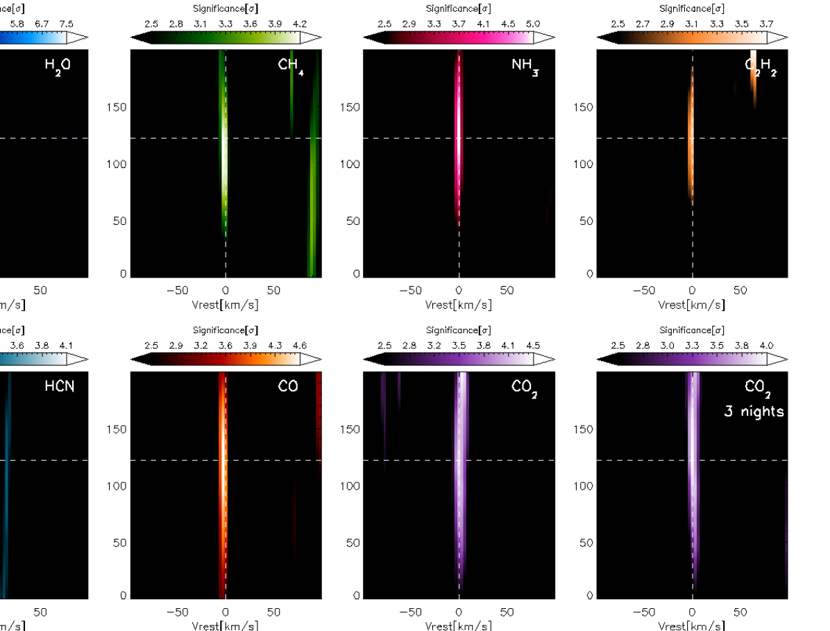
Figure 1: Significance maps of the cross-correlation between the GIANO-B spectra and the isothermal atmospheric models, as a function of the planet’s maximum radial velocity (K_P) and the planet’s rest-frame velocity (v_rest). For a better visualization, the maps do not show any signal $\textless$2.5$\sigma$. The dashed white lines indicate the known velocity for WASP-80 b (K_P=122 km s^-1, v_rest=0 km s^-1). The CO₂ map is also shown in the case of co-adding only the three nights (not including the third night). See discussion in the text (Sec. 3) and Table 2.

Likelihood analysis

After performing the cross-correlation approach, we convert the CCFs into likelihood (LH) values (Brogi & Line, 2019). Briefly, the log-likelihood function is defined as in Eq. 9 of Brogi & Line (2019):

$$\log{L}=-\frac{N}{2}\log{[s_{f}^{2}-2R(s)+s_{g}^{2}]},$$ (1)

where N is the number of spectral channels, s${}_{f}^{2}$ is the variance of the data, s${}_{g}^{2}$ the variance of the model and $R(s)$ the cross-covariance between the data and the model with $s$ being a bin/wavelength shift. This function is computed for each order and each spectrum. The final log-likelihood value is the sum of all log-likelihood functions for each night. As in Giacobbe et al. (2021), an additional free parameter, namely the line-intensity scaling factor $S$, is introduced in this framework. If the model (i.e. the strength of the spectral lines) perfectly matches the data, $S$ will be 1, that means $\log{S}$=0. Unlike in the CC (which is a normalized quantity), the line depth is important in the LH framework and the scaling factor allows us to approximate the continuum of the model as well as to take into account the effects from other species. In this framework, we calculate the significance by comparing the maximum value of the likelihood to the mean LH value in the map used as baseline.

The likelihood function is computed for each order, each observed spectrum and each night on a grid of K_P ([0, 200] km s^-1 in steps of 1 km s^-1), v_rest ([-99, 99] km s^-1 in steps of 1 km s^-1) and $\log{S}$ ([-1.1, 1.1] in steps of 0.1). Table 2 reports the v_rest, K_P and $\log{S}$ values, while Fig. 2 shows the log-likelihood confidence interval maps for each molecule maximized at the best-fit scaling factor for the model, with a zoomed v_rest interval between [-20, 20] km s^-1 for a better readability. The original version of this map is shown in Appendix B. Since in our analysis we used fixed VMRs and single-species model (meaning that the line contrast is deeper than in a mixed model), the log${S}$ values are only indicative and cannot be properly interpreted.

In this likelihood framework, we confirm four out of five molecules detected with the CC, namely H₂O, CH₄, NH₃ and HCN. As in the case of the CC approach, CO₂ is not detected in the 4-night case, showing a significant peak at low K_P values, even though a slightly less significant peak (4.28$\sigma$) is present in the likelihood map as well. Furthermore, when we exclude the third night, the peak around the planetary K_P becomes the most significant in the map (see Fig. 2).

Finally, the CO signal shows a low value of K_P in the likelihood map, which is not compatible with the nominal K_P (see Fig. 2). This low value can be due to the contamination of the stellar CO lines, which is quasi-stationary in wavelength. In fact, because of its rotation, the stellar absorption lines are distorted by the Rossiter-McLaughlin (RM) effect and, during the transit, this effect can cause spurious signals at different transit phases, and finally in the detection maps, being of the same order of magnitude of the planetary signal. Unlike other molecules, the RM effect can heavily affect the CO detection (Brogi et al., 2016). In order to investigate this contamination, we first calculate the theoretical expected $K_{\rm P}$ for the stellar atmosphere as $v\,\sin{i}$/sin(2$\pi\phi_{1}$), where $\phi_{1}$ is the phase at transit ingress (0.014 for WASP-80). We find that the expected K_P corresponding to the stellar CO is 40.4 km s^-1, which is lower than the K_P value for the LH peak. On the other hand, it is possible that our LH result might be a combination of the stellar and planetary signal, which would appear at intermediate K_P values. As an additional test, we generated a synthetic stellar spectrum with the effective temperature, $\log{\rm g}_{*}$ and metallicity values of WASP-80, from the PHOENIX spectral library (Husser et al., 2013). We convolved this spectrum to the GIANO-B resolution and calculated the CCFs and the LH using the PHOENIX spectrum to mask the stellar lines in our observed spectra. This operation did not improve the previous results, thus resulting inconclusive.

The difference between the CC and LH maps reflects the fact that, while the CC analysis is mostly sensitive to the line position and relative (i.e. line-to-line) amplitude, the LH analysis is additionally sensitive to the line shape and the line-to-wing contrast ratio. Therefore, a model that matches well the line position in CC might still be penalised in the LH analysis if the line shape/amplitude is mismatched. This is also a strong motivation for presenting both the CC and LH analyses even in the absence of a full atmospheric retrieval. While the LH is advantageous in the amount of information extracted from the spectra, it is also more demanding in terms of the accuracy of the modelling. On the other hand, the CC analysis is probably better at detecting species even with imperfect templates, which is valuable at the exploratory stage.

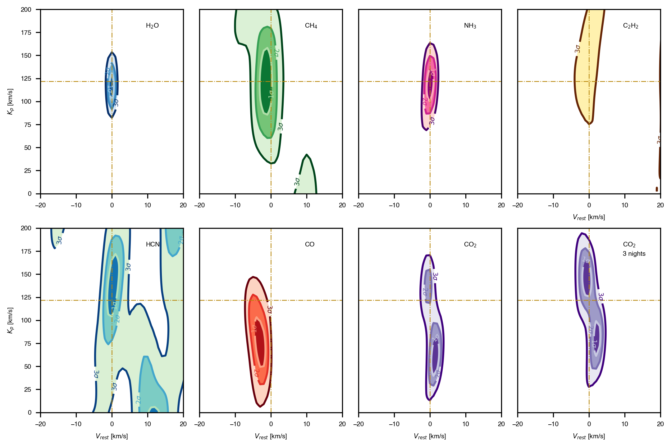
Figure 2: Likelihood confidence intervals maps for each investigated molecule as a function of K_P and v_rest and at the best-fit scaling factor. The dashed lines represent the nominal planetary velocities. As for the CC significance maps, the CO₂ likelihood map is displayed in the case of co-adding only three nights (not including the third night). As regards C₂H₂, the likelihood intervals map does not significantly change by co-adding 3 or 4 nights.

4 Atmospheric Modeling

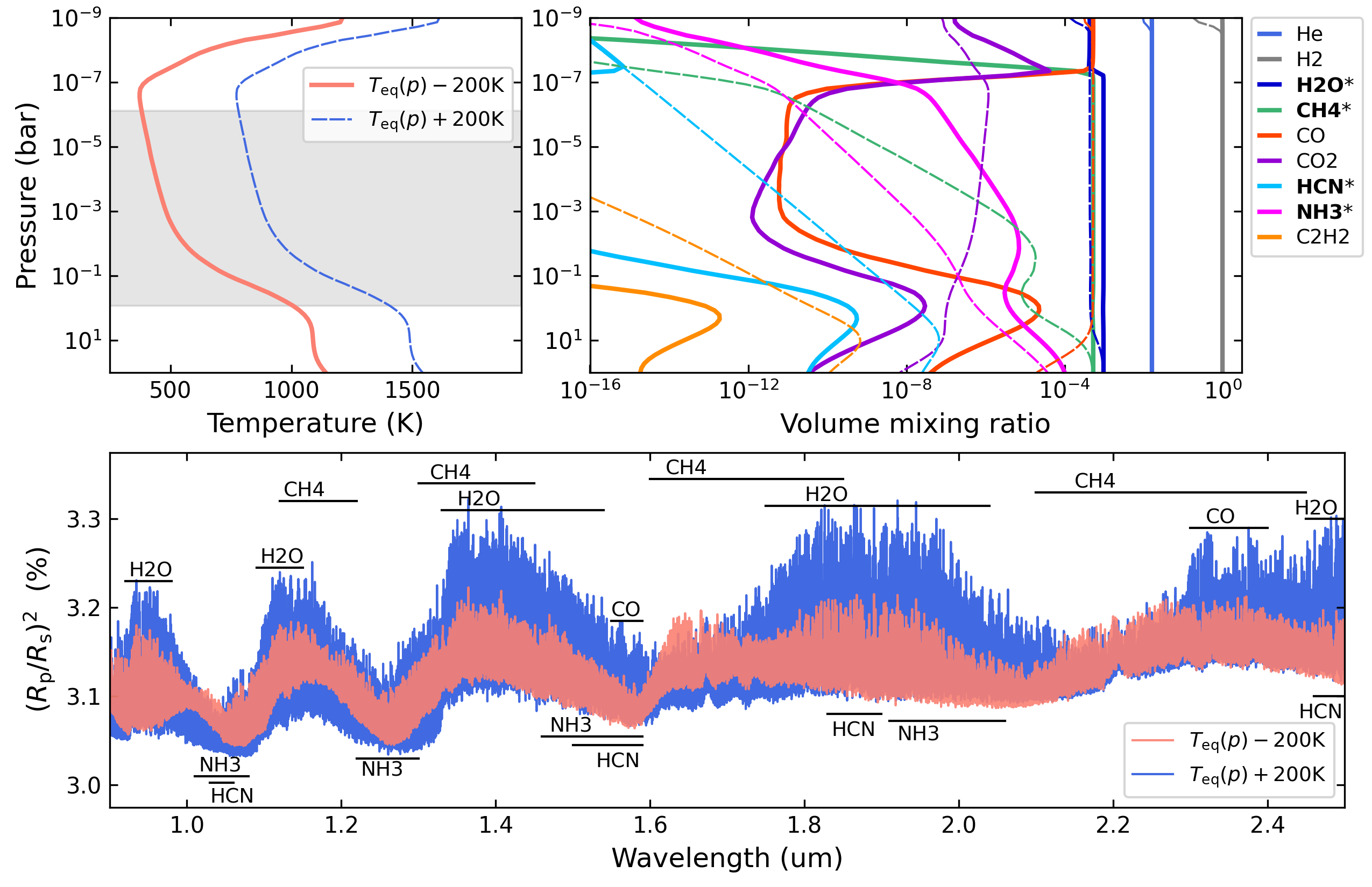
Figure 3: Sample atmospheric models for WASP-80 b in radiative and thermochemical equilibrium for a solar elemental composition. The top left panel shows the equilibrium temperature profile shifted by $\pm 200$ K, to simulate a low-temperature case (thick solid red line) and a high-temperature case (thin dashed blue line). The shaded area denotes the pressure range probed by the GIANO-B transmission observations for these models. The top right panel shows the equilibrium composition for the two temperature profiles at low (thick solid lines) and high temperature (thin dashed lines), color coded for each relevant species (see legend, with the asterisks indicating the firmly detected species). The bottom panel shows the transmission spectra over the GIANO-B wavelength range, for the low-temperature case (red) and high-temperature model (blue). The horizontal black lines denote the wavelength ranges where each of the labeled species are expected to significantly shape the transmission spectrum of WASP-80 b.

Given the rich set of molecular detections by GIANO-B on WASP-80 b, we can make rough estimates of the physical properties of the planet being guided by the observations, even without quantitative abundance estimates. In fact, WASP-80 b sits at a particularly favorably location in the parameter space to probe its temperature profile, because its equilibrium temperature straddles between two regimes where either CO ($T>T_{\rm eq}$) or CH₄ ($T<T_{\rm eq}$) dominate the carbon chemistry (e.g., Moses et al., 2013), thus making the composition particularly sensitive to the temperature profile. We therefore adopted the temperature as a main parameter to focus our exploration.

To model the atmospheric properties and theoretical spectra of WASP-80 b, we used the Pyrat Bay open-source modeling framework (Cubillos & Blecic, 2021), We explored potential physical scenarios under radiative and thermochemical equilibrium (see details in Appendix A), parameterized by the planet’s metallicity and C/O elemental ratio. Certainly, given the equilibrium temperature of WASP-80 b, processes like photochemistry or transport-induced quenching can drive the atmosphere out of chemical equilibrium (Moses, 2014). Thus, we consider the qualitative effects of disequilibrium chemistry on our models as well.

Figure 3 shows two examples of WASP-80 b models for a solar metallicity and C/O ratio, where we have shifted the equilibrium temperature profile by $\pm 200$ K, and re-computed the thermochemical equilibrium abundances and their respective transmission spectra. The variation in temperature has a significant impact in both the composition and the transmission spectra.

For the higher-temperature model CO dominates the carbon chemistry, with H₂O capturing the remaining—still largely available—oxygen (thin dashed lines). CH₄ is abundant in deeper layers, steadily decreasing with altitude. In contrast, for the lower-temperature model CH₄ dominates the carbon chemistry (solid thick lines), H₂O dominates then the oxygen chemistry, which leads to a much diminished CO abundance. Spectroscopically, both H₂O and CH₄ should present detectable absorption features in both models (having both broad absorption bands across the 0.9–2.5 m spectrum), although the spectra are mainly shaped by H₂O bands at high temperatures and CH₄ at low temperatures, due to the different relative abundances between these molecules (see bottom panel of Fig. 3).

The CO molecule, in contrast, only presents strong absorption in narrow bands (1.6 and 2.5 m) and should only be detectable in the spectrum of the higher-temperature model. A conclusive detection of CO would have favored the higher-temperature scenario, but this is not the case. The chain of reactions in the chemical network leads to drastic changes in the abundances for most other trace species as well, with CO₂, HCN, and C₂H₂ being more abundant in the higher-temperature case by several orders of magnitude. The abundance of NH₃ is somewhat decoupled from the carbon and oxygen chemistry, being more abundant at lower temperatures. At their equilibrium abundances, neither NH₃ nor HCN would present detectable features in the transmission spectra in both the low- and high-temperature models.

The detection of NH₃ and HCN would thus require to invoke disequilibrium chemistry processes that enhanced their abundances. Specifically, transport-induced quenching can drive the deep-interior abundance throughout the atmosphere, with NH₃ and CH₄ being two major species expected to be quenched. The HCN abundance can be further enhanced by a pseudo-equilibrium with the quenched CH₄ and NH₃ and be produced photochemically by stellar ultraviolet photons (see Moses, 2014, and references therein). With this in mind, both modeled cases would show evidence of NH₃ absorption when quenched from the lower layers. However, HCN would only be detectable on the higher-temperature case since its abundance at depth (from where it would be quenched) is $\sim$2 orders of magnitude larger than in the low-temperature case. Thus, the detection of HCN also points toward the higher-temperature case.

Finally, we also explored non-solar compositions. In terms of the global metallicity, CO₂ is the molecule most strongly enhanced with increasing metallicity, becoming detectable at metallicities greater than $\sim$10$\times$ solar. Thus, a confirmation of the tentative detection of CO₂ would point toward supersolar metallicities in the atmosphere of WASP-80 b. Our results for sub-solar metallicity runs (0.1$\times$) are qualitatively similar to our solar ones. In terms of C/O ratios we also considered carbon-rich atmospheres, due to the strong impact on the chemistry (e.g., Madhusudhan et al., 2011; Madhusudhan, 2012; Moses et al., 2013). We found that elemental ratios of C/O > 1 are discouraged since the H₂O abundance decreases, favoring then hydrocarbon species like CH₄, HCN, or C₂H₂.

The qualitative picture emerging from the comparison of the detected molecules with the atmospheric models we run provides tentative indications on WASP-80b’s formation history. The metallicity of the host star WASP-80 is sub-solar (Triaud et al., 2013), whereas our observations suggest a subsolar-to-solar planetary metallicity. Within this range of possibilities, if the planet had a super-stellar metallicity, combined with the solar C/O ratio estimation for WASP-80b, our observations would favour formation scenarios where the giant planet accreted a significant mass of planetesimals while migrating through its native circumstellar disc (Turrini et al., 2021a, b; Pacetti et al., 2022). While the current data do not allow to draw stronger conclusions (e.g. on the extent of WASP-80b’s migration), our NH3 detection makes WASP-80b a prime target for future efforts to quantify the abundances of C, O and N in its atmosphere and use their ratios to probe its formation history in more details (Turrini et al., 2021a, b; Kolecki & Wang, 2021; Biazzo et al., 2022; Pacetti et al., 2022). In particular, the present work will complement and help in the interpretation of JWST spectra of WASP-80 b whose transit and eclipse observations are planned through the GTO programs (PIDs 1177, 1185, and 1201).

5 Conclusions and Future Perspectives

We report on the detection of multiple molecular species in the atmosphere of the warm Jupiter, WASP-80 b, by analyzing nIR transmission spectra gathered with GIANO-B at TNG during four transits. We used two different statistical frameworks: the cross-correlation function technique and the likelihood approach. We summarize the detections as follows: we report significant detections for H₂O, CH₄, NH₃ and HCN, tentative detection for CO₂. We have inconclusive results for C₂H₂ and CO, whose presence in the WASP-80 b atmosphere cannot be either firmly confirmed or excluded (see discussion in Sec. 3), but more observations and higher S/N data will help disentangling the nature of the signals (Figures 1, 2).

The statistically robust detection of several species on WASP-80 b paves the way to estimate the chemical and physical conditions of the planet’s atmosphere. Our initial exploration considering radiative-thermochemical equilibrium models and the impact of disequilibrium processes suggest that the atmosphere is compatible with a solar composition (H₂O and CH₄ detections), possibly affected by disequilibrium chemistry (NH₃ and HCN detections). Future confirmation of the detection (or non-detection) of CO will place strong constraints on the temperature profile. Likewise, a confirmation of CO₂ will help to constrain the atmospheric metallicity.

These results demonstrate for the first time that not only hot Jupiters (Giacobbe et al., 2021), but also warm giant planets present a rich chemistry in their atmosphere, breaking new ground in the study of exoplanetary atmospheres. With recent (e.g. CRIRES+, JWST) and future upcoming (e.g., ELTs, ARIEL) instruments, it will be possible to combine multiple wavelength bands and resolutions to derive accurate and precise molecular abundances as well as atmospheric elemental ratios (e.g. the C/O, N/O and C/N ratios) and metallicity, thus confirming/updating our qualitative estimates of solar C/O and metallicity under the assumption of thermo-chemical equilibrium, and our tentative constraints on WASP-80 b’s formation history. In particular, the combined information provided by the abundance ratios of elements with different volatility, like C, O and N revealed by our detections in WASP-80b’s atmosphere, provides a direct window into the formation and migration history of giant planets (Turrini et al., 2021a, b; Kolecki & Wang, 2021). The improved estimates of the abundance of these elements achievable by such future facilities will therefore allow us to reconstruct the details of WASP-80b’s formation history.

Appendix A Radiative-equilibrium Modeling

To setup the Pyrat Bay modeling framework to attain radiative and thermochemical equilibrium, we solved the radiative-transfer equation in an iterative approach, under the two-stream, plane-parallel, local-thermodynamic, and hydrostatic approximations (following Heng et al., 2014; Malik et al., 2017). To enforce chemical equilibrium, we calculated the compositions using the thermochemical-equilibrium abundances code TEA (Blecic et al., 2016) for input elemental composition, temperature, and pressure profiles. In this work we modeled a chemical network containing H, He, C, N, O, Na, K, H₂, H₂O, CH₄, CO, CO₂, OH, C₂H₂, C₂H₄, N₂, NH₃, and HCN. Simultaneously, to enforce radiative equilibrium the code updates the temperature profile until the divergence of the upward–downward net fluxes converges to a negligible value at each layer. As boundary conditions we imposed a 100 K blackbody internal radiative heat and an incident stellar irradiation according to the properties of WASP-80, assuming zero Bond albedo and full day–night energy redistribution.

We performed the radiative-transfer calculation over a fixed pressure profile ranging from $100$ to $10^{-9}$ bar, and a wavelength grid ranging from 0.3 to 30 m sampled with a 0.3 cm^-1 spacing, sufficient to encompass the bulk of the stellar and planetary radiation (mainly in the optical and infrared, respectively). The radiative-transfer opacities include line lists for the most relevant molecular species, i.e., CO, CO₂, and CH₄ from HITEMP (Rothman et al., 2010; Li et al., 2015; Hargreaves et al., 2020) and of H₂O, HCN, NH₃, and C₂H₂ from ExoMol (Polyansky et al., 2018; Chubb et al., 2020; Yurchenko et al., 2011; Harris et al., 2006, 2008; Coles et al., 2019). To handle the billion-sized ExoMol line lists, we employed the repack algorithm (Cubillos, 2017) to extract only the dominant transitions, reducing the number of transitions by a factor of $\sim$100 without a significant impact on the resulting opacities. In addition to the molecular opacities, the Pyrat Bay code included alkali resonance-line opacities for Na and K (Burrows et al., 2000); Rayleigh opacity for H, H₂, and He (Kurucz, 1970); and collision-induced absorption for H₂–H₂ and H₂–He (Borysow et al., 2001; Borysow, 2002; Richard et al., 2012).

Appendix B Likelihood maps

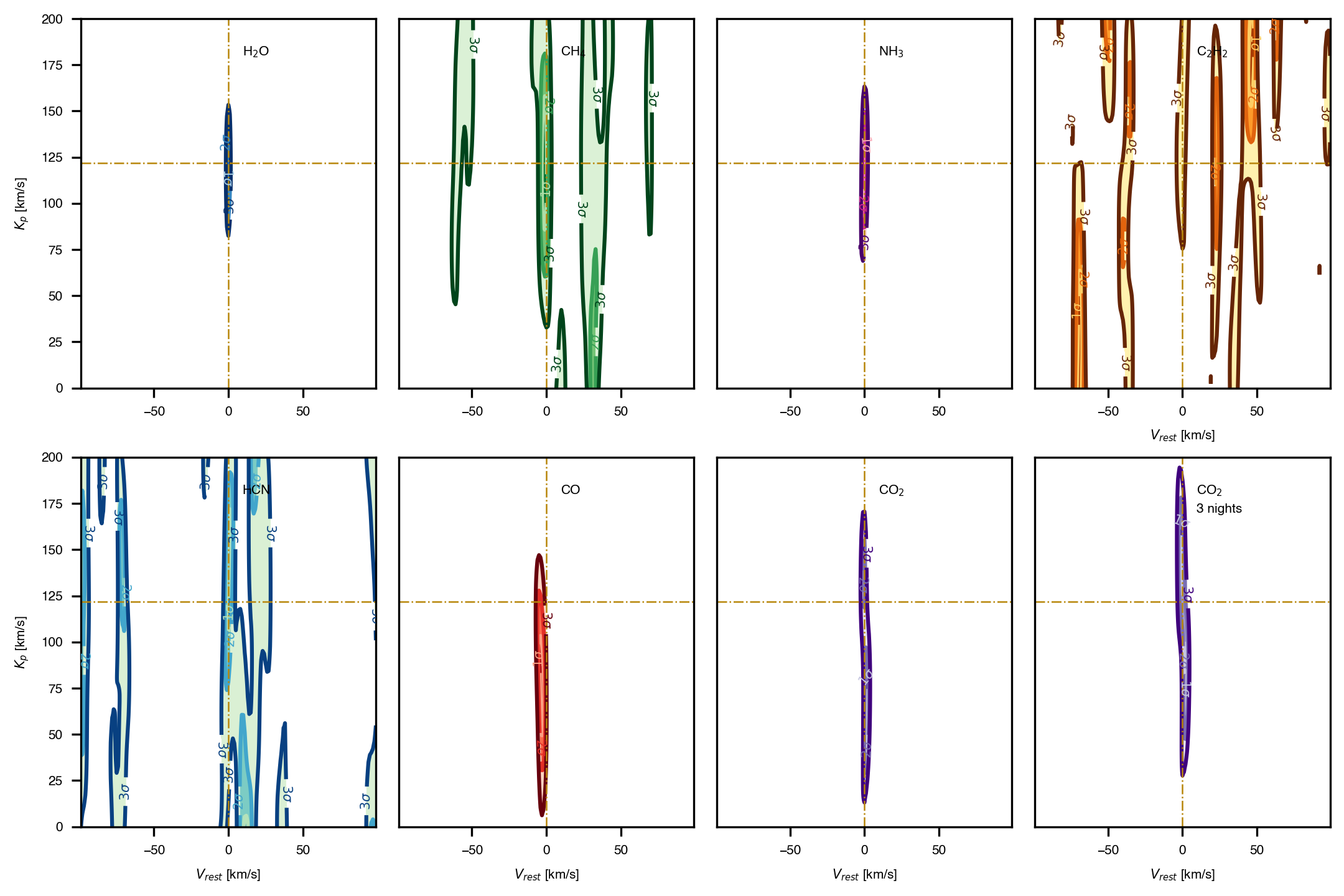
Figure 4: As Figure 2 but with v_rest interval between [-99, 99] km s^-1.

References

- Barbato et al. (2020) Barbato, D., Pinamonti, M., Sozzetti, A., et al. 2020, A&A, 641, A68, doi: 10.1051/0004-6361/202037954
- Barber et al. (2014) Barber, R. J., Strange, J. K., Hill, C., et al. 2014, Mon. Not. R. Astron. Soc., 437, 1828, doi: 10.1093/mnras/stt2011
- Biazzo et al. (2022) Biazzo, K., D’Orazi, V., Desidera, S., et al. 2022, arXiv e-prints, arXiv:2205.15796. https://arxiv.org/abs/2205.15796
- Birkby (2018) Birkby, J. L. 2018, arXiv e-prints, arXiv:1806.04617. https://arxiv.org/abs/1806.04617
- Blecic et al. (2016) Blecic, J., Harrington, J., & Bowman, M. O. 2016, ApJS, 225, 4, doi: 10.3847/0067-0049/225/1/4
- Bonomo et al. (2017) Bonomo, A. S., Desidera, S., Benatti, S., et al. 2017, A&A, 602, A107, doi: 10.1051/0004-6361/201629882
- Borsa et al. (2019) Borsa, F., Rainer, M., Bonomo, A. S., et al. 2019, A&A, 631, A34, doi: 10.1051/0004-6361/201935718
- Borysow (2002) Borysow, A. 2002, A&A, 390, 779, doi: 10.1051/0004-6361:20020555
- Borysow et al. (2001) Borysow, A., Jorgensen, U. G., & Fu, Y. 2001, J. Quant. Spec. Radiat. Transf., 68, 235, doi: 10.1016/S0022-4073(00)00023-6
- Brogi et al. (2016) Brogi, M., de Kok, R. J., Albrecht, S., et al. 2016, ApJ, 817, 106, doi: 10.3847/0004-637X/817/2/106
- Brogi & Line (2019) Brogi, M., & Line, M. R. 2019, AJ, 157, 114, doi: 10.3847/1538-3881/aaffd3
- Burrows et al. (2000) Burrows, A., Marley, M. S., & Sharp, C. M. 2000, ApJ, 531, 438, doi: 10.1086/308462
- Carleo et al. (2018) Carleo, I., Benatti, S., Lanza, A. F., et al. 2018, A&A, 613, A50, doi: 10.1051/0004-6361/201732350
- Carleo et al. (2020) Carleo, I., Malavolta, L., Lanza, A. F., et al. 2020, A&A, 638, A5, doi: 10.1051/0004-6361/201937369
- Chubb et al. (2020) Chubb, K. L., Tennyson, J., & Yurchenko, S. N. 2020, MNRAS, 493, 1531, doi: 10.1093/mnras/staa229
- Claudi et al. (2017) Claudi, R., Benatti, S., Carleo, I., et al. 2017, European Physical Journal Plus, 132, 364, doi: 10.1140/epjp/i2017-11647-9
- Coles et al. (2019) Coles, P. A., Yurchenko, S. N., & Tennyson, J. 2019, MNRAS, 490, 4638, doi: 10.1093/mnras/stz2778
- Cosentino et al. (2012) Cosentino, R., Lovis, C., Pepe, F., et al. 2012, in Society of Photo-Optical Instrumentation Engineers (SPIE) Conference Series, Vol. 8446, Ground-based and Airborne Instrumentation for Astronomy IV, ed. I. S. McLean, S. K. Ramsay, & H. Takami, 84461V, doi: 10.1117/12.925738
- Cosentino et al. (2014) Cosentino, R., Lovis, C., Pepe, F., et al. 2014, in Society of Photo-Optical Instrumentation Engineers (SPIE) Conference Series, Vol. 9147, Ground-based and Airborne Instrumentation for Astronomy V, ed. S. K. Ramsay, I. S. McLean, & H. Takami, 91478C, doi: 10.1117/12.2055813
- Cubillos (2017) Cubillos, P. E. 2017, ApJ, 850, 32, doi: 10.3847/1538-4357/aa9228
- Cubillos (2019) —. 2019, bibmanager: A BibTeX manager for LaTeX projects, Zenodo, doi:10.5281/zenodo.2547042, Zenodo, doi: 10.5281/zenodo.2547042
- Cubillos & Blecic (2021) Cubillos, P. E., & Blecic, J. 2021, MNRAS, 505, 2675, doi: 10.1093/mnras/stab1405
- Damasso et al. (2020) Damasso, M., Lanza, A. F., Benatti, S., et al. 2020, A&A, 642, A133, doi: 10.1051/0004-6361/202038864
- Fisher & Heng (2018) Fisher, C., & Heng, K. 2018, MNRAS, 481, 4698, doi: 10.1093/mnras/sty2550
- Fossati et al. (2022) Fossati, L., Guilluy, G., Shaikhislamov, I. F., et al. 2022, A&A, 658, A136, doi: 10.1051/0004-6361/202142336
- Gandhi & Madhusudhan (2017) Gandhi, S., & Madhusudhan, N. 2017, MNRAS, 472, 2334, doi: 10.1093/mnras/stx1601
- Gandhi et al. (2020) Gandhi, S., Brogi, M., Yurchenko, S. N., et al. 2020, MNRAS, 495, 224, doi: 10.1093/mnras/staa981
- Giacobbe et al. (2021) Giacobbe, P., Brogi, M., Gandhi, S., et al. 2021, Nature, 592, 205, doi: 10.1038/s41586-021-03381-x
- Guilluy et al. (2020) Guilluy, G., Andretta, V., Borsa, F., et al. 2020, A&A, 639, A49, doi: 10.1051/0004-6361/202037644
- Hargreaves et al. (2020) Hargreaves, R. J., Gordon, I. E., Rey, M., et al. 2020, ApJS, 247, 55, doi: 10.3847/1538-4365/ab7a1a
- Harris et al. (2020) Harris, C. R., Millman, K. J., van der Walt, S. J., et al. 2020, Nature, 585, 357, doi: 10.1038/s41586-020-2649-2
- Harris et al. (2008) Harris, G. J., Larner, F. C., Tennyson, J., et al. 2008, MNRAS, 390, 143, doi: 10.1111/j.1365-2966.2008.13642.x
- Harris et al. (2006) Harris, G. J., Tennyson, J., Kaminsky, B. M., Pavlenko, Y. V., & Jones, H. R. A. 2006, Mon. Not. R. Astron. Soc., 367, 400, doi: 10.1111/j.1365-2966.2005.09960.x
- Heng et al. (2014) Heng, K., Mendonça, J. M., & Lee, J.-M. 2014, ApJS, 215, 4, doi: 10.1088/0067-0049/215/1/4
- Hood et al. (2020) Hood, C. E., Fortney, J. J., Line, M. R., et al. 2020, AJ, 160, 198, doi: 10.3847/1538-3881/abb46b
- Huang et al. (2013) Huang, X., Freedman, R. S., Tashkun, S. A., Schwenke, D. W., & Lee, T. J. 2013, J. Quant. Spec. Radiat. Transf., 130, 134, doi: 10.1016/j.jqsrt.2013.05.018
- Huang et al. (2017) Huang, X., Schwenke, D. W., Freedman, R. S., & Lee, T. J. 2017, Journal of Quantitative Spectroscopy and Radiative Transfer, 203, 224 , doi: https://doi.org/10.1016/j.jqsrt.2017.04.026
- Hunter (2007) Hunter, J. D. 2007, Computing In Science & Engineering, 9, 90, doi: 10.1109/MCSE.2007.55
- Husser et al. (2013) Husser, T. O., Wende-von Berg, S., Dreizler, S., et al. 2013, A&A, 553, A6, doi: 10.1051/0004-6361/201219058
- Kirk et al. (2018) Kirk, J., Wheatley, P. J., Louden, T., et al. 2018, MNRAS, 474, 876, doi: 10.1093/mnras/stx2826
- Kolecki & Wang (2021) Kolecki, J. R., & Wang, J. 2021, arXiv e-prints, arXiv:2112.02031. https://arxiv.org/abs/2112.02031
- Kurucz (1970) Kurucz, R. L. 1970, SAO Special Report, 309
- Li et al. (2015) Li, G., Gordon, I. E., Rothman, L. S., et al. 2015, ApJS, 216, 15, doi: 10.1088/0067-0049/216/1/15
- López-Morales & Seager (2007) López-Morales, M., & Seager, S. 2007, ApJ, 667, L191, doi: 10.1086/522118
- Madhusudhan (2012) Madhusudhan, N. 2012, ApJ, 758, 36, doi: 10.1088/0004-637X/758/1/36
- Madhusudhan (2019) —. 2019, ARA&A, 57, 617, doi: 10.1146/annurev-astro-081817-051846
- Madhusudhan et al. (2011) Madhusudhan, N., Harrington, J., Stevenson, K. B., et al. 2011, Nature, 469, 64, doi: 10.1038/nature09602
- Malik et al. (2017) Malik, M., Grosheintz, L., Mendonça, J. M., et al. 2017, AJ, 153, 56, doi: 10.3847/1538-3881/153/2/56
- Mancini et al. (2014) Mancini, L., Southworth, J., Ciceri, S., et al. 2014, A&A, 562, A126, doi: 10.1051/0004-6361/201323265
- Mansfield et al. (2021) Mansfield, M., Line, M. R., Bean, J. L., et al. 2021, Nature Astronomy, 5, 1224, doi: 10.1038/s41550-021-01455-4
- Meurer et al. (2017) Meurer, A., Smith, C. P., Paprocki, M., et al. 2017, PeerJ Computer Science, 3, e103, doi: 10.7717/peerj-cs.103
- Moses (2014) Moses, J. I. 2014, Philosophical Transactions of the Royal Society of London Series A, 372, 20130073, doi: 10.1098/rsta.2013.0073
- Moses et al. (2013) Moses, J. I., Madhusudhan, N., Visscher, C., & Freedman, R. S. 2013, ApJ, 763, 25, doi: 10.1088/0004-637X/763/1/25
- Oliva et al. (2006) Oliva, E., Origlia, L., Baffa, C., et al. 2006, in Society of Photo-Optical Instrumentation Engineers (SPIE) Conference Series, Vol. 6269, Society of Photo-Optical Instrumentation Engineers (SPIE) Conference Series, ed. I. S. McLean & M. Iye, 626919, doi: 10.1117/12.670006
- Pacetti et al. (2022) Pacetti, E., Turrini, D., Schisano, E., et al. 2022, arXiv e-prints, arXiv:2206.14685. https://arxiv.org/abs/2206.14685
- Parviainen et al. (2018) Parviainen, H., Pallé, E., Chen, G., et al. 2018, A&A, 609, A33, doi: 10.1051/0004-6361/201731113
- Pérez & Granger (2007) Pérez, F., & Granger, B. E. 2007, Computing in Science and Engineering, 9, 21, doi: 10.1109/MCSE.2007.53
- Pino et al. (2020) Pino, L., Désert, J.-M., Brogi, M., et al. 2020, ApJ, 894, L27, doi: 10.3847/2041-8213/ab8c44
- Polyansky et al. (2018) Polyansky, O. L., Kyuberis, A. A., Zobov, N. F., et al. 2018, MNRAS, 480, 2597, doi: 10.1093/mnras/sty1877
- Rainer et al. (2018) Rainer, M., Harutyunyan, A., Carleo, I., et al. 2018, in Society of Photo-Optical Instrumentation Engineers (SPIE) Conference Series, Vol. 10702, Ground-based and Airborne Instrumentation for Astronomy VII, ed. C. J. Evans, L. Simard, & H. Takami, 1070266, doi: 10.1117/12.2312130
- Richard et al. (2012) Richard, C., Gordon, I. E., Rothman, L. S., et al. 2012, J. Quant. Spec. Radiat. Transf., 113, 1276, doi: 10.1016/j.jqsrt.2011.11.004
- Rothman et al. (2010) Rothman, L. S., Gordon, I. E., Barber, R. J., et al. 2010, JQSRT, 111, 2139, doi: 10.1016/j.jqsrt.2010.05.001
- Sedaghati et al. (2017) Sedaghati, E., Boffin, H. M. J., Delrez, L., et al. 2017, MNRAS, 468, 3123, doi: 10.1093/mnras/stx646
- Sing et al. (2016) Sing, D. K., Fortney, J. J., Nikolov, N., et al. 2016, Nature, 529, 59, doi: 10.1038/nature16068
- Tennyson et al. (2016) Tennyson, J., Yurchenko, S. N., Al-Refaie, A. F., et al. 2016, Journal of Molecular Spectroscopy, 327, 73, doi: 10.1016/j.jms.2016.05.002
- Triaud et al. (2013) Triaud, A. H. M. J., Anderson, D. R., Collier Cameron, A., et al. 2013, A&A, 551, A80, doi: 10.1051/0004-6361/201220900
- Triaud et al. (2015) Triaud, A. H. M. J., Gillon, M., Ehrenreich, D., et al. 2015, MNRAS, 450, 2279, doi: 10.1093/mnras/stv706
- Tsiaras et al. (2018) Tsiaras, A., Waldmann, I. P., Zingales, T., et al. 2018, AJ, 155, 156, doi: 10.3847/1538-3881/aaaf75
- Turrini et al. (2021a) Turrini, D., Schisano, E., Fonte, S., et al. 2021a, ApJ, 909, 40, doi: 10.3847/1538-4357/abd6e5
- Turrini et al. (2021b) Turrini, D., Codella, C., Danielski, C., et al. 2021b, Experimental Astronomy, doi: 10.1007/s10686-021-09754-4
- Virtanen et al. (2020) Virtanen, P., Gommers, R., Oliphant, T. E., et al. 2020, Nature Methods, 17, 261, doi: 10.1038/s41592-019-0686-2
- Welch (1947) Welch, B. L. 1947, Biometrika, 34, 28. http://www.jstor.org/stable/2332510
- Yurchenko et al. (2011) Yurchenko, S. N., Barber, R. J., & Tennyson, J. 2011, MNRAS, 413, 1828, doi: 10.1111/j.1365-2966.2011.18261.x