The GAPS Programme at TNG

Abstract

Context.

Aims. The field of exo-atmospheric characterisation is progressing at an extraordinary pace. Atmospheric observations are now available for tens of exoplanets, mainly hot and warm inflated gas giants, and new molecular species continue to be detected revealing a richer atmospheric composition than previously expected. Thanks to its warm equilibrium temperature (963$\pm$18 K) and low-density (0.219$\pm$0.031 g cm^-3), the close-in gas giant WASP-69b represents a golden target for atmospheric characterisation.

Methods. With the aim of searching for molecules in the atmosphere of WASP-69b and investigating its properties, we performed high-resolution transmission spectroscopy with the GIANO-B near-infrared spectrograph at the Telescopio Nazionale Galileo.

Results. We observed three transit events of WASP-69b. During a transit, the planetary lines are Doppler-shifted due to the large change in the planet’s radial velocity, allowing us to separate the planetary signal from the quasi-stationary telluric and stellar spectrum.

Conclusions. Considering the three nights together, we report the detection of CH₄, NH₃, CO, C₂H₂, and H₂O, at more than $3.3\sigma$ level. We did not identify the presence of HCN and CO₂ with confidence level higher than 3$\sigma$. This is the first time that five molecules are simultaneously detected in the atmosphere of a warm giant planet. These results suggest that the atmosphere of WASP-69b is possibly carbon-rich and characterised by the presence of disequilibrium chemistry.

1 Introduction

Ground-based, high-resolution (resolving power $R\geq$20 000) spectroscopy (HRS) in the near-infrared (nIR) represents an effective approach to investigate exoplanet atmospheres. Indeed, at high spectral resolution, thousands of resolved molecular lines can be disentangled, as they are Doppler shifted by tens of km s^-1 due to the planet motion along its orbit from the telluric (Earth’s atmosphere) and stellar lines that are (quasi-)stationary in wavelength.

Hot ($T_{\rm eq}>1000$ K) and warm ($T_{\rm{eq}}\leq 1000$ K) inflated giant planets are the most suitable targets for atmospheric characterisation (Seager & Deming 2010). Recently, Giacobbe et al. (2021) reported the simultaneous detection of six molecules in the atmosphere of one of the best-studied hot-Jupiters (HJs), HD 209458b. As only two molecules (CO and H₂O) had been detected at the same time in exoplanetary atmospheres in the past (e.g., Tsiaras et al. 2018), the work presented in Giacobbe et al. (2021) revealed a previously unknown chemical complexity. Thus this discovery raises the question of whether the complexity of HD 209458b’s atmosphere is unique or other exo-atmospheres show such a rich molecular composition. Such molecular diversity enables one to derive atmospheric abundances and thus elemental ratios, such as Carbon-to-Oxygen (C/O) ratio, can then be obtained, allowing us to derive important clues on the formation and migration histories of hot giant planets (e.g., Madhusudhan 2012; Turrini et al. 2021b). For example Giacobbe et al. (2021) retrieved a C/O ratio $\geq$ 1, meaning that HD 209458b formed far from its present location and subsequently migrated inwards.
With a warm temperature and low density (see Table 1), the close-in transiting planet WASP-69b represents a suitable laboratory for atmospheric characterization studies. Furthermore, the low equilibrium temperature T${}_{\mathrm{eq}}\leq$1000 K places the planet in a different regime compared to that of the HJ HD 209458b (T${}_{\rm{eq}}\sim$1500 K): the equilibrium chemistry shifts in favour of CH₄ rather than CO and disequilibrium phenomena (i.e. vertical mixing and photochemical processes) are more likely to alter the molecular abundances compared to the atmospheres of hotter planets (e.g., Moses 2014).

The atmosphere of WASP-69b has been studied with both space-based low-resolution (LR) and ground-based high-resolution (HR) in-transit (transmission spectroscopy) observations. LR observations performed with WFC3 on board the Hubble Space Telescope (HST) unveiled the presence of H₂O and possibly aerosols (Tsiaras et al. 2018; Fisher & Heng 2018). Sodium has also been detected through HR optical observations (e.g., Casasayas-Barris et al. 2017). Moreover, HR and LR observations covering the nIR He I (1083.3 nm) revealed that the planet has an extended and escaping atmosphere, where the escape is driven by the intense X-ray and extreme ultraviolet radiation received from the active K5V host star (e.g., Nortmann et al. 2018; Vissapragada et al. 2020).

In this work, we present transmission spectroscopy of WASP-69b using HR observations in the nIR, searching for the absorption of multiple molecular species. We observed the WASP-69 system within the long-term observing program at the Telescopio Nazionale Galileo (TNG) telescope “GAPS2: the origin of planetary systems” -awarded to the Italian GAPS (Global Architecture of Planetary System) Collaboration (Poretti et al. 2016). Part of this program is devoted to the characterisation of exoplanetary atmospheres at HR. Briefly, we are carrying out transmission and emission spectroscopy of 26 hot Jupiters and 4 hot Neptunes and/or sub-Neptunes in a wide range of T_eq (625-2500 K), and hosted by stars of different spectral types (A to M with $K<10.5$ mag) to ($i$) identify atomic species to estimate the abundance of refractory elements (Pino et al. 2020) and/or to probe atmospheric expansion/escape, for instance from the H$\alpha$ (Borsa et al. 2021) and/or metastable Helium triplet (Guilluy et al. 2019); ($ii$) detect molecular compounds and estimate the atmospheric C/O ratio and metallicity, which in turn provide constraints on the planet formation and evolution scenarios (Giacobbe et al. 2021); ($iii$) derive temperature-pressure profiles (Pino et al. 2020; Borsa et al. 2022); ($iv$) detect the atmospheric Rossiter-McLaughlin effect (Borsa et al. 2019; Rainer et al. 2021).
Fig. 1 places WASP-69b into the broader context of the GAPS atmospheric survey. The symbol size is proportional to the expected atmospheric signal in the K band:

$$S/N=\frac{2HR_{P}}{R_{\star}^{2}}*\sqrt{F},$$ (1)

where we account for the stellar magnitude in K band ($F=10^{-\frac{magK}{2.5}}$), the atmospheric scale height ($H$), the planetary ($R_{P}$) and the stellar radius ($R_{\star}$). The most suitable targets to perform atmospheric characterisation studies are labelled. As this plot shows, WASP-69b represents one of the best suitable candidates to perform atmospheric studies (2R_PH/R${}_{\star}^{2}\sim$ 283 ppm, Brown et al. 2001 ) in the temperature range ($\leq$1000 K) we aimed to probe within this study.

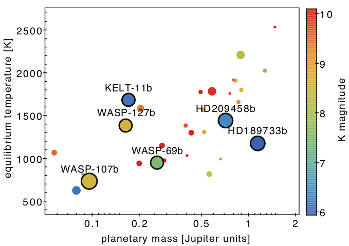
Figure 1: Mass-equilibrium temperature relation for the planets within the GAPS atmospheres survey. The symbol size is proportional to the expected atmospheric signal (for one scale height) in K band.The six more suitable targets to perform atmospheric characterisation studies are labelled.

Table 1: Physical and orbital parameters of the WASP-69 system adopted in this work.

Orbital parameters
Orbital Period - P[days]	3.8681382(17)	1,2
Mid Transit time - Tc[BJDTDB]	2455748.83422(18)	1,2
Semi-major axis - a[au]	0.04527${}^{+0.00053}_{-0.00054}$	1
Orbital inclination - i[deg]	86.71(20)	1,2
Systemic velocity - Vsys[km/s]	-9.37(21)	3
Transit Duration - T14[h]	2.2296(288)	2
Radial-velocity semi-amplitude - KP[km/s]	127.11${}^{+1.49}_{-1.52}$	This paper*
Orbital eccentricity - e	¡ 0.11	1
Transit ingress/egress - $\phi_{1}$	0.01201(16)	This paper°
Planetary Parameters
Mass - MP[MJup]	0.260(17)	2
Radius - RP[RJup]	1.057(47)	2
Equilibrium Temperature - Teq[K]	963(18)	2
Density - $\rho_{\mathrm{P}}$[kg m-3]	219000(31000)	2
Stellar Parameters
Mass - M⋆[M⊙]	0.826(29)	2
Radius - R⋆[R⊙]	0.813(28)	2
Effective Temperature - T⋆[K]	4715(50)	2
Spectral Type	KV5	2
Index color - B-V	1.06	4
Stellar Rotational velocity - vsini[km/s]	2.20(40)	1,2

• ^∗Derived from $a$, $P$, and $i$ as $\frac{2\pi a}{P}\sin{i}$,
  ⁺Derived from HARPS-N,
  ^oOrbital phase corresponding to transit ingress/egress derived as $\frac{T_{14}}{2\,P}$

• References: ⁽¹⁾Bonomo et al. (2017), ⁽²⁾Anderson et al. (2014), ⁽³⁾Gaia DR2 (Gaia Collaboration et al. 2018), ⁽⁴⁾From the Tycho-2 catalogue (Høg et al. 2000),

This letter is organized as follows: in Sect. 2 we present the data we collected, in Sect. 3 we describe the analysis that we performed to extract the planetary transmission spectrum and, therefore, the molecules responsible for absorption, from the raw GIANO-B data. Finally, we discuss our results and draw the conclusions in Sect. 4.

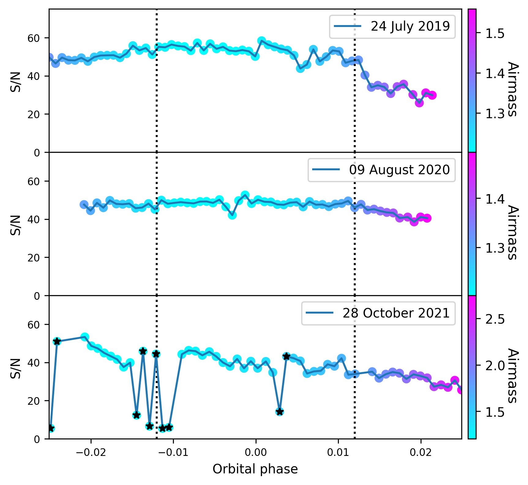
Figure 2: Average S/N across the entire GIANO-B spectral range as a function of the orbital phase, with the marker color indicating the airmass at which the observations have been gathered. Ingress and egress of WASP-69b ($\phi_{1}$ in Table 1) are marked with vertical dashed lines. Black stars on the last night (October 28, 2021) indicate the discarded AB couples for low S/N.

2 Data sample

We observed the WASP-69 system with the TNG telescope in GIARPS configuration by simultaneously measuring HR spectra in the optical (0.39-0.69 $\mu$m) and nIR (0.95-2.45 $\mu$m) with the HARPS-N ($R\approx 115\,000$) and GIANO-B (R$\sim$50,000) spectrographs. Our data encompass a total of three primary transits of WASP-69 b, which were obtained at UT 24 July 2019, UT 09 August 2020 and UT 28 October 2021. The GIANO-B observations were taken according to an ABAB nodding pattern (Claudi et al. 2017) for an optimal subtraction of the thermal background noise and telluric emission lines. The observations consist of spectra taken before, during, and after the planetary transit; Fig. 2 shows the signal-to-noise ratio (S/N) averaged over the entire GIANO-B spectral coverage as a function of the planet’s orbital phase and of the airmass for each of the three nights. The observations during the last night (October 28, 2021) were affected by several thin clouds (cirri), so we decided to discard the AB couples of observations which exhibit a very low S/N compared to the others (lowest S/N in the couple less then 15, see Fig. 2). A log of the observations is reported in Table 3.

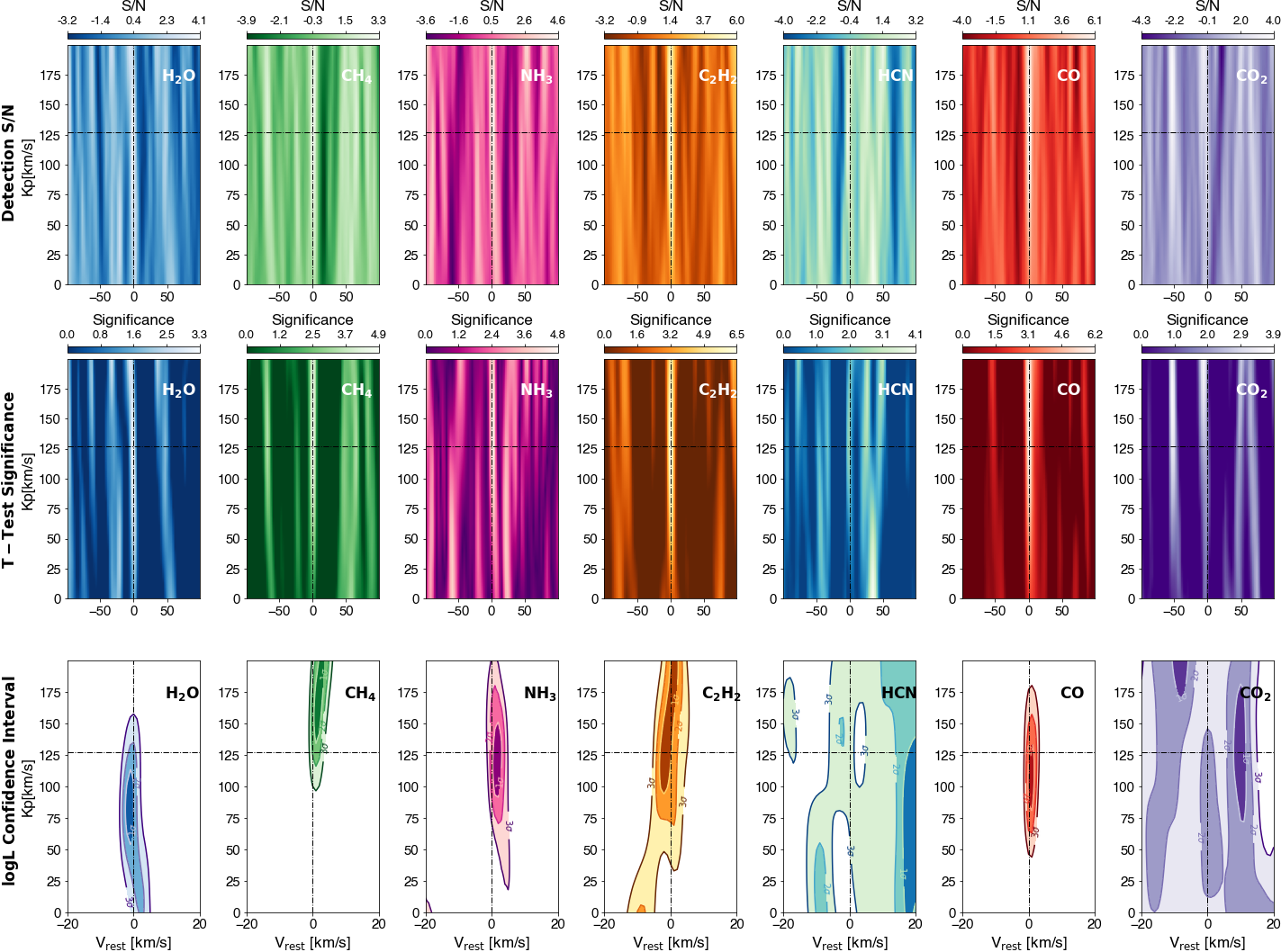
Figure 3: CC both in the S/N (top panel) and in the significance (middle panel) framework, and LH confidence intervals (bottom panel) maps for each investigated molecules as a function of the planet’s maximum radial velocity ($K_{\mathrm{P}}$) and the planet’s rest-frame velocity ($V_{\mathrm{rest}}$). The dotted lines denote the expected radial-velocity semi-amplitude of WASP-69b ($K_{\mathrm{P}}$=127.11${}^{+1.49}_{-1.52}$ km s^-1) in the planet rest-frame ($V_{\mathrm{rest}}$=0 km s^-1). The detection significance increased when transits are co-added.

3 Data Analysis

Here we report the steps we performed in order to recover the planetary signal from the GIANO-B raw images.

($i$) Basic data reduction. We processed the raw GIANO-B spectra with the GOFIO pipeline (Rainer et al. 2018) to perform flat-fielding, bad pixel correction, background subtraction, optimal extraction of the 1-d spectra, and a preliminary wavelength calibration using an Uranium-Neon lamp. We corrected small temporal variations in the wavelength solution due to non-perfect stability of the spectrograph (Giacobbe et al. 2021), and refined the initial wavelength solution by employing a HR transmission spectrum of the Earth’s atmosphere generated via the ESO Sky Model Calculator. As some spectral regions have too many or too few telluric lines, this calibration refinement was not possible for all the orders (e.g., Brogi et al. 2018; Guilluy et al. 2019; Fossati et al. 2022). We report in Table 4 the discarded orders for each individual night of observation.

($ii$) Telluric and stellar Lines Removal. We then removed the telluric contamination and the stellar spectrum by employing the Principal Component Analysis (PCA) and linear regression techniques (Giacobbe et al. 2021). We selected the optimal number of components $N_{\mathrm{opt}}$ following the procedure described in Giacobbe et al. (2021). More precisely, $N_{\mathrm{opt}}$ varies with the considered order depending on the Root Mean Square (rms) variation. We selected the number for which the first derivative between the last and penultimate component decreases by less than $\sigma_{\mathrm{white}}N_{\mathrm{opt}}^{-1/2}$, where $\sigma_{\mathrm{white}}$ is the standard deviation of the full matrix assuming pure white noise. Since in two nights out of three (i.e., UT 24 July 2019, and UT 09 August 2020) the relative velocity shift between telluric and planetary lines was close to zero, we masked the telluric components to avoid contamination in our final spectra. Following Brogi et al. (2018), we thus masked the data assigning zero flux to those spectral channels corresponding to telluric lines deeper than 20$\%$. Finally, we visually inspected the outcome for spurious telluric residuals.

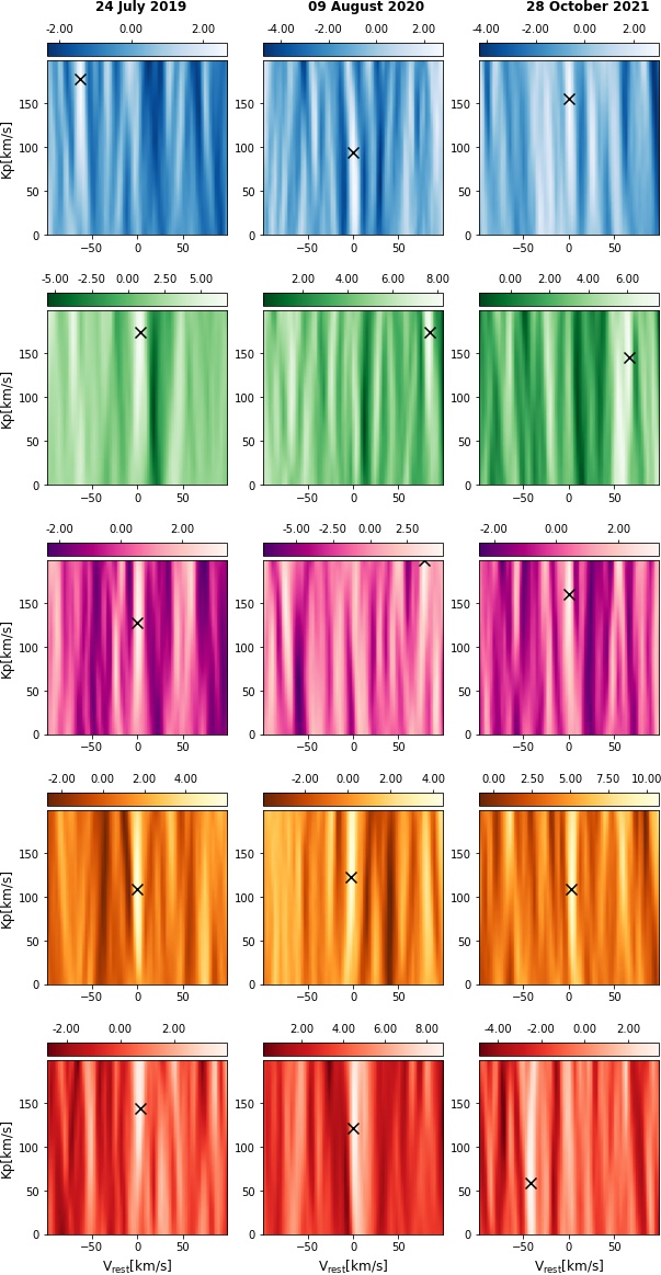
Figure 5: S/N maps for the detected molecules for each night considered individually. The CC peaks are indicated by a black cross. As discussed in Giacobbe et al. (2021), species have weaker signatures and are not always detected in each individual transit. Nevertheless, they are firmly detected when more transits are co-added. These results show the advantage of our multi-night approach.

($iii$) Search for molecules through cross-correlation. For each considered molecule, we combined the contribution of thousands of lines in the spectral coverage of GIANO-B by performing the cross-correlation (CC) of the residual spectra with isothermal transmission models generated using the GENESIS code (Gandhi & Madhusudhan 2017) adapted for transmission spectroscopy (Pinhas et al. 2018) (see Table 2 for the adopted line list). Prior to CC, the models were convolved to the GIANO-B instrument profile (a Gaussian profile with FWHM 5.4 km s^-1). Models were calculated between 100 and 10^-8 bar in pressure, at a T${}_{\mathrm{eq}}=963(18)$K, between 0.9 and 2.6$\mu$m, with a constant spacing of 0.01 cm^-1. We included collision-induced absorption from H₂-H₂ and H₂-He interactions (Richard et al. 2012). For each night we performed the CC for an optimal selection of GIANO-B orders (Giacobbe et al. 2021) and every phase over a lag vector corresponding to planet RVs in the range $-252\leq{\rm RV}\leq 252$ km s^-1, in steps of 3 km s^-1. This range was chosen in order to cover all possible radial velocities of the planet. We then co-added the CC functions over the selected orders, nights and the orbital phase after shifting them in the planet rest-frame by assuming a circular orbit (e.g., Brogi et al. 2012, 2014, 2018). In doing so, we considered a range of planet radial-velocity semi-amplitudes $0\leq K_{\rm p}\leq 200$ km s^-1, in steps of 1.5 km s^-1. We then quantified the confidence level of our detection by computing the S/N detection map (e.g., Brogi et al. 2012, 2014, 2018). For each investigated molecule, we divided the total CC matrix by its standard deviation (calculated by excluding the CC peak). We also used the Welch t-test to compare the ‘in-trail’ values (CC values that carry signal) of the 2-d CC matrix aligned in the planet rest-frame to those ‘out-of-trail’ (CC values away from the WASP-69b’s radial velocity). We then converted the corresponding t-value into the statistical significance at which these two distributions are not drawn from the same parent distribution. We applied this method for the same range of rest-frame velocity $V{{}_{\mathrm{rest}}}$ and the planetary semi-amplitude $K{{}_{\mathrm{P}}}$ adopted before. The final S/N and significance maps for the three nights combined together are shown in the upper and in the middle panels of Fig. 3, respectively. These results show the advantage of a multi-night approach, indeed even if the data quality does not allow to always detect the signal in each individual night (see Fig. 5), the detection significance increased when transits are co-added.
The detections in CC have been obtained with isothermal models of one molecule at a time with a Volume Mixing Ratio (VMR) large enough to reveal a given molecule, if present in the atmosphere; it has been indeed demonstrated (e.g., Gandhi et al. 2020) that the CC is only weakly dependent on the absolute VMR. As a good compromise we found a VMR$\sim$10^-4.

($iv$) Confidence Intervals via Likelihood. The CC framework as applied in the previous analysis implicitly assumes that the signal amplitude and the S/N are uniform across the considered spectral range. However, this assumption is only valid at a first-order level. To investigate this aspect more thoroughly, we converted the CC values into Likelihood (LH) Mapping values using the approach proposed by Brogi & Line (2019) and used by Giacobbe et al. (2021). In this formalism, the LH is indeed set up by taking into account the model’s line depth and the S/N order by order and spectrum by spectrum. Retrieving a peak in the LH at the correct position of the ($V_{\mathrm{rest}}$, $K_{\mathrm{P}}$) space is hence an additional confirmation of our detection. We thus computed a log-LH function for each selected order, each spectrum, and each radial-velocity shift of the model across the $K_{\mathrm{P}}$ vs $V_{\mathrm{rest}}$ space. We used a lag vector corresponding to planet radial velocities (RVs) in the range $-20\leq{\rm RV}\leq 20$ km s^-1, in steps of 1 km s^-1. To take into account any possible modification of the planetary signal due to the PCA process, we performed on each theoretical model the exact telluric removal process applied to the observations. The final log-likelihood for each ($V_{\mathrm{rest}}$, $K_{\mathrm{P}}$) couple is obtained by adding all the log-LHs over each order, each night, and each observed spectrum.

Subsequently, as in Giacobbe et al. (2021), we introduced the line-intensity scaling factor $S$ ($-1.1$¡$\log{S}$¡$1.1$, in steps of 0.1), to understand how much the used models have to be scaled to match the observed data. For a model perfectly matching the data, $S$ is exactly 1 ($\log{S}$=0), i.e. the model and the data have the same average line amplitude compared to the local continuum. Scaling factors smaller than 1 indicate that spectral lines are too strong compared to the observations and, for example, the presence of a grey-cloud model can be invoked to account for that, as in Giacobbe et al. (2021). Furthermore, as in the single species models the continuum can be approximate, the introduction of the $\log{S}$ allows us to account for the muting effects of other species. On the contrary in the CC framework, as the line depth does not enter in the calculation, the $\log{S}$ is it not necessary. We then converted the LH values into confidence intervals by using the LH-ratio test between the maximum log-LH and each LH value in the ($V_{\mathrm{rest}}$, $K_{\mathrm{P}}$, $\log{S}$) space. The LH confidence intervals maps corresponding to the $\log{S}$ maximising the detection, are shown in the bottom panel of Fig. 3.

We then evaluated the significance of our LH detection by performing a LH-ratio test between the maximum log-LH and the median of the 2-d log-LH matrix values for the best-fit scaling factor which exhibited a statistical confidence greater than 1. For each considered molecule, Table 2 reports the results of our analysis in both the CC and the LH frameworks. We consider a molecule as detected if altogether the S/N, the detection significance and the LH significance are higher than 3$\sigma$.

Table 2: CC and LH results.

CC framework

LH framework

S/N map

Significance map

Confidence Intervals map

Mol

Line list

Status

$\mathbf{V{{}_{\mathrm{\mathbf{rest}}}}_{0}}$ [km/s]

Kp0 [km/s]

S/N

$\mathbf{V{{}_{\mathrm{\mathbf{rest}}}}_{0}}$ [km/s]

Kp0 [km/s]

$\sigma$

$\mathbf{V{{}_{\mathrm{\mathbf{rest}}}}_{0}}$ [km/s]

Kp0 [km/s]

$\log{S}$

$\sigma$

H2O

POKAZATEL/ExoMol

✓

0.0${}^{+3.0}_{-3.0}$

114.0${}^{+58.5}_{-57.0}$

4.1

0.0${}^{+3.0}_{-3.0}$

111.0${}^{+67.5}_{-82.5}$

3.3

-1.0${}^{+1.0}_{-2.0}$

84.0${}^{+30.0}_{-31.5}$

-0.6

5.0

CH4

HITEMP

✓

0.0${}^{+3.0}_{-3.0}$

130.5${}^{+69.0}_{-67.5}$

3.3

0.0${}^{+3.0}_{-3.0}$

132.0${}^{+67.5}_{-60.0}$

4.9

2.0${}^{+1.0}_{-1.0}$

171.0${}^{+29.0}_{-30.0}$

-0.1

6.3

NH3

CoYuTe/ExoMol

✓

0.0${}^{+3.0}_{-3.0}$

148.5${}^{+51.0}_{-57.0}$

4.6

0.0${}^{+3.0}_{-3.0}$

154.5${}^{+45.0}_{-58.5}$

4.8

2.0${}^{+1.0}_{-2.0}$

121.5${}^{+30.0}_{-31.5}$

-0.3

5.4

C2H2

ACeTY/ExoMol

✓

0.0${}^{+3.0}_{-3.0}$

130.5${}^{+52.5}_{-52.5}$

6.0

0.0${}^{+3.0}_{-3.0}$

129.0${}^{+60.0}_{-52.5}$

6.5

-2.0${}^{+2.0}_{-1.0}$

123.0${}^{+33.0}_{-30.0}$

-0.2

4.5

HCN

Harris/ExoMol

✗

CO

HITEMP

✓

0.0${}^{+3.0}_{-3.0}$

148.5${}^{+51.0}_{-69.0}$

6.1

0.0${}^{+3.0}_{-3.0}$

165.0${}^{+34.5}_{-81.0}$

6.2

1.0${}^{+1.0}_{-1.0}$

108.0${}^{+28.5}_{-28.5}$

0.1

7.0

CO2

Ames

✗

• Notes: From left to right: the investigated molecule, the adopted line list, the CC result with theoretical models both in the S/N and the significance framework, the LH findings, and the status of the detection (with ✓and ✗, indicating a detection and a non-detection, respectively). For each framework, the planet orbital semi-amplitude (Kp₀), the velocity in the planet rest-frame ($V{{}_{\mathrm{rest}}}_{0}$) of the CC/LH peak are reported. The S/N, the significance ($\sigma$), and the scaling factor ($\log{S}$) maximising the detection are also present. We used a grid of $\log{S}$ values, thus they are shown without an error bar.

• References: ,, , , , ,

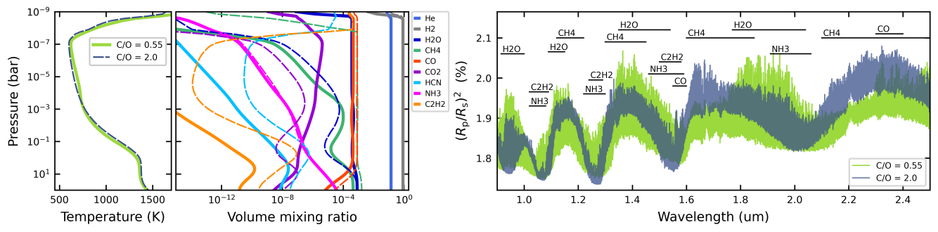
Figure 4: Sample atmospheric models for WASP-69b in radiative and thermochemical equilibrium. The left panel shows the equilibrium temperature profile for two models with solar elemental metallicity and a solar C/O ratio (solid green curve) or a super-solar ratio (dashed blue curve). The middle panel shows the equilibrium composition for the respective solar C/O model (solid curves) and super-solar C/O model (dashed curves), colour coded for each relevant species (see legend). The right panel shows the post-produced HR transmission spectra over the GIANO-B wavelength range, for the solar C/O model (green) and super-solar C/O model (blue). The horizontal black lines denote the wavelength ranges where each of the labelled species significantly impact the spectra.

4 Results and Discussion

We characterise the atmosphere of WASP-69b showing a multi-species molecular detection in the planet transmission spectrum. Our results indicate the presence of CH₄, NH₃, CO, C₂H₂, and H₂O, at more than $3.3\sigma$ level (Table 2). We did not detect the presence of HCN and CO₂ with confidence level higher than $3\sigma$ (see Table 2). The retrieved $K_{\rm p}$ values for all molecules are compatible within $1\sigma$ with the nominal $K_{\rm p}$ value in the S/N and t-test maps (see Table 2 and Fig. 3, top and middle panels). We find the same occurring for NH₃, CO and C₂H₂ when switching to the LH framework, while the peaks of the CH₄ and H₂O signals are slightly shifted, though consistent with the expected $K_{\rm p}$ at the $2\sigma$ level (see Fig. 3, bottom panel). Since the LH function is more sensitive to the variance of the spectra, these small shifts may be due to the contribution of the other molecules, which are not modelled simultaneously when considering one molecule at a time. We also checked whether our CO detection might be spurious, as stellar CO lines can still be an important contaminant of the planetary transmission spectrum (Brogi et al. 2016). To resolve the possible ambiguity, we evaluated the expected $K_{\mathrm{P}}$ at which a spurious signal of stellar origin should have been maximised as $K{{}_{\mathrm{P}}}_{\mathrm{star}}\sim\frac{vsini}{\sin(2\pi\phi_{1})}\sim$29.2$\pm$5.3 km/s (by using the values in Table 1). While the above equation provides an estimate of the expected position of stellar residuals in the (V_rest,$K_{\mathrm{P}}$) map, the actual position will depend on the interplay between the stellar and the planetary signal, and might also be affected by any partial removal of stellar residuals via PCA. Thus, one should not expect stellar residuals to arise exactly at the $K{{}_{\mathrm{P}}}_{\mathrm{star}}$ computed above. In fact, there are cases in the literature where stellar CO causes the planet signal to be detected at higher $K{{}_{\mathrm{P}}}$ than the orbit of the planet allows (e.g., Chiavassa & Brogi 2019, Fig.7), which seems at first counter-intuitive.
With the LH framework applied, we could also infer to which extent the model is a plausible representation of the data. However, we measured low $\log{S}$ values for several molecules, as single-species models have higher variance (deeper lines) than an actual spectrum, because they do not contain the additional opacity from other species. We remark that the assumption of fixed VMR composition has an impact on the line strengths $S$, and can thus lead to ambiguities in the scaling factors interpretation. Consequently, the comparison between the $S$ values for the different molecules is not straightforward, meaning that the relative abundances between the different species cannot be easily estimated. The scaling factors obtained here (Table 2) must thus be considered representative and taken with caution.

The large number of individual species detections (and non-detections) on WASP-69b provides important constraints on the physical processes that govern the planet’s atmosphere. Using the Pyrat Bay (Cubillos & Blecic 2021) modeling framework (see Appendix Sect. B), we explored physically plausible atmospheric scenarios in radiative and thermochemical equilibrium that could be consistent with the observed molecular detections. Given the striking difference in composition that is expected for scenarios with elemental ratios of C/O¡1 or C/O¿1 (see, e.g., Tsuji 1973; Madhusudhan 2012; Moses et al. 2013), we adopted the C/O ratio and the atmospheric metallicity as the main proxies to explore different plausible compositions for WASP-69b. We found that very high-metallicity regimes ($\gtrsim 10\times$ solar) appear disfavoured by the observations because, for C/O¡1 scenarios, the non-detected CO₂ molecule would present detectable features since its abundance increases faster with metallicity than for the other species. For C/O¿1 scenarios at high metallicities, the observed H₂O features would not be detected since they would be obscured by the CH₄ absorption, due to the much lower abundance of H₂O relative to CH₄. When comparing solar metallicity models with C/O ratios lower and greater than one (Fig. 4), the observations seem to be more consistent with the latter. First, while transmission models for both regimes show clear spectral features of H₂O, CH₄, and CO, the stronger detection of CH₄ than H₂O may be favouring the C/O¿1 scenario (in which CH₄ is predominant). Then, the NH₃ molecule presents wide-range but weak features across the spectrum in both C/O regimes, thus, it does not particularly favour any of the scenarios. However, the C₂H₂ is hard to explain in equilibrium conditions, since its estimated abundance does not yield detectable features in any of the above scenarios. A way to resolve this conundrum is by including disequilibrium chemistry (see e.g., Moses 2014, and references therein), which would significantly enhance the abundances of NH₃ and C₂H₂ by dragging material from the deep interior to the upper atmospheric layers (vertical quenching), or by photochemical production, or both. Certainly, the much greater abundance of C₂H₂ for the C/O¿1 case makes the detection of this molecule more plausible for this scenario than for C/O¡1 (a difference of $\sim$5 orders of magnitude for the cases shown in Fig. 4), as long as disequilibrium processes help to bridge the gap between the WASP-69b detections and the equilibrium theoretical predictions.

To give a more quantitative interpretation of the physical and chemical conditions of WASP-69b’s atmosphere, we compute and test three different scenarios that could be a possible representation of WASP-69b’s atmosphere:

• (i) solar metallicity and solar C/O (C/O=0.55)

• (ii) solar metallicity and carbon rich (C/O=2.0)

• (iii) solar metallicity, carbon rich (C/O=2.0), and quenched C₂H₂ and NH₃ to VMRs of $10^{-6}-10^{-7}$.

As opposed to the single-molecule analyses from Section 3, here we generate more realistic ”full spectrum” models combining opacities from all species. To quantify which scenario describes better the observations, we apply the Wilks theorem (Wilks 1938) by computing the LH-ratio test relative to the LH-maxima (following the procedure of Giacobbe et al. 2021). Our analysis (see Table  5) indicates that scenario (iii) is marginally ($\sim 1\sigma$) preferred compared to scenario (ii), and significant favoured ($\sim 3.5\sigma$) over scenario (i) . The atmosphere of WASP-69 seems thus to be better described by a scenario where quenching of NH₃ and CH₄ is taking place. However, we need to stress two aspects: (1) this result does not imply that (iii) is the best-fitting scenario, but it is the preferred one within the tested models; and (2) we assumed a fixed solar metallicity, which might not be the most representative of the planet’s atmosphere. Dealing with (1) and (2) implies a retrieval analysis that goes beyond the scope of this paper.

The emerging picture provides some preliminary indications on WASP-69b’s formation history once put in the context of the host star. WASP-69’s metallicity is super-solar (Anderson et al. 2014), with recent works suggesting metallicity values 2-3 higher than that of the Sun (Magrini et al. 2022). The atmospheric scenario favoured by our modelling efforts points to a solar metallicity for WASP-69b’s atmosphere, meaning that the atmospheric metallicity is sub-stellar. The combination of sub-stellar planetary metallicity and planetary C/O¿1 is the signpost of giant planets whose content of heavy elements is dominated by the accretion of gas with limited contribution of solids (Turrini et al. 2021a, b). Furthermore, this combination suggests that the chemical structure of WASP-69b’s native circumstellar disc was inherited from the parent molecular cloud (Pacetti et al. 2022).
We also note that cloud formation processes offer an alternative interpretation of these results. In an atmosphere with prominent cloud formation, condensation locks and transports heavy elements like carbon or oxygen across an atmosphere, which can significantly modify the local gas-phase carbon-to-oxygen ratios. For example, for a solar-like composition, oxygen depletion due to condensation can be strong enough to raise the carbon-to-oxygen ratios up to ${\rm C/O}\approx 0.7$ (Bilger et al. 2013). For carbon-rich atmospheres, on the other hand, carbon depletion can make an atmosphere locally more oxygen rich, approaching values of ${\rm C/O}\approx 1.0$ at the regions with the strongest carbon depletion (Helling et al. 2017).

Whereas the picture described above will need to be validated by future studies, the simultaneous presence of a handful of chemical species constitutes a very important step forward, as so far only a few molecules have been firmly detected simultaneously in the atmosphere of warm giant planets (e.g., Tsiaras et al. 2018; Fisher & Heng 2018). Our findings reinforce the notion that a rich atmospheric chemistry is not the sole dominion of hotter planets such as HD 209458b (Giacobbe et al. 2021). The frontier in the characterisation of exoplanetary atmospheres is expanding further, with even better prospects in the future when stronger constraints on molecular abundances, and hence on metallicity and elemental ratios (e.g., Brogi et al. 2017; Brogi & Line 2019; Guilluy et al. 2022), will be placed based on systematic joint analyses of HR ground-based observations gathered with e.g. GIANO-B, CARMENES, Spirou, NIRPS, and CRIRES+, and LR space-borne spectra such as those obtained with HST, JWST, and Ariel.

Appendix A Additional Figures and Tables

Table 3: Log of the WASP-69b GIANO-B observations.

Date∗	Nobs	Exp Time	S/Navg	S/Nmin-S/Nmax	Airmass
2019-07-24	60	200 s	48	6 - 90	1.2-1.6
2020-08-09	54	200 s	47	6 - 85	1.2-1.5
2021-10-28	56	200 s	35	3 - 79	1.2- 2.8

• Beginning of the night

• Notes: From left to right: the observing night, the number of observed spectra (N_obs), the exposure time, the average S/N (S/N_avg), the S/N variation (S/N_min-S/N_max) across the whole GIANO-B spectral range, and the airmass.

Table 4: Discarded orders in the Basic data reduction step of the analysis, i.e. alignment in the telluric rest frame and refinement of the wavelength solution.

Date∗	Discarded orders
2019-07-24	9, 10, 15, 23, 24, 39, 41, 42, 43, 44, 45, 46, 47, 48, 49
2020-08-09	8, 9, 10, 22, 23, 24, 25, 41, 42, 43
2021-10-28	8, 9 ,10, 23, 24, 31, 40, 41, 42, 43, 44, 49

• Start of night date

Table 5: Comparison of atmospheric ”full-models”.

Model	LHmax	Goodness of fit ($\sigma$)
(i)	5527575.71	3.38
(ii)	5527581.05	0.87
(iii)	5527581.43	/

• Notes: From left to right: the models name, the maximum of the likelihood matrix LH_max, and the goodness of fit obtained with the Wilk’s theorem (Wilks 1938) on the LH-ratio test. The goodness of fit of the models is shown with respect to the best model in units of standard deviations $\sigma$ (the higher $\sigma$, the more disfavoured the model).

Appendix B The Pyrat Bay Code

To compute atmospheric profiles in radiative and thermochemical equilibrium, we employed the Pyrat Bay atmospheric modelling code (Cubillos & Blecic 2021). To evaluate the layer-by-layer fluxes we implemented the two-stream radiative-transfer scheme of Heng et al. (2014, Appendix B). This calculation does not consider scattering nor feedback by condensates formation.

Following Malik et al. (2017), the code attains radiative equilibrium by iteratively updating the temperature profile such that the divergence of net flux traversing each layer of the atmosphere converges to a negligible value. After each temperature update, the Pyrat Bay code re-evaluates the atmospheric composition using the thermochemical-equilibrium abundances code TEA (Blecic et al. 2016). This is done for a reduced chemical network consisting of H, He, C, N, O, Na, and K-bearing species. At the top of the atmosphere we imposed an incident stellar irradiation from a Kurucz model (Castelli & Kurucz 2003) according to the physical properties of WASP-69, assuming zero Bond albedo and full day–night energy redistribution. At the bottom of the atmosphere we imposed an internal radiative heat corresponding to a 100 K blackbody.

The atmospheric model spans over a fixed pressure range from 100 to $10^{-9}$ bar, and a wavelength grid ranging from 0.3 to 30 $\mu$m sampled with at a resolving power of $R=15\,000$, sufficient to contain the bulk of the stellar optical radiation and planetary infrared radiation. The opacity sources include line-list data for the seven molecules searched in Section 3: CO, CO₂, and CH₄ from HITEMP (Rothman et al. 2010; Li et al. 2015; Hargreaves et al. 2020); and H₂O, HCN, NH₃, and C₂H₂ from ExoMol (Polyansky et al. 2018; Chubb et al. 2020; Yurchenko et al. 2011; Harris et al. 2006, 2008; Coles et al. 2019). Because of the large size of the ExoMol opacities (several billions of line transitions), we employed the repack algorithm (Cubillos 2017) to extract only the dominant transitions, reducing the number of transitions by a factor of $\sim$100 without a significant impact on the resulting opacities. Additionally, the model included Na and K resonance-line opacities (Burrows et al. 2000); Rayleigh opacity for H, H₂, and He (Kurucz 1970); and collision-induced absorption for H₂–H₂ and H₂–He (Borysow et al. 2001; Borysow 2002; Richard et al. 2012).
We considered a few broad regimes by varying two defining properties: elemental metallicities sub-solar to super-solar vs. C/O ratios lower and greater than one. Once we estimated these equilibrium models, we post-produced transmission spectra, generated at a high resolving power ($R=80\,000$) and then convolved to the GIANO-B instrumental resolution ${\mathbf{(}R\approx 50\,000)}$, which we inspected to determine which species show detectable features over the observed wavelength range.

References

- Anderson et al. (2014) Anderson, D. R., Collier Cameron, A., Delrez, L., et al. 2014, MNRAS, 445, 1114
- Barber et al. (2013) Barber, R. J., Strange, J. K., Hill, C., et al. 2013, Monthly Notices of the Royal Astronomical Society, 437, 1828
- Bilger et al. (2013) Bilger, C., Rimmer, P., & Helling, C. 2013, MNRAS, 435, 1888
- Blecic et al. (2016) Blecic, J., Harrington, J., & Bowman, M. O. 2016, ApJS, 225, 4
- Bonomo et al. (2017) Bonomo, A. S., Desidera, S., Benatti, S., et al. 2017, A&A, 602, A107
- Borsa et al. (2022) Borsa, F., Giacobbe, P., Bonomo, A. S., et al. 2022, arXiv e-prints, arXiv:2204.04948
- Borsa et al. (2021) Borsa, F., Lanza, A. F., Raspantini, I., et al. 2021, A&A, 653, A104
- Borsa et al. (2019) Borsa, F., Rainer, M., Bonomo, A. S., et al. 2019, A&A, 631, A34
- Borysow (2002) Borysow, A. 2002, A&A, 390, 779
- Borysow et al. (2001) Borysow, A., Jorgensen, U. G., & Fu, Y. 2001, J. Quant. Spec. Radiat. Transf., 68, 235
- Brogi et al. (2016) Brogi, M., de Kok, R. J., Albrecht, S., et al. 2016, ApJ, 817, 106
- Brogi et al. (2014) Brogi, M., de Kok, R. J., Birkby, J. L., Schwarz, H., & Snellen, I. A. G. 2014, A&A, 565, A124
- Brogi et al. (2018) Brogi, M., Giacobbe, P., Guilluy, G., et al. 2018, A&A, 615, A16
- Brogi et al. (2017) Brogi, M., Line, M., Bean, J., Désert, J.-M., & Schwarz, H. 2017, The Astrophysical Journal, 839, L2
- Brogi & Line (2019) Brogi, M. & Line, M. R. 2019, The Astronomical Journal, 157, 114
- Brogi et al. (2012) Brogi, M., Snellen, I. A. G., de Kok, R. J., et al. 2012, Nature, 486, 502
- Brown et al. (2001) Brown, T. M., Charbonneau, D., Gilliland, R. L., Noyes, R. W., & Burrows, A. 2001, ApJ, 552, 699
- Burrows et al. (2000) Burrows, A., Marley, M. S., & Sharp, C. M. 2000, ApJ, 531, 438
- Casasayas-Barris et al. (2017) Casasayas-Barris, N., Palle, E., Nowak, G., et al. 2017, A&A, 608, A135
- Castelli & Kurucz (2003) Castelli, F. & Kurucz, R. L. 2003, in Modelling of Stellar Atmospheres, ed. N. Piskunov, W. W. Weiss, & D. F. Gray, Vol. 210, A20
- Chiavassa & Brogi (2019) Chiavassa, A. & Brogi, M. 2019, A&A, 631, A100
- Chubb et al. (2020) Chubb, K. L., Tennyson, J., & Yurchenko, S. N. 2020, Monthly Notices of the Royal Astronomical Society, 493, 1531
- Claudi et al. (2017) Claudi, R., Benatti, S., Carleo, I., et al. 2017, European Physical Journal Plus, 132, 364
- Coles et al. (2019) Coles, P. A., Yurchenko, S. N., & Tennyson, J. 2019, Monthly Notices of the RAS, 490, 4638
- Cubillos (2017) Cubillos, P. E. 2017, ApJ, 850, 32
- Cubillos & Blecic (2021) Cubillos, P. E. & Blecic, J. 2021, MNRAS, 505, 2675
- Fisher & Heng (2018) Fisher, C. & Heng, K. 2018, MNRAS, 481, 4698
- Fossati et al. (2022) Fossati, L., Guilluy, G., Shaikhislamov, I. F., et al. 2022, A&A, 658, A136
- Gaia Collaboration et al. (2018) Gaia Collaboration, Brown, A. G. A., Vallenari, A., et al. 2018, A&A, 616, A1
- Gandhi et al. (2020) Gandhi, S., Brogi, M., & Webb, R. K. 2020, MNRAS, 498, 194
- Gandhi & Madhusudhan (2017) Gandhi, S. & Madhusudhan, N. 2017, Monthly Notices of the RAS, 472, 2334
- Giacobbe et al. (2021) Giacobbe, P., Brogi, M., Gandhi, S., et al. 2021, Nature, 592, 205
- Guilluy et al. (2019) Guilluy, G., Sozzetti, A., Brogi, M., et al. 2019, A&A, 625, A107
- Guilluy et al. (2022) Guilluy, G., Sozzetti, A., Giacobbe, P., Bonomo, A. S., & Micela, G. 2022, Experimental Astronomy [arXiv:2112.08956]
- Hargreaves et al. (2020) Hargreaves, R. J., Gordon, I. E., Rey, M., et al. 2020, Astrophys. J. Suppl. Ser., 247, 55
- Harris et al. (2008) Harris, G. J., Larner, F. C., Tennyson, J., et al. 2008, MNRAS, 390, 143
- Harris et al. (2006) Harris, G. J., Tennyson, J., Kaminsky, B. M., Pavlenko, Y. V., & Jones, H. R. A. 2006, MNRAS, 367, 400
- Helling et al. (2017) Helling, C., Tootill, D., Woitke, P., & Lee, E. 2017, A&A, 603, A123
- Heng et al. (2014) Heng, K., Mendonça, J. M., & Lee, J.-M. 2014, ApJS, 215, 4
- Høg et al. (2000) Høg, E., Fabricius, C., Makarov, V. V., et al. 2000, A&A, 355, L27
- Huang et al. (2017) Huang, X., Schwenke, D., Freedman, R., & Lee, T. 2017, Journal of Quantitative Spectroscopy and Radiative Transfer
- Kurucz (1970) Kurucz, R. L. 1970, SAO Special Report, 309
- Li et al. (2015) Li, G., Gordon, I. E., Rothman, L. S., et al. 2015, The Astrophysical Journal Supplement Series, 216, 15
- Madhusudhan (2012) Madhusudhan, N. 2012, ApJ, 758, 36
- Magrini et al. (2022) Magrini, L., Danielski, C., Bossini, D., et al. 2022, arXiv e-prints, arXiv:2204.08825
- Malik et al. (2017) Malik, M., Grosheintz, L., Mendonça, J. M., et al. 2017, AJ, 153, 56
- Moses (2014) Moses, J. I. 2014, Philosophical Transactions of the Royal Society A: Mathematical, Physical and Engineering Sciences, 372, 20130073
- Moses et al. (2013) Moses, J. I., Madhusudhan, N., Visscher, C., & Freedman, R. S. 2013, ApJ, 763, 25
- Nortmann et al. (2018) Nortmann, L., Pallé, E., Salz, M., et al. 2018, Science, 362, 1388
- Pacetti et al. (2022) Pacetti, E., Turrini, D., Schisano, E., et al. 2022, arXiv e-prints, arXiv:2206.14685
- Pinhas et al. (2018) Pinhas, A., Rackham, B. V., Madhusudhan, N., & Apai, D. 2018, MNRAS, 480, 5314
- Pino et al. (2020) Pino, L., Désert, J.-M., Brogi, M., et al. 2020, ApJ, 894, L27
- Polyansky et al. (2018) Polyansky, O. L., Kyuberis, A. A., Zobov, N. F., et al. 2018, Monthly Notices of the Royal Astronomical Society, 480, 2597
- Poretti et al. (2016) Poretti, E., Boccato, C., Claudi, R., et al. 2016, Mem. Soc. Astron. Italiana, 87, 141
- Rainer et al. (2021) Rainer, M., Borsa, F., Pino, L., et al. 2021, A&A, 649, A29
- Rainer et al. (2018) Rainer, M., Harutyunyan, A., Carleo, I., et al. 2018, in Society of Photo-Optical Instrumentation Engineers (SPIE) Conference Series, Vol. 10702, Ground-based and Airborne Instrumentation for Astronomy VII, 1070266
- Richard et al. (2012) Richard, C., Gordon, I., Rothman, L., et al. 2012, Journal of Quantitative Spectroscopy and Radiative Transfer, 113, 1276, three Leaders in Spectroscopy
- Rothman et al. (2010) Rothman, L. S., Gordon, I. E., Barber, R. J., et al. 2010, J. Quant. Spec. Radiat. Transf., 111, 2139
- Seager & Deming (2010) Seager, S. & Deming, D. 2010, Annual Review of Astronomy and Astrophysics, 48, 631
- Tsiaras et al. (2018) Tsiaras, A., Waldmann, I. P., Zingales, T., et al. 2018, ApJ, 155, 156
- Tsuji (1973) Tsuji, T. 1973, A&A, 23, 411
- Turrini et al. (2021a) Turrini, D., Codella, C., Danielski, C., et al. 2021a, Experimental Astronomy [arXiv:2108.11869]
- Turrini et al. (2021b) Turrini, D., Schisano, E., Fonte, S., et al. 2021b, ApJ, 909, 40
- Vissapragada et al. (2020) Vissapragada, S., Knutson, H. A., Jovanovic, N., et al. 2020, The Astronomical Journal, 159, 278
- Wilks (1938) Wilks, S. S. 1938, The annals of mathematical statistics, 9, 60
- Yurchenko et al. (2011) Yurchenko, S. N., Barber, R. J., & Tennyson, J. 2011, MNRAS, 413, 1828
Acknowledgements.
We thank the referee, Dr. Michael Line for his insightful comments which helped to improve the quality of our work. We acknowledge financial contributions from PRIN INAF 2019, and from the agreement ASI-INAF number 2018-16-HH.0 (THE StellaR PAth project). P. C. was funded by the Austrian Science Fund (FWF) Erwin Schroedinger Fellowship J4595-N. D.T., E.S. and E.P. acknowledge the support of the Italian National Institute of Astrophysics (INAF) through the INAF Main Stream project “Ariel and the astrochemical link between circumstellar discs and planets” (CUP: C54I19000700005), and of the Italian Space Agency through the ASI-INAF contract no. 2021-5-HH.0. E.P. also acknowledges support from the European Research Council via the Horizon 2020 Framework Programme ERC Synergy “ECOGAL” Project GA-855130. M.B. ackowledges support from from the UK Science and Technology Facilities Council (STFC) research grant ST/T000406/1.Appendix A Additional Figures and Tables