Matching generalised transverse-momentum-dependent distributions
onto generalised parton distributions at one loop
Valerio Bertone
IRFU, CEA, Université Paris-Saclay, F-91191 Gif-sur-Yvette, France
Abstract
The operator definition of generalised transverse-momentum-dependent (GTMD) distributions is exploited to compute for the first time the full set of one-loop corrections to the off-forward matching functions. These functions allow one to obtain GTMDs in the perturbative regime in terms of generalised parton distributions (GPDs). In the unpolarised case, non-perturbative corrections can be incorporated using recent determinations of transverse-momentum-dependent (TMD) distributions. Evolution effects for GTMDs closely follow those for TMDs and can thus be easily accounted for up to next-to-next-to-leading logarithmic accuracy. As a by-product, the relevant one-loop anomalous dimensions are derived, confirming previous results. As a practical application, numerical results for a specific kind of GTMDs are presented, highlighting some salient features.
1 Introduction
At present, the study of the hadronic structure is a particularly lively field of research. If on the one hand this is a very interesting topic in itself, on the other hand it is instrumental to precision physics at present and future high-energy colliders.
The case of the unpolarised collinear parton-distribution functions (PDFs) of the proton is emblematic of the huge effort that is being put into the study of the hadronic structure. Driven by the experimental activity of colliders such as HERA, Tevatron, and the Large Hadron Collider (LHC), and by a steady methodological and theoretical progress, PDFs are nowadays known with an astonishing precision [1, 2, 3, 4, 5]. Driven by the need for accuracy, also the study of unpolarised collinear fragmentation functions (FFs) has recently been intensified leading to accurate determinations [6, 7, 8, 9, 10, 11].
Although PDFs and FFs have a broad phenomenological applicability, they encode partial information on the hadronic structure corresponding to the longitudinal-momentum distribution of partons inside hadrons. Transverse-momentum-dependent (TMD) distributions are instead also sensitive to the transverse momentum of partons thus extending the information provided by PDFs and FFs [12, 13]. Also due to their relevance in hot topics such as the precision determination of the mass of the boson, TMDs are currently receiving particular attention and much work is being invested in their determination [14, 15, 16, 17, 18, 19].
Another typology of distributions relevant to the study of the hadronic structure is that of generalised parton distributions (GPDs). These distributions give us access to the energy-momentum tensor of hadrons [20, 21], providing us with a handle on important quantities like the transverse position of partons [22, 23] and their angular momentum [24]. Phenomenological determinations of GPDs do exist [25, 26, 27] but, as of today, they are much less developed than modern analyses of PDFs/FFs and TMDs. However, the recent approval of the electron-ion colliders in China (EicC) [28] and in the US (EIC) [29], has revived the interest in GPDs that is now a rapidly growing field. In addition, new technologies on lattice [30, 31] have made first-principle computations of GPDs more accessible, giving additional momentum to their study.
It turns out that PDFs, TMDs, and GPDs are all projections of more general quantities, usually referred to as generalised TMDs (GTMDs), that can be considered as their mother distributions [32, 33, 34, 35, 36, 37, 38]. As of today, very little is quantitatively known about GTMDs and most of the existing studies are based on models [39, 40, 41, 42, 43, 44, 45, 46, 47, 48, 49, 50, 51, 52]. In spite of recent proposals to access GTMDs experimentally [53, 54, 55], data sensitive to these distributions is presently scarce, making phenomenological studies laborious.
The goal of this paper is to exploit as much as possible our knowledge of the projections of GTMDs, namely GPDs and TMDs, to reconstruct GTMDs themselves to the best accuracy possible. To this purpose, a proper definition of GTMDs has to be devised, which enables the computation of relevant perturbative quantities. In the spirit of TMD factorisation, this was done in Ref. [56] where, generalising the TMD operators to the off-forward case, a rapidity-divergence-free definition of GTMD correlators was given. We will start from this definition to compute for the first time the full set of the so-called matching functions at one-loop accuracy. These functions allow one to obtain GTMDs in terms of GPDs by accounting for the emission of partons with large transverse momentum , whose effect is thus computable in perturbation theory. We will finally use these matching functions to reconstruct realistic GTMDs also accounting for evolution and non-perturbative effects.
The outline of the paper is as follows. In Sect. 2.1, we will give a precise operator definition of the GTMD correlators of our interest. Sect. 2.2 is devoted to the renormalisation of the UV divergences of these correlators and to the derivation of their evolution equations. In Sect. 2.3 we will state the GTMD matching formula that factorises large- emissions into a set of matching functions to be convoluted with GPDs. In this section, we will exploit this matching formula to express the one-loop matching functions in terms of perturbative quantities, namely the soft function and the unsubtracted parton-in-parton GTMD correlator, whose one-loop corrections are computed in Sects. 2.4 and 2.5, respectively. At this point, we will be in a position to obtain the explicit expression for the one-loop matching functions. In Sect. 2.6, we will show that, as expected, these expressions tend to their TMD counterpart in the forward limit. As a by-product of UV renormalisation, in Sect. 2.7 we will extract the anomalous dimensions that govern the GTMD evolution at one loop, finding that they agree with the TMD ones. A numerical implementation of the matching functions, combined with other existing perturbative and non-perturbative ingredients, puts us in a position to reconstruct realistic quark and gluon GTMDs to high accuracy. A study of the resulting distributions is presented in Sect. 3 where we will consider the behavior of GTMDs under different points of view, commenting on some peculiar features. Finally, in Sect. 4 we will draw our conclusions.
2 Theoretical setup and results
As argued in the pioneering Ref. [56], a sound definition of GTMDs, i.e. a definition free of rapidity divergences and that can thus be used for phenomenology, requires taking into proper account the soft function. In this section, we will review the reasoning of Ref. [56] that leads to a rapidity-divergence-free definition of the GTMD correlator. Working in the space of the Fourier-conjugate variable of the partonic momentum , denoted by , we will formulate the explicit definition of the GTMD correlator both for quarks and gluons. We will then state the matching formula that, for , allows us to express the GTMD correlator in terms of (collinear) GPD correlators by means of perturbatively computable matching functions. Appealing to the concept of parton-in-parton distributions (see e.g. Ref. [13, 57]), we will finally obtain the one-loop corrections to these matching functions.
This programme requires the computation of the first perturbative correction to the soft function and the so-called unsubtracted GTMD correlators. By combining these two quantities, we will explicitly exhibit the cancellation of the rapidity divergences and obtain, for the first time, the full set of off-forward matching functions at one loop. In addition, we will show that their forward limit coincides with the one-loop TMD matching functions, as it should. Finally, as a by-product of the renormalisation of the UV divergences, we will also derive the GTMD evolution equations and extract the leading-order term of the relevant anomalous dimensions, confirming previous results.
The seminal work of Refs. [35, 38] has provided us with a thorough classification of the structures that emerge from the analysis of the GTMD correlators for spin-1/2 targets. However, if taken literally, the GTMD definitions given in those papers produce divergent results upon inclusion of radiative corrections, even after the customary renormalisation of the UV divergences. Exactly like in the TMD case [13, 58], these spurious divergences are of IR origin and stem from the region of loop momenta where the rapidity of the emitted partons, , becomes large [59]: hence they are usually called rapidity divergences. This “inconvenience” can be fixed in two main steps:
-
1.
removing the overlap of the GTMD correlator with the soft modes by means of the so-called zero-bin (or soft) subtraction,
-
2.
redistributing the soft function, that typically appears in a factorisation theorem along with two beam functions, between the two GTMD correlators: this usually amounts to assigning the square root of the soft function to each of them.
An implementation of these steps is guaranteed to lead to a cancellation of the rapidity divergences. The reader is referred to, e.g., Refs. [60, 61] and references therein for a more detailed discussion in the TMD framework.
In order to perform an explicit perturbative calculation, rapidity divergences need to be regulated on a diagram-by-diagram basis. Several rapidity-divergence regulators have been proposed so far in the literature. However, for a specific class of regulators [62, 61], steps 1) and 2) combine in a way that the net effect is that the unsubtracted GTMD correlator has to be divided by the square root of the soft function. In this paper, we will use the principal-value regulator, originally introduced in Ref. [63], that indeed belongs to this class of regulators.
2.1 Operator definition of GTMDs
This brief introduction allows us to finally give the exact definition for the quark and gluon GTMD correlators that will be used for the computation of the one-loop matching functions. As anticipated above, it is convenient to work in space which simply amounts to taking the Fourier transform of the -space GTMD correlators. In addition, for definiteness, we will limit the discussion to the specific twist-2 GTMD correlators whose forward limit gives the unpolarised quark and gluon TMDs. The corresponding operator definition for a generic hadronic target is then:
| (1) |
where is the appropriate soft function and is the unsubtracted GTMD correlator. The quark and gluon correlators respectively read:
where we have used the following shorthand definitions: 111Here, the transverse vector is to be interpreted as a four-dimenesional embedding with null time and longitudinal components and transverse component coinciding with . This notation is repeatedly used below., , , . Here, indicates the spinor of the quark flavour and the gluon field strength, while is the Wilson line in the direction. The integrals run between and and a summation over repeated Lorentz indices is understood. Also the index in is summed over and it runs over the (physical) transverse components, i.e. . and (the latter appearing below) are light-like four-vectors, , and their scalar product evaluates to .222In light-cone coordinates defined as with , the components of and are usually chosen to be and . Also notice that the parton index , labeling both the soft function and the Wilson line , denotes the colour-group representation. Specifically, for the fundamental (adjoint) representation of the SU(3) generators is to be used. Finally, the symbol over and indicates that these quantities are bare, i.e. they are UV divergent in four dimensions.
The definition of the GTMD correlators is still incomplete because we have not specified and . In fact, the precise form of these quantities depends on the choice of the gauge. Two specific gauges are usually considered in this context: the Lorentz gauge () and the light-cone gauge (). When considering -integrated quantities, which corresponds to setting , the light-cone gauge is often preferred. The reason is that the Wilson lines reduce to unity with a consequent reduction of the number of diagrams to be considered (see, e.g., Refs. [63, 57]). This simplification, however, comes at the price of a more complicated gluon propagator. Conversely, when is left unintegrated, so that , two types of Wilson line, longitudinal and transverse, enter the game [64, 62]. It turns out that in light-cone gauge the longitudinal Wilson lines unitarise but the transverse ones do not [64]. The opposite happens in Lorentz gauge where the transverse Wilson lines unitarise while the longitudinal ones do not. As a consequence, using the light-cone gauge at brings no advantage over the Lorentz gauge in that the presence of the transverse Wilson lines invalidates the argument of a smaller number of diagrams.333It should be pointed out that the choice does not entirely fix the gauge. Therefore, one can use the remaining freedom to set to zero the transverse component of the gauge field at light-cone infinity in a way that the transverse Wilson line also unitarises [65]. However, this additional gauge condition can only be enforced at either positive or negative (or a combination of the two) light-cone infinity, implying that the transverse Wilson line cannot be made unitarise simultaneously for all kinematics. I am indebted to S. Rodini for drawing my attention to this aspect. Yet, in light-cone gauge the gluon propagator remains more complicated than in Lorentz gauge. In conclusion, in the GTMD case (as well as in the TMD one) the Lorentz gauge seems to be a preferable choice for perturbative calculations and is the one adopted here.
The choice of the gauge finally allows us to write the explicit form of the soft function:
| (3) |
with and being the dimensions of the fundamental and adjoint representations of the colour group, respectively. A trace over the colour indices is indicated by . The Wilson line, also entering the definition of the unsubtracted GTMD correlators in Eq. (LABEL:eq:GTMDdefinition), is given by:
| (4) |
where are the generators of SU(3) in the fundamental () or adjoint () representations. It is interesting to observe that the soft function in Eq. (3) reduces to one at . This can immediately be seen by plugging the Wilson line into Eq. (4) and using twice the identity whose trace cancels against the factor in Eq. (3). We will explicitly verify this property up to one loop below. This explains why in -integrated correlators the soft function plays no role.
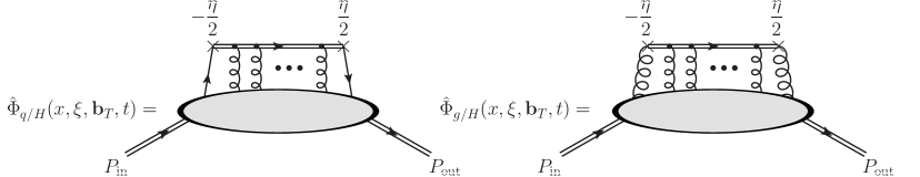
A graphical representation of the unsubtracted GTMD correlators defined in Eq. (LABEL:eq:GTMDdefinition) is given in Fig. 1. Here the double lines with an arbitrary number of gluons attaching to the hadronic blobs represent the (expansion of the) Wilson line. Notice that the actual Wilson line that connects the space-time points and runs back and forth along the light-cone direction defined by (future- or past-pointing, according to the process) and the two branches are connected along the transverse direction defined by at light-cone infinity. This latter connection is suppressed in Lorentz gauge and can thus be neglected.
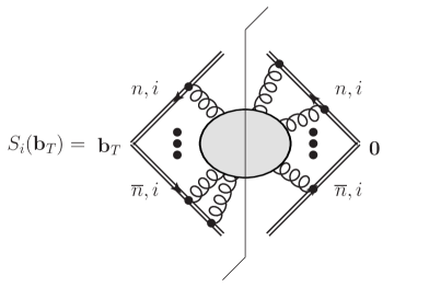
A graphical representation of the soft function defined in Eq. (3) is instead given in Fig. 2. Two pairs of longitudinal Wilson lines in and directions are joint at the origin and at the space-time point with transverse displacement . An arbitrary number of gluons is exchanged including loop corrections represented by the grey blob. Each gluon attachment to the Wilson lines comes with an SU(3) generator in the appropriate representation as indicated by the index associated to the Wilson lines.
2.2 Renormalisation and evolution of GTMDs
The subtracted GTMD correlator in Eq. (1), while being free of rapidity singularities, is UV divergent. In order to renormalise it, we need to separately renormalise the soft function and the unsubtracted GTMD correlator .
The soft function is renormalised multiplicatively as follows:
| (5) |
For completeness, in this expression we have explicitly reported all the possible dependences that emerge from a perturbative calculation. Specifically, we have: the scale and the regulator introduced by the regularisation of the rapidity divergences (to be discussed in Sect. 2.4), the scale and the dimensional regulator introduced by the regularisation of the UV divergences. Also notice the presence amongst the dependences of the renormalisation constant of the (squared) scale , usually dubbed rapidity scale, also discussed in Sect. 2.4.
The renormalisation of the unsubtracted GTMD correlators is also purely multiplicative, i.e. it does not imply any convolution nor mixing between quark and gluon operators:
| (6) |
This simple pattern is a direct consequence of the fact that the displacement prevents any contact divergence of the operators. Using Eqs. (5) and (6) in Eq. (1), one can easily deduce the renormalisation of the subtracted GTMD correlator:
| (7) |
Exploiting the fact that, in the limit , the bare subtracted GTMD correlator does not depend on either the renormalisation scale or on the rapidity scale , it is possible to derive the following evolution equations:
| (8) |
The anomalous dimensions and derive from the renormalisation constants as follows:
| (9) |
The first equation in Eq. (8) is usually referred to as Collins-Soper equation [66, 67], while the second is a more common renormalisation-group equation.
The anomalous dimensions in Eq. (9) can be mutually related by observing that the cross derivative of the GTMD correlator must coincide. Indeed, it turns out that:
| (10) |
where the anomalous dimension , usually called cusp anomalous dimension, only depends on the strong coupling . Therefore, it is a purely perturbative quantity that, for sufficiently large scales, admits the expansion:
| (11) |
Eq. (10) can be solved w.r.t. both and expressing these anomalous dimensions in terms of more fundamental quantities computable in perturbation theory. To do so, we need appropriate boundary conditions. For the boundary condition is conveniently set at the scale , with and the Euler constant, where it admits the perturbation expansion:
| (12) |
With this boundary condition, the solution to Eq. (10) reads:
| (13) |
We notice that, thanks to the integral in the r.h.s., this expression resums all powers in through its evolution, preventing the presence of potentially large logarithms. However, as we will explicitly see below, a perturbative calculation of at a generic fixed scale produces terms accompanied by powers of . Since is usually integrated over, these logarithms can become arbitrarily large invalidating any fixed-order calculation. Therefore, in phenomenological applications the resummed expression of in Eq. (13) is to be preferred over a fixed-order calculation.
We now solve Eq. (10) for . In this case, the boundary condition is conveniently set at where the anomalous dimension can be expanded as:
| (14) |
Owing to the fact that the r.h.s. of Eq. (10) does not depend of , the solution to the evolution equation is particularly simple and reads:
| (15) |
In conclusion, the evolution equations for the GTMD correlator take the explicit form:
| (16) |
where the relevant anomalous dimensions , , and are all perturbative quantities. As a by-product of the calculation of the matching functions presented below, we will extract the leading-term coefficients , , and . Unsurprisingly, they turn out to be identical to those obtained in TMD factorisation.
2.3 Matching on GPDs
As mentioned above, the transverse displacement is Fourier conjugated to the partonic transverse momentum . As a consequence, when , which corresponds to the emission of partons with large , it is legitimate to expect such emissions to be treatable in perturbation theory. As a matter of fact, in this regime hard emissions can be factorised into perturbatively calculable quantities, the matching functions, that allow one to express the GTMD correlators in terms of the corresponding collinear GPD correlators. The matching formula reads:
| (17) |
where , with , are the renormalised GPD correlators whose explicit definition can be found, e.g., in Ref. [57]. In addition, we have defined .
In order to extract the matching functions , we make use of the concept of parton-in-parton distribution [13] (sometimes also referred to as quark-target model, see e.g. Ref. [68]). The idea is to replace the hadronic states involved in the correlators in Eq. (LABEL:eq:GTMDdefinition) and in their collinear analogues with partonic states. Since the action of partonic fields on partonic states is computable in perturbation theory, this enables a direct calculation. It should be pointed out that the validity of this procedure is tightly connected to factorisation and the universality of the resulting partonic distributions [13]. Since so far, to the best of my knowledge, no actual factorisation theorems involving GTMDs have been proven,444However, factorisation is often assumed. See, for example, Refs. [53, 54, 55, 52]. here we simply assume its applicability. The parton-in-parton version of Eq. (17) is then:
| (18) |
where . Notice that we have dropped the dependence on that does not participate in a partonic computation. Now all quantities involved in the matching formula admit a perturbative expansion:
| (19) |
At the lowest order in , where no additional radiation is allowed, one finds that:
| (20) |
with and [57]. This immediately implies that:
| (21) |
These results allow us to determine the one-loop () correction to in terms of the one-loop GTMD and GPD parton-in-parton correlators:
| (22) |
Using the perturbative expansion of the renormalised soft function and unsubtracted parton-in-parton GTMD correlator :
| (23) |
with (see Eq. (44)) in Eq. (7), we obtain:
| (24) |
Notice that, while the single terms on r.h.s. of this equation depend on the rapidity regulator , the l.h.s. does not. This means that this dependence must cancel in this specific combination confirming at one loop the rapidity-divergence safety of the definition in Eq. (1). Plugging this identity into Eq. (22), finally gives:
| (25) |
Therefore, the computation of the one-loop corrections to the matching functions boils down to computing parton-in-parton unsubtracted GTMD and GPD correlators, and the soft function at the same order. Moreover, the computations of and of are closely related, with the latter recently presented in Ref. [57]. This similarity can be exploited to simplify the calculation. First of all, we notice that they are both made of a “real” and a “virtual” contribution:555Strictly speaking, since both GTMDs and GPDs are involved in exclusive processes, all contributions are virtual. However, one can distinguish between contributions that only affect either the left or the right part of the operator (i.e. that live at at or , with reference to Fig. 1), defined as virtual, and contributions that instead connect the two parts, defined as real. This is done in analogy with the inclusive case in which the final-state cut sets the real contributions on shell.
| (26) |
Since the virtual contribution to the GTMD correlator in space must, for kinematic reasons, be proportional to , its Fourier transform is independent from . But this is precisely the same kinematics used to compute the virtual contribution to the GPD correlator. Therefore, one finds:
| (27) |
such that:
| (28) |
To compute the difference in the r.h.s., we can again use the results of Ref. [57]. To do so, we observe that the only difference between and in space is that the integral in the latter is weighted by the phase , reflecting the displacement of the partonic fields. Specifically, one finds:
| (29) |
where is the real (and rapidity divergent) contribution to the one-loop GPD splitting functions, while the “residual” functions were so far unknown and are computed here for the first time (see Sect. 2.5). Importantly, the exponential in the integral in Eq. (29) regulates the UV divergence for [69]. As a consequence, the UV divergences of the GTMD correlator can only be in the virtual (diagonal) part, hence the simple renormalisation pattern in Eq. (6).
The integral in Eq. (29) can be computed analytically and evaluates to:
| (30) |
where . In the rightmost equality we have highlighted the fact that the pole for is of infrared origin. This divergence is cancelled in the difference in Eq. (28) by an analogous divergence in the UV-renormalised GPD correlator. To see this, we observe that the real part of the renormalised GPD correlator can be written as:
| (31) |
where:
| (32) |
From Eq. (31), it is apparent that the UV divergence has been removed leaving a , while the infrared divergence is still present. In addition, we also retained the next term in the expansion in powers of . This term, proportional to , multiplies a scaleless integral in which UV () and IR () poles cancel giving a vanishing result [70] that does not contribute to . However, since the IR contribution is cancelled by the GPD correlator, the UV pole does give a finite contribution in the combination in Eq. (28). Indeed, using Eqs. (29) and (31), Eq. (28) yields:
| (33) |
where the limit has already been taken using the equality:
| (34) |
Remarkably, all divergences have cancelled leaving a finite quantity. Plugging Eq. (33) into Eq. (25), we obtain:
| (35) |
It is now convenient to extract the rapidity divergence from in a way to facilitate the cancellation against the soft function . To this purpose, we now introduce the particular strategy that will be used to regulate the rapidity divergences. We will employ the principal-value prescription [63] that acts on eikonal propagators of the kind and by replacing them with their principal-valued version, that is:
| (36) |
with , and analogously for with replaced by . The momenta and are to be thought as the light-like momenta () of two highly energetic projectiles that collide with large centre-of-mass energy . is precisely the scale first introduced in Eq. (5) as a consequence of the regularisation of rapidity divergences and that will appear explicitly only in the soft function. When integrating over the partonic momentum , the longitudinal projection is usually parameterised as , with the variable running in the interval . One can then show that the principal-value prescription is equivalent to replacing:
| (37) |
where the -prescription is defined as:
| (38) |
for a test function well-behaved at .
With this at hand, we can replace in Eq. (35) with the full splitting function using the following equality:
| (39) |
In the second line we have used the explicit form of the virtual contribution to the splitting function extracted from Ref. [57]. The color factors are defined as:
| (40) |
and the values of the coefficient are:
| (41) |
with and the number of active quark flavours. Finally, in the third line of Eq. (39) we have used Eq. (37) to regularise the divergent integral in . We can now plug Eq. (39) into Eq. (35) to obtain:
| (42) |
Since the splitting functions have been computed in Ref. [57], all we are left with to obtain the one-loop correction to the matching functions is to compute the soft function and the residual functions . This will be done next in Sects. 2.4 and 2.5, respectively.
2.4 The soft function
Many calculations of the soft function to one-loop order and beyond exist in the literature. For example, one-loop results can be found in Refs. [58, 71, 72, 73, 61, 74]. As of today, also two-loop [75, 72, 73] and three-loop [76, 77] results have been presented. As mentioned above, the soft function is affected by rapidity divergences. They are caused by the presence of eikonal propagators like and cannot be regulated by means of dimensional regularisation. Therefore, an additional regulator needs to be introduced. We will use the principal-value prescription [63] introduced in the previous section that, to the best of my knowledge, is used here for the first time to compute the soft function. The soft function is also affected by UV divergences that we regularise by means of dimensional regularisation.
The ultimate goal of this section is to compute the first two terms, , of the series in Eq. (23) for the renormalised soft function. To do so, we start from the perturbative series of the bare soft function:
| (43) |
The leading-order, , is trivial. To compute it, we simply approximate all the Wilson lines in Eq. (3) with the unity operator in the appropriate colour-group representation. This immediately gives:
| (44) |
We now move on to computing the one-loop correction, i.e. the term in the series in Eq. (43). One-loop diagrams in which the gluon attaches to Wilson lines pointing in the same light-cone direction are proportional to either or , and thus give no contribution. On the contrary, the diagrams displayed in Fig. 3 have a gluon that attaches to Wilson lines pointing in different directions. Therefore, they are proportional to , giving a non-null contribution.
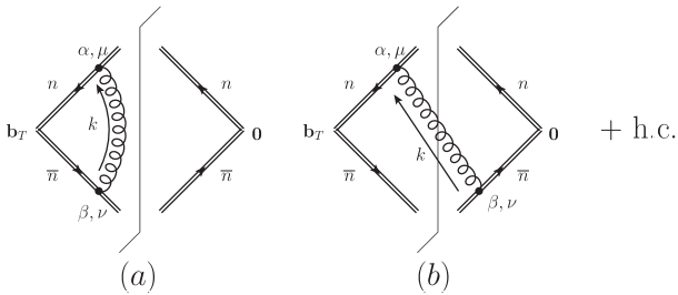
Applying standard Feynman rules in Lorentz gauge [13] and using the principal-value prescription to regulate the eikonal propagators, diagrams (a) and (b) along with their respective hermitian conjugates separately evaluate to:
| (45) |
The net result for the one-loop correction to the bare soft function is:
This result agrees with that of Ref. [72] despite the different (but closely related) regularisation of the rapidity divergences.
A couple of additional comments are in order. First, from the second line of Eq. (2.4) we immediately see that . This reflects the fact that the soft function must unitarise for . Considering the leading-order result in Eq. (44), this requirement is indeed fulfilled to one-loop accuracy by our calculation. It is also interesting to observe that is UV finite:
| (47) |
This was to be expected because the transverse displacement regulates the UV divergence in real diagrams. This is a further consistency check of the calculation.
We can now renormalise the soft function. This is done multiplicatively as in Eq. (5). Considering the first two orders of the bare soft function, Eqs. (44) and (2.4), the renormalisation constant in the scheme reads:666Notice that in the scheme poles in , rather than in , are subtracted. The expansion in the second line of Eq. (2.4) is purposely written in terms of in view of renormalisation in the scheme.
| (48) |
Here, the arbitrary rapidity scale is introduced as a proxy to parameterise finite contributions. Using this renormalisation constant, one obtains the first two coefficients of the perturbative expansion of the renormalised soft function:
| (49) |
Evidently, is still affected by a rapidity divergence for . This divergence is precisely what is needed to cancel an analogous divergence of the unsubtracted GTMD correlator. Indeed, plugging into Eq. (42), one finds:
where the rapidity divergence has cancelled, leaving an explicitly finite result. We now just need to compute the residual functions to complete the picture.
2.5 The unsubtracted GTMD correlators
In this section, we present the results for the one-loop unsubtracted parton-in-parton GTMD correlators as defined in Eq. (LABEL:eq:GTMDdefinition). This calculation is functional to the extraction of the residual functions as well as of the renormalisation constant in Eq. (6).
Practically speaking, the computation is closely related to that of the splitting functions presented in Ref. [57]. As already discussed in Sect. 2.3, the real contribution to the unsubtracted parton-in-parton GTMD is a simple generalisation of the real contribution to the respective GPD (see Eq. (29)). In addition, as again discussed in Sect. 2.3, the virtual contribution coincides with . The only new element w.r.t. Ref. [57] is that we need to retain, not only the pole part of the correlator, but also the first finite correction in the expansion in powers of . This is precisely where the residual functions reside.
The main difference between the theoretical setup of this work and that of Ref. [57] is the choice of the gauge. While here we opted for the Lorentz gauge, in Ref. [57] the light-cone gauge was used. However, a simple analysis shows that this difference is immaterial, at least at one-loop accuracy. The reasoning runs as follows. The GPD correlators are by construction gauge invariant, signifying that the light-cone-gauge result of Ref. [57] must coincide with a calculation in Lorenz gauge.777I have explicitly verified this statement in the channel by re-performing the calculation of Ref. [57] in Lorentz gauge. Now, the differences between the GPD and the GTMD correlators are:
-
1.
a transverse displacement of the operator that causes the appearance of a phase in the real diagrams (see Sect. 2.3),
-
2.
the appearance of a transverse Wilson line at light-cone infinity.
We have already discussed in Sect. 2.3 how to take care of the phase while, in Lorentz gauge, the transverse Wilson line gives no contribution. The conclusion is that, at least at one loop, the light-cone-gauge calculation of the GPD correlators can be entirely “recycled” to obtain the GTMD correlators in Lorentz gauge. Based on this conclusion, we refer the reader to Ref. [57] for the details of the calculation. Here, we only report the result for the bare unsubtracted GTMD correlators:
where we have labelled the poles as IR or UV. Using the leading-order result:
| (52) |
that descend from Eq. (20), we can extract the renormalisation constant as defined in Eq. (6) up to one loop:
| (53) |
The residual functions in Eq. (LABEL:eq:BareUnsubGTMD) are best given for non-singlet and singlet GTMD combinations, respectively defined as:
| (54) |
The sums run over the active quark flavours and the anti-quark correlators are defined as:
| (55) |
In addition, it is convenient to introduce the following decomposition:
| (56) |
In the non-singlet sector one finds:
| (57) |
while the singlet results are:
| (58) |
All the expressions for and above are singular at . It turns out that this singularity cancels out in the combination in Eq. (56) for , , and . Unfortunately this does not happen for and . Specifically, for and , one is left with undefined integrals of this kind:
| (59) |
Nevertheless, appropriately interpreting these integrals as principal-values, one can use a trick presented in Ref. [57] to obtain a numerically amenable representation that reads:
| (60) |
However, these integrals are clearly divergent for because in this limit the pole of the integrand becomes an end-point singularity. As a consequence, as we will explicitly see in Sect. 3, the GTMD correlator will manifest a divergent behaviour around . We also notice that these divergences, being limited to and , emerge from the convolution of the matching functions with the gluon GPDs. Therefore, one may argue that vanishing gluon GPDs at would guarantee the finiteness of the GTMD correlator at . However, this constraint on the gluon GPDs seems to be hard to fulfil in full generality in that it should hold at all scales.
In this respect, I can foresee two possible scenarios. In the first scenario, the gluon GPDs obey a specific functional constraint such that they remain null at at all scales. Incidentally, this constraint seems to be possible to realise by means of the so-called “shadow” GPDs recently introduced in Ref. [78]. In the second scenario, the gluon GPDs are different from zero at causing the GTMD correlator to diverge in this point. To the best of my knowledge, while even a discontinuity at at the level of GPDs would cause the breaking of leading-twist collinear factorisation in deeply-virtual Compton scattering (DVCS) [79], a divergent GTMD correlator at is not in principle forbidden. It is interesting to observe that, beyond leading twist, discontinuities at in DVCS partonic amplitudes do appear even in the collinear case, see e.g. Ref. [80, 81, 82]. However, in those papers it has been shown that these discontinuities are such that they do not break factorisation within the relevant accuracy.888I thank B. Pasquini for having drawn my attention to these works.
As discussed in Ref. [83] in the context of DVCS, it can also be argued that the singularity at is a consequence of a kinematic enhancement due to the emission of soft-collinear gluons that spoil the perturbative convergence in this region. Analogously to the case of soft gluons in the threshold region in deep-inelastic scattering [84, 85], their emission can be resummed to all orders in the strong coupling producing better-behaved results around [83].999I am grateful to C. Mezrag for pointing me to Ref. [83]. In any event, this point deserves further investigations.
2.6 Forward limit of the matching functions
To the best of my knowledge, this is the first calculation of GTMD matching functions to one-loop accuracy ever performed. As such, there are no previous calculations that can be used to compare these results to. However, these matching functions need to tend to their well-known forward counterpart used to match TMDs onto collinear PDFs.
To perform this check, we first observe that the structure of Eq. (LABEL:eq:finalres2) is the same as that found in the TMD case: see for instance Eq. (4.8) of Ref. [58]. The forward limit is realised by taking the limit that is equivalent to . In this limit, we have already verified in Ref. [57] that the GPD splitting functions tend to the Altarelli-Parisi splitting functions. We can therefore safely simplify Eq. (LABEL:eq:finalres2) by setting in such a way that all logarithms vanish. Expressing the matching functions in the basis defined in Eq. (54), we find:
| (61) |
When taking the limit , the term proportional to in the decomposition of in Eq. (56) drops. This leaves only the term proportional to that, introduced in the convolution integral as defined in Eq. (17), turns it into a standard Mellin convolution. Therefore, all we need to do is to take the limit of the functions . This is easily done using Eqs. (57) and (58) and the result is:
| (62) |
that indeed coincide with the TMD results (see, e.g., Ref. [60]).
2.7 Anomalous dimensions
As discussed in Sect. 2.2, the knowledge of the renormalisation constants of soft function and unsubtracted GTMD correlators allows us to extract the anomalous dimensions that govern the evolution of the normalised GTMD correlators (see Eq. (8)). Using Eq. (9) with the normalisation constants and respectively given in Eqs. (48) and (53), such that:
| (63) |
one immediately finds:
| (64) |
Notice that, for computing the total derivative of w.r.t. as prescribed by the second equation in Eq. (9), we have used the identity:
| (65) |
where is the four-dimensional QCD -function that governs the running of the strong coupling:
| (66) |
The cusp anomalous dimension is extracted using Eq. (10) and equals:101010Notice that deriving either w.r.t. or w.r.t. consistently gives the same result.
| (67) |
Finally, Eqs. (64) and (67) allow us to extract the leading-order coefficients:
| (68) |
These results coincide with those obtained in the TMD framework (see, e.g., Ref. [86] and references therein for a recent overview). It is therefore legitimate to expect that the same holds true to all orders such that we can use the known higher-order corrections to these quantities to evolve GTMDs to higher accuracies. We will do so in the next section.
3 Numerical setup
In this section, we present numerical results showing how the matching functions computed above can be used to reconstruct realistic GTMDs by combining: a sensible model for GPDs along with collinear off-forward evolution, perturbative TMD evolution, and a model for the non-perturbative transverse effects as determined by recent TMD extractions.
The limitation of this procedure is that it can only be applied to GTMDs that have, at the same time, a projection on a GPD and on a TMD.111111By projection of a GTMD on a GPD, it is meant the integral of the former over the partonic transverse momentum or, alternatively (and perhaps more correctly), the GPD on which the GTMD matches at large . While the projection of a GTMD on a TMD is its forward limit, . It is well-known that several GTMDs do not have projections either on GPDs or on TMDs, in the sense that their contribution to the correlator vanishes by kinematics [35, 38]. This largely restricts the range of possibilities. In addition, to give an estimate of such GTMDs, it is highly desirable that the GPDs and TMDs on which they project are, to some extent, phenomenologically known.
Using the results of Refs. [35, 38], the renormalised GTMD correlator, Eq. (7), has the following tensorial decomposition:
| (69) |
with and being respectively the spinors of the incoming and outgoing hadron having mass , and where we have used the shorthand notation . The scalar coefficients , with , are the actual GTMD distributions (GTMDs for short). Each of them can be split into a T-even and a T-odd part, both real, as follows:
| (70) |
The peculiarity of is that it conserves (flips) the sign upon swapping of the Wilson line from past to future pointing and viceversa.
The one GTMD that fulfils all the requirements stated above is . As a matter of fact, in space and at small , matches on the following combination of GPDs:
| (71) |
where we have replaced with everywhere because does not depend of the direction on . Currently, different models for and exist. In addition, the forward limit of is the fully unpolarised TMD , that is:
| (72) |
Accurate phenomenological determinations from data of , with , have recently been presented.
In order to compute numerically, we employ a standard procedure used in TMD factorisation (see, e.g., Ref. [15]). Let us first state the complete formula and then comment on it:
First, we have introduced the so-called -prescription with this particular functional form [14, 15, 17]:
| (74) |
and the associated scale . The scale is usually identified with the physical hard scale of the process under consideration. In all cases, one must have . Since the -space GTMD is obtained through a Fourier transform of the -space expression, the scope of the -prescription is to prevent the scale from becoming too low such to enter the non-perturbative regime when . Indeed, if became of the order of or smaller, any perturbative calculation would be invalidated. To this purpose, Eq. (74) is engineered in a way that:
| (75) |
In addition, Eq. (74) is also such that:
| (76) |
This last property is not strictly needed but it helps keep under better control the large- region [87, 88].
While the -prescription ensures the applicability of perturbation theory, it remains necessary to keep into account non-perturbative transverse effects. This is done through the function in the third line of Eq. (3) that parameterises non-perturbative large- effects. See Refs. [15, 16, 17] for recent global determinations of from experimental data in the TMD framework. For our numerical estimates, we will use the determination of from Ref. [15], henceforth referred to as PV19 (for Pavia 2019), for both quark and gluon distributions.121212Notice that the extracted in Ref. [15] strictly applies to quark distributions. Since, to the best of my knowledge, there is no comparably reliable analogue for the gluon, we will use the same also for this distribution. in Eq. (3) only depends on , , and the combination (the latter related to the evolution pattern). However, in the GTMD case this function should in principle also depend on and . Since from PV19 is obtained from a fit of TMDs where and are identically zero, we do not have access to the non-perturbative transverse dependence on these variables. Nonetheless, this dependence is expected to be mild in that most of the effect is accounted for by the collinear GPDs.131313The argument behind this statement is the fact that is effectively obtained as a ratio of GTMDs computed a different values of , see for example Ref. [15] for a discussion in the TMD framework. As a consequence, any dependence on kinematic variables is expected to be relatively mild. This turns out to be the case for the longitudinal momentum fraction [15].
The first line of Eq. (3) corresponds to the matching onto the collinear GPDs as in Eq. (71). However, the scales at which the matching is performed are chosen to be so that the matching functions are free of potentially large logarithms. The GPDs and are computed using the Goloskokov-Kroll (GK) model [89, 90, 91] at the initial scale GeV and appropriately evolved to through collinear evolution.
The evolution to the hard scales and is provided by the factor in the second line of Eq. (3), often referred to as Sudakov form factor. This factor results from the solution of the evolution equations in Eq. (16) and reads:
| (77) |
As discussed in Sect. 2.2, the anomalous dimension , , and are computable in perturbation theory and they (are expected to) coincide with their TMD counterparts.
Finally, we can obtain the in space by taking a 2D Fourier transform of Eq. (3) w.r.t. that, with abuse of notation, gives:
| (78) |
where is a Bessel function of the first kind.
The theoretical precision of the formula in Eq. (3) is usually expressed in terms of logarithmic accuracy. Tab. 1 of Ref. [15] tells us that the knowledge of the matching functions up to would in principle allow us to reach next-to-next-to-leading logarithmic (NNLL) accuracy. In the case of GTMDs, the only obstacle to reaching this accuracy is the evolution of collinear GPDs that, as of today, is publicly available only up to leading order [57]. However, in the following we will use a NNLL-accurate setup, except for the GPD evolution for which the (i.e. leading-order) splitting functions are used. This practically means that and are computed at , at , at , and the evolution of the strong coupling is computed using a function truncated at . In the following, in order to simplify the presentation, we will set .
The numerical implementation of the GTMD in Eq. (3) and its Fourier transform Eq. (78) makes use of a compound of publicly available tools. Specifically, the GK model for the GPDs and at the initial scale is provided by PARTONS [92]141414https://partons.cea.fr/partons/doc/html/index.html; their collinear evolution as well as the perturbative ingredients relevant to the matching and the Sudakov form factor are provided by APFEL++ [93, 94]151515https://github.com/vbertone/apfelxx; the non-perturbative function and the Fourier transform are instead provided by NangaParbat [15]161616https://github.com/MapCollaboration/NangaParbat. The resulting code is public171717https://github.com/vbertone/GTMDMatchingFunctions and can be used to reproduce the results shown below.
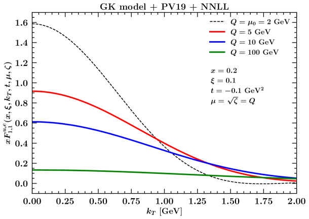
We can finally present a selection of quantitative results. We start with Fig. 4 that shows the behaviour w.r.t. of the up-quark GTMD at fixed values of , , and for different values of the hard scale . The curve at the GPD initial scale is also shown. The typical broadening of the distribution caused by the Sudakov form factor as increases is clearly observed [95, 56]. We also note that the curve at becomes negative at large as a consequence of the specific functional form used here. The gluon distribution behaves very similarly, therefore we do not show the corresponding plot.

It is also interesting to look at how the dependence of changes with . To this purpose, Fig. 5 shows curves for the up-quark distribution at fixed values of , , and for different values of . The black dashed line corresponds to that is, up to a fully non-perturbative dependence of the underlying GPDs, the “partonic” forward limit. The behaviour in is clearly non monotonic but exhibits a strong suppression as the value of approaches one. Again, the gluon distribution does not present any further salient features and thus is not shown.
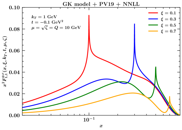
Finally, we consider the behaviour of as a function of the longitudinal momentum fraction . As pointed out in Sect. 2.5, and cause a divergence at in both quark and gluon GTMD correlators. To study this effect, we concentrate on the gluon GTMD and in Fig. 6 we show this distribution (weighted by to improve the readability of the plot) as a function of at fixed values of , , and for different values of . It is evident that indeed the curves exhibit a divergence at that is a manifestation of the divergence of the principal-valued integral in Eq. (60) for . The conclusion is that GTMDs obtained through perturbative matching onto GPDs beyond tree level are undefined at . Whether this is an acceptable feature of GTMDs remains an open question. As already mentioned in Sect. 2.5, a possibility to remove the divergence is to require the gluon GPDs to vanish at at all scales.
4 Conclusions
The main result of this paper is the calculation of the complete set of one-loop unpolarised GTMD matching functions. These perturbative functions allow one to express GTMDs at large partonic transverse momentum (or equivalently at low ) in terms of GPDs. They are obtained employing a rapidity-divergence-free definition of the GTMD correlator [56] that combines the soft function with the unsubtracted GTMD correlator. In order to carry out the calculation, the principal-value regulator for rapidity divergences has been used, allowing us to obtain one-loop results for soft function, confirming previous results, and unsubtracted GTMD correlator, that are instead original. By renormalising the UV divergences of these objects, we have also extracted the one-loop anomalous dimensions, again confirming known results. In addition, as a consistency check, we have verified that in the limit the one-loop GTMD matching functions thus obtained reproduce the well-know TMD results.
In the last part of the paper, we have presented a quantitative study by implementing the matching functions and combining them with other perturbative and non-perturbative ingredients necessary to fully reconstruct the GTMDs , with , at NNLL accuracy. We have studied their dependence along with the scale evolution and the dependence on the skewness . An interesting consequence of our calculation is that, beyond tree level, GTMD matching functions yield GTMDs that exhibit a pole at . The origin of this singularity is unclear and may signal the need of additional theoretical constraints on the underlying gluon GPDs. A more extensive investigation on this point is left for a future study. Finally, we stress that the numerical results presented here are readily accessible in that all of the relevant ingredients are available in public codes. A code that consistently combines them to reproduce the plots of this paper is also released with the paper.
The calculation presented here is limited to the unpolarised twist-2 Lorentz structure (see Eq. (LABEL:eq:GTMDdefinition)). The extension of this study to the remaining twist-2 structures is planned for the future. This will require computing the corresponding splitting functions along the lines of Ref. [57] as well as the one-loop corrections to the unsubtracted GTMD correlators. Phenomenological applications of the GTMDs presented here are also envisaged. Specifically, the computation of measurable (and possible measured) cross sections using the GTMDs presented in this paper would allow us to gauge the accuracy of the calculation as well as the reliability of the underlying non-perturbative ingredients, such as the GPDs and the TMDs.
Acknowledgements
I acknowledge stimulating discussions with S. Bhattacharya, H. Dutrieux, M. G. Echevarria, and H. Moutarde. I am particularly grateful to C. Mezrag B. Pasquini, and S. Rodini for a critical reading of the manuscript. This work was supported by the European Union’s Horizon 2020 research and innovation programme under grant agreement STRONG 2020 - No 824093.
References
- [1] R. D. Ball et al., “The PDF4LHC21 combination of global PDF fits for the LHC Run III,” J. Phys. G, vol. 49, no. 8, p. 080501, 2022.
- [2] T.-J. Hou et al., “New CTEQ global analysis of quantum chromodynamics with high-precision data from the LHC,” Phys. Rev. D, vol. 103, no. 1, p. 014013, 2021.
- [3] S. Bailey, T. Cridge, L. A. Harland-Lang, A. D. Martin, and R. S. Thorne, “Parton distributions from LHC, HERA, Tevatron and fixed target data: MSHT20 PDFs,” Eur. Phys. J. C, vol. 81, no. 4, p. 341, 2021.
- [4] R. D. Ball et al., “The path to proton structure at 1% accuracy,” Eur. Phys. J. C, vol. 82, no. 5, p. 428, 2022.
- [5] J. McGowan, T. Cridge, L. A. Harland-Lang, and R. S. Thorne, “Approximate N3LO Parton Distribution Functions with Theoretical Uncertainties: MSHT20aN3LO PDFs,” 7 2022.
- [6] N. Sato, C. Andres, J. J. Ethier, and W. Melnitchouk, “Strange quark suppression from a simultaneous Monte Carlo analysis of parton distributions and fragmentation functions,” Phys. Rev. D, vol. 101, no. 7, p. 074020, 2020.
- [7] H. Abdolmaleki, M. Soleymaninia, H. Khanpour, S. Amoroso, F. Giuli, A. Glazov, A. Luszczak, F. Olness, and O. Zenaiev, “QCD analysis of pion fragmentation functions in the xFitter framework,” Phys. Rev. D, vol. 104, no. 5, p. 056019, 2021.
- [8] E. Moffat, W. Melnitchouk, T. C. Rogers, and N. Sato, “Simultaneous Monte Carlo analysis of parton densities and fragmentation functions,” Phys. Rev. D, vol. 104, no. 1, p. 016015, 2021.
- [9] R. A. Khalek, V. Bertone, and E. R. Nocera, “Determination of unpolarized pion fragmentation functions using semi-inclusive deep-inelastic-scattering data,” Phys. Rev. D, vol. 104, no. 3, p. 034007, 2021.
- [10] I. Borsa, D. de Florian, R. Sassot, M. Stratmann, and W. Vogelsang, “Towards a Global QCD Analysis of Fragmentation Functions at Next-to-Next-to-Leading Order Accuracy,” Phys. Rev. Lett., vol. 129, no. 1, p. 012002, 2022.
- [11] R. A. Khalek, V. Bertone, A. Khoudli, and E. R. Nocera, “Pion and kaon fragmentation functions at next-to-next-to-leading order,” 4 2022.
- [12] J. C. Collins, D. E. Soper, and G. F. Sterman, “Transverse Momentum Distribution in Drell-Yan Pair and W and Z Boson Production,” Nucl. Phys. B, vol. 250, pp. 199–224, 1985.
- [13] J. Collins, Foundations of perturbative QCD, vol. 32. Cambridge University Press, 11 2013.
- [14] A. Bacchetta, F. Delcarro, C. Pisano, M. Radici, and A. Signori, “Extraction of partonic transverse momentum distributions from semi-inclusive deep-inelastic scattering, Drell-Yan and Z-boson production,” JHEP, vol. 06, p. 081, 2017. [Erratum: JHEP 06, 051 (2019)].
- [15] A. Bacchetta, V. Bertone, C. Bissolotti, G. Bozzi, F. Delcarro, F. Piacenza, and M. Radici, “Transverse-momentum-dependent parton distributions up to N3LL from Drell-Yan data,” JHEP, vol. 07, p. 117, 2020.
- [16] I. Scimemi and A. Vladimirov, “Non-perturbative structure of semi-inclusive deep-inelastic and Drell-Yan scattering at small transverse momentum,” JHEP, vol. 06, p. 137, 2020.
- [17] A. Bacchetta, V. Bertone, C. Bissolotti, G. Bozzi, M. Cerutti, F. Piacenza, M. Radici, and A. Signori, “Unpolarized Transverse Momentum Distributions from a global fit of Drell-Yan and Semi-Inclusive Deep-Inelastic Scattering data,” 6 2022.
- [18] M. Boglione, J. O. Gonzalez-Hernandez, and A. Simonelli, “Transverse Momentum Dependent Fragmentation Functions from recent BELLE data,” 6 2022.
- [19] M. A. Ebert, J. K. L. Michel, I. W. Stewart, and Z. Sun, “Disentangling Long and Short Distances in Momentum-Space TMDs,” 1 2022.
- [20] X.-D. Ji, “Off forward parton distributions,” J. Phys. G, vol. 24, pp. 1181–1205, 1998.
- [21] M. V. Polyakov, “Generalized parton distributions and strong forces inside nucleons and nuclei,” Phys. Lett. B, vol. 555, pp. 57–62, 2003.
- [22] M. Burkardt, “Impact parameter space interpretation for generalized parton distributions,” Int. J. Mod. Phys. A, vol. 18, pp. 173–208, 2003.
- [23] M. Diehl, “Generalized parton distributions in impact parameter space,” Eur. Phys. J. C, vol. 25, pp. 223–232, 2002. [Erratum: Eur.Phys.J.C 31, 277–278 (2003)].
- [24] X.-D. Ji, “Gauge-Invariant Decomposition of Nucleon Spin,” Phys. Rev. Lett., vol. 78, pp. 610–613, 1997.
- [25] K. Kumerički and D. Müller, “Description and interpretation of DVCS measurements,” EPJ Web Conf., vol. 112, p. 01012, 2016.
- [26] H. Dutrieux, H. Dutrieux, O. Grocholski, O. Grocholski, H. Moutarde, H. Moutarde, P. Sznajder, and P. Sznajder, “Artificial neural network modelling of generalised parton distributions,” Eur. Phys. J. C, vol. 82, no. 3, p. 252, 2022. [Erratum: Eur.Phys.J.C 82, 389 (2022)].
- [27] Y. Guo, X. Ji, and K. Shiells, “Generalized parton distributions through universal moment parameterization: zero skewness case,” 7 2022.
- [28] D. P. Anderle et al., “Electron-ion collider in China,” Front. Phys. (Beijing), vol. 16, no. 6, p. 64701, 2021.
- [29] R. Abdul Khalek et al., “Science Requirements and Detector Concepts for the Electron-Ion Collider: EIC Yellow Report,” 3 2021.
- [30] X. Ji, “Parton Physics on a Euclidean Lattice,” Phys. Rev. Lett., vol. 110, p. 262002, 2013.
- [31] A. V. Radyushkin, “Quasi-parton distribution functions, momentum distributions, and pseudo-parton distribution functions,” Phys. Rev. D, vol. 96, no. 3, p. 034025, 2017.
- [32] A. V. Belitsky, X.-d. Ji, and F. Yuan, “Quark imaging in the proton via quantum phase space distributions,” Phys. Rev. D, vol. 69, p. 074014, 2004.
- [33] X.-d. Ji, “Viewing the proton through ’color’ filters,” Phys. Rev. Lett., vol. 91, p. 062001, 2003.
- [34] S. Meissner, A. Metz, M. Schlegel, and K. Goeke, “Generalized parton correlation functions for a spin-0 hadron,” JHEP, vol. 08, p. 038, 2008.
- [35] S. Meissner, A. Metz, and M. Schlegel, “Generalized parton correlation functions for a spin-1/2 hadron,” JHEP, vol. 08, p. 056, 2009.
- [36] C. Lorce and B. Pasquini, “Quark Wigner Distributions and Orbital Angular Momentum,” Phys. Rev. D, vol. 84, p. 014015, 2011.
- [37] C. Lorce, B. Pasquini, X. Xiong, and F. Yuan, “The quark orbital angular momentum from Wigner distributions and light-cone wave functions,” Phys. Rev. D, vol. 85, p. 114006, 2012.
- [38] C. Lorcé and B. Pasquini, “Structure analysis of the generalized correlator of quark and gluon for a spin-1/2 target,” JHEP, vol. 09, p. 138, 2013.
- [39] C. Lorce, B. Pasquini, and M. Vanderhaeghen, “Unified framework for generalized and transverse-momentum dependent parton distributions within a 3Q light-cone picture of the nucleon,” JHEP, vol. 05, p. 041, 2011.
- [40] K. Kanazawa, C. Lorcé, A. Metz, B. Pasquini, and M. Schlegel, “Twist-2 generalized transverse-momentum dependent parton distributions and the spin/orbital structure of the nucleon,” Phys. Rev. D, vol. 90, no. 1, p. 014028, 2014.
- [41] C. Lorcé and B. Pasquini, “Multipole decomposition of the nucleon transverse phase space,” Phys. Rev. D, vol. 93, no. 3, p. 034040, 2016.
- [42] Y. Hagiwara, Y. Hatta, and T. Ueda, “Wigner, Husimi, and generalized transverse momentum dependent distributions in the color glass condensate,” Phys. Rev. D, vol. 94, no. 9, p. 094036, 2016.
- [43] Y. Hagiwara, Y. Hatta, R. Pasechnik, M. Tasevsky, and O. Teryaev, “Accessing the gluon Wigner distribution in ultraperipheral collisions,” Phys. Rev. D, vol. 96, no. 3, p. 034009, 2017.
- [44] J. More, A. Mukherjee, and S. Nair, “Quark Wigner Distributions Using Light-Front Wave Functions,” Phys. Rev. D, vol. 95, no. 7, p. 074039, 2017.
- [45] J. More, A. Mukherjee, and S. Nair, “Wigner Distributions For Gluons,” Eur. Phys. J. C, vol. 78, no. 5, p. 389, 2018.
- [46] S. Bhattacharya, C. Cocuzza, and A. Metz, “Generalized quasi parton distributions in a diquark spectator model,” Phys. Lett. B, vol. 788, pp. 453–463, 2019.
- [47] H. Mäntysaari, N. Mueller, and B. Schenke, “Diffractive Dijet Production and Wigner Distributions from the Color Glass Condensate,” Phys. Rev. D, vol. 99, no. 7, p. 074004, 2019.
- [48] N. Kaur and H. Dahiya, “Quark Wigner Distributions and GTMDs of Pion in the Light-Front Holographic Model,” Eur. Phys. J. A, vol. 56, no. 6, p. 172, 2020.
- [49] F. Salazar and B. Schenke, “Diffractive dijet production in impact parameter dependent saturation models,” Phys. Rev. D, vol. 100, no. 3, p. 034007, 2019.
- [50] X. Luo and H. Sun, “T-odd generalized and quasi transverse momentum dependent parton distribution in a scalar spectator model,” Eur. Phys. J. C, vol. 80, no. 9, p. 828, 2020.
- [51] J.-L. Zhang, Z.-F. Cui, J. Ping, and C. D. Roberts, “Contact interaction analysis of pion GTMDs,” Eur. Phys. J. C, vol. 81, no. 1, p. 6, 2021.
- [52] D. Boer and C. Setyadi, “GTMD model predictions for diffractive dijet production at EIC,” Phys. Rev. D, vol. 104, no. 7, p. 074006, 2021.
- [53] Y. Hatta, B.-W. Xiao, and F. Yuan, “Probing the Small- x Gluon Tomography in Correlated Hard Diffractive Dijet Production in Deep Inelastic Scattering,” Phys. Rev. Lett., vol. 116, no. 20, p. 202301, 2016.
- [54] S. Bhattacharya, A. Metz, and J. Zhou, “Generalized TMDs and the exclusive double Drell–Yan process,” Phys. Lett. B, vol. 771, pp. 396–400, 2017. [Erratum: Phys.Lett.B 810, 135866 (2020)].
- [55] S. Bhattacharya, A. Metz, V. K. Ojha, J.-Y. Tsai, and J. Zhou, “Exclusive double quarkonium production and generalized TMDs of gluons,” 2 2018.
- [56] M. G. Echevarria, A. Idilbi, K. Kanazawa, C. Lorcé, A. Metz, B. Pasquini, and M. Schlegel, “Proper definition and evolution of generalized transverse momentum dependent distributions,” Phys. Lett. B, vol. 759, pp. 336–341, 2016.
- [57] V. Bertone, H. Dutrieux, C. Mezrag, J. M. Morgado, and H. Moutarde, “Revisiting evolution equations for generalised parton distributions,” 6 2022.
- [58] M. G. Echevarria, A. Idilbi, and I. Scimemi, “Factorization Theorem For Drell-Yan At Low And Transverse Momentum Distributions On-The-Light-Cone,” JHEP, vol. 07, p. 002, 2012.
- [59] J. C. Collins, “What exactly is a parton density?,” Acta Phys. Polon. B, vol. 34, p. 3103, 2003.
- [60] M. G. Echevarria, I. Scimemi, and A. Vladimirov, “Unpolarized Transverse Momentum Dependent Parton Distribution and Fragmentation Functions at next-to-next-to-leading order,” JHEP, vol. 09, p. 004, 2016.
- [61] M. A. Ebert, I. W. Stewart, and Y. Zhao, “Towards Quasi-Transverse Momentum Dependent PDFs Computable on the Lattice,” JHEP, vol. 09, p. 037, 2019.
- [62] A. Idilbi and I. Scimemi, “Singular and Regular Gauges in Soft Collinear Effective Theory: The Introduction of the New Wilson Line T,” Phys. Lett. B, vol. 695, pp. 463–468, 2011.
- [63] G. Curci, W. Furmanski, and R. Petronzio, “Evolution of Parton Densities Beyond Leading Order: The Nonsinglet Case,” Nucl. Phys. B, vol. 175, pp. 27–92, 1980.
- [64] X.-d. Ji and F. Yuan, “Parton distributions in light cone gauge: Where are the final state interactions?,” Phys. Lett. B, vol. 543, pp. 66–72, 2002.
- [65] S. Rodini, Proton structure, an iridescent study: from parton distributions to the emergence of the proton mass. PhD thesis, Universita’ Di Pavia, Pavia U., 2021.
- [66] J. C. Collins and D. E. Soper, “Back-To-Back Jets in QCD,” Nucl. Phys. B, vol. 193, p. 381, 1981. [Erratum: Nucl.Phys.B 213, 545 (1983)].
- [67] J. C. Collins and D. E. Soper, “Back-To-Back Jets: Fourier Transform from B to K-Transverse,” Nucl. Phys. B, vol. 197, pp. 446–476, 1982.
- [68] K. Goeke, S. Meissner, A. Metz, and M. Schlegel, “Checking the Burkardt sum rule for the Sivers function by model calculations,” Phys. Lett. B, vol. 637, pp. 241–244, 2006.
- [69] A. Bacchetta, D. Boer, M. Diehl, and P. J. Mulders, “Matches and mismatches in the descriptions of semi-inclusive processes at low and high transverse momentum,” JHEP, vol. 08, p. 023, 2008.
- [70] J. C. Collins, Renormalization: An Introduction to Renormalization, The Renormalization Group, and the Operator Product Expansion, vol. 26 of Cambridge Monographs on Mathematical Physics. Cambridge: Cambridge University Press, 1986.
- [71] A. A. Vladimirov, “TMD PDFs in the Laguerre polynomial basis,” JHEP, vol. 08, p. 089, 2014.
- [72] M. G. Echevarria, I. Scimemi, and A. Vladimirov, “Universal transverse momentum dependent soft function at NNLO,” Phys. Rev. D, vol. 93, no. 5, p. 054004, 2016.
- [73] Y. Li, D. Neill, and H. X. Zhu, “An exponential regulator for rapidity divergences,” Nucl. Phys. B, vol. 960, p. 115193, 2020.
- [74] Z.-F. Deng, W. Wang, and J. Zeng, “Transverse-momentum-dependent wave functions and Soft functions at one-loop in Large Momentum Effective Theory,” 7 2022.
- [75] Y. Li, S. Mantry, and F. Petriello, “An Exclusive Soft Function for Drell-Yan at Next-to-Next-to-Leading Order,” Phys. Rev. D, vol. 84, p. 094014, 2011.
- [76] Y. Li and H. X. Zhu, “Bootstrapping Rapidity Anomalous Dimensions for Transverse-Momentum Resummation,” Phys. Rev. Lett., vol. 118, no. 2, p. 022004, 2017.
- [77] M. A. Ebert, B. Mistlberger, and G. Vita, “Transverse momentum dependent PDFs at N3LO,” JHEP, vol. 09, p. 146, 2020.
- [78] V. Bertone, H. Dutrieux, C. Mezrag, H. Moutarde, and P. Sznajder, “Deconvolution problem of deeply virtual Compton scattering,” Phys. Rev. D, vol. 103, no. 11, p. 114019, 2021.
- [79] M. Diehl, “Generalized parton distributions,” Phys. Rept., vol. 388, pp. 41–277, 2003.
- [80] N. Kivel, M. V. Polyakov, A. Schafer, and O. V. Teryaev, “On the Wandzura-Wilczek approximation for the twist - three DVCS amplitude,” Phys. Lett. B, vol. 497, pp. 73–79, 2001.
- [81] N. Kivel and M. V. Polyakov, “DVCS on the nucleon to the twist - three accuracy,” Nucl. Phys. B, vol. 600, pp. 334–350, 2001.
- [82] A. V. Radyushkin and C. Weiss, “DVCS amplitude with kinematical twist - three terms,” Phys. Lett. B, vol. 493, pp. 332–340, 2000.
- [83] T. Altinoluk, B. Pire, L. Szymanowski, and S. Wallon, “Resumming soft and collinear contributions in deeply virtual Compton scattering,” JHEP, vol. 10, p. 049, 2012.
- [84] S. Catani and L. Trentadue, “Resummation of the QCD Perturbative Series for Hard Processes,” Nucl. Phys. B, vol. 327, pp. 323–352, 1989.
- [85] S. Catani and L. Trentadue, “Comment on QCD exponentiation at large x,” Nucl. Phys. B, vol. 353, pp. 183–186, 1991.
- [86] J. Collins and T. C. Rogers, “Connecting Different TMD Factorization Formalisms in QCD,” Phys. Rev. D, vol. 96, no. 5, p. 054011, 2017.
- [87] G. Bozzi, S. Catani, D. de Florian, and M. Grazzini, “Transverse-momentum resummation and the spectrum of the Higgs boson at the LHC,” Nucl. Phys. B, vol. 737, pp. 73–120, 2006.
- [88] W. Bizoń, X. Chen, A. Gehrmann-De Ridder, T. Gehrmann, N. Glover, A. Huss, P. F. Monni, E. Re, L. Rottoli, and P. Torrielli, “Fiducial distributions in Higgs and Drell-Yan production at N3LL+NNLO,” JHEP, vol. 12, p. 132, 2018.
- [89] S. V. Goloskokov and P. Kroll, “Vector meson electroproduction at small Bjorken-x and generalized parton distributions,” Eur. Phys. J. C, vol. 42, pp. 281–301, 2005.
- [90] S. V. Goloskokov and P. Kroll, “The Role of the quark and gluon GPDs in hard vector-meson electroproduction,” Eur. Phys. J. C, vol. 53, pp. 367–384, 2008.
- [91] S. V. Goloskokov and P. Kroll, “An Attempt to understand exclusive pi+ electroproduction,” Eur. Phys. J. C, vol. 65, pp. 137–151, 2010.
- [92] B. Berthou et al., “PARTONS: PARtonic Tomography Of Nucleon Software: A computing framework for the phenomenology of Generalized Parton Distributions,” Eur. Phys. J. C, vol. 78, no. 6, p. 478, 2018.
- [93] V. Bertone, S. Carrazza, and J. Rojo, “APFEL: A PDF Evolution Library with QED corrections,” Comput. Phys. Commun., vol. 185, pp. 1647–1668, 2014.
- [94] V. Bertone, “APFEL++: A new PDF evolution library in C++,” PoS, vol. DIS2017, p. 201, 2018.
- [95] S. M. Aybat and T. C. Rogers, “TMD Parton Distribution and Fragmentation Functions with QCD Evolution,” Phys. Rev. D, vol. 83, p. 114042, 2011.