Quantum coherence-control of thermal energy transport: The V model as a case study

Abstract

Whether genuine quantum effects, particularly quantum coherences, can offer an advantage to quantum devices is a topic of much interest. Here, we study a minimal model, the three-level V system coupled to two heat baths, and investigate the role of quantum coherences in heat transport in both the transient regime and in the nonequilibrium steady-state. In our model, energy is exchanged between the baths through two parallel pathways, which can be made distinct through the nondegeneracy of excited levels (energy splitting $\Delta$) and a control parameter $\alpha$, which adjusts the strength of one of the arms. Using a nonsecular quantum master equation of Redfield form, we succeed in deriving closed-form expressions for the quantum coherences and the heat current in the steady state limit for closely degenerate excited levels. By including three ingredients in our analysis: nonequilibrium baths, nondegeneracy of levels, and asymmetry of pathways, we show that quantum coherences are generated and sustained in the V model in the steady-state limit if three conditions, conjoining thermal and coherent effects are simultaneously met: (i) The two baths are held at different temperatures. (ii) Bath-induced pathways do not interfere destructively. (iii) Thermal rates do not mingle with the control parameter $\alpha$ to destroy interferences through an effective local equilibrium condition. Particularly, we find that coherences are maximized when the heat current is suppressed. On the other hand, the secular Redfield quantum master equation is shown to fail in a broad range of parameters. Although we mainly focus on analytical results in the steady state limit, numerical simulations reveal that the transient behavior of coherences contrasts the steady-state limit: Large long-lived transient coherences vanish at steady state, while weak short-lived transient coherences survive, suggesting that different mechanisms are at play in these two regimes. Enhancing either the lifetime of transient coherences or their magnitude at steady state thus requires the control and optimization of different physical parameters.

I Introduction

Quantum coherences are central to many fields of research, most pertinently to quantum information processing where maintaining quantum coherences is crucial for operation Nielsen and Chuang (2010). In biology, numerous studies addressed the question of whether quantum coherences are a resource in natural processes such as photosynthesisEngel et al. (2007); Vaziri and Plenio (2010); Engel (2011); Chin, Huelga, and Plenio (2012); Kassal, Yuen-Zhou, and Rahimi-Keshari (2013); QB (2014); Duan et al. (2017), avian navigation Gauger et al. (2011); Pauls et al. (2013); Smith, Deviers, and Kattnig (2022), and vision Prokhorenko et al. (2006); Tscherbul and Brumer (2015); Dodin and Brumer (2019). In quantum thermal machines, quantum coherences can lead to, e.g., negative entropy Latune, Sinayskiy, and Petruccione (2020), violation of detailed balance Scully et al. (2011); Dorfman et al. (2013), work extraction from a single bath Scully et al. (2003); Quan, Zhang, and Sun (2006); De Liberato and Ueda (2011), enhancement of fluctuations Liu and Segal (2021), and boosts to performance through various means Scully et al. (2011); Svidzinsky, Dorfman, and Scully (2011); Uzdin, Levy, and Kosloff (2015); Chen, Gao, and Galperin (2017); Dorfman, Xu, and Cao (2018); Holubec and Novotný (2018, 2019); Klatzow et al. (2019), most notably through reducing friction Tajima and Funo (2021) and serving as a fuel Dag̃ et al. (2016). In quantum optics, quantum coherences bring about, e.g., the electromagnetically induced transparency effect Boller, Imamoğlu, and Harris (1991); Liu et al. (2001); Kang and Noh (2017) and coherent population trapping Gray, Whitley, and Stroud (1978); Kozlov, Rostovtsev, and Scully (2006); Xu et al. (2008), and are used for lasing without inversion Harris (1989); Luo and Xu (1992); Scully and Fleischhauer (1994); Scully and Zubairy (1997); Braunstein and Shuker (2001). In photovoltaics, coherences can increase efficiency Scully (2010); Svidzinsky, Dorfman, and Scully (2011); Scully et al. (2011). Quantum coherences are also essential to quantum sensing Degen, Reinhard, and Cappellaro (2017) and metrology Castellini et al. (2019). The goal of this work is to investigate the generation of nonequilibrium quantum coherences, and their manifestation and roles in steady-state heat transport in pursuit of coherent control of thermal transport in devices, and a potential quantum advantage.

The V level scheme is one of the simplest models that can be analyzed in revealing the role of quantum coherences in dynamical and steady state properties. This model, and the related $\Lambda$ model, have been analyzed in great details in the context of quantum optics Hegerfeldt and Plenio (1992, 1993); Menon and Agarwal (1999); Gray, Whitley, and Stroud (1978); Li, Peng, and Huang (2000); Kozlov, Rostovtsev, and Scully (2006); Kang and Noh (2017); Liu et al. (2001); Braunstein and Shuker (2001); Ou, Liang, and Li (2008); Kiffner et al. (2010); Gelbwaser-Klimovsky et al. (2015), and have more recently received renewed attention motivated by insights they offer in the study of light-harvesting systems Olšina et al. (2014); Tscherbul and Brumer (2014); Dodin, Tscherbul, and Brumer (2016a, b); Dodin et al. (2018); Tscherbul and Brumer (2018); Dodin and Brumer (2021). The V model is composed of three levels: A ground state and two quasi-degenerate excited states, with coherences generated between the two excited levels due to driving by coherent or incoherent environments. Many variants of this model exist; in our work, the ground state is coupled to both excited states through two heat baths, see Fig. 1. Each transition (ground state $\leftrightarrow$ each excited state) leads to heat flow between the hot and cold baths. However, the two transitions (paths) can be tuned to interfere constructively or destructively with each other.

Long-lived transient quantum coherences were shown to be generated in the V model when coupled to a single heat bath, see e.g., Refs. Tscherbul and Brumer (2018); Dodin and Brumer (2021); Dodin et al. (2018); Dodin, Tscherbul, and Brumer (2016b); Tscherbul and Brumer (2014); Dodin, Tscherbul, and Brumer (2016a). Though of significant magnitude and lifetime, these quantum coherences eventually decay and vanish in the steady-state regime, limiting potential applications in e.g. autonomous quantum heat engines. Quantum coherences were demonstrated to be sustained in the steady-state limit once the V model was coupled to nonequilibrium reservoirs or when detailed balance was broken by other means Agarwal and Menon (2001); Kozlov, Rostovtsev, and Scully (2006); Li, Cai, and Sun (2015); Wang et al. (2018); Olšina et al. (2014); Wang et al. (2019); Koyu et al. (2021); Román-Ancheyta et al. (2021). In both transient and steady state regimes, coherences can be generated due to incoherent processes instead of benefiting from coherent sources such as laser or cavity confinement Obada et al. (2020), in which case transfer of coherence (e.g., from the laser to the system) more appropriately describes the phenomenon. Despite this similarity, transient and steady state coherences are controlled by different parameters, as we shall demonstrate in this work.

In electron transport junctions, steady-state quantum coherences have been explored intensively, both theoretically König and Gefen (2001, 2002); Tu et al. (2012); Bedkihal and Segal (2012); Bedkihal, Bandyopadhyay, and Segal (2013); Yang and Zhang (2018); Purkayastha et al. (2020) and experimentally Holleitner et al. (2001); Hayashi et al. (2003); Sigrist et al. (2006); Hatano et al. (2011); Otxoa et al. (2019); Borsoi et al. (2020); references here are examples of a rich literature. In a typical setup, two quantum dots are coupled to two metals through separate arms, a reference arm, and an adjustable arm, constituting the realization of an electron interferometer. The phase difference between the two paths can be tuned by a magnetic flux via the Aharonov–Bohm effect Aharonov and Bohm (1959). The type of interference between the two arms controls the extent of quantum coherences between the quantum dots, and thus the steady state charge current. Using the nonsecular Redfield master equation, which is a microscopic technique that treats quantum coherences faithfully, here we demonstrate the connection and analogy between the V model and the double-quantum-dot setup.

In this work, we use the V model with quasi-degenerate excited states as a thermal-conducting element, mediating heat transport between two thermal baths. Since heat is transported through two “arms”, coherences develop between the excited states. By controlling the balance between the arms, interference effects are modulated to enhance or suppress the heat current. The V model thus demonstrates coherence-control of thermal energy transport. We describe this effect in both the transient and steady state limits. Our key new results are:

(i) We derive closed-form expressions for coherences, populations and the heat current in the steady state regime using a nonsecular quantum master equation, identifying conditions and the extent of control of heat transport via coherences. As we show below, coherences between excited states are nonzero in steady state due to the interplay of coherent and thermal effects. Their real part satisfies

$$\sigma_{32}^{R} \propto (\alpha-1)^{2}\times\left[n_{h}(\nu)-n_{c}(\nu)\right]$$ (1)

$$\times \left\{J_{h}(\nu)[n_{h}(\nu)+1]-\alpha J_{c}(\nu)[n_{c}(\nu)+1]\right\},$$

with the imaginary part proportional to the real part. Here, $\alpha$, a dimensionless real parameter, controls the asymmetry between the interfering arms. $n_{h,c}(\nu)$ is the Bose-Einstein occupation factor of the $h,c$ baths and $J_{h,c}(\nu)$ is the spectral density function of the heat baths. Both functions are calculated at the energy gap $\nu$, between ground and excited states. Similarly, we show that the steady state heat current can be tuned by $\alpha$,

$$j_{h}\propto\nu(\alpha+1)^{2}[n_{h}(\nu)-n_{c}(\nu)].$$ (2)

Note that the coherences and the heat current are nonmonotonic in $\alpha$, as we show in Sec. V with full expressions and simulations.

(ii) We confirm numerically the thermodynamic consistency of the nonsecular Redfield equation in the present model through an analysis of the dynamical map for the explored range of parameters.

(iii) We demonstrate stark differences between transient dynamics of the V model and its steady state behavior, suggesting that different parameters are at play for either generating or sustaining coherences: While the energy splitting between the closely-degenerate excited stated dictates the lifetime of transient dynamics, this energy has only a secondary, small role in dictating steady state values.

This work is organized as follows. In Sec II, we describe the V model. In Sec. III, we outline the Redfield quantum master equation that we use to study dynamics and steady state transport. We present simulations of the transient dynamics in Sec. IV and analytic results in the steady state limit in Sec. V. In Sec. VI we discuss (i) the local-site picture and its physical interpretation of quantum coherences, (ii) the thermal diode effect, and (iii) the thermodynamic consistency of our approach. We conclude in Sec. VII.

Figure 1: Schematic representation of the V model with quasi-degenerate excited states, $\Delta\ll\nu$. The two heat baths ($T_{h}>T_{c}$) allow transitions between the ground state $|1\rangle$ and the two excited states, $|2\rangle$ and $|3\rangle$, thus realizing a two-arm interferometer: Heat is transferred from the hot ($T_{h}$) to the cold ($T_{c}$) bath through two paths, which are distinguishable when $|\alpha|\neq 1$, for vanishing $\Delta$. The sign and magnitude of $\alpha$, a real-valued tunable parameter, determines whether the interference pattern in steady state is perfectly constructive ($\alpha=-1$) or destructive ($\alpha=1$).

II Model

The nonequilibrium V model (Fig. 1) is a minimal model that exhibits nontrivial quantum coherences in its operation as a thermal junction, at weak system-bath coupling. In the energy basis, the Hamiltonian of the model is given by

$$\hat{H}_{S}=(\nu-\Delta)|2\rangle\langle 2|+\nu|3\rangle\langle 3|.$$ (3)

We adopt here natural units, $\hbar=1$, $k_{B}\equiv 1$. To facilitate interference effects, we work in the limit of $\Delta\ll\nu$. Transitions between states of the system, $|1\rangle\leftrightarrow|2\rangle$ and $|1\rangle\leftrightarrow|3\rangle$ are enacted by two independent bosonic heat baths denoted by $h$ (hot) and $c$ (cold) with $T_{h}>T_{c}$. The Hamiltonian of bath $m$ is

$$\hat{H}_{B,m}=\sum_{k}\nu_{k,m}\hat{b}_{k,m}^{\dagger}\hat{b}_{k,m}.$$ (4)

Here, $\hat{b}_{k,m}^{\dagger}$ ($\hat{b}_{k,m}$) is the creation (annihilation) bosonic operator of a mode $k$ of frequency $\nu_{k,m}$ in bath $m$. The system-bath interaction Hamiltonian is given in a bipartite form, with a system operator $\hat{S}_{m}$ coupled to a bath operator $\hat{B}_{m}$,

$$\hat{V}_{m}=\hat{S}_{m}\otimes\hat{B}_{m};\,\,\,\,\,\ \hat{B}_{m}=\sum_{k}\lambda_{k,m}(\hat{b}_{k,m}^{\dagger}+\hat{b}_{k,m}).$$ (5)

$\lambda_{k,m}$ describes the system-bath coupling energy between mode $k$ in the $m$th bath and the system. To control the interference pattern between the two arms, we introduce an asymmetry in transition couplings with a real-valued dimensionless parameter $\alpha$, so that

$$\hat{S}_{h}=|1\rangle\langle 2| + |1\rangle\langle 3|+h.c.$$

$$\hat{S}_{c}=|1\rangle\langle 2| + \alpha|1\rangle\langle 3|+h.c.$$ (6)

Here, $h.c.$ is a hermitian conjugate. Note that a more generalized form for this coupling would replace $\alpha$ by a complex number $\alpha e^{i\theta}$. In the spirit of the Aharonov-Bohm interferometer, $\hat{S}_{h}$ corresponds to the reference arm while $\hat{S}_{c}$ is the adjustable arm. In sum, the total Hamiltonian is given by

$$\hat{H}=\hat{H}_{S}+\sum_{m={h,c}}(\hat{H}_{B,m}+\hat{V}_{m}).$$ (7)

Numerous studies had approached this system in the energy basis of $\hat{H}_{S}$ Tscherbul and Brumer (2018); Dodin and Brumer (2021); Dodin et al. (2018); Dodin, Tscherbul, and Brumer (2016b); Koyu et al. (2021); Tscherbul and Brumer (2014); Dodin, Tscherbul, and Brumer (2016a); Kozlov, Rostovtsev, and Scully (2006); Li, Cai, and Sun (2015); Agarwal and Menon (2001); Olšina et al. (2014). However, as we discuss in Sec. VI, interference effects can also be visualized in the local basis, as was done, e.g., in Ref. Kilgour and Segal (2018).

III Method: Review of the Redfield Equation

The main objective of this work is to understand how quantum coherences can be used to tune and control heat currents in a minimal model of a quantum heat conductor. This is achieved by deriving closed-form expressions for quantum coherences and heat transport in the steady state limit. These expressions are expected to serve as the groundwork for understanding more complex systems (e.g., those amenable to strong coupling effects and non-Markovian dynamics).

To allow analytical work, we contain ourselves with the second-order Markovian quantum master equation of the Redfield form, which is not secular, i.e., population and coherences are coupled Nitzan (2006). The assumptions behind Markovian Redfield equations are that (i) the system and the baths are weakly coupled thus their states are separable at any instant (Born approximation), and (ii) that the baths’ time correlation functions, which dictate transition rates in the system, quickly decay, thus the dynamics of the system is Markovian. The resulting Markovian Redfield equation for the reduced density matrix (RDM) $\sigma(t)$ in the Schrödinger representation is given by

$$\dot{\sigma}_{ab}(t) = -i\omega_{ab}\sigma_{ab}(t)$$ (8)

$$- \sum_{c,d,m}\Big{\{}R_{ac,cd}^{m}(\omega_{dc})\sigma_{db}(t)+R^{m,*}_{bd,dc}(\omega_{cd})\sigma_{ac}(t)$$

$$- [R^{m}_{db,ac}(\omega_{ca})+R^{m,*}_{ca,bd}(\omega_{db})]\sigma_{cd}(t)\Big{\}}.$$

Here, $\omega_{ab}=E_{a}-E_{b}$ are the Bohr frequencies with $E_{a}$ being an eigenenergy of the system, see Eq. (3). The index $m$ identifies the bath at issue (cold, hot). The Redfield dynamics can be also written in a compact form as $\dot{\sigma}(t)=-i[\hat{H}_{S},\sigma(t)]+\mathcal{D}_{h}(\sigma(t))+\mathcal{D}_{c}(\sigma(t))$, with the dissipators $\mathcal{D}_{m}(\sigma(t))$. Terms in the dissipators are given by half Fourier transforms of autocorrelation functions of the baths,

$$R_{ab,cd}^{m}(\omega) = (S_{m})_{ab}(S_{m})_{cd}\int_{0}^{\infty}d\tau e^{i\omega\tau}\langle\hat{B}_{m,I}(\tau)\hat{B}_{m,I}\rangle$$ (9)

$$= (S_{m})_{ab}(S_{m})_{cd}\left[\frac{k_{m}(\omega)}{2}+iZ_{m}(\omega)\right].$$

Here, operators are given in their interaction representation with respect to $\hat{H}_{S}+\sum_{m}\hat{H}_{B,m}$. The matrix elements $(S_{m})_{ab}$ are given in Eq. (6). The real and imaginary parts of the correlation functions can be written in terms of the spectral density function of the bath, $J_{m}(\omega)=\pi\sum_{k}\lambda^{2}_{k,m}\delta(\omega-\nu_{k,m})$. For the interaction model Eq. (5), the real part $\frac{k_{m}(\omega)}{2}$ reduces to

$$\frac{k_{{m}}(\omega)}{2}=\begin{cases}J_{{m}}(\omega)n_{m}(|\omega|)&\omega<0\\ J_{{m}}(\omega)[n_{m}(\omega)+1]&\omega>0.\end{cases}$$ (10)

As for the imaginary part, $Z_{m}(\omega)$, we neglect it in this work assuming that it is small at high enough temperatures.

The expressions that we derive below do not rely on a specific form for the spectral density function, $J_{m}(\omega)$. In numerical simulations we assume Ohmic spectral density functions with an infinite high frequency cutoff, $J_{m}(\omega)=\gamma_{m}\omega$ with $\gamma_{m}$ a dimensionless coupling parameter taken identical for both baths. The occupation function of the baths follows the Bose-Einstein distribution, $n_{m}(\omega)\equiv[e^{\beta_{m}\omega}-1]^{-1}$ with $\beta_{m}=1/T_{m}$ as the inverse temperature. Locally, the transition rates obey the detailed balance relation, $k_{m}(\omega)=e^{\beta_{m}\omega}k_{m}(-\omega)$.

To calculate heat currents, we study the energy of the system, $\langle\hat{H}_{S}(t)\rangle\equiv{\rm Tr}_{S}[\sigma(t)\hat{H}_{S}]$. Using the dynamical equation for the RDM, the rate of energy change of the system is

$$\frac{d\langle\hat{H}_{S}\rangle}{dt}={\rm Tr}_{S}\left[\hat{H_{S}}\sum_{m}\mathcal{D}_{m}\big{(}{\sigma(t)}\big{)}\right].$$ (11)

Since the dissipators are additive, we identify the heat current flowing into the system from the hot bath as $j_{h}(t)={\rm Tr}_{S}\left[\hat{H}_{S}\mathcal{D}_{h}\big{(}{\sigma(t)}\big{)}\right]$. A similar definition holds for $j_{c}(t)$. In the long time limit, $j_{h}={\rm Tr}_{S}\left[\hat{H}_{S}\mathcal{D}_{h}\big{(}{\sigma}\big{)}\right]$ and $j_{h}=-j_{c}$; the heat current is defined positive when flowing from the $m$th bath towards the system. Note that we suppress the time variable to indicate steady state quantities. To evaluate the current in the steady state limit, we first solve the algebraic equations for the RDM by setting $\dot{\sigma}=0$ with the normalization condition $\Tr[\sigma]=1$, then substitute the results into the dissipator.

In what follows, we study the behavior of the system in both the transient regime and the steady state limit, with and without coherences: (i) We solve numerically Eq. (8) and gather both the dynamics of the system and its steady state behavior. (ii) In the steady state limit, we simplify the nonsecular Redfield equation and derive closed-form expressions for $\sigma$ and $j_{h}$ in the limit of small, yet nonzero $\Delta$. (iii) We further make the secular approximation and obtain analytic results in the steady state limit. Comparisons between (i) and (ii) illustrate fundamental differences between transient dynamics and steady state behavior. Comparing results from (ii) to (iii) reveals the role of coherences on steady state heat transport in the V model.

Figure 2: Transient behavior of the nonequilibrium V model. (a1) Contour plot and (a2) sections of the real part of quantum coherences as a function of time and the control parameter $\alpha$. (b1) Contour plot and (b2) sections of the heat currents flowing from the hot bath. The grey area in panel (a1) indicates negative values of the real part of quantum coherences. Physical parameters are $T_{h}=4$, $T_{c}=2$, $\Delta=10^{-4}$, $\gamma=0.0071$; parameters are given relative to $\nu=1$.

Figure 3: Temporal behavior of the population difference $\sigma_{33}(t)-\sigma_{22}(t)$ as a function of $\alpha$. White coloring indicates $\sigma_{33}(t)<\sigma_{22}(t)$ (no population inversion). Colored regions represent population inversion, which occurs in the long time limit when $|\alpha|<1$. Parameters are the same as in Fig. 2.

IV Transient Dynamics

We adopt the Redfield equation (8) to simulate the system’s dynamics; Appendix A includes the specific equations of motion for the V model. As the initial condition, we assume that only the ground state is populated $\sigma_{11}(t=0)=1$ while all other elements of the RDM are zero. However, we confirmed with simulations that observations were generic for other initial conditions. (We are not considering here exotic initial conditions that lead to anomalous open-system relaxation as in the Mpemba effect Carollo, Lasanta, and Lesanovsky (2021)). Results are presented in Fig. 2, where we study $\sigma_{32}^{R}(t)$ and the heat current $j_{h}(t)$ from the initial time to the steady state limit.

First, in Fig. 2(a), we focus on the behavior of coherences between the excited states. We note an intriguing contrast between the transient regime and the steady state limit: When transient coherences are long-lived at $\alpha=1$, they eventually vanish in the long-time limit. In contrast, for other values of $\alpha$ such as for $\alpha=-1$, temporal coherences are smaller in magnitude compared to for $\alpha=1$, yet coherences survive in the steady state regime. Long-lived temporal coherences were explored in e.g. Ref. Tscherbul and Brumer (2018); Dodin and Brumer (2021); Dodin et al. (2018); Dodin, Tscherbul, and Brumer (2016b); Tscherbul and Brumer (2014); Dodin, Tscherbul, and Brumer (2016a), yet under equilibrium (single bath) conditions. As such, these studies could not observe the curious contrast shown here, between temporal dynamics and steady-state behavior.

The temporal behavior of the heat current is presented in Fig. 2(b). We observe the following: (i) Long-lived coherences temporarily support higher currents, which decay to their steady state values only when the coherences are suppressed. This effect is most clearly demonstrated for $\alpha=1$, but it is still visible for other values, $\alpha=0.8,1.2$. (ii) As for the steady state behavior: The current diminishes to a small value for $\alpha=-1$. In fact, in Sec. VI we show that for $\alpha=-1$ the current scales as $\Delta^{2}$, thus when the levels approach degeneracy, $j_{h}\to 0$.

We continue and study in Fig. 3 the excited state populations, focusing on the population difference $\sigma_{33}(t)-\sigma_{22}(t)$. Since $E_{3}>E_{2}$, a positive difference indicates population inversion. Interestingly, we once more observe contrasting behavior between the transient and the steady state regimes: For $|\alpha|\leq 1$ population inversion appears only in the steady state limit, but not in the transient regime. In contrast, for $|\alpha|>1$, population inversion develops at short time, but disappears in the long time limit.

It was shown for the V model in equilibrium that the lifetime of transient effects scales inversely with $\Delta^{2}$, see e.g., Refs. Tscherbul and Brumer (2018); Dodin and Brumer (2021); Dodin et al. (2018); Dodin, Tscherbul, and Brumer (2016b); Tscherbul and Brumer (2014); Dodin, Tscherbul, and Brumer (2016a). As we show next, in contrast, $\Delta$ has a marginal role on steady state values. Regardless, one must include it for properly deriving results.

V Analytic results in steady state

The Redfield equation for the V model (Appendix A) is cumbersome to solve analytically—even in the steady state limit. To make progress, we simplify it as follows: Since $\Delta\ll\nu$, it is reasonable to assume that the decay rates from either excited states to the common ground state, activated by the $m$th heat bath, are about equal, $k_{m}(\omega_{21})\sim k_{m}(\omega_{31})$, evaluated at $\nu$. An analogous approximation holds for the excitation rates. Recall that since $\nu>0$, the decay rate is given by

$$k_{m}(\nu)=2J_{m}(\nu)\left[n_{m}(\nu)+1\right],$$ (12)

see equation (10). To simplify the notation, henceforth we withhold the frequency value and use the short notation $k_{m}$ to denote the relaxation rate induced by the $m$th bath. Excitation rates are written using the detailed balance relation. The resulting equations for the RDM, together with the condition of conservation of population, are

$$\dot{\sigma}_{32}(t) = -i\Delta\sigma_{32}(t)-\frac{1}{2}\left[2k_{h}+(1+\alpha^{2})k_{c}\right]\sigma_{32}(t)$$ (13)

$$- \frac{1}{2}\left(k_{h}+\alpha k_{c}\right)\left[\sigma_{22}(t)+\sigma_{33}(t)\right]$$

$$+ \left(k_{h}e^{-\beta_{h}\nu}+\alpha k_{c}e^{-\beta_{c}\nu}\right)\sigma_{11}(t)$$

$$\dot{\sigma}_{22}(t) = -\left(k_{h}+k_{c}\right)\sigma_{22}(t)+\left(k_{h}e^{-\beta_{h}\nu}+k_{c}e^{-\beta_{c}\nu}\right)\sigma_{11}(t)$$ (14)

$$- \left(k_{h}+\alpha k_{c}\right)\sigma_{32}^{R}(t)$$

$$\dot{\sigma}_{33}(t) = -\left(k_{h}+\alpha^{2}k_{c}\right)\sigma_{33}(t)+\left(k_{h}e^{-\beta_{h}\nu}+\alpha^{2}k_{c}e^{-\beta_{c}\nu}\right)\sigma_{11}(t)$$ (15)

$$- \left(k_{h}+\alpha k_{c}\right)\sigma_{32}^{R}(t).$$

Here, $\sigma_{32}^{R}(t)$ corresponds to the real part of coherences. For details, see Appendix A. In the long time limit, this set of equations can be solved analytically as an algebraic system by setting $\dot{\sigma}=0$ together with the population normalization condition.

Figure 4: Steady-state quantum coherences calculated numerically with $\Delta=10^{-4}$ ($\times$) and $\Delta=10^{-3}$ ($\diamond$), and analytically using Eq. (18) with $\Delta=10^{-4}$ ($\circ$). Parameters are the same as in Fig. 2.

V.1 Quantum Coherences

In the steady state limit, we find from Eq. (13) that the real ($R$) and imaginary ($I$) parts of the coherences are related via

$$-\Delta\sigma_{32}^{R}=\underbrace{\left[\frac{(\alpha^{2}+1)}{2}k_{c}+k_{h}\right]}_{\xi}\sigma_{32}^{I}.$$ (16)

Therefore, taking the real part of Eq. (13) at steady state, we get

$$\left(\frac{\Delta^{2}}{\xi}+\xi\right)\sigma_{32}^{R} = -\frac{1}{2}\left(k_{h}+\alpha k_{c}\right)\left(\sigma_{22}+\sigma_{33}\right)$$ (17)

$$+ \left(k_{h}e^{-\beta_{h}\nu}+\alpha k_{c}e^{-\beta_{c}\nu}\right)\sigma_{11}.$$

Recall that $\sigma$ without an explicit time dependence refers to the density operator in the steady state limit.

Equations (14) and (15) in the long time limit, together with Eq. (17) and the population normalization condition provide a closed-form expression for quantum coherences between the two excited states,

$$\sigma_{32}^{R}=\frac{(e^{-\beta_{h}\nu}-e^{-\beta_{c}\nu})(k_{h}-\alpha k_{c})(\alpha-1)^{2}}{\big{[}(\alpha-1)^{2}((\alpha^{2}+1)k_{c}+2k_{h})(e^{-\beta_{c}\nu}+e^{-\beta_{h}\nu}+1)\big{]}+\Psi\Delta^{2}}.$$

(18)

Here,

$$\Psi= 2\xi(k_{c}k_{h}+2e^{-\beta_{h}\nu}k_{h}^{2}+k_{h}^{2}+\alpha^{2}k_{c}^{2}+2\alpha^{2}e^{-\beta_{c}\nu}k_{c}^{2}$$ (19)

$$+e^{-\beta_{c}\nu}k_{c}k_{h}+e^{-\beta_{h}\nu}k_{c}k_{h}+\alpha^{2}k_{c}k_{h}$$

$$+\alpha^{2}e^{-\beta_{c}\nu}k_{c}k_{h}+\alpha^{2}e^{-\beta_{h}\nu}k_{c}k_{h})/(k_{h}k_{c}).$$

Equation (18) can be written using the microscopic expression for the rates, $k_{m}=2J_{m}(\nu)[n_{m}(\nu)+1]$, resulting in Eq. (1).

Equation (18), or in its microscopic form, Eq. (1), is the first main result of this work. It reveals that quantum coherences are non-vanishing in the steady-state limit if the following three conditions are met:

(i) Quantum interferences are nondestructive, with $\alpha\neq 1$.

(ii) The system is at a nonequilibrium steady state, $T_{h}\neq T_{c}$.

(iii) $k_{h}\neq\alpha k_{c}$. The equality defines a special point in parameter space. At this point, the hot and cold bath-induced rates, between the ground state and level $|3\rangle$, are equal, defining a local equilibrium condition. This nontrivial special point can be reached either by controlling the temperatures of the baths and their spectral properties, or by tuning the strength of the adjustable “arm” through the $\alpha$ parameter.

Thus, to maintain steady state coherences, conditions (i) and (ii) separately address the state of the baths (out of equilibrium) and the interference pathway ($\alpha\neq 1$). In contrast, condition (iii) requires that the two aspects, $\alpha$-control and the out-of-equilibrium setting dot not collectively compensate each other and create a local equilibrium situation.

Numerical results are presented in Fig. 4. Destructive interferences take place at $\alpha=1$ reflected by a dip whose width is controlled by $\Delta$. When $\Delta$ vanishes, the $(\alpha-1)^{2}$ factor cancels and condition (i) is obscured.  Moreover, steady-state quantum coherences displayed by fully degenerate V-systems may arise through a distinct mechanism, interpreted as transient coherences that never decay, see Refs. Tscherbul and Brumer (2018); Dodin and Brumer (2021); Dodin et al. (2018); Dodin, Tscherbul, and Brumer (2016b); Tscherbul and Brumer (2014); Dodin, Tscherbul, and Brumer (2016a), even in equilibrium settings. It is therefore critical to perform the analysis at nonzero $\Delta$ to correctly capture the interference behavior around $\alpha=1$. Coherences reach a maximum due to a constructive interference effect when $\alpha=-1$. The special point $k_{h}=\alpha k_{c}$ at which the coherences vanish is arrived here at $\alpha\approx 1.8$.

Our expression Eq. (18) demonstrates clearly that a proper description of nonequilibrium steady state coherences requires the inclusion of all three aspects: (i) Nonequilibrium settings, $T_{h}\neq T_{c}$. (ii) Nondegeneracy of the excited states with $\Delta$ small but nonzero. (iii) Asymmetry of the setup, incorporated courtesy of the control parameter $\alpha$ adjusting the arms. Although prior studies succeeded in deriving closed-form solutions of nonequilibrium steady state coherences, they did not capture the complete solution Eq. (18) as some of these aspects were neglected. For example, asymmetry was not included in Ref. Wang et al. (2018). As a result, their solution for steady state coherences only depended on thermal occupations of the baths and the eigenenergies of the V-system, missing the conditions for nonvanishing coherences $\alpha\neq 1$ and $\alpha\neq k_{h}/k_{c}$. Ref. Koyu et al. (2021) similarly assumed $\alpha=1$, although coherences persisted in steady state through breaking detailed balance via polarized incoherent light. Other studies assumed full degeneracy of the excited states, see e.g., Ref. Wang et al. (2019); we stress that setting $\Delta=0$ implies that the dip feature near $\alpha=1$, as shown in Eq. (18) and Fig. 4, is missed, and thus one may infer incorrectly that steady state nonequilibrium coherences is nonvanishing even in symmetrical couplings. The three aspects discussed here: nonequilibrium, nondegeneracy, and asymmetry were included in Ref. Li, Cai, and Sun (2015), but a closed-form solution was not presented there.

Complementing this subsection, in Appendix B we show that the previously-analyzed equilibrium V model is a limiting case of our equations of motion. In Appendix C we further look at the special symmetrical point $\alpha=1$, where steady state coherences vanish even away from equilibrium.

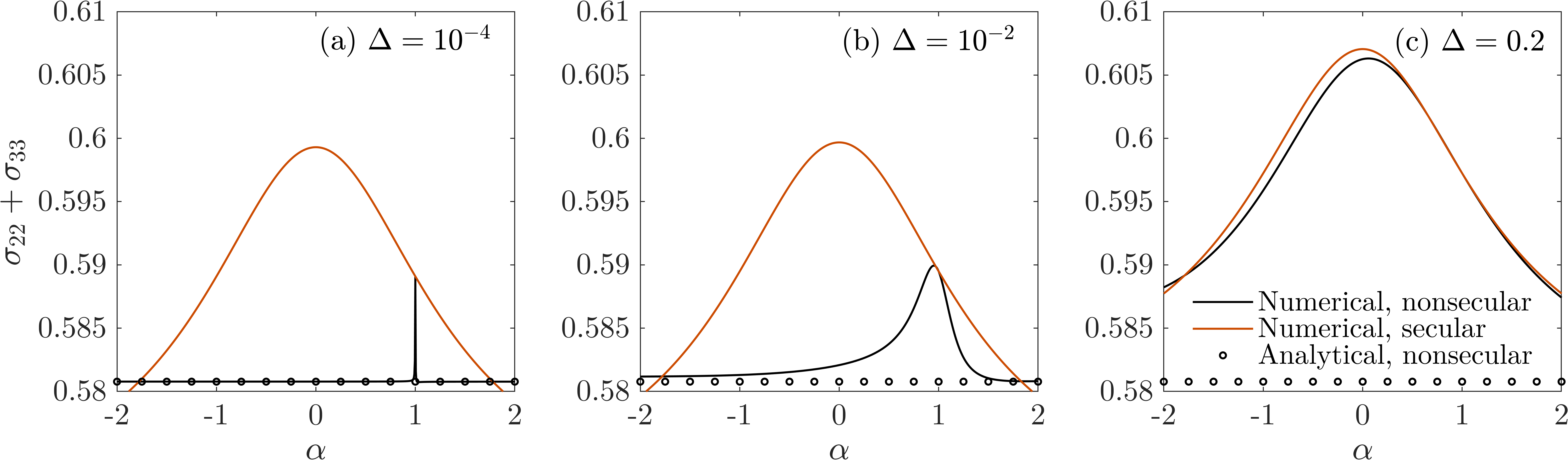
Figure 5: Steady state behavior of population. Plotted is the sum of excited state populations, $\sigma_{33}+\sigma_{22}$, as a function of $\alpha$ using the nonsecular Redfield analytically (dotted) and numerically (solid black) and secular Redfield numerically (solid grey). In panel (a) for $\Delta=10^{-4}$, numerical and analytical nonsecular Redfield gives the same constant $\sigma_{33}+\sigma_{22}$ as in Eq. (22) except at the anomalous point $\alpha=1$ where interestingly the nonsecular numerical Redfield result coincides with the secular. The numerical nonsecular results approaches the secular as $\Delta$ is increased, as shown in panel (b) where $\Delta=10^{-2}$ and (c) where $\Delta=0.2$. Other parameters are identical to Fig. 2.

V.2 Population

We now analyze excited state populations in steady state and demonstrate their dependence on the adjustable interference parameter, $\alpha$. Solving Eqs. (14) and (15) in steady state, together with Eq. (17), we obtain

$$\sigma_{22}=\frac{k_{c}(\alpha^{2}e^{-\beta_{h}\nu}+e^{-\beta_{c}\nu})+k_{h}(e^{-\beta_{c}\nu}+e^{-\beta_{h}\nu})}{\left[(\alpha^{2}+1)k_{c}+2k_{h})(e^{-\beta_{c}\nu}+e^{-\beta_{h}\nu}+1)\right]}+\mathcal{O}(\Delta^{2}),$$

(20)

and

$$\sigma_{33}=\frac{k_{c}(e^{-\beta_{h}\nu}+\alpha^{2}e^{-\beta_{c}\nu})+k_{h}(e^{-\beta_{c}\nu}+e^{-\beta_{h}\nu})}{\left[(\alpha^{2}+1)k_{c}+2k_{h})(e^{-\beta_{c}\nu}+e^{-\beta_{h}\nu}+1)\right]}+\mathcal{O}(\Delta^{2}).$$

(21)

The steady-state populations, $\sigma_{22}$, $\sigma_{33}$, and thus $\sigma_{11}$ are insensitive to the sign of $\alpha$. Furthermore, adding equations (20) and (21) reveals an analog to the so-called “population-locked-states” effect discussed e.g. in Ref. Kozlov, Rostovtsev, and Scully (2006),

$$P_{ex}\equiv\sigma_{22}+\sigma_{33}=\frac{e^{-\beta_{c}\nu}+e^{-\beta_{h}\nu}}{e^{-\beta_{c}\nu}+e^{-\beta_{h}\nu}+1}+\mathcal{O}(\Delta^{2}).$$ (22)

A fraction of the population, given by Eq. (22), is always shared between the two excited states, $|2\rangle$ and $|3\rangle$, independent of $\alpha$.

Complementing this analytical result, which is valid when $\Delta\to 0$, in Fig. 5 we present numerical simulations for $P_{ex}$ performed at finite $\Delta$. As $\Delta$ diminishes, we observe a sharp spike when approaching $\alpha=1$, at a point where strong interferences between two pathways takes place leading to zero coherences. Interestingly, at this point the total excited state population $P_{ex}$ coincides with the prediction of the secular equation. This anomaly is otherwise hidden in the $\mathcal{O}(\Delta^{2})$ term in Eq. (22) (the width of the spike depends on $\Delta$). As we increase $\Delta$, we find that the prediction of the secular method approaches the nonsecular result, while the analytic result Eq. (22), which relies on $\Delta\to 0$, naturally fails to capture the correct behavior of $P_{ex}$.

From Equations (20) and (21) we find that both excited states are equally populated when $\alpha=1$ or $\alpha=-1$, up to the first order in $\Delta$. . Therefore, we can write the state the of the nonequilibrium system as the algebraic average of the two thermal states,

$$\sigma(\alpha^{2}=1)=\frac{e^{-\hat{H}_{S}\beta_{h}}+e^{-\hat{H}_{S}\beta_{c}}}{\text{Tr}_{S}[e^{-\hat{H}_{S}\beta_{h}}+e^{-\hat{H}_{S}\beta_{c}}]}+\mathcal{C}+\mathcal{O}(\Delta^{2}).$$ (23)

Here $\hat{H}_{S}$ is the system Hamiltonian of the fully degenerate V model; $\mathcal{C}$ contains the off-diagonal terms of the RDM. Furthermore, when $T_{h}\neq T_{c}$, we conclude from Eqs. (20) and (21) that

$$\alpha^{2}<1\Leftrightarrow\sigma_{22}<\sigma_{33}.$$ (24)

Thus, $\alpha$ can be tuned to force the system to exhibit population inversion at steady state (although the effect is small with our parameters as shown in Fig. 3). This observation is another nontrivial result of this work. When prepared in the ground state, dynamical simulations in Fig. 3 also show that there exists a time interval $\tau$ where $\sigma_{22}(\tau)<\sigma_{33}(\tau)$ before reaching $\sigma_{22}>\sigma_{33}$, and vice-versa.

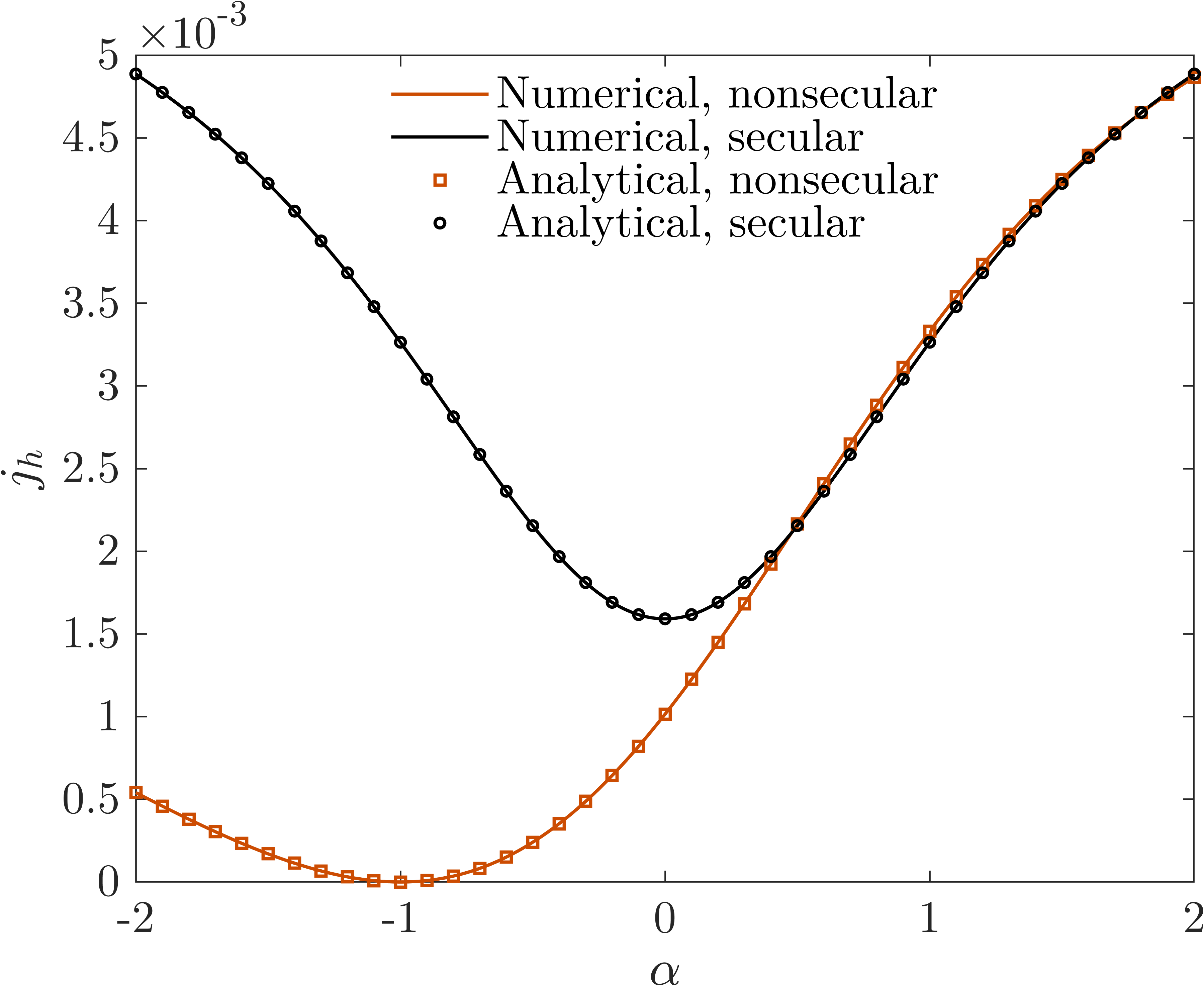
Figure 6: Steady-state heat current $j_{h}$ as a function of $\alpha$. We compare numerical simulations from the nonsecular secular (solid black) and Redfield equation (solid orange) to the analytical expressions (symbols), with Eqs. (V.3) and (27), respectively. Parameters are the same as in Fig. 2.

V.3 Heat current

The heat currents $j_{h,c}$ are evaluated at the hot and cold contacts, respectively, using the dissipators, see Eq. (11). Specifically at the hot contact,

$$j_{h}=\nu\mathcal{D}^{h}_{33}(\sigma)+(\nu-\Delta)\mathcal{D}^{h}_{22}(\sigma).$$ (25)

Inserting the solutions for the coherences, Eq. (18), and the populations, Eqs. (20) and (21) into the dissipator, we get

$$j_{h}=\nu\frac{(1+\alpha)^{2}(k_{h}k_{c})(e^{-\beta_{h}\nu}-e^{-\beta_{c}\nu})}{\left[(\alpha^{2}+1)k_{c}+2k_{h}\right](e^{-\beta_{c}\nu}+e^{-\beta_{h}\nu}+1)}+\mathcal{O}(\Delta).$$

By making the substitution Eq. (12) we highlight that the steady state current is non-vanishing when $T_{h}\neq T_{c}$ and $\alpha\neq-1$, and obtain Eq. (2). Note that the $\alpha$-dependence cancels out in Eq. (V.3) when $\alpha k_{c}=k_{h}$, a point at which one of the pathways becomes equilibrium-like.

Equation (V.3), or in its microscopic form, Eq. (2), complements our expressions for the coherences and populations, and it is another central result of this work. We expect that it will be used as the groundwork for more involved studies, e.g., when studying thermal energy transport at strong coupling. We plot the steady-state heat current in Fig. 6, showing that the above expression is accurate for quasi-degenerate excited states. Inspecting Eq. (V.3) and Fig. 6, we observe the following:

(i) The nonsecular heat current is not an even function of $\alpha$, a clear indication that quantum coherences are at play, with the sign of $\alpha$ playing a role in transport. In contrast, under the secular approximation, the current is symmetric in $\alpha$.

(ii) The $[e^{-\beta_{h}\nu}-e^{-\beta_{c}\nu}]$ factor in the numerator exposes the trivial dependence of the heat current on the temperature difference.

(iii) Given the structure of the denominator, it is clear that exchanging the temperatures of the two baths should lead to a thermal diode effect, since the current is not identical under the $k_{h}\leftrightarrow k_{c}$ operation (except for $|\alpha|=1$). We discuss this aspect in Sec. VI.

(iv) The steady state heat current is high when quantum coherences are low, and vice versa; compare Fig. 4 to Fig. 6.

(v) To the lowest order, the steady state heat current does not depend on the excited-state splitting $\Delta$. Similarly, the levels’ population and their coherences are independent of $\Delta$ to lowest order (assuming $\Delta\to 0$). Parameters that do dictate these functions are the spectral density function, temperature of the baths, and the overall splitting $\nu$. In stark contrast, the rise of coherences and the development of an extended transient region over which they survive is controlled by a timescale inversely proportional to $\Delta^{2}$, see Refs. Tscherbul and Brumer (2014, 2018); Dodin and Brumer (2021); Dodin et al. (2018); Dodin, Tscherbul, and Brumer (2016b); Koyu et al. (2021); com ; Dodin, Tscherbul, and Brumer (2016a). Thus, the lifetime of transient coherence, and their magnitude at steady state are dictated by a different set of parameters.

V.4 The secular approximation

The secular approximation decouples population dynamics and coherent dynamics, amounting to crossing out $\sigma_{32}(t)$ in Eqs. (14) and (15). It is justified when $\Delta$ is large such that the characteristic time of coherent oscillations is much shorter than the population decay time. The steady state solution thus involves a $2\times 2$ coefficient matrix for the population of the excited states. At steady state, the heat current is given by ($S$ stands for secular)

$$j_{h}^{S}=\frac{\nu k_{h}k_{c}(e^{-\beta_{h}\nu}-e^{-\beta_{c}\nu})\left[k_{h}(\alpha^{2}+1)+2\alpha^{2}k_{c}\right]}{(k_{h}+k_{c})(k_{h}+\alpha^{2}k_{c})+e^{-\beta_{h}\nu}(2k_{h}^{2}+k_{c}k_{h}+\alpha^{2}k_{c}k_{h})+e^{-\beta_{c}\nu}(2\alpha^{2}k_{c}^{2}+k_{c}k_{h}+\alpha^{2}k_{c}k_{h})}+\mathcal{O}(\Delta).$$ (27)

Most notably, this expression is even in $\alpha$, unlike the nonsecular result, Eq. (V.3), thus reflecting that only the magnitude of $\alpha$ controls the secular current, rather than its sign. This behavior is illustrated in Fig. 6. In the special cases $|\alpha|=1$, Eq. (27) reduces to

$$j_{h}^{S}(\alpha^{2}=1)=\frac{2\nu k_{h}k_{c}(e^{-\beta_{h}\nu}-e^{-\beta_{c}\nu})}{k_{h}(1+2e^{-\beta_{h}\nu})+k_{c}(1+2e^{-\beta_{c}\nu})}+\mathcal{O}(\Delta).$$

(28)

This expression recovers the result obtained in Ref Kilgour and Segal (2018) where $\alpha=-1$ was used throughout. Interestingly, Fig. 6 shows that the secular approximation works reasonably well when $\alpha\gtrsim 1$. Another nontrivial observation from Fig. 6 is that for a broad range of parameters, quantum coherences reduce the heat current in the V model, with the secular current exceeding the nonsecular one. Coherences are either noninfluential to the current, or they suppress it. This can be viewed as a coherent heat current flowing against the temperature difference Wang et al. (2018).

Figure 7: Schematic representation of the V model in the local site basis. In this picture, $\Delta/2$ is the tunneling energy between degenerate excited states. (left) The $\alpha=1$ case corresponds to a side-coupled model where only one transition, $|1\rangle\leftrightarrow|a\rangle$ is coupled to both heat baths, but the excited states are coherently coupled (dashed arrow). (right) The $\alpha=-1$ case corresponds to a serial model: Heat is absorbed in the $|1\rangle\leftrightarrow|a\rangle$ transition, it tunnels coherently to $|b\rangle$, and decays from there to the cold bath.

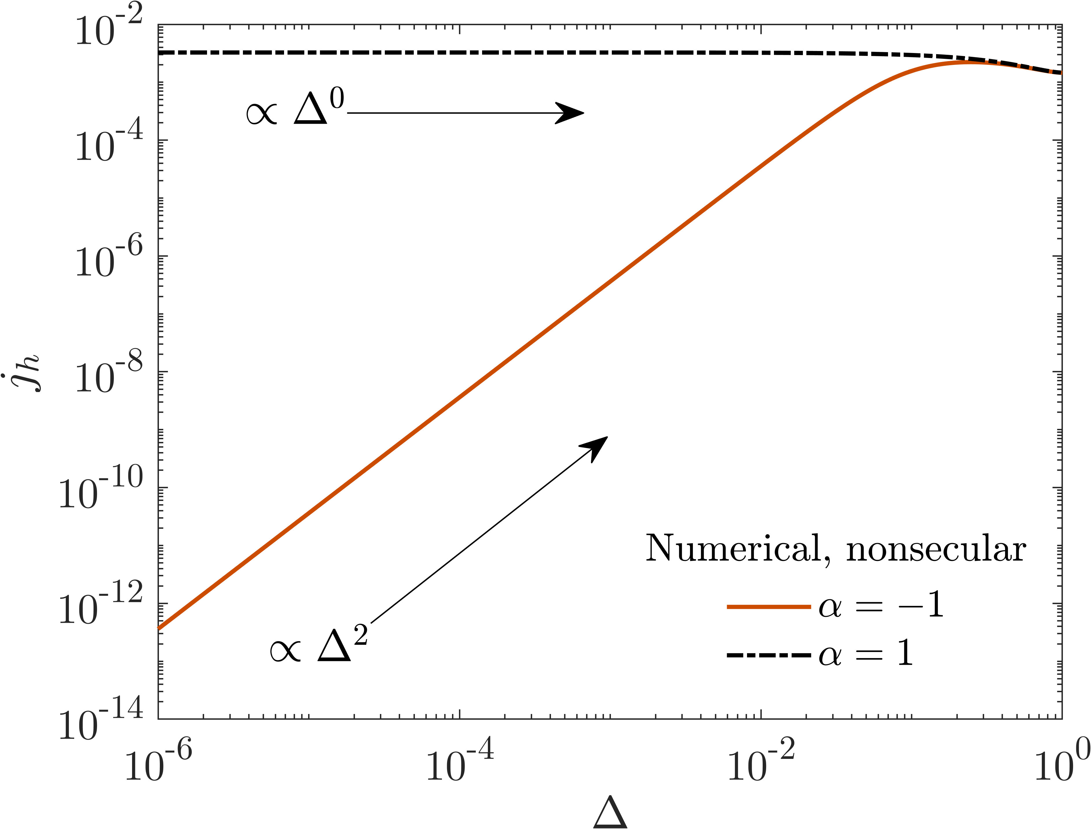
Figure 8: Steady-state heat current vs. excited state splitting $\Delta$ for $\alpha=-1$ (solid) and $\alpha=1$ (dashed-dotted). While in the former, $j_{h}\propto\Delta^{2}$ when $\Delta$ is small, in the latter case of $\alpha=1$ the current is nonzero (and independent of $\Delta$) even when $\Delta\to 0$. Other parameters are identical to Fig. 2.

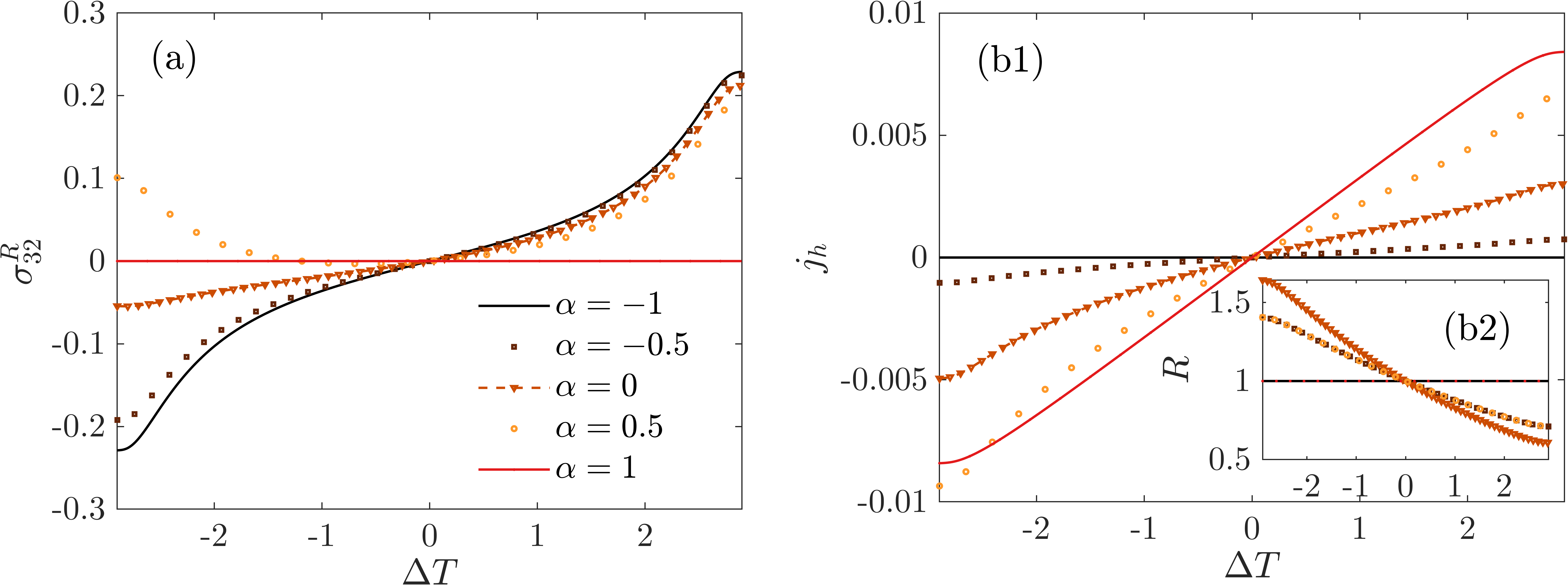
Figure 9: Control of thermal rectification by the coupling strength $\alpha$. (a) Coherences and (b1) heat current as a function of the temperature difference $\Delta T=T_{h}-T_{c}$. (b2) The rectification ratio $R=|j_{h}(\Delta T)/j_{h}(-\Delta T)|$ for different values of $\alpha$ ranging from $-1$ to $1$. Parameters are the same as in Fig. 2.

VI Discussion

VI.1 Quantum interferometers and local-basis mapping

The V model as depicted in Fig. 1 is analogous to a double quantum dot interferometer. However, instead of electron transport through two parallel dots, here thermal energy transfer takes place through quasi-degenerate excited states of frequencies $\nu-\Delta$ and $\nu$. In our work, the driving force for the transfer process are incoherent baths, rather than a coherent laser, but the mechanism is similar to Fano interferences Fano (1961), also considered in Refs. Scully et al. (2011); Dorfman et al. (2013); Svidzinsky, Dorfman, and Scully (2011); Tscherbul and Brumer (2018); Dodin and Brumer (2021); Dodin et al. (2018); Dodin, Tscherbul, and Brumer (2016b); Tscherbul and Brumer (2014); Dodin, Tscherbul, and Brumer (2016a); Koyu et al. (2021).

The effects observed in this work can be also rationalized without requiring interference arguments, by working in the local basis Kilgour and Segal (2018), referred to as the V-Energy Transfer System (VETS). The V model, Fig. 1, can be unitarily transformed into a local (L) picture,

$$\hat{H}_{S}^{L}=\left(\nu-\frac{\Delta}{2}\right)(|a\rangle\langle a|+|b\rangle\langle b|)+\frac{\Delta}{2}|a\rangle\langle b|+h.c.$$ (29)

The three levels in this system are the ground state $|1\rangle$ (same as in the energy basis) and the fully degenerate excited states $|a\rangle$ and $|b\rangle$ with the tunneling energy $\Delta/2$. This system couples to heat baths via

$$\hat{S}_{h}^{L} = |1\rangle\langle a|+h.c.$$

$$\hat{S}_{c}^{L} = \frac{1+\alpha}{2}|1\rangle\langle a|+\frac{\alpha-1}{2}|1\rangle\langle b|+h.c.,$$ (30)

see Appendix D for further details.

The two limiting configurations, $\alpha=1$ and $\alpha=-1$, are sketched in Fig. 7. The $\alpha=1$ case corresponds to a “side-coupled” model in the context of e.g. double quantum dots Barański et al. (2020). In this case, the transition $|1\rangle\leftrightarrow|a\rangle$ is driven by both heat baths, but level $|b\rangle$ is accessible only through a coherent coupling from level $|a\rangle$. In contrast, the $\alpha=-1$ case is reminiscent of a serial double dot model. Here, the ground state is coupled to level $|a\rangle$ through the hot heat bath. Since the two excited states are coherently coupled, energy transfers coherently from $|a\rangle$ to level $|b\rangle$, followed by a relaxation to the ground state and energy transfer to the cold bath using $\hat{S}_{c}^{L}$. In this picture, it is obvious that the heat current vanishes for $\alpha=-1$ once $\Delta=0$.

Consistent with this description, the steady-state heat currents in Fig. 8 demonstrate distinct scaling with $\Delta$ for $\alpha=-1$ and $\alpha=1$: In the former case, the current scales as $\Delta^{2}$. On the other hand, the $\alpha=1$ model only minimally depends on $\Delta$. Note that when $\Delta$ is very large (approaching the total gap $\nu$), deviations from these scaling are observed due to the large modification of energy levels, see Ref. Kilgour and Segal (2018).

Figure 10: Examination of thermodynamic consistencies in our work. (a) Energy conservation: The sum of heat currents $j_{h}(t)+j_{c}(t)$ approaches zero in the steady state limit. (b) Second law: The rate of entropy production $\dot{\Sigma}(t)=-j_{h}(t)/T_{h}-j_{c}(t)/T_{c}-\frac{d}{dt}\Tr{\sigma(t)\ln\sigma(t)}$ is always positive (note the log scale). (c1-3) Complete positivity: eigenvalues of the reduced density matrix $\sigma(t)$ demonstrate the preservation of trace and complete positivity for different values of $\alpha$ throughout the dynamical evolution. Parameters are the same as in Fig. 2.

VI.2 Thermal rectification

Thermal rectification is a transport phenomenon whereby the magnitude of the heat current is different upon exchanging the direction of the applied temperature bias. In the quantum domain, early proposals for a thermal diode (rectifier) were built on the nonequilibrium spin-boson model Segal and Nitzan (2005); Segal (2006). Recently, a quantum thermal diode was experimentally realized using superconducting quantum circuits Ronzani et al. (2018).

The diode effect is realized in systems that include (i) anharmonicity and (ii) asymmetry Ronzani et al. (2018); Wu and Segal (2009); Segal and Nitzan (2005); Segal (2006); Wu, Yu, and Segal (2009). Anharmonicity is captured in the V model due the three-level structure, distinct from the harmonic oscillator spectrum of the baths. Spatial asymmetry is introduced into the V model due to the imbalance between the arms, courtesy of the coherence parameter $\alpha$ Segal and Nitzan (2005). The figure of merit used to quantify the thermal diode effect is the rectification ratio, $R=\absolutevalue{\frac{j_{h}(\Delta T)}{j_{h}(-\Delta T)}}$, with rectification marked by $R\neq 1$.

For quasi-degenerate levels, $\Delta\to 0$, the nonequilibrium V system acts as a thermal diode once $\alpha\neq\pm 1$: For $\alpha=1$ (see Fig. 7), the model is spatially symmetric and thus trivially it cannot act as a diode. For $\alpha=-1$, the current itself vanishes when $\Delta\to 0$. The impact of interferences on thermal rectification and heat amplification was investigated in the fully degenerate nonequilibrium V model, by setting $\Delta$ to zero Wang et al. (2019). In contrast, in Fig 9 we study the diode effect in a nondegenerate system with tunable $\alpha$. We observe the following:

First, Fig 9(a) shows that steady-state coherences are asymmetric in $\alpha$, as was also observed in Fig. 4. Specifically, there are striking differences in the behavior of coherences with $\Delta T=T_{h}-T_{c}$ between $\alpha=-0.5$ and $\alpha=0.5$: While in the former, coherences increase monotonically with $\Delta T$, this is not the case for the latter. Second, a larger temperature bias produces greater coherences in absolute value. Third, there is an asymmetry in the magnitude of coherences with respect to temperature biases: a positive bias mostly produces larger coherences than a negative temperature bias.

Next, in Fig 9(b1)-(b2) we focus on the heat current and the rectification ratio. For $\alpha=\pm 1$, no rectification is observed. For intermediate values of $\alpha$, rectification behavior is observed, and is maximal when $\alpha=0$. Regardless, rectification ratios achieved in this model are rather modest, reaching at most $R\sim 1.7$. It remains a challenge to realize a significant nanoscale quantum thermal rectifier.

VI.3 Thermodynamic consistency of the Redfield equation for the V model

Quantum master equations in the Redfield form are known to exhibit pathologies Suárez, Silbey, and Oppenheim (1992); Kohen, Marston, and Tannor (1997); Cheng and Silbey (2005). Most notably, the Redfield equation is in principle not a completely-positive and trace preserving map Hartmann and Strunz (2020), allowing violations of thermodynamic laws as observed in the transient domain Argentieri et al. (2014, 2015). To support our analysis in this paper, in Fig. 10 we study properties of the Redfield quantum master equation for the V model, demonstrating numerically the thermodynamic consistency of our results.

First, in Fig. 10(a) we test the conservation of energy by studying the sum of the two heat currents, $j_{h}(t)+j_{c}(t)$ for different values of $\alpha$. Recall our sign convention: currents are positive when flowing towards the system. In the steady state limit, we find that this sum approaches zero, validating the first law of thermodynamics of energy conservation. Next, in Fig. 10(b) we test the second law by displaying the entropy production rate $\dot{\Sigma}(t)$ as a function of time, $\dot{\Sigma}(t)=-\frac{j_{h}(t)}{T_{h}}-\frac{j_{c}(t)}{T_{c}}-\frac{d}{dt}\Tr{\sigma(t)\ln\sigma(t)}$. Throughout the time evolution, the entropy production rate is positive, and thus the system obeys the second law. Finally, in Fig. 10 (c1)-(c3) we test whether for the V model the Redfield equation is a completely-positive trace-preserving map. We find that throughout the dynamical evolution, the eigenvalues of the reduced density matrix are strictly positive, ensuring complete positivity. The sum of the eigenvalues is unity, implying trace preservation. Pathologies associated with the Redfield equation therefore do not manifest in the V model for the studied parameters.

VII Summary

We studied a quantum thermal junction in which quantum coherences play a decisive role. While in the popular nonequilibrium spin-boson nanojunction coherences in the system do not alter transport (in the weak system-bath coupling limit), in the V model coherences are generated by the nonequilibrium heat baths, and their transient and steady state behavior go hand in hand with that of the heat current. Our main achievements are:

(i) In the limit of quasi-degenerate excited states we used the nonsecular Redfield equation and derived closed-form expressions in steady state identifying conditions for nonzero coherences and heat currents with a tunable interference parameter $\alpha$. We found that quantum coherences were non-vanishing in the steady-state limit due to a combination of coherent and incoherent factors: (a) the V model was in a nonequilibrium steady-state, (b) the parallel transport pathways did not destructively interfere, and (c) the parallel pathways did not cancel out due to an effective equilibrium condition on one of the arms. Quantum coherences were generated and sustained in our model due to the incoherent baths, and this method may find practical applications in emerging quantum information technologies.

(ii) The Redfield approach is more cumbersome to handle than the Lindblad equation, and in principle is not always granted the luxury of complete positivity. Here we numerically showed that for the V model and the examined parameters, the Redfield map was completely positive and trace preserving.

(iii) By studying the behavior of the heat current under the secular approximation we identified physics missed by making this common approximation.

(iv) While our focus has been on the steady-state limit, we had further performed numerical simulations in the transient domain. We found that the behavior of coherences in the transient regime was markedly different compared to the steady state limit, indicating that different physical factors were at play. Indeed, while the timescale of the transient dynamics is inversely related to $\Delta^{2}$, see Refs Tscherbul and Brumer (2014, 2018); Dodin and Brumer (2021); Dodin et al. (2018); Dodin, Tscherbul, and Brumer (2016b); Koyu et al. (2021); com ; Dodin, Tscherbul, and Brumer (2016a), steady state coherences, population and currents only secondarily-negligibly depended on $\Delta$ in the quasi-degenerate limit.

In sum, we derived a closed-form expression for the heat current, Eq. (V.3), which depended on the quantum interference control parameter ($\alpha$). We expect that this analytical result will serve as a starting point for additional investigations of quantum coherence effects in thermal transport. Open experimental challenges include the construction of phase-controlled quantum thermal devices realizing this system with generalized complex couplings Fornieri and Giazotto (2017). From the theory side, open questions concern the interplay of quantum coherences and non-Markovianity, understanding the impact of strong system-bath coupling on quantum coherences, and uncovering the relationship between quantum coherences and fluctuations.

Appendix A: Redfield equation for the V model

The general form of the Redfield quantum master equation is given in Eq. (8). For the V model as presented in Eqs. (3)-(7), the surviving terms are

$$\dot{\sigma}_{32}(t) = -i\Delta\sigma_{32}(t)+\sum_{m}\Big{[}[R^{m}_{12,31}(\omega_{13})+R^{*,m}_{13,21}(\omega_{12})]\sigma_{11}(t)$$ (A1)

$$-[R^{m}_{31,13}(\omega_{31})+R^{*,m}_{21,12}(\omega_{21})]\sigma_{32}(t)-R^{m}_{31,12}(\omega_{21})\sigma_{22}(t)-R^{*,m}_{21,13}(\omega_{31})\sigma_{33}(t)\Big{]},$$

$$\dot{\sigma}_{22}(t) = \sum_{m}\Big{[}[R^{m}_{12,21}(\omega_{12})+R^{*,m}_{12,21}(\omega_{12})]\sigma_{11}(t)$$ (A2)

$$- [R^{m}_{21,12}(\omega_{21})+R^{*,m}_{21,12}(\omega_{21})]\sigma_{22}(t)-R^{m}_{21,13}(\omega_{31})\sigma_{32}(t)-R^{*,m}_{21,13}(\omega_{31})\sigma_{23}(t)\Big{]},$$

and

$$\dot{\sigma}_{33}(t) = \sum_{m}\Big{[}[R^{m}_{13,31}(\omega_{13})+R^{*,m}_{13,31}(\omega_{13})]\sigma_{11}(t)$$ (A3)

$$- [R^{m}_{31,13}(\omega_{31})+R^{*,m}_{31,13}(\omega_{31})]\sigma_{33}(t)-R^{m}_{31,12}(\omega_{21})\sigma_{23}(t)-R^{*,m}_{31,12}(\omega_{21})\sigma_{32}(t)\Big{]},$$

where $m=h,c$ is the index for the heat bath and the frequencies are calculated from the eigenenergies of the system, $\omega_{ij}=E_{i}-E_{j}$. Note that by construction, there are no coherence terms between the ground state and the excited states. To calculate the dissipator, we use Eq. (9) ignoring the so-called Lamb shifts, an approximation that should be valid when $T>\Delta$. We further make use of the detailed-balance relation and write all rates in terms of bath-induced decay rates, $k(\omega)$ with $\omega>0$ [see Eq. (10)]. The coherences satisfy

$$\dot{\sigma}_{32}(t)= - i\Delta\sigma_{32}(t)-\frac{1}{2}\left[k_{h}(\omega_{31})+k_{h}(\omega_{21})+\alpha^{2}k_{c}(\omega_{31})+k_{c}(\omega_{21})\right]\sigma_{32}(t)$$ (A4)

$$- \frac{1}{2}\left[k_{h}(\omega_{21})+\alpha k_{c}(\omega_{21})\right]\sigma_{22}(t)-\frac{1}{2}\left[k_{h}(\omega_{31})+\alpha k_{c}(\omega_{31})\right]\sigma_{33}(t)$$

$$+ \frac{1}{2}\left[k_{h}(\omega_{31})e^{-\beta_{h}\omega_{31}}+k_{h}(\omega_{21})e^{-\beta_{h}\omega_{21}}+\alpha k_{c}(\omega_{31})e^{-\beta_{c}\omega_{31}}+\alpha k_{c}(\omega_{21})e^{-\beta_{c}\omega_{21}}\right]\sigma_{11}(t).$$

The excited state population dynamics includes gain-loss terms from-to the ground state, as well as the coupling to coherences,

$$\dot{\sigma}_{22}(t) = -\left[k_{h}(\omega_{21})+k_{c}(\omega_{21})\right]\sigma_{22}(t)+\left[k_{h}(\omega_{21})e^{-\beta_{h}\omega_{21}}+k_{c}(\omega_{21})e^{-\beta_{c}\omega_{21}}\right]\sigma_{11}(t)$$ (A5)

$$-\left[k_{h}(\omega_{31})+\alpha k_{c}(\omega_{31})\right]\sigma_{32}^{R}(t).$$

A similar equation of motion holds for the other excited state,

$$\dot{\sigma}_{33}(t) = -\left[k_{h}(\omega_{31})+\alpha^{2}k_{c}(\omega_{31})\right]\sigma_{33}(t)+\left[k_{h}(\omega_{31})e^{-\beta_{h}\omega_{31}}+\alpha^{2}k_{c}(\omega_{31})e^{-\beta_{c}\omega_{31}}\right]\sigma_{11}(t)$$ (A6)

$$-\left[k_{h}(\omega_{21})+\alpha k_{c}(\omega_{21})\right]\sigma_{32}^{R}(t).$$

We recall that these equations rely on (i) the Born-Markov approximation and (ii) the omission of the imaginary part of the rates (“Lamb shifts”). However, unlike the Lindblad form, the equations arise from microscopic principles and they are nonsecular. Simulations presented in the main text are based on solving numerically equations (A4)-(A6).

To solve these equations analytically, further simplifications are necessary. Working in the limit of nearly-degenerate excited levels, $\Delta\to 0$, we make an additional approximation for the thermally-induced decay rates, $k_{h}(\omega_{31})\approx k_{h}(\omega_{21})$, denoted in short by $k_{h}$. A similar approximation is made for $k_{c}$. All rates are now evaluated at the transition energy $\nu$, see Fig. 1. However, the unitary term $i\Delta\sigma_{32}(t)$ in Eq. (A4) is kept intact. The resulting simplified equations are presented in Eqs. (13)-(15). In steady state, after using the population normalization condition, we recast the system in an algebraic form as

$$0=\mathcal{M}\vec{v}+\vec{d},$$ (A7)

with the steady state solution $\vec{v}\equiv[\sigma_{22}\ \sigma_{33}\ \sigma_{32}^{R}]^{T}$. The matrix is

$$\mathcal{M}=-\begin{bmatrix}(e^{-\beta_{h}\nu}+1)k_{h}+(e^{-\beta_{c}\nu}+1)k_{c}&e^{-\beta_{h}\nu}k_{h}+e^{-\beta_{c}\nu}k_{c}&k_{h}+\alpha k_{c}\\ e^{-\beta_{h}\nu}k_{h}+\alpha^{2}e^{-\beta_{c}\nu}k_{c}&(e^{-\beta_{h}\nu}+1)k_{h}+\alpha^{2}(e^{-\beta_{c}\nu}+1)k_{c}&k_{h}+\alpha k_{c}\\ \alpha\frac{k_{c}(1+2e^{-\beta_{c}\nu})}{2}+\frac{k_{h}(1+2e^{-\beta_{c}\nu})}{2}&\alpha\frac{k_{c}(1+2e^{-\beta_{c}\nu})}{2}+\frac{k_{h}(1+2e^{-\beta_{c}\nu})}{2}&\xi+\Delta^{2}/\xi\end{bmatrix},$$ (A8)

and the constant terms are

$$\vec{d}=\begin{bmatrix}e^{-\beta_{h}\nu}k_{h}+e^{-\beta_{c}\nu}k_{c}\,\,\,\,\,\,&e^{-\beta_{h}\nu}k_{h}+\alpha^{2}e^{-\beta_{c}\nu}k_{c}\,\,\,\,\,\,&e^{-\beta_{h}\nu}k_{h}+\alpha e^{-\beta_{c}\nu}k_{c}\end{bmatrix}^{T}$$ (A9)

The steady state solution is obtained by inverting the coefficient matrix $\mathcal{M}$.

To obtain the analogous set of secular equations, coherent terms are set to vanish in Eqs. (A5) and (A6) then we proceed as with the nonsecular analog to obtain Eq. (27). For completeness, we provide here expressions for population,

$$\sigma_{22}^{S}=\frac{(k_{c}\alpha^{2}+k_{h})(e^{-\beta_{c}\nu}k_{c}+e^{-\beta_{h}\nu}k_{h})}{\text{Det[}\mathcal{M}^{S}]}$$ (A10)

and

$$\sigma_{33}^{S}=\frac{(k_{c}+k_{h})(e^{-\beta_{c}\nu}k_{c}\alpha^{2}+e^{-\beta_{h}\nu}k_{h})}{\text{Det[}\mathcal{M}^{S}]}$$ (A11)

with

$$\text{Det[}\mathcal{M}^{S}] = \Big{[}k_{h}(1+e^{-\beta_{h}\nu})+k_{c}(1+e^{-\beta_{c}\nu})\Big{]}\Big{[}k_{h}(1+e^{-\beta_{h}\nu})+\alpha^{2}k_{c}(1+e^{-\beta_{c}\nu})\Big{]}$$ (A12)

$$- \Big{(}k_{h}e^{-\beta_{h}\nu}+k_{c}e^{-\beta_{c}\nu}\Big{)}\Big{(}k_{h}e^{-\beta_{h}\nu}+\alpha^{2}k_{c}e^{-\beta_{c}\nu}\Big{)},$$

where recall that the $S$ superscript denotes the secular limit.

Appendix B: Equilibrium single-bath V model

Here, we investigate the V model when coupled to a single bath. In this case, the system is expected to equilibrate to a Gibbs state in the long time limit. Explicitly, we set $k_{c}=0$ in Eqs. (13)-(15) and $k_{h}=k$ as the decay rate,

$$\dot{\sigma}_{32}(t) = -i\Delta\sigma_{32}(t)-k\sigma_{32}(t)-\frac{1}{2}k\left[\sigma_{22}(t)+\sigma_{33}(t)\right]+ke^{-\beta\nu}\sigma_{11}(t),$$ (B1)

$$\dot{\sigma}_{22}(t) = -k\sigma_{22}(t)+ke^{-\beta\nu}\sigma_{11}(t)-k\sigma_{32}^{R}(t),$$ (B2)

$$\dot{\sigma}_{33}(t) = -k\sigma_{33}(t)+ke^{-\beta\nu}\sigma_{11}(t)-k\sigma_{32}^{R}(t).$$ (B3)

These equations of motion map to a limiting configuration of Eqs. (1a) and (1b) of Ref. Dodin, Tscherbul, and Brumer (2016a) as follows. First, in their notation, $r=r_{1}=r_{2}$ is the pumping rate while $\gamma=\gamma_{1}=\gamma_{2}$ is the spontaneous decay rate.

To match the equations (note that their physical scenario is distinct), we identify our decay rate by $k=r+\gamma$ with $r=2J(\nu)n(\nu)$ and $\gamma=2J(\nu)$. Since $k=2J(\nu)[n(\nu)+1]$, we conclude that $r=ke^{-\beta\nu}$. Recall that $J(\nu)$ is the spectral density of the bath and $n(\nu)$ is the Bose-Einstein function. Further setting $p=1$ we get

$$\dot{\sigma}_{22}(t) = -(r+\gamma)\sigma_{22}(t)+r\sigma_{11}(t)-(r+\gamma)\sigma_{32}^{R}(t)$$

$$\dot{\sigma}_{33}(t) = -(r+\gamma)\sigma_{33}(t)+r\sigma_{11}(t)-(r+\gamma)\sigma_{32}^{R}(t)$$

$$\dot{\sigma}_{32}(t) = -(r+\gamma+i\Delta)\sigma_{32}^{R}(t)+r\sigma_{11}(t)-\frac{r+\gamma}{2}(\sigma_{22}(t)+\sigma_{33}(t)).$$ (B4)

These equations are indeed identical to those presented in Ref. Dodin, Tscherbul, and Brumer (2016a).

We now recast equation (B4) in a matrix form (after applying the normalization condition $1=\sigma_{11}(t)+\sigma_{22}(t)+\sigma_{33}(t)$), $\dot{{\vec{v}}}(t)=\mathcal{M}\vec{v}(t)+\vec{d}$ with $\vec{v}(t)\equiv[\sigma_{22}(t)\ \sigma_{33}(t)\ \sigma_{32}^{R}(t)\ \sigma_{32}^{I}(t)]^{T}$, $\vec{d}\equiv r[1\ 1\ 1\ 0]^{T}$ and the matrix

$$\mathcal{M}=\begin{bmatrix}-(2r+\gamma)&-r&-(r+\gamma)&0\\ -r&-(2r+\gamma)&-(r+\gamma)&0\\ -\frac{1}{2}(3r+\gamma)&-\frac{1}{2}(3r+\gamma)&-(r+\gamma)&\Delta\\ 0&0&-\Delta&-(r+\gamma)\\ \end{bmatrix}.$$ (B5)

This equation is distinct from Eq. (2b) of Ref. Dodin, Tscherbul, and Brumer (2016a), apparently due to a typo there.

We make use of existing symmetry in the system by defining $P(t)\equiv\frac{1}{2}(\sigma_{22}(t)+\sigma_{33}(t))$ such that

$$\dot{P}(t)=-k\sigma_{32}^{R}(t)-\phi P(t)+(\phi-k)/2$$ (B6)

$$\dot{\sigma}_{32}^{R}(t)=-k\sigma_{32}^{R}(t)-\phi P(t)+\Delta\sigma_{32}^{I}(t)+(\phi-k)/2$$ (B7)

$$\dot{\sigma}_{32}^{I}(t)=-k\sigma_{32}^{I}(t)-\Delta\sigma_{32}^{R}(t),$$ (B8)

where $\phi\equiv(1+2e^{-\beta\nu})k$. Note that no further approximations were made to obtain Eqs. (B6)-(B8) from Eqs. (B1)-(B3). The unique set of steady-state solutions $\sigma_{32}^{R}=\sigma_{32}^{I}=0$ and $P=\frac{\phi-k}{2\phi}$ clearly satisfies Eq. (B6)-(B8) in the steady-state limit. This solution for the steady-state populations is exactly the Gibbs state with the bath’s temperature.

Appendix C: The nonequilibrium V model at $\alpha=1$

As we show in Fig. 4 and Eq. (18), out of equilibrium baths generate and sustain coherences in the excited states in the steady state limit, but this coherence nullifies when $\alpha=1$. We now show that the equations of motion at $\alpha=1$ map to the single-bath case.

We simplify Eqs. (13)-(15) by setting $\alpha=1$,

$$\dot{\sigma}_{32}(t) = -i\Delta\sigma_{32}(t)-\left(k_{h}+k_{c}\right)\sigma_{32}(t)-\frac{1}{2}\left(k_{h}+k_{c}\right)\left[\sigma_{22}(t)+\sigma_{33}(t)\right]+\left(k_{h}e^{-\beta_{h}\nu}+k_{c}e^{-\beta_{c}\nu}\right)\sigma_{11}(t)$$ (C1)

$$\dot{\sigma}_{22}(t) = -\left(k_{h}+k_{c}\right)\sigma_{22}(t)+\left(k_{h}e^{-\beta_{h}\nu}+k_{c}e^{-\beta_{c}\nu}\right)\sigma_{11}(t)-\left(k_{h}+k_{c}\right)\sigma_{32}^{R}(t)$$ (C2)

$$\dot{\sigma}_{33}(t) = -\left(k_{h}+k_{c}\right)\sigma_{33}(t)+\left(k_{h}e^{-\beta_{h}\nu}+k_{c}e^{-\beta_{c}\nu}\right)\sigma_{11}(t)-\left(k_{h}+k_{c}\right)\sigma_{32}^{R}(t).$$ (C3)

We now define $P(t)=(\sigma_{22}(t)+\sigma_{33}(t))/2$ and retrieve, remarkably, Eq. (B6)-(B8) with analogous analytical solutions yet identifying $k\equiv k_{h}+k_{c}$ and $\phi\equiv(1+2e^{-\beta_{h}\nu})k_{h}+(1+2e^{-\beta_{c}\nu})k_{c}$. We thus showed that the dynamics of the $\alpha=1$ case, with nonequilibrium baths, can be mapped to a single bath scenario (though the current in the former is non-vanishing at $\alpha=1$).

Appendix D: Local picture for the V model

In this Appendix we provide more details on the transformation between the V model in the energy basis and a particular local basis picture as discussed in Ref. Kilgour and Segal (2018).

In the local basis, $|1\rangle$ denotes the ground state and $|a\rangle$ and $|b\rangle$ are exactly-degenerate upper states, which are coherently coupled with the tunneling energy $\Delta/2$. It can be shown that the local Hamiltonian

$$\hat{H}_{S}^{L}=\begin{bmatrix}0&0&0\\ 0&\nu-\Delta/2&\Delta/2\\ 0&\Delta/2&\nu-\Delta/2\\ \end{bmatrix}$$ (D1)

is diagonalized via the transformation $\hat{H}_{S}^{L}=\hat{U}\hat{H}_{S}\hat{U}^{\dagger}$ with the unitary matrix

$$\hat{U}=\sqrt{\frac{1}{2}}\begin{bmatrix}1&0&0\\ 0&-1&1\\ 0&1&1\\ \end{bmatrix}$$ (D2)

The eigenvalue matrix corresponds to the V model (“global”) Hamiltonian Eq. (3). The system operators that couple to the baths go through the same transformation yielding the system-bath coupling operators in the local basis,

$$\hat{S}_{h}^{L}=\hat{U}\hat{S}_{h}\hat{U}^{\dagger} = |1\rangle\langle a|+|a\rangle\langle 1|,$$

$$\hat{S}_{c}^{L}=\hat{U}\hat{S}_{c}\hat{U}^{\dagger} = \frac{1+\alpha}{2}|1\rangle\langle a|+\frac{\alpha-1}{2}|1\rangle\langle b|+h.c.,$$ (D3)

While the hot bath allows only the transition from the ground state to $|a\rangle$, depending on $\alpha$, the cold bath may allow transitions to both excited states.

The limit $\alpha=1$ corresponds to the “side-coupled model” as level $|b\rangle$ does not couple to the ground state. In contrast when $\alpha=-1$ we reach the scenario of Ref. Kilgour and Segal (2018) where each excited state couples to the ground state through a different bath. In the latter case the tunneling energy $\Delta$ is essential for allowing energy transfer thus the current vanishes when $\Delta\to 0$ Kilgour and Segal (2018).

References

- Nielsen and Chuang (2010) M. A. Nielsen and I. L. Chuang, Quantum Computation and Quantum Information: 10th Anniversary Edition (Cambridge University Press, 2010).
- Engel et al. (2007) G. S. Engel, T. R. Calhoun, E. L. Read, T.-K. Ahn, T. Mančal, Y.-C. Cheng, R. E. Blankenship, and G. R. Fleming, “Evidence for wavelike energy transfer through quantum coherence in photosynthetic systems,” Nature 446, 782–786 (2007).
- Vaziri and Plenio (2010) A. Vaziri and M. B. Plenio, “Quantum coherence in ion channels: resonances, transport and verification,” New Journal of Physics 12, 085001 (2010).
- Engel (2011) G. S. Engel, “Quantum coherence in photosynthesis,” Procedia Chemistry 3, 222–231 (2011), 22nd Solvay Conference on Chemistry.
- Chin, Huelga, and Plenio (2012) A. W. Chin, S. F. Huelga, and M. B. Plenio, “Coherence and decoherence in biological systems: principles of noise-assisted transport and the origin of long-lived coherences,” Philosophical Transactions of the Royal Society A: Mathematical, Physical and Engineering Sciences 370, 3638–3657 (2012).
- Kassal, Yuen-Zhou, and Rahimi-Keshari (2013) I. Kassal, J. Yuen-Zhou, and S. Rahimi-Keshari, “Does coherence enhance transport in photosynthesis?” The Journal of Physical Chemistry Letters 4, 362–367 (2013).
- QB (2014) Quantum Effects in Biology (Cambridge University Press, 2014).
- Duan et al. (2017) H.-G. Duan, V. I. Prokhorenko, R. J. Cogdell, K. Ashraf, A. L. Stevens, M. Thorwart, and R. J. D. Miller, “Nature does not rely on long-lived electronic quantum coherence for photosynthetic energy transfer,” Proceedings of the National Academy of Sciences 114, 8493–8498 (2017).
- Gauger et al. (2011) E. M. Gauger, E. Rieper, J. J. L. Morton, S. C. Benjamin, and V. Vedral, “Sustained quantum coherence and entanglement in the avian compass,” Phys. Rev. Lett. 106, 040503 (2011).
- Pauls et al. (2013) J. A. Pauls, Y. Zhang, G. P. Berman, and S. Kais, “Quantum coherence and entanglement in the avian compass,” Phys. Rev. E 87, 062704 (2013).
- Smith, Deviers, and Kattnig (2022) L. D. Smith, J. Deviers, and D. R. Kattnig, “Observations about utilitarian coherence in the avian compass,” Scientific Reports 12, 6011 (2022).
- Prokhorenko et al. (2006) V. I. Prokhorenko, A. M. Nagy, S. A. Waschuk, L. S. Brown, R. R. Birge, and R. J. D. Miller, “Coherent control of retinal isomerization in bacteriorhodopsin,” Science 313, 1257–1261 (2006).
- Tscherbul and Brumer (2015) T. V. Tscherbul and P. Brumer, “Quantum coherence effects in natural light-induced processes: cis–trans photoisomerization of model retinal under incoherent excitation,” Phys. Chem. Chem. Phys. 17, 30904–30913 (2015).
- Dodin and Brumer (2019) A. Dodin and P. Brumer, “Light-induced processes in nature: Coherences in the establishment of the nonequilibrium steady state in model retinal isomerization,” The Journal of Chemical Physics 150, 184304 (2019).
- Latune, Sinayskiy, and Petruccione (2020) C. L. Latune, I. Sinayskiy, and F. Petruccione, “Negative contributions to entropy production induced by quantum coherences,” Phys. Rev. A 102, 042220 (2020).
- Scully et al. (2011) M. O. Scully, K. R. Chapin, K. E. Dorfman, M. B. Kim, and A. Svidzinsky, “Quantum heat engine power can be increased by noise-induced coherence,” Proceedings of the National Academy of Sciences 108, 15097–15100 (2011).
- Dorfman et al. (2013) K. E. Dorfman, D. V. Voronine, S. Mukamel, and M. O. Scully, “Photosynthetic reaction center as a quantum heat engine,” Proceedings of the National Academy of Sciences 110, 2746–2751 (2013).
- Scully et al. (2003) M. O. Scully, M. S. Zubairy, G. S. Agarwal, and H. Walther, “Extracting work from a single heat bath via vanishing quantum coherence,” Science 299, 862–864 (2003).
- Quan, Zhang, and Sun (2006) H. T. Quan, P. Zhang, and C. P. Sun, “Quantum-classical transition of photon-carnot engine induced by quantum decoherence,” Phys. Rev. E 73, 036122 (2006).
- De Liberato and Ueda (2011) S. De Liberato and M. Ueda, “Carnot’s theorem for nonthermal stationary reservoirs,” Phys. Rev. E 84, 051122 (2011).
- Liu and Segal (2021) J. Liu and D. Segal, “Coherences and the thermodynamic uncertainty relation: Insights from quantum absorption refrigerators,” Phys. Rev. E 103, 032138 (2021).
- Svidzinsky, Dorfman, and Scully (2011) A. A. Svidzinsky, K. E. Dorfman, and M. O. Scully, “Enhancing photovoltaic power by Fano-induced coherence,” Phys. Rev. A 84, 053818 (2011).
- Uzdin, Levy, and Kosloff (2015) R. Uzdin, A. Levy, and R. Kosloff, “Equivalence of quantum heat machines, and quantum-thermodynamic signatures,” Phys. Rev. X 5, 031044 (2015).
- Chen, Gao, and Galperin (2017) F. Chen, Y. Gao, and M. Galperin, “Molecular heat engines: Quantum coherence effects,” Entropy 19 (2017), 10.3390/e19090472.
- Dorfman, Xu, and Cao (2018) K. E. Dorfman, D. Xu, and J. Cao, “Efficiency at maximum power of a laser quantum heat engine enhanced by noise-induced coherence,” Phys. Rev. E 97, 042120 (2018).
- Holubec and Novotný (2018) V. Holubec and T. Novotný, “Effects of noise-induced coherence on the performance of quantum absorption refrigerators,” Journal of Low Temperature Physics 192, 147–168 (2018).
- Holubec and Novotný (2019) V. Holubec and T. Novotný, “Effects of noise-induced coherence on the fluctuations of current in quantum absorption refrigerators,” The Journal of Chemical Physics 151, 044108 (2019).
- Klatzow et al. (2019) J. Klatzow, J. N. Becker, P. M. Ledingham, C. Weinzetl, K. T. Kaczmarek, D. J. Saunders, J. Nunn, I. A. Walmsley, R. Uzdin, and E. Poem, “Experimental demonstration of quantum effects in the operation of microscopic heat engines,” Phys. Rev. Lett. 122, 110601 (2019).
- Tajima and Funo (2021) H. Tajima and K. Funo, “Superconducting-like heat current: Effective cancellation of current-dissipation trade-off by quantum coherence,” Phys. Rev. Lett. 127, 190604 (2021).
- Dag̃ et al. (2016) C. B. Dag̃, W. Niedenzu, O. E. Müstecaplıog̃lu, and G. Kurizki, “Multiatom quantum coherences in micromasers as fuel for thermal and nonthermal machines,” Entropy 18 (2016).
- Boller, Imamoğlu, and Harris (1991) K.-J. Boller, A. Imamoğlu, and S. E. Harris, “Observation of electromagnetically induced transparency,” Phys. Rev. Lett. 66, 2593–2596 (1991).
- Liu et al. (2001) C. Liu, Z. Dutton, C. Behroozi, and L. V. Hau, “Observation of coherent optical information storage in an atomic medium using halted light pulses,” Science 409, 490–493 (2001).
- Kang and Noh (2017) H.-J. Kang and H.-R. Noh, “Coherence effects in electromagnetically induced transparency in V-type systems of 87Rb,” Opt. Express 25, 21762–21774 (2017).
- Gray, Whitley, and Stroud (1978) H. R. Gray, R. M. Whitley, and C. R. Stroud, “Coherent trapping of atomic populations,” Opt. Lett. 3, 218–220 (1978).
- Kozlov, Rostovtsev, and Scully (2006) V. V. Kozlov, Y. Rostovtsev, and M. O. Scully, “Inducing quantum coherence via decays and incoherent pumping with application to population trapping, lasing without inversion, and quenching of spontaneous emission,” Phys. Rev. A 74, 063829 (2006).
- Xu et al. (2008) X. Xu, B. Sun, P. R. Berman, D. G. Steel, A. S. Bracker, D. Gammon, and L. J. Sham, “Coherent population trapping of an electron spin in a single negatively charged quantum dot,” Nature Physics 4, 692–695 (2008).
- Harris (1989) S. E. Harris, “Lasers without inversion: Interference of lifetime-broadened resonances,” Phys. Rev. Lett. 62, 1033–1036 (1989).
- Luo and Xu (1992) Z.-F. Luo and Z.-Z. Xu, “Lasing without inversion and coherence in dressed states,” Phys. Rev. A 45, 8292–8294 (1992).
- Scully and Fleischhauer (1994) M. O. Scully and M. Fleischhauer, “Lasers without inversion,” Science 263, 337–338 (1994).
- Scully and Zubairy (1997) M. O. Scully and M. S. Zubairy, Quantum Optics (Cambridge University Press, 1997).
- Braunstein and Shuker (2001) D. Braunstein and R. Shuker, “Absorption with inversion and amplification without inversion in a coherently prepared V system: A dressed-state approach,” Phys. Rev. A 64, 053812 (2001).
- Scully (2010) M. O. Scully, “Quantum photocell: Using quantum coherence to reduce radiative recombination and increase efficiency,” Phys. Rev. Lett. 104, 207701 (2010).
- Degen, Reinhard, and Cappellaro (2017) C. L. Degen, F. Reinhard, and P. Cappellaro, “Quantum sensing,” Rev. Mod. Phys. 89, 035002 (2017).
- Castellini et al. (2019) A. Castellini, R. Lo Franco, L. Lami, A. Winter, G. Adesso, and G. Compagno, “Indistinguishability-enabled coherence for quantum metrology,” Phys. Rev. A 100, 012308 (2019).
- Hegerfeldt and Plenio (1992) G. C. Hegerfeldt and M. B. Plenio, “Macroscopic dark periods without a metastable state,” Phys. Rev. A 46, 373–379 (1992).
- Hegerfeldt and Plenio (1993) G. C. Hegerfeldt and M. B. Plenio, “Coherence with incoherent light: A new type of quantum beat for a single atom,” Phys. Rev. A 47, 2186–2190 (1993).
- Menon and Agarwal (1999) S. Menon and G. S. Agarwal, “Probing the vacuum induced coherence in a -system,” (1999).
- Li, Peng, and Huang (2000) G. Li, J. Peng, and G. Huang, “Population inversion and absorption spectrum of a V-type three-level atom driven by coherent and stochastic fields,” Journal of Physics B: Atomic, Molecular and Optical Physics 33, 3743–3760 (2000).
- Ou, Liang, and Li (2008) B.-Q. Ou, L.-M. Liang, and C.-Z. Li, “Coherence induced by incoherent pumping field and decay process in three-level type atomic system,” Optics Communications 281, 4940–4945 (2008).
- Kiffner et al. (2010) M. Kiffner, M. Macovei, J. Evers, and C. Keitel, “Chapter 3 - vacuum-induced processes in multilevel atoms,” (Elsevier, 2010) pp. 85–197.
- Gelbwaser-Klimovsky et al. (2015) D. Gelbwaser-Klimovsky, W. Niedenzu, P. Brumer, and G. Kurizki, “Power enhancement of heat engines via correlated thermalization in a three-level “working fluid”,” Scientific Reports 5, 14413 (2015).
- Olšina et al. (2014) J. Olšina, A. G. Dijkstra, C. Wang, and J. Cao, “Can natural sunlight induce coherent exciton dynamics?” (2014).
- Tscherbul and Brumer (2014) T. V. Tscherbul and P. Brumer, “Long-lived quasistationary coherences in a -type system driven by incoherent light,” Phys. Rev. Lett. 113, 113601 (2014).
- Dodin, Tscherbul, and Brumer (2016a) A. Dodin, T. V. Tscherbul, and P. Brumer, “Quantum dynamics of incoherently driven V-type systems: Analytic solutions beyond the secular approximation,” The Journal of Chemical Physics 144, 244108 (2016a).
- Dodin, Tscherbul, and Brumer (2016b) A. Dodin, T. V. Tscherbul, and P. Brumer, “Coherent dynamics of V-type systems driven by time-dependent incoherent radiation,” The Journal of Chemical Physics 145, 244313 (2016b).
- Dodin et al. (2018) A. Dodin, T. Tscherbul, R. Alicki, A. Vutha, and P. Brumer, “Secular versus nonsecular redfield dynamics and Fano coherences in incoherent excitation: An experimental proposal,” Phys. Rev. A 97, 013421 (2018).
- Tscherbul and Brumer (2018) T. V. Tscherbul and P. Brumer, “Non-equilibrium stationary coherences in photosynthetic energy transfer under weak-field incoherent illumination,” The Journal of Chemical Physics 148, 124114 (2018).
- Dodin and Brumer (2021) A. Dodin and P. Brumer, “Noise-induced coherence in molecular processes,” Journal of Physics B: Atomic, Molecular and Optical Physics 54, 223001 (2021).
- Agarwal and Menon (2001) G. S. Agarwal and S. Menon, “Quantum interferences and the question of thermodynamic equilibrium,” Phys. Rev. A 63, 023818 (2001).
- Li, Cai, and Sun (2015) S.-W. Li, C. Cai, and C. Sun, “Steady quantum coherence in non-equilibrium environment,” Annals of Physics 360, 19–32 (2015).
- Wang et al. (2018) Z. Wang, W. Wu, G. Cui, and J. Wang, “Coherence enhanced quantum metrology in a nonequilibrium optical molecule,” New Journal of Physics 20, 033034 (2018).
- Wang et al. (2019) C. Wang, D. Xu, H. Liu, and X. Gao, “Thermal rectification and heat amplification in a nonequilibrium V-type three-level system,” Phys. Rev. E 99, 042102 (2019).
- Koyu et al. (2021) S. Koyu, A. Dodin, P. Brumer, and T. V. Tscherbul, “Steady-state Fano coherences in a V-type system driven by polarized incoherent light,” Phys. Rev. Research 3, 013295 (2021).
- Román-Ancheyta et al. (2021) R. Román-Ancheyta, M. Kolář, G. Guarnieri, and R. Filip, “Enhanced steady-state coherence via repeated system-bath interactions,” Phys. Rev. A 104, 062209 (2021).
- Obada et al. (2020) A.-S. F. Obada, A.-B. A. Mohamed, M. Hashem, and M. M. Elkhateeb, “Dynamics of quantum coherence and entanglement in an intrinsic noise model of a V-type qutrit system interacting with a coherent field,” Physica Scripta 95, 085101 (2020).
- König and Gefen (2001) J. König and Y. Gefen, “Coherence and partial coherence in interacting electron systems,” Phys. Rev. Lett. 86, 3855–3858 (2001).
- König and Gefen (2002) J. König and Y. Gefen, “Aharonov-Bohm interferometry with interacting quantum dots: Spin configurations, asymmetric interference patterns, bias-voltage-induced Aharonov-Bohm oscillations, and symmetries of transport coefficients,” Phys. Rev. B 65, 045316 (2002).
- Tu et al. (2012) M. W.-Y. Tu, W.-M. Zhang, J. Jin, O. Entin-Wohlman, and A. Aharony, “Transient quantum transport in double-dot Aharonov-Bohm interferometers,” Phys. Rev. B 86, 115453 (2012).
- Bedkihal and Segal (2012) S. Bedkihal and D. Segal, “Dynamics of coherences in the interacting double-dot Aharonov-Bohm interferometer: Exact numerical simulations,” Phys. Rev. B 85, 155324 (2012).
- Bedkihal, Bandyopadhyay, and Segal (2013) S. Bedkihal, M. Bandyopadhyay, and D. Segal, “Flux-dependent occupations and occupation difference in geometrically symmetric and energy degenerate double-dot Aharonov-Bohm interferometers,” Phys. Rev. B 87, 045418 (2013).
- Yang and Zhang (2018) P.-Y. Yang and W.-M. Zhang, “Buildup of Fano resonances in the time domain in a double quantum dot Aharonov-Bohm interferometer,” Phys. Rev. B 97, 054301 (2018).
- Purkayastha et al. (2020) A. Purkayastha, G. Guarnieri, M. T. Mitchison, R. Filip, and J. Goold, “Tunable phonon-induced steady-state coherence in a double-quantum-dot charge qubit,” npj Quantum Information 6, 27 (2020).
- Holleitner et al. (2001) A. W. Holleitner, C. R. Decker, H. Qin, K. Eberl, and R. H. Blick, “Coherent coupling of two quantum dots embedded in an Aharonov-Bohm interferometer,” Phys. Rev. Lett. 87, 256802 (2001).
- Hayashi et al. (2003) T. Hayashi, T. Fujisawa, H. D. Cheong, Y. H. Jeong, and Y. Hirayama, “Coherent manipulation of electronic states in a double quantum dot,” Phys. Rev. Lett. 91, 226804 (2003).
- Sigrist et al. (2006) M. Sigrist, T. Ihn, K. Ensslin, D. Loss, M. Reinwald, and W. Wegscheider, “Phase coherence in the inelastic cotunneling regime,” Phys. Rev. Lett. 96, 036804 (2006).
- Hatano et al. (2011) T. Hatano, T. Kubo, Y. Tokura, S. Amaha, S. Teraoka, and S. Tarucha, “Aharonov-Bohm oscillations changed by indirect interdot tunneling via electrodes in parallel-coupled vertical double quantum dots,” Phys. Rev. Lett. 106, 076801 (2011).
- Otxoa et al. (2019) R. M. Otxoa, A. Chatterjee, S. N. Shevchenko, S. Barraud, F. Nori, and M. F. Gonzalez-Zalba, “Quantum interference capacitor based on double-passage Landau-Zener-Stückelberg-Majorana interferometry,” Phys. Rev. B 100, 205425 (2019).
- Borsoi et al. (2020) F. Borsoi, K. Zuo, S. Gazibegovic, R. L. M. Op het Veld, E. P. A. M. Bakkers, L. P. Kouwenhoven, and S. Heedt, “Transmission phase read-out of a large quantum dot in a nanowire interferometer,” Nature Communications 11, 3666 (2020).
- Aharonov and Bohm (1959) Y. Aharonov and D. Bohm, “Significance of electromagnetic potentials in the quantum theory,” Phys. Rev. 115, 485–491 (1959).
- Kilgour and Segal (2018) M. Kilgour and D. Segal, “Coherence and decoherence in quantum absorption refrigerators,” Phys. Rev. E 98, 012117 (2018).
- Nitzan (2006) A. Nitzan, Chemical Dynamics in Condensed Phases: Relaxation, Transfer, and Reactions in Condensed Molecular Systems (New York: Oxford University Press, 2006).
- Carollo, Lasanta, and Lesanovsky (2021) F. Carollo, A. Lasanta, and I. Lesanovsky, “Exponentially accelerated approach to stationarity in markovian open quantum systems through the mpemba effect,” Phys. Rev. Lett. 127, 060401 (2021).
- (83) The full dynamics of the V model in a nonequilibrium setting (coupled to two baths) is not fully resolved for a general . We will address this issue in our future work.
- Fano (1961) U. Fano, “Effects of configuration interaction on intensities and phase shifts,” Phys. Rev. 124, 1866–1878 (1961).
- Barański et al. (2020) J. Barański, T. Zienkiewicz, M. Barańska, and K. J. Kapcia, “Anomalous Fano resonance in double quantum dot system coupled to superconductor,” Scientific Reports 10, 2881 (2020).
- Segal and Nitzan (2005) D. Segal and A. Nitzan, “Spin-boson thermal rectifier,” Phys. Rev. Lett. 94, 034301 (2005).
- Segal (2006) D. Segal, “Heat flow in nonlinear molecular junctions: Master equation analysis,” Phys. Rev. B 73, 205415 (2006).
- Ronzani et al. (2018) A. Ronzani, B. Karimi, J. Senior, Y.-C. Chang, J. T. Peltonen, C. Chen, and J. P. Pekola, “Tunable photonic heat transport in a quantum heat valve,” Nature Physics 14, 991–995 (2018).
- Wu and Segal (2009) L.-A. Wu and D. Segal, “Sufficient conditions for thermal rectification in hybrid quantum structures,” Phys. Rev. Lett. 102, 095503 (2009).
- Wu, Yu, and Segal (2009) L.-A. Wu, C. X. Yu, and D. Segal, “Nonlinear quantum heat transfer in hybrid structures: Sufficient conditions for thermal rectification,” Phys. Rev. E 80, 041103 (2009).
- Suárez, Silbey, and Oppenheim (1992) A. Suárez, R. Silbey, and I. Oppenheim, “Memory effects in the relaxation of quantum open systems,” The Journal of Chemical Physics 97, 5101–5107 (1992).
- Kohen, Marston, and Tannor (1997) D. Kohen, C. C. Marston, and D. J. Tannor, “Phase space approach to theories of quantum dissipation,” The Journal of Chemical Physics 107, 5236–5253 (1997).
- Cheng and Silbey (2005) Y. C. Cheng and R. J. Silbey, “Markovian approximation in the relaxation of open quantum systems,” The Journal of Physical Chemistry B 109, 21399–21405 (2005).
- Hartmann and Strunz (2020) R. Hartmann and W. T. Strunz, “Accuracy assessment of perturbative master equations: Embracing nonpositivity,” Phys. Rev. A 101, 012103 (2020).
- Argentieri et al. (2014) G. Argentieri, F. Benatti, R. Floreanini, and M. Pezzutto, “Violations of the second law of thermodynamics by a non-completely positive dynamics,” EPL (Europhysics Letters) 107, 50007 (2014).
- Argentieri et al. (2015) G. Argentieri, F. Benatti, R. Floreanini, and M. Pezzutto, “Complete positivity and thermodynamics in a driven open quantum system,” Journal of Statistical Physics 159, 1127–1153 (2015).
- Fornieri and Giazotto (2017) A. Fornieri and F. Giazotto, “Towards phase-coherent caloritronics in superconducting circuits,” Nature Nanotechnology 12, 944–952 (2017).