Approximation Power of Deep Neural Networks

An explanatory mathematical survey

Dedicated to Raúl Tempone

 

Abstract

The goal of this survey is to present an explanatory review of the approximation properties of deep neural networks. Specifically, we aim at understanding how and why deep neural networks outperform other classical linear and nonlinear approximation methods. This survey consists of three chapters. In Chapter 1 we review the key ideas and concepts underlying deep networks and their compositional nonlinear structure. We formalize the neural network problem by formulating it as an optimization problem when solving regression and classification problems. We briefly discuss the stochastic gradient descent algorithm and the back-propagation formulas used in solving the optimization problem and address a few issues related to the performance of neural networks, including the choice of activation functions, cost functions, overfitting issues, and regularization. In Chapter 2 we shift our focus to the approximation theory of neural networks. We start with an introduction to the concept of density in polynomial approximation and in particular study the Stone-Weierstrass theorem for real-valued continuous functions. Then, within the framework of linear approximation, we review a few classical results on the density and convergence rate of feedforward networks, followed by more recent developments on the complexity of deep networks in approximating Sobolev functions. In Chapter 3, utilizing nonlinear approximation theory, we further elaborate on the power of depth and approximation superiority of deep ReLU networks over other classical methods of nonlinear approximation.

keywords: artificial neural networks, approximation theory, power of depth, mathematics of deep learning

 

Intended audience. The material in this survey should be accessible to undergraduate and graduate students and researchers in mathematics, statistics, computer science, and engineering, and to all those who wish to obtain a “deeper” understanding of “deep” neural networks.

Prologue: What this survey is and is not about

Three major questions about deep neural networks include:

1. Approximation theory/property: Given a target function space and a neural network architecture, what is the best the network can do in approximating the target function? Are there function spaces in which certain neural network architectures can outperform other methods of approximation?

2. Learning process: Given a neural network architecture and a data set, how to efficiently train a generalizable network? How/when/why optimization techniques (such as stochastic gradient descent or random sampling) work?

3. Optimal experimental design: How to choose/sample and generate data? How to achieve/construct the best (or close to best) approximation with the least amount of data and work?

This survey focuses only on the first question and does not address/discuss the second and third questions. The main goal of this survey is to present an explanatory review of the approximation properties of deep (feedforward) neural networks.

The survey consists of three chapters. In Chapter 1 we review the key ideas and concepts underlying deep networks and their compositional nonlinear structure. We formalize the neural network problem by formulating it as an optimization problem when solving regression and classification problems. We briefly discuss the stochastic gradient descent algorithm and the back-propagation formulas used in solving the optimization problem and address a few issues related to the performance of neural networks, including the choice of activation functions, cost functions, overfitting issues, and regularization. In Chapter 2 we focus on the approximation theory of neural networks. We start with an introduction to the concept of density in polynomial approximation and in particular study the Stone-Weierstrass theorem for real-valued continuous functions. Then, within the framework of linear approximation, we review a few classical results on the density and convergence rate of feedforward networks, followed by more recent developments on the complexity of deep networks in approximating Sobolev functions. Finally, in Chapter 3, utilizing nonlinear approximation theory, we further elaborate on the power of depth and approximation superiority of deep ReLU networks over other classical methods of nonlinear approximation.

Chapter Neural networks: formalization and key concepts

In this chapter we introduce the key ideas and concepts underlying artificial neural networks in the context of supervised learning and with application to solving regression and classification problems. We start with the compositional nonlinear structure of networks and formulate the network problem as an optimization problem. We will further discuss the (stochastic) gradient descent algorithm and will derive the backpropagation formulas used in solving the optimization problem. Finally, we will briefly address a few topics related to the performance of neural networks, including the choice of activation functions, cost functions, overfitting issues, and regularization.

1 What is a neural network?

A neural network (NN) is a map

$${\bf f}_{\boldsymbol{\theta}}:{\mathbb{R}}^{n_{\text{in}}}\rightarrow{\mathbb{R}}^{n_{\text{out}}},$$

with a particular compositional structure; see (1)-(2)-(3) below. Here, $n_{\text{in}}\in{\mathbb{N}}$ and $n_{\text{out}}\in{\mathbb{N}}$ are the dimension of the input and output spaces, respectively, and $\boldsymbol{\theta}\in{\mathbb{R}}^{n_{\theta}}$ is the vector of network parameters. The network map is formed by the composition of $L\geq 1$ maps

$${\bf f}_{\boldsymbol{\theta}}({\bf x})={\bf f}^{L}\circ\cdots\circ{\bf f}^{1}({\bf x}),\qquad{\bf x}\in{\mathbb{R}}^{n_{\text{in}}},$$ (1)

where each individual map ${\bf f}^{\ell}:{\mathbb{R}}^{n_{\ell-1}}\rightarrow{\mathbb{R}}^{n_{\ell}}$, with $\ell=1,\dotsc,L$, and $n_{0}=n_{\text{in}}$, and $n_{L}=n_{\text{out}}$, is given by the component-wise application of a nonlinear activation function $\sigma_{\ell}$ to a multidimensional linear (or affine) transformation

$${\bf f}^{\ell}({\bf z})=\sigma_{\ell}(W^{\ell}\,{\bf z}+{\bf b}^{\ell}),\qquad{\bf z}\in{\mathbb{R}}^{n_{\ell-1}},\quad W^{\ell}\in{\mathbb{R}}^{n_{\ell}\times n_{\ell-1}},\quad{\bf b}^{\ell}\in{\mathbb{R}}^{n_{\ell}},\quad\ell=1,\dotsc,L.$$ (2)

The parameters $W^{\ell}$ and ${\bf b}^{\ell}$ that define the linear map transformation at level (or layer) $\ell$ are referred to as the weights (or edge weights) and biases (or node weights) of the $\ell$-th level, respectively. The parameter vector $\boldsymbol{\theta}$ then consists of all weights and biases:

$$\boldsymbol{\theta}=\{(W^{\ell},{\bf b}^{\ell})\}_{\ell=1}^{L}.$$ (3)

The total number of network parameters $n_{\theta}$ can then be obtained in terms of the number of neurons and layers, given by $n_{\theta}=\sum_{\ell=1}^{L}n_{\ell}(n_{\ell-1}+1)$.

A neural network with a given set of activation functions is uniquely determined by its parameter vector $\boldsymbol{\theta}$. The marapeter vector is tuned during a process referred to as training so that ${\bf f}_{\boldsymbol{\theta}}$ does what it is supposed to do; we will discuss the training process in Sections 3-4.

The compositional structure (1)-(2) can be represented by an artificial neural network, with one input layer consisting of $n_{0}=n_{\text{in}}$ neurons, one output layer consisting of $n_{L}=n_{\text{out}}$ neurons, and $L-1\in{\mathbb{N}}$ hidden layers consisting of $n_{1},\dotsc,n_{L-1}\in{\mathbb{N}}$ neurons, respectively. Each layer represents an individual map (2). We refer to the number of layers, neurons, and their corresponding activation functions as the “architecture” of the network. Note that different layers of a network may have different number of neurons and may use different activation functions. Figure 1 shows a graph representation of the network, where each node represents a neuron, and each edge connecting two nodes represents a multiplication by a scalar weight. The input neurons (or nodes) take the $n_{\text{in}}$ components of the independent variable vector ${\bf x}=(x_{1},\dotsc,x_{n_{\text{in}}})$, and the output neurons produce the $n_{\text{out}}$ components of ${\bf f}_{\boldsymbol{\theta}}=(f_{\boldsymbol{\theta},1},\dotsc,f_{\boldsymbol{\theta},n_{\text{out}}})$.

Figure 1: Graph representation of a feed-forward network with $L=3$ layers (2 hidden layers and 1 output layer).

The number of layers $L$ in a network determines the “depth” of the network: the larger $L$, the deeper the network. The number of neurons $n_{\ell}$ in each layer $\ell$ determines the “width” of that layer and hence the width of the network: the larger the number of neurons in each layer, the “wider” the network. We can increase the number of a network’s parameters, and hence make it more complex, by either making it wider or deeper or both. The larger the number of a network’s parameters, the more complex the network’s structure.

Let us fix a few notations:

• $W_{j,k}^{\ell}$ = weight of the connection from neuron $k$ in layer $\ell-1$ to neuron $j$ in layer $\ell$

• $b_{j}^{\ell}$ = bias of neuron $j$ in layer $\ell$

• $a_{j}^{\ell}$ = the output of neuron $j$ in layer $\ell$ (i.e. after applying activation), defined as

  $$a_{j}^{\ell}=\sigma_{\ell}\bigl{(}\sum_{k}W_{j,k}^{\ell}\,a_{k}^{\ell-1}+b_{j}^{\ell}\bigr{)},\qquad\text{sum is taken over all neurons $k$ in layer $\ell-1$}$$

• $z_{j}^{\ell}$ = the input of neuron $j$ in layer $\ell$ (i.e. before applying activation), defined as

  $$z_{j}^{\ell}=\sum_{k}W_{j,k}^{\ell}\,a_{k}^{\ell-1}+b_{j}^{\ell},\qquad\text{sum is taken over all neurons $k$ in layer $\ell-1$}.$$

  Note: we have $a_{j}^{\ell}=\sigma_{\ell}(z_{j}^{\ell})$.

• In vector-matrix form, if we introduce the following matrices and vectors,

  $$W^{\ell} =(W_{j,k}^{\ell})\in{\mathbb{R}}^{n_{\ell}\times n_{\ell-1}},$$

  $${\bf b}^{\ell} =(b_{j}^{\ell})\in{\mathbb{R}}^{n_{\ell}},$$

  $${\bf a}^{\ell} =(a_{j}^{\ell})\in{\mathbb{R}}^{n_{\ell}},$$

  $${\bf z}^{\ell} =(z_{j}^{\ell})\in{\mathbb{R}}^{n_{\ell}},$$

  then we can write

  $${\bf z}^{\ell}=W^{\ell}\,{\bf a}^{\ell-1}+{\bf b}^{\ell},\qquad{\bf a}^{\ell}=\sigma_{\ell}({\bf z}^{\ell}).$$

As an example, a simple network with $n_{\text{in}}=n_{\text{out}}=1$ and $L=2$ layers (1 hidden layer and 1 output layer) with $n_{1}=1$ neuron in the hidden layer reads

$$f_{\boldsymbol{\theta}}(x)=f_{2}(f_{1}(x))=\sigma_{2}(W_{1,1}^{2}(\sigma_{1}(W_{1,1}^{1}x+b_{1}^{1}))+b_{1}^{2}),\qquad x\in{\mathbb{R}}.$$

• The first layer $f_{1}$ takes the input $x$, linearly transforms it into $W_{1,1}^{1}x+b_{1}^{1}$, and applies an activation function $\sigma_{1}$ to return $\sigma_{1}(W_{1,1}^{1}x+b_{1}^{1})$.

• The second (output) layer $f_{2}$ takes the output of the first layer $\sigma_{1}(W_{1,1}^{1}x+b_{1}^{1})$, linearly transforms it into $W_{1,1}^{2}\sigma_{1}(W_{1,1}^{1}x+b_{1}^{1})+b_{1}^{2}$, and applies an activation function $\sigma_{2}$ to return $\sigma_{2}(W_{1,1}^{2}(\sigma_{1}(W_{1,1}^{1}x+b_{1}^{1}))+b_{1}^{1})$.

• If we collect the weights and biases in a parameter vector as $\boldsymbol{\theta}=(W_{1,1}^{1},W_{1,1}^{2},b_{1}^{1},b_{1}^{2})=(\theta_{1},\theta_{2},\theta_{3},\theta_{4})$, then we have

  $$f_{\boldsymbol{\theta}}(x)=\sigma_{2}(\theta_{2}(\sigma_{1}(\theta_{1}x+\theta_{3}))+\theta_{4}).$$

  This is an interesting non-linear function with four parameters.

2 What is the use of a neural network?

Neural Networks (in supervised learning) are today widely used for solving two types of problems: 1) multivariate regression, and 2) classification.

Regression: In multivariate regression, for a given set of input-output data

$$\{({\bf x}^{(m)},{\bf y}^{(m)})\}_{m=1}^{n}\in{\mathbb{R}}^{n_{\text{in}}}\times{\mathbb{R}}^{n_{\text{out}}},$$

we want to construct a multivariate map ${\bf f}_{\boldsymbol{\theta}}:{\mathbb{R}}^{n_{\text{in}}}\rightarrow{\mathbb{R}}^{n_{\text{out}}}$ such that ${\bf f}_{\boldsymbol{\theta}}({\bf x}^{(m)})\approx{\bf y}^{(m)}$, without overfitting; we will discuss overfitting in Section 7.

Classification. In classification the data are labeled into $n_{\text{out}}$ categories $c_{1},\dotsc,c_{n_{\text{out}}}$. Given an input set of data $\{{\bf x}^{(m)}\}_{m=1}^{n}\in{\mathbb{R}}^{n_{\text{in}}}$ with their corresponding categories, say $\{c^{(m)}\}_{m=1}^{n}$ where $c^{(m)}\in\{c_{1},\dotsc,c_{n_{\text{out}}}\}$, we want to construct a map ${\bf f}_{\boldsymbol{\theta}}:{\mathbb{R}}^{n_{\text{in}}}\rightarrow[0,1]^{n_{\text{out}}}$ that returns the posterior probabilities of category membership for any observed pattern ${\bf x}\in{\mathbb{R}}^{n_{\text{in}}}$

$${\bf f}_{\boldsymbol{\theta}}({\bf x})\approx(\text{Prob}(c_{1}|{\bf x}),\dotsc,\text{Prob}(c_{n_{\text{out}}}|{\bf x})).$$

3 Network training is an optimization problem

Network training is the process of finding (or adjusting) the parameters of a network. Given $n$ pairs of input-output training data points $\{({\bf x}^{(m)},{\bf y}^{(m)})\}_{m=1}^{n}$, our goal is to train a network with pre-assigned architecture that learns the data. That is, we want to find a parametric map ${\bf f}_{\boldsymbol{\theta}}:{\mathbb{R}}^{n_{\text{in}}}\rightarrow{\mathbb{R}}^{n_{\text{out}}}$, i.e. to find a set of network parameters $\boldsymbol{\theta}=\{(W^{\ell},{\bf b}^{\ell})\}_{\ell=1}^{L}$, such that ${\bf f}_{\boldsymbol{\theta}}({\bf x})$ well approximates the target ${\bf y}$. This is done by minimizing a prescribed loss (or cost or misfit or risk) function, denoted by $C$, that measures the “distance” between ${\bf f}_{\boldsymbol{\theta}}({\bf x})$ and ${\bf y}$ for the training data set. Training can therefore be formulated as an optimization problem:

$$\text{Find $\boldsymbol{\theta}$ as the solution of}\quad\operatorname*{arg\,min}_{\boldsymbol{\theta}}\frac{1}{n}\sum_{m=1}^{n}C_{m}(\boldsymbol{\theta}),\qquad C_{m}(\boldsymbol{\theta})=C({\bf y}^{(m)},{\bf f}_{\boldsymbol{\theta}}({\bf x}^{(m)})).$$ (4)

Here, $C({\bf a},{\bf b})$ is a cost function that measures the distance between vectors ${\bf a}$ and ${\bf b}$. For instance, a typical cost function is the quadratic cost function $C({\bf a},{\bf b})=||{\bf a}-{\bf b}||_{2}^{2}$, obtained by squaring the $L^{2}$ norm of differences.

We note that training is usually referred to as the process of finding $\boldsymbol{\theta}$, given training data, network architecture, and the cost function. However, in practice the selection of training data (if not given) and network architecture and cost function may also be considered as parts of the training process.

4 Solving the optimization problem

The optimization problem (4) is often solved by a gradient-based method, such as stochastic gradient descent [26, 16] or Adam [17]. In these methods the gradient of the cost function with respect to the network parameters is usually computed by the chain rule using a differentiation technique known as back propagation [27]. Refer to the review paper [4] for more details.

4.1 Gradient descent

Gradient descent (GD), or steepest descent, is an iterative method in optimization. Given a data batch $\{({\bf x}^{(m)},{\bf y}^{(m)})\}_{m=1}^{n}$ (in multivariate regression problems) and a fixed network architecture with unknown parameters $\boldsymbol{\theta}$, we want to find $\boldsymbol{\theta}$ that minimizes an “empirical” risk

$$R_{n}(\boldsymbol{\theta}):=\frac{1}{n}\sum_{m=1}^{n}C_{m}(\boldsymbol{\theta}),\qquad C_{m}(\boldsymbol{\theta})=C({\bf y}^{(m)},{\bf f}_{\boldsymbol{\theta}}({\bf x}^{(m)})).$$

For example we may consider the quadratic cost

$$C_{m}(\boldsymbol{\theta})=\frac{1}{2}\,||{\bf y}^{(m)}-{\bf f}_{\boldsymbol{\theta}}({\bf x}^{(m)}))||_{2}^{2}=\frac{1}{2}\,\sum_{j=1}^{n_{\text{out}}}(y_{j}^{(m)}-a_{j}^{L}(\boldsymbol{\theta}))^{2}.$$ (5)

where $a_{j}^{L}$ is the output of $j$-th neuron at layer $L$ (last layer) of the network, with input ${\bf x}^{(m)}$.

GD finds the minimum of $R_{n}(\boldsymbol{\theta})$ through an iterative process as follows. We start with an initial guess $\boldsymbol{\theta}^{(0)}$ for the minimizer of $R_{n}(\boldsymbol{\theta})$ and consecutively update it using the gradient of the empirical risk. Specifically, suppose that $\boldsymbol{\theta}^{(k)}$ is the set of parameters at iteration level $k\geq 0$. We compute the gradient of the empirical risk function with respect to $\boldsymbol{\theta}$ at $\boldsymbol{\theta}^{(k)}$, and then update the parameter set by moving in the negative direction of the gradient:

$$\boldsymbol{\theta}^{(k+1)}=\boldsymbol{\theta}^{(k)}-\eta\,\nabla_{\boldsymbol{\theta}}R_{n}(\boldsymbol{\theta}^{(k)}),\qquad k=0,1,2,\dotsc.$$ (6)

Here, $\eta>0$ is the “learning rate”. It is considered as a “hyper-parameter” to be either selected in advance as a fixed value or tuned via a validation process; see Section 8. As we update $\boldsymbol{\theta}^{(k)}$, we monitor the value of $R_{n}(\boldsymbol{\theta}^{(k)})$ that is to be decreasing as $k$ increases. We continue iterations until we reach a level, say $K$, at which $R_{n}(\boldsymbol{\theta}^{(K)})$ is small enough (below a desired tolerance). If $R_{n}(\boldsymbol{\theta}^{(k)})$ is decreasing slowly or even worse if it is increasing, we will need to consider a different learning rate $\eta$.

4.2 Backpropagation

Backpropagation is the main algorithm that computes the gradient of the empirical risk $\nabla_{\boldsymbol{\theta}}R_{n}(\boldsymbol{\theta}^{(k)})$ used in GD formula (6). Recall that the parameter set $\boldsymbol{\theta}$ consists of two sets of parameters: the weights $\{W^{\ell}\}_{\ell=1}^{L}$ and the biases $\{{\bf b}^{\ell}\}_{\ell=1}^{L}$. Given a set of parameters $\boldsymbol{\theta}^{(k)}$ at iteration level $k\geq 0$, for every single training set $({\bf x}^{(m)},{\bf y}^{(m)})$, the backpropagation algorithm computes $\nabla_{W^{\ell}}C_{m}(\boldsymbol{\theta}^{(k)})$ and $\nabla_{{\bf b}^{\ell}}C_{m}(\boldsymbol{\theta}^{(k)})$ for all $\ell=1,\dotsc,L$. We may repeat this for all $m=1,\dotsc,n$, i.e. all training data points, and then we take the sample average to compute the gradient of the empirical risk:

$$\nabla_{W^{\ell}}R_{n}(\boldsymbol{\theta}^{(k)})=\frac{1}{n}\,\sum_{m=1}^{n}\nabla_{W^{\ell}}C_{m}(\boldsymbol{\theta}^{(k)}),\qquad\nabla_{{\bf b}^{\ell}}R_{n}(\boldsymbol{\theta}^{(k)})=\frac{1}{n}\,\sum_{m=1}^{n}\nabla_{{\bf b}^{\ell}}C_{m}(\boldsymbol{\theta}^{(k)}).$$ (7)

Remark 1.

In practice, we “approximate” the sample averages (7) by randomly selecting a small batch of $n_{b}\ll n$ data points; see the mini-batch stochastic GD in Section 4.3.

We now discuss the backpropagation algorithm, in four steps, for computing the gradient of $C_{m}(\boldsymbol{\theta}^{(k)})$, i.e. $\nabla_{W^{\ell}}C_{m}(\boldsymbol{\theta}^{(k)})$ and $\nabla_{{\bf b}^{\ell}}C_{m}(\boldsymbol{\theta}^{(k)})$, for any fixed $m$. We will drop the dependence on $\boldsymbol{\theta}^{(k)}$ for the ease of reading.

Step 1. We first introduce a useful quantity $\delta_{j}^{\ell}$ that will simplify the derivation:

$$\delta_{j}^{\ell}:=\frac{\partial C_{m}}{\partial z_{j}^{\ell}},\qquad j=1,\dotsc,n_{\ell},\qquad\ell=1,\dotsc,L,\qquad\text{in vector form:}\ \ {\boldsymbol{\delta}}^{\ell}=(\delta_{j}^{\ell})\in{\mathbb{R}}^{n_{\ell}}.$$

This quantity represents the “sensitivity” of the cost function $C_{m}$ to change with respect to the $j$-th neuron in layer $\ell$.

Step 2. We compute $\delta_{j}^{L}$ (at the last level $\ell=L$) by the chain rule, noting that $a_{j}^{L}=\sigma_{L}(z_{j}^{L})$:

$$\delta_{j}^{L}=\frac{\partial C_{m}}{\partial z_{j}^{L}}=\frac{\partial C_{m}}{\partial a_{j}^{L}}\,\sigma_{L}^{\prime}(z_{j}^{L}).$$

The first term $\partial C_{m}/\partial a_{j}^{L}$ can be computed exactly. For instance for the quadratic cost (5) we have $\partial C_{m}/\partial a_{j}^{L}=y_{j}^{(m)}-a_{j}^{L}$. We also have analytic expression for $\sigma_{L}^{\prime}$, i.e. the derivative of the activation function at the last level. Finally, $z_{j}^{L}$ can be computed by a forward sweep, given $\boldsymbol{\theta}^{(k)}$. In vector form we can write

$$\boldsymbol{\delta}^{L}=\nabla_{{\bf a}^{L}}C_{m}\odot\sigma_{L}^{\prime}({\bf z}^{L}),$$

where $\odot$ denotes component-wise multiplication.

Step 3. We compute $\delta_{j}^{\ell}$ for $\ell=L-1,L-2,\dotsc,1$, and hence the name “backpropagation”, as follows. Using the chain rule, we first write

$$\delta_{j}^{\ell}=\frac{\partial C_{m}}{\partial z_{j}^{\ell}}=\sum_{i=1}^{n_{\ell+1}}\frac{\partial C_{m}}{\partial z_{i}^{\ell+1}}\,\frac{\partial z_{i}^{\ell+1}}{\partial z_{j}^{\ell}}=\sum_{i=1}^{n_{\ell+1}}\delta_{i}^{\ell+1}\,\frac{\partial z_{i}^{\ell+1}}{\partial z_{j}^{\ell}}.$$

This formula expresses $\boldsymbol{\delta}^{\ell}$ in terms of $\boldsymbol{\delta}^{\ell+1}$. Here, the sum is taken over all neurons at layer $\ell+1$. In order to compute $\partial z_{i}^{\ell+1}/\partial z_{j}^{\ell}$, we write

$$z_{i}^{\ell+1}=\sum_{j=1}^{n_{\ell}}W_{i,j}^{\ell+1}\,a_{j}^{\ell}+b_{i}^{\ell+1}=\sum_{j=1}^{n_{\ell}}W_{i,j}^{\ell+1}\,\sigma_{\ell}(z_{j}^{\ell})+b_{i}^{\ell+1}.$$

Here, the sum is taken over all neurons in layer $\ell$. Note that we have used $a_{j}^{\ell}=\sigma_{\ell}(z_{j}^{\ell})$, i.e. the output of $j$-th neuron at layer $\ell$ is obtained by the application of $\sigma_{\ell}$ to the input of $j$-th neuron at layer $\ell$. From the last equality, we get

$$\frac{\partial z_{i}^{\ell+1}}{\partial z_{j}^{\ell}}=W_{i,j}^{\ell+1}\,\sigma_{\ell}^{\prime}(z_{j}^{\ell}).$$

Hence we obtain

$$\delta_{j}^{\ell}=\sum_{i=1}^{n_{\ell+1}}\delta_{i}^{\ell+1}\,W_{i,j}^{\ell+1}\,\sigma_{\ell}^{\prime}(z_{j}^{\ell}),$$

where, all weights $W_{i,j}^{\ell+1}$ are available via the given $\boldsymbol{\theta}^{(k)}$, and all neuron inputs $z_{j}^{\ell}$ are computed by the forward sweep. In vector form we can write

$$\boldsymbol{\delta}^{\ell}=\bigl{(}{W^{\ell+1}}^{\top}\,\boldsymbol{\delta}^{\ell+1}\bigr{)}\odot\sigma_{\ell}^{\prime}({\bf z}^{\ell}).$$

Step 4. After computing all sensitivity ratios $\boldsymbol{\delta}^{1},\dotsc,\boldsymbol{\delta}^{L}$, we can compute the gradients:

$$\frac{\partial C_{m}}{\partial b_{j}^{\ell}}=\frac{\partial C_{m}}{\partial z_{j}^{\ell}}\,\frac{\partial z_{j}^{\ell}}{\partial b_{j}^{\ell}}=\frac{\partial C_{m}}{\partial z_{j}^{\ell}}=\delta_{j}^{\ell},$$

noting that $\partial z_{j}^{\ell}/\partial b_{j}^{\ell}=1$. In vector form we have

$$\nabla_{{\bf b}^{\ell}}C_{m}=\boldsymbol{\delta}^{\ell}\in{\mathbb{R}}^{n_{\ell}},\qquad\ell=1,\dotsc,L.$$

Similarly, we can write

$$\frac{\partial C_{m}}{\partial W_{j,k}^{\ell}}=\frac{\partial C_{m}}{\partial z_{j}^{\ell}}\,\frac{\partial z_{j}^{\ell}}{\partial W_{j,k}^{\ell}}=\delta_{j}^{\ell}\,a_{k}^{\ell-1},$$

noting that $\partial z_{j}^{\ell}/\partial W_{j,k}^{\ell}=a_{k}^{\ell-1}$. In vector form we have

$$\nabla_{W^{\ell}}C_{m}=\boldsymbol{\delta}^{\ell}\,{{\bf a}^{\ell-1}}^{\top}\in{\mathbb{R}}^{n_{\ell}\times n_{\ell-1}},\qquad\ell=1,\dotsc,L.$$

The pseudocode for backpropagation is given in Function 1. It is to be noted that the backward movement in the algorithm is a natural consequence of the fact that the loss is a function of network’s output. Using the chain rule, we need to move backward to compute all gradients.

Function 1: Backpropagation algorithm

function $\{\nabla_{{\bf b}^{\ell}}C_{m},\,\nabla_{{W}^{\ell}}C_{m}\}_{\ell=1}^{L}=$ BACKPRO(${\bf x}^{(m)}$, ${\bf y}^{(m)}$, $\,\{(W^{\ell},{\bf b}^{\ell})\}_{\ell=1}^{L},\,\{\sigma_{\ell}\}_{\ell=1}^{L},\,$ “$C_{m}$”)

  

• Set ${\bf a}^{0}={\bf x}^{(m)}$ for the input layer (we may call it layer zero)

• Forward pass: for each $\ell=1,\dotsc,L$ compute ${\bf z}^{\ell}=W^{\ell}{\bf a}^{\ell-1}+{\bf b}^{\ell}$ and ${\bf a}^{\ell}=\sigma_{\ell}({\bf z}^{\ell})$.

• Loss: Using the given function for loss “$C_{m}$” and ${\bf y}^{(m)}$ and ${\bf a}^{L}$, compute $\nabla_{{\bf a}^{L}}C_{m}$.

• Output sensitivity: Compute $\boldsymbol{\delta}^{L}=\nabla_{{\bf a}^{L}}C_{m}\odot\sigma_{L}^{\prime}({\bf z}^{L})$.

• Backpropagate: for each $\ell=L-1,\dotsc,1$ compute $\boldsymbol{\delta}^{\ell}=\bigl{(}{W^{\ell+1}}^{\top}\,\boldsymbol{\delta}^{\ell+1}\bigr{)}\odot\sigma_{\ell}^{\prime}({\bf z}^{\ell})$.

• Outputs: for each $\ell=L,\dotsc,1$ (together with steps 4 and 5) compute the gradients

  $$\nabla_{{\bf b}^{\ell}}C_{m}=\boldsymbol{\delta}^{\ell},\qquad\nabla_{W^{\ell}}C_{m}=\boldsymbol{\delta}^{\ell}\,{{\bf a}^{\ell-1}}^{\top}.$$

It is also easy to derive the computational complexity (or cost) of the backpropagation algorithm, i.e. the number of floating point operations needed to compute the gradients for a given data point at a given set of parameters. The main portion of cost is due to steps 2 (forward pass) and step 5 (backward pass) of the algorithm, which depends on the number of layers and neurons in each layer, and the cost of computing activation functions. Assuming that each activation or its derivative applied to a scalar requires $N$ operations, the number of operations in steps 2 and 5 are $\sum_{\ell=1}^{L}n_{\ell}(n_{\ell-1}+N+1)$ and $\sum_{\ell=1}^{L}n_{\ell}(n_{\ell+1}+N+1)$, respectively. If we further assume that the number of neurons in each layer is a fixed number $W$, and that $N$ is also of the order of $W$, then the total cost of the algorithm will be ${\mathcal{O}}(L\,W^{2})$.

Efficiency of backpropagation. In order to better appreciate backpropagation, we compare it with an alternative, simple approach for computing the gradient: numerical differentiation. Suppose we want to compute $\partial C_{m}/\partial W_{j,k}^{\ell}$ for one single weight. Suppose that this weight takes the $i$-th place in the parameter vector $\boldsymbol{\theta}$, i.e $W_{j,k}^{\ell}={\boldsymbol{\theta}}_{i}$. Suppose we employ a first-order accurate numerical differentiation and approximate the derivative

$$\frac{\partial C_{m}}{\partial W_{j,k}^{\ell}}=\frac{\partial C_{m}(\boldsymbol{\theta})}{\partial\boldsymbol{\theta}_{i}}\approx\frac{C_{m}(\boldsymbol{\theta}+h\,{\bf e}_{i})-C_{m}(\boldsymbol{\theta})}{h},$$

where $h>0$ is a small number, and ${\bf e}_{i}$ is the vector with one component 1 and all other components 0, where the 1 is in the $i$-th place. Although this approach is simple and easy to implement (much simpler than the algebra involved in backpropagation), it is ridiculously more expensive than backpropagation. Each single derivative involves two evaluations of the loss function $C_{m}$, one at $\boldsymbol{\theta}$ and one at a slightly different point $\boldsymbol{\theta}+h\,{\bf e}_{i}$. Assuming the network has $n_{\theta}$ parameters, we would need $n_{\theta}+1$ evaluations of $C_{m}$ to compute all $n_{\theta}$ derivatives, and this requires $n_{\theta}+1$ forward passes through the network (for each training data point). Compare this huge cost with the cost of backpropagation where we simultaneously compute all derivatives by just one forward pass followed by one backward pass. Assuming the cost of a backward pass is comparable to the cost of a forward pass, the cost of backpropagation is hence roughly proportional to the cost of two forward passes, while the cost of numerical differentiation is proportional to the cost of $n_{\theta}+1\gg 2$ forward passes.

4.3 Mini-batch stochastic GD and backpropagation

The backpropagation algorithm discussed above needs to be combined with an optimization algorithm, e.g. GD or stochastic gradient descent (SGD). In order to compute the gradient of the empirical risk $\nabla_{\boldsymbol{\theta}}R_{n}(\boldsymbol{\theta}^{(k)})$ used in GD formula (6), one approach is to apply the backpropagation algorithm $n$ times, each for one training data point. Then one can take the sample average of gradients for all $n$ data points to obtain the gradient of the empirical risk by (7). This leads to the standard GD:

$${W^{\ell}}^{(k+1)}={W^{\ell}}^{(k)}-\eta\,\nabla_{W^{\ell}}R_{n}(\boldsymbol{\theta}^{(k)}),\qquad k=0,1,\dotsc,K-1,\qquad\ell=1,\dotsc,L.$$ (8)

$${{\bf b}^{\ell}}^{(k+1)}={{\bf b}^{\ell}}^{(k)}-\eta\,\nabla_{{\bf b}^{\ell}}R_{n}(\boldsymbol{\theta}^{(k)}),\qquad k=0,1,\dotsc,K-1,\qquad\ell=1,\dotsc,L.$$ (9)

In (mini-batch) SGD, we randomly select a mini-batch of $n_{b}\ll n$ training data points and apply a gradient descent step based on that mini-batch:

• Divide the set of $n$ training data points into $\lfloor n/n_{b}\rceil$ mini-batches of size $n_{b}\ll n$;

• Loop over all mini-batches containing $n_{b}$ data points (note that the last batch may have fewer or larger number of points than $n_{b}$);

  • For each training data point in the mini-batch, i.e. for $m=1,\dotsc,n_{b}$, call the backpropagation algorithm (BACKPRO) and compute $\{\nabla_{{\bf b}^{\ell}}C_{m},\,\nabla_{{W}^{\ell}}C_{m}\}_{\ell=1}^{L}$;

  • Approximate the gradients by taking the sample average of all $n_{b}$ gradients:

    $$\nabla_{W^{\ell}}R_{n}(\boldsymbol{\theta}^{(k)})\approx\frac{1}{n_{b}}\,\sum_{m=1}^{n_{b}}\nabla_{W^{\ell}}C_{m}(\boldsymbol{\theta}^{(k)}),\qquad\nabla_{{\bf b}^{\ell}}R_{n}(\boldsymbol{\theta}^{(k)})\approx\frac{1}{n_{b}}\,\sum_{m=1}^{n_{b}}\nabla_{{\bf b}^{\ell}}C_{m}(\boldsymbol{\theta}^{(k)});$$

  • GD step: update the weights and biases according to the rules (8)-(9), using the approximate gradients;

The above procedure is referred to as one-epoch SGD, that is, one run of SGD over all $n$ data points with one particular mini-batch selection. In practice, we repeat the above process for multiple epochs of training. This would require an outer loop that goes through $n_{e}$ epochs, where for each epoch we randomly shuffle the training data points before dividing them into mini-batches.

Note that to implement the full SGD (either standard or multiple-epoch mini-batch) we will need to start with an initial guess for the parameters, say ${W^{\ell}}^{(0)}$ and ${{\bf b}^{\ell}}^{(0)}$ for $\ell=1,\dotsc,L$. This is usually done by pseudo-random generation of numbers.

Remark 2.

(Total number of SGD iterations) Each mini-batch will form one iteration of SGD. One epoch of SGD involves $\lfloor n/n_{b}\rceil$ mini-batches and hence $\lfloor n/n_{b}\rceil$ iterations. The total number of SGD iterations is therefore $K=n_{e}\lfloor n/n_{b}\rceil$.

5 Activation functions

The most important feature of activation functions $\sigma$ (we drop the subscript $\ell$ for simplicity) is their ability to add general, arbitrary “nonlinearity” into networks. They enable a network to learn complex patters in the data, in both classification and regression problems. It is to be noted that by just stacking multiple linear layers without $\sigma$ (i.e. with $\sigma$ being the identity function) we can generate polynomial nonlinearity. But polynomials are not general and complex enough to capture complex patterns and model complex functions.

Another feature of activation functions $\sigma$ is their ability to limit and control a neuron’s output, if needed. Without $\sigma$ (i.e. with $\sigma$ being the identity function) the value $w\,x+b$ can become very large, especially in deep networks, leading to computational issues. Moreover, in most cases, the network output needs to be restricted to a certain limit (e.g a positive number or a value between 0 and 1, etc.). In such cases, the activation of the output layer plays an important role in enforcing the limit.

5.1 Desirable properties of activation functions

Bside the above two features, an activation function should have a few desirable properties, listed below.

Efficient computation. Activation functions are applied multiple times ($\sum_{\ell=1}^{L}n_{\ell}$ times). In deep networks they may be applied millions of times. Hence they should be computationally cheap to calculate, e.g. involving just a few (maybe 1 or 2) operations.

Differentiability. Activation functions need to be (almost everywhere) differentiable for computing the gradients of the loss function.

Avoiding vanishing gradients. The backpropagation algorithm in networks with multiple layers involves multiple applications of the chain rule. Each time a $\sigma^{\prime}$ gets multiplied by another one, and we have $\boldsymbol{\delta}^{\ell}\sim{(\sigma^{\prime})}^{L+1-\ell}$; see the final formulas in Steps 2-3 in Section 4.2. If the values of $\sigma^{\prime}$ at all layers is between 0 and 1, then $\boldsymbol{\delta}^{\ell}$ and hence the value of gradients at initial layers (with small $\ell$) becomes very small. Consequently the weights and biases of those initial layers would learn very slowly. Similarly, when $\sigma_{\ell}^{\prime}$ at a layer $\ell$ is close to zero (e.g. when $\sigma$ is flat), then $\boldsymbol{\delta}^{\ell}$ and hence the value of gradients at the layer will become close to zero. Consequently, the weights and biases of that layer would also learn very slowly. Another situation is when $\sigma_{\ell-1}$ is close to zero. In this case, the gradient with respect to weights at layer $\ell$ will be close to zero and hence those weights will learn slowly. In all above cases, the gradients become very small and the network learns very slowly. This problem is known as the vanishing gradient problem. We would like to have an activation function that does not shift the gradient towards zero, e.g. an increasing function whose derivative is positive and almost never gets close to zero.

5.2 Popular choices of activation functions

Different layers of a network may use different activation functions. In the output layer (i.e. the last layer $L$) of networks, activation functions are often selected based on the type of problem that we try to solve. Two common choices include:

• Identity function:

  $$\sigma_{L}(x)=x.$$

  This is usually used in regression problems. It is very fast to compute since it does not involve any operation. It is also differentiable with derivative equal to 1 and does not suffer from the vanishing gradient problem.

• Softmax (or normalized exponential):

  $$\sigma_{L}(x_{1},\dotsc,x_{n_{L}})=(p_{1},\dotsc,p_{n_{L}}),\qquad p_{j}=\frac{\exp(x_{j})}{\sum_{j=1}^{n_{L}}\exp(x_{j})},\qquad j=1,\dotsc,n_{L}.$$

  This is usually used in classification problems. It converts the real-valued output of networks into a set of pseudo-probabilities $p_{1},\dotsc,p_{n_{L}}$ with $\sum_{j=1}^{n_{L}}p_{j}=1$. Each probability $p_{j}$ is an approximation of the posterior probability $\text{Prob}(c_{j}|\text{data})$, where $c_{j}$ denotes the occurrence of the $i$-th class or category. Eventually, we will choose the class with largest probability. Its computation is more expensive than the identity function, involving exponentiation and addition operators. It is differentiable and does not suffer from the vanishing gradient problem.

Two classical activation functions for hidden layers $\ell=1,\dotsc,L-1$ include:

• Sigmoid function $\sigma_{\ell}(x)=1/(1+\exp(-x))$

• Hyperbolic tangent $\sigma_{\ell}(x)=\tanh(x)$

These two functions are rather expensive to compute and suffer from the vanishing gradient problem. Note that both functions are rather flat in a wide range of their domains. These two functions are hence no longer used in practice.

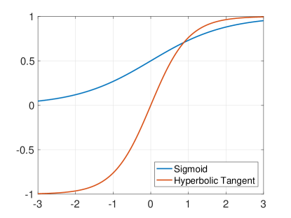
Figure 2: Sigmoid and hyperbolic tangent activation functions.

More practical types of activation functions that are widely used today include the rectified linear unit (ReLU) family.

• ReLU function: $\sigma_{\ell}(x)=\max(0,x)$; see Figure 3 (top).

  This is the most commonly used activation function today. It is cheap and easy to compute and does not cause the vanishing gradient problem. Its (weak) derivative is 0 when $x<0$ and 1 when $x\geq 0$; see the notion of weak derivatives in Chapter 2.

  It also features a property known as “dying ReLU”: since it returns zero for negative inputs, it causes some neurons to remain inactive (or dead). This in turn results in “model sparsity”, which is often desirable. Intuitively, a biological neural network is sparse: among billions of neurons in a human brain, only a portion of them fire (i.e. are active) at a time for a particular task. For example, in a classification problem, there may be a set of neurons that can identify apples, which obviously should not be activated if the image displays a car. But beside the resemblance to biological networks, sparsity in artificial networks have two advantages. First, sparse networks are concise, parsimonious models that often have better predictive power and less overfitting and noise. Second, sparse networks are faster to compute than dense networks, as they involve fewer number of operations.

  The downside of a dying ReLU is that since its slope in the negative range is zero, once a neuron gets negative, it does not learn anything and it may not recover at all, i.e. the neuron may become permanently dead and hence useless. Recall that a single step in SGD involves multiple data points. If for some of them the input to a neuron is not negative, we can still get a slope out of ReLU. The dying problem may also occur when the learning rate is too high, as it would amount to large variations in the weights, turning a positive input into a negative value with a zero ReLU slope.

• Leaky ReLU function: $\sigma_{\ell}(x)=\max(\alpha\,x,x)$, with $\alpha\in(0,1)$ fixed.

  This activation function prevents the dying ReLU problem to some extent: it has a small slope in the negative range. The parameter $\alpha$ is usually set to 0.01-0.05. Note that if we set $\alpha=0$ then we get ReLU, and if we set $\alpha=1$ then we get the identity function; see Figure 3 (middle).

• Parametric ReLU function: $\sigma_{\ell}(x)=\max(\alpha\,x,x)$, with variable parameter $\ \alpha\in(0,1)$.

  It is a type of leaky ReLU, with $\alpha$ being a hyper-parameter, rather than a predetermined fixed value; see Figure 3 (middle).

• ReLU6 function: $\sigma_{\ell}(x)=\min(\max(\alpha\,x,x),6)$.

  This is ReLU restricted on the positive side by value 6. It suppresses very large activations and hence prevents the gradient from blowing up; see Figure 3 (bottom).

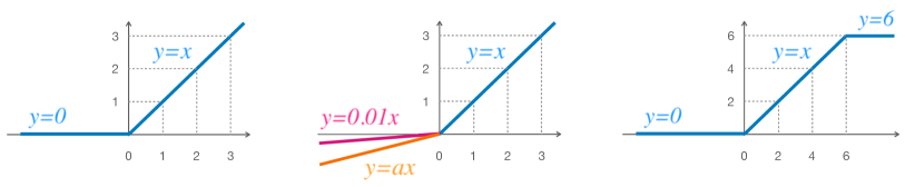
Figure 3: ReLU family of activation functions.

6 Loss functions

Quadratic loss. The quadratic loss function, given in (5),

$$C_{m}(\boldsymbol{\theta})=\frac{1}{2}\,\sum_{j=1}^{n_{\text{out}}}(y_{j}^{(m)}-a_{j}^{L}(\boldsymbol{\theta}))^{2},$$

is a very common loss function in regression problems.

Cross-entropy loss. The cross-entropy (or Kulback-Leibler) loss function is often used in classification problems. Given a set of labeled training data $\{({\bf x}^{(m)},c^{(m)})\}_{m=1}^{n}$ with class labels $c^{(m)}\in\{c_{1},\dotsc,c_{n_{\text{out}}}\}$, the cross-entropy loss function reads

$$C_{m}(\boldsymbol{\theta})=-\,\sum_{j=1}^{n_{\text{out}}}\delta_{m,j}\,\log(a_{j}^{L}(\boldsymbol{\theta})),\qquad a_{j}^{L}=p_{j}=\text{Prob}(c_{j}|{\bf x}^{(m)}),$$ (10)

where

$$\delta_{m,j}=\left\{\begin{array}[]{l l}1&\qquad\text{if}\ \ c^{(m)}=c_{j},\\ 0&\qquad\text{otherwise},\end{array}\right.$$

is a 0-1 binary variable that indicates the “true” distribution of class membership, and $a_{j}^{L}$ is the $j$-th output of the softmax activation function applied to the last layer of the network that indicates the “predicted” distribution. The cross-entropy loss is indeed the Kulbacl-Leibler divergence between the true and predicted distributions. It is easy to see that

$$C_{m}(\boldsymbol{\theta})=-\,\log(\text{Prob}(c^{(m)}|{\bf x}^{(m)})),$$

that is, for each $m$, we find the output index $j$ for which $c_{j}=c^{(m)}$.

We note that adapting the backpropagation algorithm of Section 4.2 to either regressin problems, e.g. with the quadratic loss and identity activation at the last layer, or classification problems, e.g. with the cross-entropy loss and softmax activation at the last layer, will be straightforward, and hence we leave it as an exercise.

7 Overfitting and regularization

The training strategy discussed so far may suffer from overfitting (or overtraining), that is, the trained network ${\bf f}_{\boldsymbol{\theta}}({\bf x})$ may not perform well in approximating ${\bf y}$ outside the set of training data $\{({\bf x}^{(m)},{\bf y}^{(m)})\}_{m=1}^{n}$.

The first step in avoiding overfitting is to detect overfitting. For this purpose, we usually split the available data into two categories: training data and test data. While we train the network using the training data and monitor how the loss on training data changes as the network trains, we also keep track of the loss on the test data. This tells us if and how the trained network generalizes to the test data. Figure 4 shows a case where we observe a decrease in the loss on the training data, meaning that the network fits (or learns) the training data well, while the loss on the test data starts increasing after an initial drop. This is a sign of overfitting and lack of generalization.

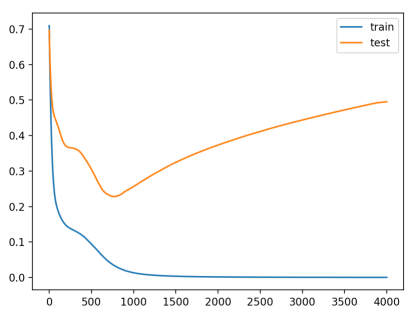
Figure 4: The loss on training data versus test data as the number of epochs increases.

Obviously, increasing the amount of training data is one way of reducing overfitting. Another trivial approach is to reduce the complexity of our network, i.e. to reduce the number of network parameters. Unfortunately, both approaches are not very practical. Often, the number of training data cannot be increased because either they are not available to us or they are very expensive or difficult to obtain. Moreover, networks with larger number of parameters (such as very deep networks) have the potential to be more powerful, and hence reducing complexity of networks may not be a good option; we will discuss the power of “depth” in more details in Chapters 2-3. Fortunately, there are other techniques, known as regularization techniques, that can help reduce overfitting given a fixed number of data points and a fixed number of network parameters. Examples include the addition of a regularization (or penalty) term to the loss function, early stopping, and dropout [28].

7.1 Adding penalty terms

In this approach, we modify the loss function by adding a regularizing (or penalty) term. We consider two types of regularizers, namely $L^{2}$ and $L^{1}$ regularizers.

$L^{2}$ regularizers. A common penalty term is the $L^{2}$-norm of all weights (all parameters excluding biases) scaled by a factor $\lambda$ to the loss function. That is, we consider the $L^{2}$-regularized loss

$$R_{n}(\boldsymbol{\theta})=\frac{1}{n}\sum_{m=1}^{n}C_{m}(\boldsymbol{\theta})+\lambda\,||\boldsymbol{\theta}_{w}||_{2}^{2},$$

where $\boldsymbol{\theta}_{w}$ denotes the vector of all weights excluding biases. The parameter $\lambda>0$ is a hyper-parameter known as the regularization parameter.

The main effect of this regularization term is to learn smaller weights unless large weights substantially reduce the first part of the loss. It introduces a compromise between minimizing the original (non-regularized) loss and finding small wights. The regularization parameter $\lambda$ determines the relative importance of each term: the large $\lambda$, the more emphasize is put on the penalty term.

Why does such regularization help reduce overfitting? In fact, smaller weights amount to smaller fluctuations in the output (more regularized outputs). When weights are small, the network output would not change much if we make small changes in the input. This is analogous to the behavior of simpler models which are more generalizable.

Beside reducing overfitting, smaller weights may help GD/SGD converge faster. When we minimize a non-regularized loss, the size of weights is likely to grow. This may cause the weights moving in pretty much the same direction and hence converging very slowly to the global minimum as GD/SGD makes only small changes to the direction. Another advantage of adding such a penalty term is that it makes the loss function more convex (and hence with less local minima) and the GD/SGD more robust with respect to the initial guess. A non-convex loss with multiple local minima may cause the weights to get stuck in local minima. In this case, the learning process becomes sensitive to the initial guess. An initial guess that is close to a local minima would converge much slower than an initial guess that happen to be close to the global minimum.

It is to be noted that the main reason that biases are excluded in regularization is that large biases would not make the network output sensitive to the input.

$L^{1}$ regularizers. Another penalty term is the $L^{1}$-norm (instead of $L^{2}$ norm), which gives the $L^{1}$-regularized loss,

$$R_{n}(\boldsymbol{\theta})=\frac{1}{n}\sum_{m=1}^{n}C_{m}(\boldsymbol{\theta})+\lambda\,||\boldsymbol{\theta}_{w}||_{1}.$$

Similar to the case of $L^{2}$ regularization, the $L^{1}$-regularized loss penalizes large weights, forcing the network to learn small weights. There is however a difference between the two approaches in the way the weights decrease at each iteration of GD/SGD. To see this, let us consider a single weight, say $w:=W_{j,k}^{\ell}$ for some fixed $j,k,\ell$. Then, a GD update of $w$ reads

$$w^{(k+1)}=w^{(k)}-\eta\,\frac{\partial R_{n}}{\partial w}.$$

With $L^{1}$ regularization, we get

$$w^{(k+1)}=w^{(k)}-\frac{\eta}{n}\sum_{m=1}^{n}\frac{\partial C_{m}}{\partial w}-\eta\,\lambda\,\text{sgn}(w^{(k)}),$$

and with $L^{2}$ regularization, we get

$$w^{(k+1)}=w^{(k)}-\frac{\eta}{n}\sum_{m=1}^{n}\frac{\partial C_{m}}{\partial w}-\eta\,\lambda\,w^{(k)}.$$

In both cases $w$ decreases due to the penalty terms (i.e. the third terms in the right hand side of the above two formulas). However, with $L^{1}$ regularization $w$ decreases by a fixed amount, while with $L^{2}$ regularization $w$ decreases by an amount proportional to $w$. Consequently, when $|w|$ is large, $L^{2}$ regularization reduces the weight much more than $L^{1}$ regularization, and when $|w|$ is small, $L^{2}$ regularization does not reduce it as much as $L^{1}$ does. This amounts to a more balanced distribution of weights in the case of $L^{2}$ regularization (pretty much like averaging), while $L^{1}$ regularization tends to drive some weights toward zero keeping some others of high importance (pretty much like median). Moreover, since $L^{2}$ does not change small weights much, and in particular it does not drive them to zero, it amounts to a dense weight vector (with many non-zeros). However, $L^{1}$ brings sparsity to the weights by making small weights zero.

7.2 Early stopping

In this approach, we split the available data into three categories: training data, test data, and validation data. We will monitor the loss on the validation data (instead of the test loss) at the end of each epoch. Once we are confident that the validation loss does no longer decrease, we stop training; see Section 8 for more details on the validation set.

7.3 Dropout

In this approach, we modify the network and its training process, rather than modifying the loss function. The modification is as follows. Over a mini-batch of data points, we randomly select a portion, usually half, of hidden neurons (i.e. neurons in the hidden layers, excluding input and output layers). We then dropout the selected neurons, that is, we temporarily remove those neurons from the network, along with their incoming and outgoing connections. We perform all forward and backward passes in the mini-batch through the modified network and update the weights and biases corresponding to active neurons. For the next mini-batch, we restore the dropout neurons in the previous mini-batch and randomly select a new set of dropout neurons. We repeat this process: for each mini-batch we select a new set of dropout neurons and update the weights and biases for active neurons. In the end, we have updated the weights and biases of the full network, but always using half the hidden neurons. After training is over, dropout is no longer used when making a prediction with the full network. Since the full network has twice as many active hidden neurons, we halve the weights “outgoing” from hidden neurons. We can think of the network as one in which each hidden neuron is retained during training with a fixed probability $p=0.5$ independent of other neurons. If a neuron is retained with probability $p$ during training, the outgoing weights of that neuron are multiplied by $p$ at the test time. We note that to effectively remove a neuron from a network, we can simply multiply the value of its output weight by zero. This is why only the output weights will be scaled by the selected rate, not biases.

Why would dropout help with regularization? Intuitively, we can think of dropout as a method of training a large number of neural networks with different architectures in parallel. This implies that we have trained multiple models and will be evaluating and averaging multiple models on each test example. Regularization is a direct consequence of averaging. In fact, different models may overfit in different ways, and averaging may help eliminate or reduce overfitting.

8 Validation and hyper-parameter tuning

Each optimization/regularization technique involves a few hyper-parameters, such as learning rates, number of epochs, mini-batch sizes, regularization parameters, dropout rates, and so forth. The hyper-parameters are often tuned using a validation set, i.e. a set of data points that are not directly used in the optimization process. A common practice is to select a large portion of the available set of $n$ data points as training data and a smaller portion of the data as the validation data. Here, we will review a few heuristic strategies for selecting hyper-parameters. We refer to [2, 14] for more details on the subject.

Learning rate $\eta$. Recall that GD/SGD tries to bring us down to the valley of the loss function with steps proportional to $\eta$. If $\eta$ is too large, the steps will also be large, and it is likely that we overshoot the minimum getting to the other side of valley. If $\eta$ is too small, the steps will be very small, and it will slow down the convergence of GD/SGD. Usually, we start with a small value, say $\eta=0.1$, and monitor the training-validation losses for a few epochs. Depending on the behavior of the loss we may need to increase or decrease the value of $\eta$. After we find a “good” value for $\eta$, we can keep it fixed during the training process. However, it is usually better to let $\eta$ vary as we train, following the same strategy as early stopping. That is, we hold the learning rate constant until the validation loss stops decreasing, and then we decrease the learning rate by a factor, say 2-10, and continue this process.

Number of epochs $n_{e}$. We usually use early stopping to determine the number of epochs. At the end of each epoch, we monitor the validation loss. If it stops decreasing after a few epochs, we stop and this automatically determines the number of epochs. Hence, early stopping both prevents overfitting and provides a strategy to automatically take care of the number of epochs and to terminate training.

Regularization parameter $\lambda$. Similar to $\eta$, we first determine a reasonable value for $\lambda$ by training over a few epochs. Then we monitor the validation loss and change and fine-tune $\lambda$ whenever needed.

Mini-batch size $n_{b}$. In general, smaller batch sizes would give a faster GD/SGD convergence, as we update the parameters more often, but at the same time may result in a slower learning, due to a poorer approximation of the sample gradient. There should be a compromise between the speed of learning and convergence. The mini-batch size is relatively independent of other hyper-parameters and mainly affect the speed of learning. Usually, we start with a reasonable set (not necessarily optimal) of other hyper-parameters. Then we use validation data to select a pretty optimal mini-batch size that gives the fastest improvement in performance (i.e. CPU-time). For this purpose we can plot the validation error versus CPU-time (not versus the number of epochs) for several different batch sizes and then select the mini-batch size that gives us the fastest decay in the validation loss. With the mini-batch size fixed, we can proceed to fine-tune other hyper-parameters.

9 Procedure summary

We finally summarize the general procedure:

• Data preparation: We first decide (based on our available budget) about the quantity and quality of data and collect the data. We then split the data into three non-overlapping sets: 1) a training set; 2) a validation set; and 3) a test set. All data sets should be representative of the problem in hand, and the usual size rule is to take the size of training set larger than the size of validation set which is in turn larger in size than the test set. As an example, we may consider a $70\%-20\%-10\%$ split.

• Network architecture: We select the number of layers, neurons, and activation functions for the problem in hand.

• Network training: We use the training set (for computing cost gradients) and the validation set (for hyper-parameter tuning) to learn the network parameters.

• Network evaluation: We use the test set to evaluate (or test) the trained network. If the network passes the test, it is ready to be used for predication.

• Network prediction: The trained network that has passed evaluation can now be used to make predictions.

Chapter Deep neural networks and linear approximation

The goal of this chapter is to review a combination of classical ideas and more recent developments on the approximation theory of deep neural networks within the framework of linear approximation. We will start with an introduction to the concept of density in polynomial approximation and in particular will study the Stone-Weierstrass theorem for real-valued continuous functions. We will continue with a few classical results on the density and convergence rate of two-layer feedforward networks (or perceptrons). We finally discuss more recent developments on the complexity of deep networks in approximating Sobolev functions and by comparing networks with linear approximation methods.

10 Introduction

Let $X\subset{\mathbb{R}}^{d}$ be a compact, convex domain in ${\mathbb{R}}^{d}$. Let $f:X\rightarrow{\mathbb{R}}$ be a real-valued function, referred to as the target function, in some known function space ${\mathcal{F}}(X)$. Two particular examples of ${\mathcal{F}}$ that we will consider include the set of continuous functions, denoted by $C(X)$, and the set of Sobolev functions, denoted by $W^{k,p}(X)$; see the definition of the Sobolev space $W^{k,p}(X)$ in Section 13.2. We say $f$ is a complicated function if its evaluation at any point ${\bf x}\in X$ is computationally expensive, and our computational budget and resources allow only a finite (and often small) number of evaluations of $f$. We therefore wish to approximate the complicated target function $f$ by a simpler approximant being a neural network (NN) $f_{\boldsymbol{\theta}}:{\mathbb{R}}^{d}\rightarrow{\mathbb{R}}$ that has $n_{\boldsymbol{\theta}}$ parameters.

In this context, where the approximant is a neural network, the main task of approximation theory is to study the approximability of the target function by neural networks. Specifically, by such studies we try to address three major questions:

• Density: if $n_{\boldsymbol{\theta}}\rightarrow\infty$, is there $f_{\boldsymbol{\theta}}$ that can approximate $f$ arbitrarily well?

• Convergence rate: if $n_{\boldsymbol{\theta}}<\infty$ fixed, how close can $f_{\boldsymbol{\theta}}$ be to $f$?

• Complexity: if we want $||f-f_{\boldsymbol{\theta}}||<\varepsilon$, how large should $n_{\boldsymbol{\theta}}$ be?

The first question, i.e. the question of density, is a very important one concerning the possibility of approximation: when does $f_{\boldsymbol{\theta}}$ have the theoretical ability to approximate $f$ arbitrarily well? In other words, can we approximate any traget function in the function space as accurately as we wish by a function from the family of neural networks? Or equivalently, is the family of neural networks “dense” in the target function space? For this reason, and in order to better grasp the concept of density, we will start with density in a simpler case where the approximants are algebraic polynomials, rather than neural networks (see Section 11). We then discuss a few classical density results and convergence rates for two-layer feedforward networks (see Sections 12-13). Finally, we study more recent developments on the complexity of deep NNs in Sobolev spaces (see Section 14).

Remark 3.

(An open problem) One important problem that will not be addressed here concerns the selection and preparation of training data $\{({\bf x}^{(i)},f({\bf x}^{(i)}))\}_{i=1}^{n}$. Precisely, to achieve a desired accuracy constraint $||f-f_{\boldsymbol{\theta}}||<\varepsilon$, we would wish to know how to optimally select the number $n$ of data points, the location (or distribution) of support points $\{{\bf x}^{(i)}\}_{i=1}^{n}$ in $X$, and the quality of the output data points, i.e. how accurately to compute $\{f({\bf x}^{(i)})\}_{i=1}^{n}$. This is still an open problem, and we simply assume that we have as many high-quality data points as needed.

Remark 4.

(Approximation theory and numerical analysis) Both approximation theory and numerical analysis are branches of analysis. They share similar goals. In general, more accurate approximations of a target function can be achieved only by increasing the complexity of the approximants. The understanding of such a trade-off between accuracy and complexity is the main goal of “constructive approximation”: how the approximation can be constructed. In this sense, the goals of approximation theory (and in particular constructive approximation) and numerical analysis are similar. Approximation theory is however less concerned with computational issues than numerical analysis. Also, in numerical computation, the target functions are often implicitly available, for instance through differential equations, integral equations, or integro-differential equations. Those interested in the field of approximation theory (not in the context of neural networks) may refer to [30, 25, 9, 8].

11 Density in polynomial approximation

In 1885 Karl Weierstrass, a German mathematician and the “father of modern analysis”, proved that algebraic polynomials are dense in the set of real-valued continuous functions on closed intervals. Later, in 1937 Marshall Stone, an American mathematician, proved the Stone–Weierstrass theorem that generalizes Weierstrass’s theorem on the uniform approximation of continuous functions by polynomials to higher dimensions. Here, we will review the key concepts in such density results.

11.1 Uniform convergence

For studying density (e.g. in the space of continuous functions) we will need to introduce a notion of “distance” that measures the “closeness” of the target function to the approximant. Here, we will consider uniform norms and hence review the notion of uniform convergence. A sequence $\{f_{m}\}_{m=1}^{\infty}$ of functions is said to converge uniformly to a limiting function $f$ on a set $X$ if given any $\varepsilon>0$, there exists a natural number $N$ such taht $|f({\bf x})-f_{m}({\bf x})|<\varepsilon$ for all $m\geq N$ and for all ${\bf x}\in X$, and we write

$$\hskip 42.67912ptf_{m}\rightarrow f\ \ \ \ \text{uniformly}.$$ (11)

An equivalent formulation for uniform convergence can be given in terms of the supremum norm (also called infinity norm or uniform norm). Let the supremum norm of $f$ be

$$||f||_{\infty}:=\sup_{{\bf x}\in X}|f({\bf x})|.$$

Then the uniform convergence (11) is equivalent to

$$||f-f_{m}||_{\infty}\xrightarrow{m\rightarrow\infty}0.$$ (12)

It is to be noted that uniform convergence is stronger than pointwise convergence (defined by $\lim_{m\rightarrow\infty}f_{m}({\bf x})=f({\bf x}),\ \forall{\bf x}\in X$) in the sense that in uniform convergence $N=N(\varepsilon)$ is independent of the point ${\bf x}\in X$. That is, the rate of convergence of $f_{m}({\bf x})$ to $f({\bf x})$ is uniform throughout the domain $X$, independent of where ${\bf x}\in X$ is. On the contrary, pointwise convergence implies that for every point ${\bf x}\in X$ given in advance, there exists $N=N(\varepsilon,{\bf x})$ such that $|f({\bf x})-f_{m}({\bf x})|<\varepsilon$ for all $m\geq N$ and for that particular ${\bf x}$, and we write

$$\hskip 51.21504ptf_{m}\xrightarrow{m\rightarrow\infty}f,\ \ \ \ \ \forall{\bf x}\in X.$$

In other words, uniform convergence implies pointwise convergence, but the converse is not necessarily true. A counter example is $f_{m}(x)=x^{m}$ on $X=[0,1]$; show that while the sequence converges pointwise to $f(x)=0$ when $x\in[0,1)$ and $f(x)=1$ when $x=1$, it does not converge uniformly to $f(x)$ at e.g. $x=(3/4)^{1/m}<1$ when e.g. $\varepsilon=1/2$, because if it converges uniformly, it would converge to the limit (i.e. $f(x)=0$ for $x<0$) and we would get $3/4=|x^{m}-0|<\varepsilon=1/2$ which is a contradiction. Note that in this example the limiting function $f(x)$ is discontinuous, and recall the uniform limit theorem that states if a sequence of a sequence of continuous functions converges uniformly to a limiting function, the limiting function must be continuous as well.

11.2 Weierstrass approximation theorem

Let $C([a,b])$ denote the space of real-valued continuous functions on the closed interval $[a,b]$ on the real line, where $a<b<\infty$. Note that here we have $X=[a,b]\subset{\mathbb{R}}$. The Weierstrass approximation theorem states that the set of real-valued algebraic polynomials on $[a,b]$ is dense in $C([a,b])$ with respect to the supremum norm. That is, given any function $f\in C([a,b])$, there exists a sequence of algebraic polynomials $\{p_{m}\}_{m=1}^{\infty}$ such that $p_{m}\rightarrow f$ uniformly. We say that $f\in C([a,b])$ can be uniformly approximated as accurately as desired by an algebraic polynomial. The precise statement of the theorem follows.

Weierstrass Theorem. Given a function $f\in C[a,b]$ and an arbitrary $\varepsilon>0$, there exists an algebraic polynomial $p$ such that $|f(x)-p(x)|<\varepsilon$ for all $x\in[a,b]$, or equivalently $||f-p||_{\infty}<\varepsilon$.

Proof. A constructive proof of the Weierstrass theorem can be given using Bernstein polynomials; see the next two sub-sections. ∎

We also note that a similar result holds for $2\,\pi$-periodic continuous functions and trigonometric polynomials, also due to Karl Weierstrass. That is, trigonometric polynomials are dense in the class of $2\,\pi$-periodic continuous functions. Recall that the space of algebraic polynomials of degree at most $m$ is $P_{m}=\text{span}\{1,x,\dotsc,x^{m}\}$, while the space of trigonometric polynomials of degree at most $m$ is $T_{m}=\text{span}\{1,\sin x,\cos x\dotsc,\sin mx,\cos mx\}$.

11.3 Bernstein polynomials

A Bernstein polynomial of degree $m$ is a linear combination of Bernstein basis polynomials:

$$B_{m}(x)=\sum_{k=0}^{m}\alpha_{k}\,b_{k,m}(x),$$

where $b_{0,m},\dotsc,b_{m,m}$ are $m+1$ Bernstein basis polynomials of degree $m$,

$$b_{k,m}(x)=\binom{m}{k}\,x^{k}\,(1-x)^{m-k},\qquad x\in[0,1],\qquad k=0,1,\dotsc,m.$$

with the binomial coefficients defined as

$$\binom{m}{k}=\frac{m!}{k!(m-k)!}.$$

Figure 5 displays Bernstein basis polynomials of degree $m=2$ (left) and $m=3$ (right).

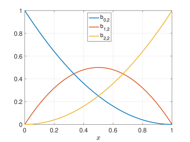
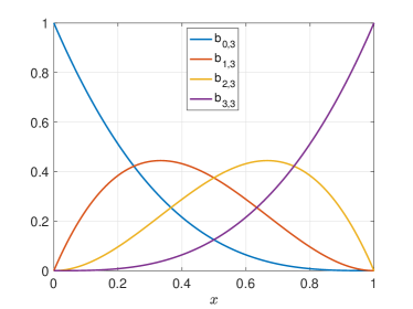
Figure 5: Bernstein basis polynomials of degree $m=2$ (left) and $m=3$ (right).

Bernstein basis polynomials have several interesting properties.

1. Bernstein basis polynomials of degree $m$ form a basis for the vector space $P_{m}$ of polynomials of degree at most $m$ with real coefficients,

   $$P_{m}=\text{span}\{1,x,\dotsc,x^{m}\}=\text{span}\{b_{0,m},b_{1,m},\dotsc,b_{m,m}\},\qquad\forall m\in{\mathbb{N}}_{0}:=\{0,1,2,\dotsc\}.$$

2. Bernstein basis polynomials of degree $m$ form a partition of unity,

   $$\sum_{k=0}^{m}b_{k,m}(x)=1.$$ (13)

   This easily follows from the binomial theorem

   $$(x+y)^{m}=\sum_{k=0}^{m}\binom{m}{k}\,x^{k}\,y^{m-k},$$

   and setting $y=1-x$. However, since the support of all basis functions is the whole interval $[0,1]$, we obtain a partition of unity with a set of functions that are not locally supported on $[0,1]$. That is, at each point $x\in[0,1]$ we cannot find a neighborhood of $x$ where all but a finite number of basis functions in the set are 0.

3. There is an interesting connection between Bernstein basis polynomials and binomial random variables. To illustrate this, fix a point $x\in[0,1]$ and a degree $m$. Consider a random experiment where we carry out a sequence of $m$ independent (Bernoulli) experiments, each with a Boolean-valued outcome: success with probability $x$ and failure with probability $1-x$. Then the probability of observing $k$ successes in $m$ independent Bernoulli trials, denoted by $\text{Pr}(k)$, is given precisely by the Bernstein basis polynomial $b_{k,m}(x)=\binom{m}{k}\,x^{k}\,(1-x)^{m-k}$. In other words, a Bernstein basis polynomial $b_{k,m}(x)$ is the probability mass function of a discrete random variable $k$ that follows a binomial distribution, taking values $0,1,\dotsc,m$.

4. One can show that the expectation and variance of the discrete random variable $\frac{k}{m}$ are given by:

   $${\mathbb{E}}[\,\frac{k}{m}\,]=\sum_{k=0}^{m}\frac{k}{m}\,\text{Pr}(k)=\frac{1}{m}\,\sum_{k=0}^{m}k\,\binom{m}{k}\,x^{k}\,(1-x)^{m-k}=x,$$

   $${\mathbb{V}}[\,\frac{k}{m}\,]={\mathbb{E}}[(\frac{k}{m}-x)^{2}]=\sum_{k=0}^{m}(\frac{k}{m}-x)^{2}\,\binom{m}{k}\,x^{k}\,(1-x)^{m-k}=\frac{x(1-x)}{m}.$$ (14)

   This can be shown either by the binomial theorem or simply by the rules of probability. For instance, let $k\sim B(m,x)$ be a binomially distributed random variable. Noting that $k=k_{1}+\dotsc+k_{m}$ is the sum of $m$ independent Bernoulli random variables each with expected value ${\mathbb{E}}[k_{i}]=x$, $i=1,\dotsc,m$, we can write

   $${\mathbb{E}}[k]={\mathbb{E}}[k_{1}+\dotsc+k_{m}]={\mathbb{E}}[k_{1}]+\dotsc+{\mathbb{E}}[k_{m}]=m\,x.$$

   The formula for variance follows similarly, noting that the variance of the sum of $m$ independent variables is the sum of $m$ variances, each equal to ${\mathbb{V}}[k_{i}]={\mathbb{E}}[k_{i}^{2}]-{\mathbb{E}}[k_{i}]^{2}=x-x^{2}=x(1-x)$, $i=1,\dotsc,m$.

11.4 A constructive proof of Weierstrass theorem

Consider a target function $f\in C([0,1])$. We construct a Bernstein polynomial of degree at most $m$ using a linear combination of Bernstein basis polynomials with coefficients $f(k/m)$:

$$p_{m}(x)=\sum_{k=0}^{m}f(\frac{k}{m})\,b_{k,m}(x).$$

Then by (13), we can write

$$p_{m}(x)-f(x)=\sum_{k=0}^{m}\bigl{(}f(\frac{k}{m})-f(x)\bigr{)}\,b_{k,m}(x).$$

By triangle inequality, we then obtain

$$|p_{m}(x)-f(x)|\leq\sum_{k=0}^{m}\bigl{|}f(\frac{k}{m})-f(x)\bigr{|}\,b_{k,m}(x).$$ (15)

Continuity of $f$ implies that there exists $\delta>0$ such that

$$|f(x_{1})-f(x_{2})|<\varepsilon\quad\text{whenever}\quad|x_{1}-x_{2}|<\delta.$$ (16)

Continuity of $f$ over a bounded set (here the interval $[0,1]$) also implies that the function is bounded, that is,

$$M:=\sup|f|<\infty.$$ (17)

We now split the sum in (15) into two parts and write

$$|p_{m}(x)-f(x)|\leq\sum_{k:\,|x-k/m|<\delta}\bigl{|}f(\frac{k}{m})-f(x)\bigr{|}\,b_{k,m}(x)+\sum_{k:\,|x-k/m|\geq\delta}\bigl{|}f(\frac{k}{m})-f(x)\bigr{|}\,b_{k,m}(x).$$ (18)

The first sum in the right hand side of (18) is bounded by $\varepsilon$, thanks to (13) and (16) (with $x_{1}=x$ and $x_{2}=k/m$). In order to bound the second sum, we note that

$$\bigl{|}f(\frac{k}{m})-f(x)\bigr{|}\leq 2\sup|f|=2\,M.$$

We then write

$$\sum_{k:\,|x-k/m|\geq\delta}\bigl{|}f(\frac{k}{m})-f(x)\bigr{|}\,b_{k,m}(x) \leq 2\,M\sum_{k:\,|x-k/m|\geq\delta}b_{k,m}(x)$$

$$\leq 2\,M\,\sum_{k}\frac{(x-k/m)^{2}}{\delta^{2}}\,b_{k,m}(x)$$

$$=\frac{2\,M}{\delta^{2}}\,\frac{x(1-x)}{m}$$

$$\leq\frac{2\,M}{\delta^{2}\,m},$$

where the equality in the third step above follows from (14), and the inequality in the fourth step follows from $0\leq x(1-x)\leq 1$. We finally obtain

$$|p_{m}(x)-f(x)|\leq\varepsilon+\frac{2\,M}{\delta^{2}\,m}.$$

Hence, since by (17) $M<\infty$, and $\varepsilon>0$ can be selected arbitrarily small, we get $p_{m}\rightarrow f$ uniformly. The proof will be complete by simply extending Bernstein polynomials from $[0,1]$ to $[a,b]$. ∎

11.5 Stone-Weierstrass theorem

Stone generalized and proved the Weierstrass approximation theorem by replacing the closed interval $[a,b]$ by an arbitrary compact Hausdorff space $X$ and considering the space $C(X)$ of real-valued continuous functions on $X$. We note that a Hausdorff space $X$ is a topological space where for every two distinct points $x,y\in X$ there exists a neighborhood $U$ of $x$ and a neighborhood $V$ of $y$ such that $U\cap V=\emptyset$. That is, any two points in $X$ are separated by their neighborhoods that are disjoint. For example, all metric spaces (such as the Euclidean space ${\mathbb{R}}^{d}$) are Hausdorff.

A particular case of Stone-Weierstrass theorem is when $X=[a_{1},b_{1}]\times\dotsc\times[a_{d},b_{d}]\subset{\mathbb{R}}^{d}$. This case can be easily proved by generalizing 1D Bernstein basis polynomials to higher dimensions

$$b_{{\bf k},{\bf m}}({\bf x})=\prod_{i=1}^{d}b_{k_{i},m_{i}}(x_{i})=b_{k_{1},m_{1}}(x_{1})\,\dotsc b_{k_{d},m_{d}}(x_{d}),\qquad{\bf x}=(x_{1},\dotsc,x_{d})\in X,$$

where ${\bf k}=(k_{1},\dotsc,k_{d})$ and ${\bf m}=(m_{1},\dotsc,m_{d})$ are two $d$-dimensional multi-indices.

12 Density of two-layer networks

In this section we will discuss the main density result for two-layer (i.e. shallow) feedforward networks.

12.1 Two-layer feedforward networks

We will consider the family of two-layer feedforward networks with $d$ input neurons, one hidden layer consisting of $r$ neurons, where all $r$ neurons use the same activation function $\sigma:{\mathbb{R}}\rightarrow{\mathbb{R}}$, and one output neuron without any activation function and without any bias. A schematic representation of the network with $d=2$ inputs and $r=3$ neurons in the hidden layer is displayed in Figure 6.

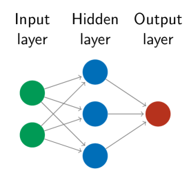
Figure 6: A representation of a feed-forward network with one hidden layer.

Let ${\bf x}=(x_{1},\dotsc,x_{d})\in{\mathbb{R}}^{d}$ be the input variable. Then, the output $y\in{\mathbb{R}}$ of the network can be written as

$$y=\sum_{i=1}^{r}W_{1,i}^{2}\,\sigma(\sum_{j=1}^{d}W_{i,j}^{1}x_{j}+b_{i}),$$

where $W^{1}\in{\mathbb{R}}^{r\times d}$ and $W^{2}\in{\mathbb{R}}^{1\times r}$ are the weight matrices of the two layers, and ${\bf b}=(b_{1},\dotsc,b_{r})\in{\mathbb{R}}^{r}$ is the bias in the hidden layer; see the notation in Chapter 1. Note that there is no output bias here. Setting ${\bf w}^{(i)}:=(W_{i,1}^{1},\dotsc,W_{i,d}^{1})\in{\mathbb{R}}^{d}$, i.e. the $i$-th row of the weight matrix $W^{1}$, and $c_{i}:=W_{1,i}^{2}$, i.e. the $i$-th column of the weight matrix $W^{2}$, we can write the network’s output more succinctly as

$$y=\sum_{i=1}^{r}c_{i}\,\sigma({\bf w}^{(i)}\cdot{\bf x}+b_{i}),$$

where ${\bf a}\cdot{\bf b}:=\sum_{j=1}^{d}a_{j}\,b_{j}$ is the inner product of ${\bf a}\in{\mathbb{R}}^{d}$ and ${\bf b}\in{\mathbb{R}}^{d}$.

12.2 Pinkus theorem

We will consider the density question with such networks. Precisely, we consider the network space (corresponding to the case $r\rightarrow\infty$),

$${\mathcal{M}}(\sigma):=\text{span}\{\sigma({\bf w}\cdot{\bf x}+b)\,:\,{\bf w}\in{\mathbb{R}}^{d},\,b\in{\mathbb{R}}\},$$

and ask for which class of activation functions the network space ${\mathcal{M}}(\sigma)$ is dense in the space $C({\mathbb{R}}^{d})$ of continuous functions with respect to the supremum norm (i.e. in the topology of uniform convergence on compact sets). Equivalently, we would like to know for what $\sigma$, given a target function $f\in C({\mathbb{R}}^{d})$ and a compact subset $X\subset{\mathbb{R}}^{d}$ and an arbitrary $\varepsilon>0$, there exists $g\in{\mathcal{M}}(\sigma)$ such that

$$\sup_{{\bf x}\in X}|f({\bf x})-g({\bf x})|<\varepsilon.$$

Formally, we state the main density result as follows; see Theorem 3.1 in [23].

Pinkus Theorem. Let $\sigma\in C({\mathbb{R}})$. Then ${\mathcal{M}}(\sigma)$ is dense in $C({\mathbb{R}}^{n})$ with respect to the supremum norm on compact sets, if and only if $\sigma$ is not a polynomial.

An intuitive example. Let $d=1$ and assume that $X=[a,b]$ is a closed interval on ${\mathbb{R}}$. Consider a cosine activation function $\sigma(x)=\cos x$, which satisfies the conditions of the above theorem, i.e. it is continuous and not a polynomial. Then $g(x)=\sum_{i\geq 1}c_{i}\,\cos(w_{i}\,x+b_{i})$, which reminds us of Fourier series. In fact this is the so called amplitude-phase form of Fourier series from which we can recover the more familiar sine-cosine form by the identity $\cos(\alpha+\beta)=\cos\alpha\,\cos\beta-\sin\alpha\,\sin\beta$. Recall that if we have a continuous function, we can expand it in Fourier series, and hence it follows that $g$ is dense in the space of continuous functions.

12.3 Proof sketch of Pinkus theorem

First, we need to show that if ${\mathcal{M}}(\sigma)$ is dense, then $\sigma$ is not a polynomial. Suppose $\sigma\in P_{m}({\mathbb{R}})$ is a polynomial of degree $m$, then for every choice of ${\bf w}\in{\mathbb{R}}^{d}$ and $b\in{\mathbb{R}}$, $\sigma({\bf w}\cdot{\bf x}+b)$ is a multivariate polynomial of total degree at most $m$, and thus ${\mathcal{M}}(\sigma)$ is the space of all polynomials of total degree at most $m$, that is ${\mathcal{M}}(\sigma)=P_{m}({\mathbb{R}}^{d})$, which does not span $C({\mathbb{R}}^{d})$, contradicting the density. We next show the converse result: if $\sigma$ is not a polynomial, then ${\mathcal{M}}(\sigma)$ is dense. This is done in four steps:

• Step 1. Consider the 1D case (i.e. $d=1$) and the 1D counterpart of ${\mathcal{M}}(\sigma)$:

  $${\mathcal{N}}(\sigma)=\text{span}\{\sigma(w\,x+b),\,w,b\in{\mathbb{R}}\}.$$

• Step 2. Show that for $\sigma\in C^{\infty}({\mathbb{R}})$ and not a polynomial, ${\mathcal{N}}(\sigma)$ is dense in $C({\mathbb{R}})$.

• Step 3. Weaken the smoothness demand on $\sigma$, using convolution by mollifiers, and show that for $\sigma\in C({\mathbb{R}})$ and not a polynomial, ${\mathcal{N}}(\sigma)$ is dense in $C(\mathbb{R})$.

• Step 4. Extend the result to multiple dimensions: show that if ${\mathcal{N}}(\sigma)$ is dense in $C({\mathbb{R}})$ then ${\mathcal{M}}(\sigma)$ is dense in $C({\mathbb{R}}^{d})$.

Proof of step 2. We will use a very interesting theorem asserting that if a smooth function (i.e. $C^{\infty}$) on an interval is such that its Taylor expansion about every point of the interval has at least one coefficient equal to zero, then the function is a polynomial.

Lemma 1.

Let $\sigma\in C^{\infty}((\alpha,\beta))$, where $(\alpha,\beta)\subset{\mathbb{R}}$ is an open interval on the real line. If for every point $x\in(\alpha,\beta)$ on the interval there exists an integer $k=k(x)$ such that the $k$-th derivative of $\sigma$ vanishes at $x$, i.e. $\sigma^{(k)}(x)=0$, then $\sigma$ is a polynomial.

Proof.

For a proof of this lemma see page 53 in [10]. ∎

Lemma 1 implies that since $\sigma$ is smooth and not a polynomial, there exists a point $b_{0}\in{\mathbb{R}}$ at which $\sigma^{(k)}\neq 0$, $k=0,1,2,\dotsc$. Now we note that

$$\frac{\sigma((w+h)\,x+b_{0})-\sigma(w\,x+b_{0})}{h}\in{\mathcal{N}}(\sigma),\qquad\forall\,h\neq 0,$$

where $w\in{\mathbb{R}}$. Taking the limit (as $h\rightarrow 0$), it follows that the derivative of $\sigma$ with respect to $w$ is in $\overline{{\mathcal{N}}(\sigma)}$, which is the closure of ${\mathcal{N}}(\sigma)$. In particular, for $w=0$ we get

$$\frac{d}{dw}\sigma(w\,x+b_{0})\Big{|}_{w=0}=x\,\sigma^{\prime}(b_{0})\in\overline{{\mathcal{N}}(\sigma)},$$

Similarly (by considering $k+1$ terms of $\sigma$ and taking the limit $h\rightarrow 0$) we can show that

$$\frac{d^{k}}{dw^{k}}\sigma(w\,x+b_{0})\Big{|}_{w=0}=x^{k}\,\sigma^{(k)}(b_{0})\in\overline{{\mathcal{N}}(\sigma)}.$$

Since $\sigma^{(k)}\neq 0$, $k=0,1,2,\dotsc$, the set $\overline{{\mathcal{N}}(\sigma)}$ contains all monomials. By the Weierstrass Theorem this implies that $\overline{{\mathcal{N}}(\sigma)}$ and hence ${\mathcal{N}}(\sigma)$ is dense in $C({\mathbb{R}})$, because if the closure of a function space is dense, the function space will be dense too: we can approximate any function in the closure space by functions in the space as accurately as we wish.

Proof of step 3. The proof utilizes the classical technique of convolution by mollifiers to weaken the smoothness requirement of $\sigma$. In this technique we consider a mollified activation function $\sigma_{\phi}(x)$ obtained by convolving $\sigma\in C({\mathbb{R}})$ with a smooth and compactly supported mollifier $\phi\in C_{0}^{\infty}({\mathbb{R}})$,

$$\sigma_{\phi}(x)=\int_{\mathbb{R}}\sigma(x-y)\,\phi(y)\,dy.$$

Since both $\sigma$ and $\phi$ are continuous and $\phi$ has compact support, the above integral exists for all $x\in{\mathbb{R}}$. We also have $\sigma_{\phi}\in C^{\infty}({\mathbb{R}})$. Moreover, taking the limit of Riemann sums, one can easily show that $\sigma_{\phi}$ and $\overline{{\mathcal{N}}(\sigma_{\phi})}$ are contained in $\overline{{\mathcal{N}}(\sigma)}$. Now since $\sigma_{\phi}\in C^{\infty}({\mathbb{R}})$, provided we choose $\phi$ such that $\sigma_{\phi}$ is not a polynomial (also note that $\sigma$ is not a polynomial), then by the method of proof of Step 2, all monomials are contained in $\overline{{\mathcal{N}}(\sigma_{\phi})}$. Hence $\overline{{\mathcal{N}}(\sigma_{\phi})}$ and therefore $\overline{{\mathcal{N}}(\sigma)}$ and ${\mathcal{N}}(\sigma)$ are dense in $C({\mathbb{R}})$.

Proof of step 4. One interesting technique to “reduce dimension” (here we want to reduce $d$ to 1) is to utilize ridge functions, also known as plane waveforms in the context of hyperbolic PDEs. A ridge function $g:{\mathbb{R}}\rightarrow{\mathbb{R}}$ is a multivariate function $f:{\mathbb{R}}^{d}\rightarrow{\mathbb{R}}$ of the form

$$f({\bf x})=g({\bf w}\cdot{\bf x}),\quad{\bf w}\in{\mathbb{R}}^{d}\setminus\{{\bf 0}\}.$$

Figure 7 displays an example of a ridge function $g({\bf w}\cdot{\bf x})=\sin{\bf w}\cdot{\bf x}$, where ${\bf x}=(x_{1},x_{2})\in{\mathbb{R}}^{2}$, with three choices ${\bf w}=(0,1)$ (left), ${\bf w}=(1,0)$ (middle), and ${\bf w}=(1/\sqrt{2},1/\sqrt{2})$ (right).

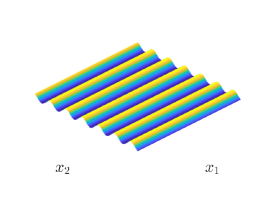
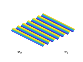
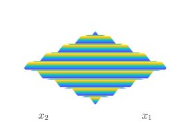
$\sin(0.x_{1}+1.x_{2})$	$\sin(1.x_{1}+0.x_{2})$	$\sin(\frac{1}{\sqrt{2}}.x_{1}+\frac{1}{\sqrt{2}}.x_{2})$

Figure 7: An example of a ridge function $g({\bf w}\cdot{\bf x})=\sin{\bf w}\cdot{\bf x}$ in two dimensions, where ${\bf x}=(x_{1},x_{2})\in{\mathbb{R}}^{2}$, and for three different direction vectors ${\bf w}=(0,1)$ (left), ${\bf w}=(1,0)$ (middle), and ${\bf w}=(1/\sqrt{2},1/\sqrt{2})$ (right).

As we observe, the vector ${\bf w}\in{\mathbb{R}}^{d}\setminus\{{\bf 0}\}$ determines the direction of the plane wave. Importantly, for each ${\bf w}\in{\mathbb{R}}^{d}\setminus\{{\bf 0}\}$ and $b\in{\mathbb{R}}$, the function $\sigma({\bf w}\cdot{\bf x}+b)$ that is the building block of ${\mathcal{M}}(\sigma)$ is also a ridge functions. Now let

$${\mathcal{R}}:=\text{span}\{g({\bf w}\cdot{\bf x}):\,{\bf w}\in{\mathbb{R}}^{d},\,||{\bf w}||_{2}=1,\,g\in C({\mathbb{R}})\}.$$

We first note that ${\mathcal{R}}$ is dense in $C({\mathbb{R}}^{d})$, because it contains all functions of the form $\cos({\bf w}\cdot{\bf x})$ and $\sin({\bf w}\cdot{\bf x})$ which are dense on any compact subset of $C({\mathbb{R}}^{d})$. Of course, this does not directly imply that ${\mathcal{M}}(\sigma)$ will also be dense, because $g$ in ${\mathcal{R}}$ can be any continuous function of ${\bf w}\cdot{\bf x}$, while $\sigma$ is a fixed, given continuous function. However, if ridge functions in ${\mathcal{R}}$ were not dense in $C({\mathbb{R}}^{d})$, then it would not be possible for ${\mathcal{M}}(\sigma)$ to be dense in $C({\mathbb{R}}^{d})$. Now let $f\in C(X)$ be a given target function on some compact set $X\subset{\mathbb{R}}^{d}$. Since ${\mathcal{R}}$ is dense in $C(X)$, then given $\varepsilon>0$ there exist $\{g_{i}\}_{i=1}^{r}\in C({\mathbb{R}})$ and ${\bf w}^{(i)}\in{\mathbb{R}}^{d}$ with $||{\bf w}^{(i)}||_{2}=1$, $i=1,\dotsc,r$ (for some $r$) such that

$$|f({\bf x})-\sum_{i=1}^{r}g_{i}({\bf w}^{(i)}\cdot{\bf x})|<\frac{\varepsilon}{2},\qquad\forall\,{\bf x}\in X.$$

Since $X$ is compact, then for each $i=1,\dotsc,r$, we have $\{{\bf w}^{(i)}\cdot{\bf x}:\,{\bf x}\in X\}\subseteq[a_{i},b_{i}]$ for some bounded interval $[a_{i},b_{i}]$. We next utilize the fact that ${\mathcal{N}}(\sigma)$ is dense in $C([a_{i},b_{i}])$, for all $i=1,\dotsc,r$, which implies that there exist $c_{i,j},\,w_{i,j},\,b_{i,j}\in{\mathbb{R}}$, with $j=1,\dotsc,m_{i}$ for some $m_{i}$, such that

$$|g_{i}(t)-\sum_{j=1}^{m_{i}}c_{i,j}\,\sigma(w_{i,j}\,t+b_{i,j})|<\frac{\varepsilon}{2\,r},\qquad\forall t\in[a_{i},b_{i}],\quad i=1,\dotsc,r.$$

Hence, combining the above two inequalities, we get

$$|f({\bf x})-\sum_{i=1}^{r}\sum_{j=1}^{m_{i}}c_{i,j}\,\sigma(w_{i,j}\,{\bf w}^{(i)}\cdot{\bf x}+b_{i,j})|=$$

$$|f({\bf x})-\sum_{i=1}^{r}g_{i}({\bf w}^{(i)}\cdot{\bf x})+\sum_{i=1}^{r}g_{i}({\bf w}^{(i)}\cdot{\bf x})-\sum_{i=1}^{r}\sum_{j=1}^{m_{i}}c_{i,j}\,\sigma(w_{i,j}\,{\bf w}^{(i)}\cdot{\bf x}+b_{i,j})|\leq$$

$$|f({\bf x})-\sum_{i=1}^{r}g_{i}({\bf w}^{(i)}\cdot{\bf x})|+\sum_{i=1}^{r}|g_{i}({\bf w}^{(i)}\cdot{\bf x})-\sum_{j=1}^{m_{i}}c_{i,j}\,\sigma(w_{i,j}\,{\bf w}^{(i)}\cdot{\bf x}+b_{i,j})|<$$

$$\frac{\varepsilon}{2}+r\,\frac{\varepsilon}{2\,r}=\varepsilon,\qquad\forall\,{\bf x}\in X.$$

Clearly, this implies that there exist $c_{\ell},\,b_{\ell}\in{\mathbb{R}}$ and ${\bf w}^{(\ell)}\in{\mathbb{R}}^{d}$, with $\ell=1,\dotsc,m$ for some $m$, such that

$$|f({\bf x})-\sum_{\ell=1}^{m}c_{\ell}\,\sigma({\bf w}^{(\ell)}\cdot{\bf x}+b_{\ell})|<\varepsilon,\qquad\forall\,{\bf x}\in X.$$

This in turn means that there exist $f_{\boldsymbol{\theta}}\in{\mathcal{M}}(\sigma)$, given by $f_{\boldsymbol{\theta}}({\bf x})=\sum_{\ell=1}^{m}c_{\ell}\,\sigma({\bf w}^{(\ell)}\cdot{\bf x}+b_{\ell})$ for some $m$, such that

$$|f({\bf x})-f_{\boldsymbol{\theta}}({\bf x})|<\varepsilon,\qquad\forall\,{\bf x}\in X.$$

Hence, ${\mathcal{M}}(\sigma)$ is dense in $C(X)$. ∎

13 Convergence rate of approximation by two-layer networks

So far we have discussed the concept of density. We have seen that density addresses only the ability of approximation. It does not tell us anything about the rate of approximation. In particular, density does not imply that one can approximate well by an approximant from the set

$${\mathcal{M}}_{r}(\sigma):=\{\sum_{i=1}^{r}c_{i}\,\sigma({\bf w}^{(i)}\cdot{\bf x}+b_{i}),\,:\,{\bf w}^{(i)}\in{\mathbb{R}}^{d},\,c_{i},b_{i}\in{\mathbb{R}}\},$$

with a fixed $r<\infty$. This is similar to the case of algebraic polynomials: the space of polynomials is dense in $C(X)$, but polynomials of any fixed degree are rather sparse (not dense). In other words, density assumes that the number of parameters in the approximant (such as the number $r$ of neurons and the degree of polynomials) is infinite, and not fixed and finite. When $r$ is fixed and finite, the rate question asks: is there $\gamma>0$ such that

$$\inf_{g\in{\mathcal{M}}_{r}(\sigma)}\sup_{{\bf x}\in X}|f({\bf x})-g({\bf x})|<C\,r^{-\gamma},$$

for some constant $C>0$? Such estimates would tell us the rate (how fast/slow) at which the error converges to zero. The infimum is taken because we want to know the “best” possible convergence rate that can be achieved by the functions in ${\mathcal{M}}_{r}(\sigma)$ (the best case scenario). This question will be discussed in this section for the same family of single hidden-layer feedforward networks considered in Section 12.1.

Of course, similar to density, the rate of approximation has its own limitations. For instance, rate of approximation does not tell us how to find that “best” approximant. It also does not tell us if there are (efficient) methods/algorithms for finding “good” approximants. Nevertheless, it gives us more information than density.

We also note that when $r\rightarrow\infty$, then ${\mathcal{M}}_{r}(\sigma)$ spans the whole ${\mathcal{M}}(\sigma)$. In fact, the density question in terms of the set ${\mathcal{M}}_{r}(\sigma)$ reads: given $f\in C(X)$, is there $g_{r}\in{\mathcal{M}}_{r}(\sigma)$ for which

$$\lim_{r\rightarrow\infty}\sup_{{\bf x}\in X}|f({\bf x})-g_{r}({\bf x})|=0.$$

Clearly, this question does not address the convergence rate of approximation.

Finally, we note that the set ${\mathcal{M}}_{r}$ has the property

$${\mathcal{M}}_{r_{1}}+{\mathcal{M}}_{r_{2}}={\mathcal{M}}_{r_{1}+r_{2}},$$

where the sumset is defined as ${\mathcal{M}}_{r_{1}}+{\mathcal{M}}_{r_{2}}:=\{g_{1}+g_{2}:\ g_{1}\in{\mathcal{M}}_{r_{1}},\,g_{2}\in{\mathcal{M}}_{r_{2}}\}$. This property will be used later to prove the main convergence result. The reason for this property is that ${\mathcal{M}}_{r_{1}}$ and ${\mathcal{M}}_{r_{2}}$ do not necessarily share basis functions $\sigma({\bf w}^{(i)}\cdot{\bf x}+b_{i})$ with the very same $({\bf w}^{(i)},b_{i})$ parameters. In general we have ${\mathcal{M}}_{r_{1}}=\text{span}\{\sigma({\bf w}^{(i)}\cdot{\bf x}+b_{i})\}_{i=1}^{r_{1}}$ and ${\mathcal{M}}_{r_{2}}=\text{span}\{\sigma({\bf w}^{(i)}\cdot{\bf x}+b_{i})\}_{i=r_{1}+1}^{r_{1}+r_{2}}$. In other words, the space ${\mathcal{M}}_{r}$ is a nonlinear space. Note that this will make the neural networks in our setup nonlinear methods of approximation.

13.1 Target functions of interest

Throughout Section 13 we let the domain $X$ be the unit ball

$$X:=\{{\bf x}:\,||{\bf x}||_{2}\leq 1\}\subset{\mathbb{R}}^{d},\qquad d\geq 2.$$

Moreover, instead of continuous target functions that we considered earlier, we will consider Sobolev target functions (see the definition of Sobolev function spaces in Section 13.2),

$$f\in W^{k,p}(X),\qquad k\geq 1,\qquad 1\leq p\leq\infty,\qquad||f||_{W^{k,p}(X)}\leq 1.$$

A major importance of Sobolev functions is that they often appear in the study of PDEs. We want to study the rate of approximation of $f\in W^{k,p}(X)$ by $g\in{\mathcal{M}}_{r}(\sigma)$ with fixed $r<\infty$.

13.2 Sobolev spaces

Here we will briefly review Sobolev spaces. For a more detailed discussion see Sec. 5 in [13].

Strong derivatives. Suppose $f\in C^{k}(X)$, for some non-negative integer $k$. Denote by $\alpha=(\alpha_{1},\dotsc,\alpha_{d})$ a multi-index of $d$ non-negative integers of order $|\alpha|=\alpha_{1}+\dotsc+\alpha_{d}\leq k$. The (strong) $\alpha$-th partial derivative of $f$ is defined as

$$D^{\alpha}f({\bf x}):=\frac{\partial^{|\alpha|}f({\bf x})}{\partial x_{1}^{\alpha_{1}}\dotsc\partial x_{n}^{\alpha_{n}}}=\partial_{x_{1}}^{\alpha_{1}}\dotsc\partial_{x_{n}}^{\alpha_{n}}f({\bf x}),\qquad{\bf x}\in X.$$

Moreover, for every test function $\phi\in C_{0}^{\infty}(X)$, the following integration by parts formula holds

$$\int_{X}f\,D^{\alpha}\phi\,d{\bf x}=(-1)^{|\alpha|}\int_{X}D^{\alpha}f\,\phi\,d{\bf x}.$$

Note that there is no boundary terms involved in the above formula because tests functions have compact support on $X$, and hence all boundary terms vanish.

Weak derivatives. Sometimes (actually often), for example in the context of PDEs, we need to deal with functions $f$ that have low regularity/smoothness. For instance, they may not belong to $C^{k}(X)$, i.e. they are not $k$-times continuously differentiable and hence $D^{\alpha}f({\bf x})$ would not exist in the above sense. For such functions we use a “weaker” notion of derivatives utilizing the integration by parts formula. Precisely, suppose $f\in L^{1}(X)$ (this is why we assume $p\geq 1$). We say that $u$ is the weak $\alpha$-th partial derivative of $f$ provided for all test functions $\phi\in C_{0}^{\infty}(X)$ the following holds

$$\int_{X}f\,D^{\alpha}\phi\,d{\bf x}=(-1)^{|\alpha|}\int_{X}u\,\phi\,d{\bf x}.$$

In this case, we often use the same notation as in the case of strong derivatives and write

$$D^{\alpha}f=u,$$

and say $D^{\alpha}f$ is the $\alpha$-th partial derivative of $f$ in the weak sense.

As an example, it is easy to see that the weak derivative of the ReLU activation function $\sigma(x)=\max\{0,x\}$ on $X=[-1,1]$ is given by

$$u(x)=\left\{\begin{array}[]{l l}0&\qquad-1\leq x<0,\\ 1&\qquad 0\leq x\leq 1.\end{array}\right.$$

Definition of Sobolev spaces. Fix $1\leq p\leq\infty$, and let $k$ be a nonnegative integer. The Sobolev space $W^{k,p}(X)$ consists of all functions $f\in L^{1}(X)$ for which the derivatives $D^{\alpha}f$ for all $\alpha$ with $|\alpha|\leq k$ exist in the weak sense and belong to $L^{p}(X)$. We write

$$W^{k,p}(X):=\{f:X\rightarrow{\mathbb{R}};\,D^{\alpha}f\in L^{p}(X),\,|\alpha|\leq k\},$$

where we understand $D^{\alpha}f$ in the weak sense. In the particular case when $p=2$, we usually use the letter $H$ and omit $p=2$, and write

$$H^{k}(X):=W^{k,2}(X),$$

which is a Hilbert space. Obviously, $H^{0}(X)=W^{0,2}(X)=L^{2}(X)$, which is the space of square-integrable functions on $X$.

Remark 5.

Recall that the $L^{p}$ space (sometimes called Lebesgue space) is defined as

$$L^{p}(X):=\{f:X\rightarrow{\mathbb{R}};\,||f||_{L^{p}(X)}<\infty\},$$

where

$$||f||_{L^{p}(X)}:=\bigl{(}\int_{X}|f|^{p}\,d{\bf x}\bigr{)}^{1/p},\qquad 1\leq p<\infty,$$

and

$$||f||_{L^{\infty}(X)}:=\text{ess}\,\text{sup}_{X}|f|:=\inf\{v\in{\mathbb{R}}|\ \mu(\{x\in X:|f|>v\})=0\}.$$

Here, for any subset $A\subset X$ in ${\mathbb{R}}^{d}$, $\mu(A)$ denotes the $d$-dimensional Lebesgue measure of $A$, which determines the size or $d$-dimensional volume of the subset $A$. Informally, $||f||_{L^{\infty}(X)}$ is the “almost everywhere” supremum of $|f|$ over $X$, that is, the supremum of $|f|$ everywhere on $X$ except on a set of measure zero.

Definition of Sobolev norm. If $f\in W^{k,p}(X)$, we define its norm as

$$||f||_{W^{k,p}(X)}:=\bigl{(}\sum_{|\alpha|\leq k}||D^{\alpha}f||_{L^{p}(X)}^{p}\bigr{)}^{1/p},\qquad 1\leq p<\infty,$$

and

$$||f||_{W^{k,\infty}(X)}:=\sum_{|\alpha|\leq k}||D^{\alpha}f||_{L^{\infty}(X)}.$$

13.3 A typical convergence rate result

Error of interest. To study the convergence rate, we will first need to define an error that we call the error of interest. We will consider the following error

$$\sup_{f\in W^{k,p}(X)}\,\inf_{g\in{\mathcal{M}}_{r}(\sigma)}||f-g||_{L^{p}(X)}.$$

Clearly $W^{k,p}$ is a subspace of $L^{p}$. Moreover, since $X$ is compact and $C(X)$ is dense in $L^{p}(X)$, then by the density result in Section 12, ${\mathcal{M}}_{r}(\sigma)$ will also be dense in $L^{p}(X)$ for each $\sigma\in C({\mathbb{R}})$ that is not a polynomial. Hence, the $L^{p}$ space contains both $W^{k,p}$ and ${\mathcal{M}}_{r}(\sigma)$, and therefore $||f-g||_{L^{p}(X)}$ in the above error is well defined. The infimum over $g\in{\mathcal{M}}_{r}(\sigma)$ is taken because fixing $f$ we want to know how close the space ${\mathcal{M}}_{r}(\sigma)$ can be to $f$ (best case scenario). The supremum over $f\in W^{k,p}(X)$ is taken because we want to consider the worst function $f$ to be approximated (worst case scenario).

A Convergence Theorem. (Theorem 6.8 in [23]; also see Theorem 2.1 in [21]) Let $\sigma\in C^{\infty}(I)$ be a smooth function on some open interval $I\subseteq{\mathbb{R}}$, and suppose that it is not a polynomial on $I$. Then, for each $p\in[1,\infty]$, $k\geq 1$, and $d\geq 2$, there is a constant $C>0$ independent of $r$ such that

$$\sup_{f\in W^{k,p}(X)}\,\inf_{g\in{\mathcal{M}}_{r}(\sigma)}||f-g||_{L^{p}(X)}\leq C\,r^{-k/d}.$$

Remark 6.

Note that, as stated above, we are also assuming that $||f||_{W^{k,p}(X)}\leq 1$. In the general case when the norm of $f$ is bounded by another finite number, e.g. $||f||_{W^{k,p}(X)}\leq a<\infty$, the constant $C$ may also depend on $a$ (i.e. the size of $f$). See Section 14 for this more general case.

The proof of convergence theorem utilizes homogeneous polynomials, and hence here we quickly review them.

Homogeneous polynomials. A homogeneous polynomial of degree $m$ in $d\geq 2$ variables in ${\mathbb{R}}^{d}$ is a polynomial whose non-zero terms all have the same degree $m$. For example, $x_{1}^{5}-2\,x_{1}^{3}\,x_{2}^{2}+x_{1}\,x_{2}^{4}$ is a homogeneous polynomial of degree $m=5$ in two variables with $d=2$. Let us denote by $Q_{m}$ the linear space of such polynomials, i.e. the set of all terms ${\bf x}^{\alpha}:=\prod_{i=1}^{d}x_{i}^{{\alpha}_{i}}$ such that $|\alpha|=\alpha_{1}+\dotsc+\alpha_{d}=m$. A few interesting properties of homogeneous polynomials relevant to our convergence problem follows.

1. The dimension of $Q_{m}$ is the maximal number of non-zero terms ${\bf x}^{\alpha}$ with $|\alpha|=m$, or equivalently the cardinality of the set $\{\alpha=(\alpha_{1},\dotsc,\alpha_{d}):\,|\alpha|=m\}$, which is

   $$s:=\text{dim}\,Q_{m}=\binom{m+d-1}{m}\leq C\,m^{d-1},$$

   where $C=C(d)$ is a constant that may depend only on $d$. The binomial formula can easily be shown by the method of stars and bars, which is a well-known technique in combinatorics. We skip its interesting proof here. The inequality is a simple consequence of $\binom{m+d-1}{m}\leq\bigl{(}\frac{e\,(m+d-1)}{d-1}\bigr{)}^{d-1}$ and $(a+b)^{d-1}\leq 2^{d-2}\,(a^{d-1}+b^{d-1})$, for $d\geq 2$.

2. For a ${\bf w}\in{\mathbb{R}}^{d}$ with unit norm $||{\bf w}||_{2}=1$, we have $({\bf w}\cdot{\bf x})^{m}\in Q_{m}$. This can easily be seen by the multinomial theorem (which is a generalization of the binomial theorem),

   $$(x_{1}+\dotsc+x_{d})^{m}=\sum_{|\alpha|=m}\binom{m}{\alpha}\,{\bf x}^{\alpha},\qquad\binom{m}{\alpha}:=\frac{m!}{\prod_{i=1}^{d}\alpha_{i}!},\qquad{\bf x}^{\alpha}:=\prod_{i=1}^{d}x_{i}^{\alpha_{i}}.$$

3. Consequently, there exist $s=\text{dim}\,Q_{m}$ points ${\bf w}^{(i)}\in{\mathbb{R}}^{d}$ with $||{\bf w}^{(i)}||_{2}=1$, $i=1,\dotsc,s$, such taht $\{({\bf w}^{(i)}\cdot{\bf x})^{m}\}_{i=1}^{s}$ spans $Q_{m}$. This in particular implies that

   $$Q_{\ell}=\text{span}\{({\bf w}^{(i)}\cdot{\bf x})^{\ell}:\,i=1,\dotsc,s\},\qquad\ell=0,1,\dotsc,m.$$

   Hence, for the linear space $P_{m}$ of multivariate polynomials of degree at most $m$,

   $$P_{m}=\cup_{\ell=0}^{m}Q_{\ell},$$

   we have

   $$P_{m}=\text{span}\{({\bf w}^{(i)}\cdot{\bf x})^{\ell}:\,i=1,\dotsc,s,\,\ell=0,1,\dotsc,m\}.$$

   This last formula can aslo be written as

   $$P_{m}=\{\sum_{i=1}^{s}p_{i}({\bf w}^{(i)}\cdot{\bf x}):\ p_{i}\in\pi_{m},\,i=1,\dotsc,s\},$$

   where $\pi_{m}$ denotes the linear space of univariate polynomials of degree at most $m$.

Proof Sketch of Convergence Theorem. Let $Q_{\ell}$ denote the linear space of homogeneous polynomials of degree ${\ell}$ in ${\mathbb{R}}^{d}$, and let $P_{m}:=\cup_{\ell=0}^{m}Q_{\ell}$ be the linear space of multivariate polynomials of degree at most $m$. By the third property of Homogeneous polynomials discussed above, there exists $s=\text{dim}\,Q_{m}$ points ${\bf w}^{(1)},\dotsc,{\bf w}^{(s)}\in{\mathbb{R}}^{d}$ with $||{\bf w}^{(i)}||_{2}=1$, $i=1,\dotsc,s$, such that

$$P_{m}=\{\sum_{i=1}^{s}p_{i}({\bf w}^{(i)}\cdot{\bf x}):\ p_{i}\in\pi_{m},\,i=1,\dotsc,s\},$$

where $\pi_{m}$ denotes the linear space of univariate algebraic polynomials of degree at most $m$. Now, if we consider the 1D counterpart of ${\mathcal{M}}_{r}(\sigma)$:

$${\mathcal{N}}_{r}(\sigma)=\{\sum_{i=1}^{r}c_{i}\,\sigma(w_{i}\,x-b_{i}),\,c_{i},w_{i},b_{i}\in{\mathbb{R}}\},$$

by the method of proof of step 2 in Section 12.3, under the conditions stated in the above theorem, $\overline{{\mathcal{N}}_{m+1}(\sigma)}$, which is the closure of ${\mathcal{N}}_{m+1}(\sigma)$, contains the space $\pi_{m}$ of univariate algebraic polynomials of degree at most $m$. Note that in this method to show a monomial of degree up to $m$ is in the network space, we will need up to the $m$-th derivative of $\sigma$. Using divided differences, this would need a linear combination of $m+1$ terms (e.g. we need 2 terms for first derivative, three terms for second derivative, etc.), and this amounts to a network space ${\mathcal{N}}_{m+1}(\sigma)$ with $m+1$ basis functions. Now from $p_{i}\in\pi_{m}$, it follows that $p_{i}\in\overline{{\mathcal{N}}_{m+1}(\sigma)}$. Hence, using the property ${\mathcal{M}}_{r_{1}}+{\mathcal{M}}_{r_{2}}={\mathcal{M}}_{r_{1}+r_{2}}$, we obtain

$$P_{m}\subseteq\overline{{\mathcal{M}}_{s\,(m+1)}(\sigma)}.$$

By setting $r=s\,(m+1)$, where $s=\text{dim}\,Q_{m}$, we get $P_{m}\subseteq\overline{{\mathcal{M}}_{r}(\sigma)}$, which implies

$$\sup_{f\in W^{k,p}(X)}\,\inf_{g\in{\mathcal{M}}_{r}(\sigma)}||f-g||_{L^{p}(X)} =\sup_{f\in W^{k,p}(X)}\,\inf_{g\in\overline{{\mathcal{M}}_{r}(\sigma)}}||f-g||_{L^{p}(X)}$$

$$\leq\sup_{f\in W^{k,p}(X)}\,\inf_{g\in P_{m}}||f-g||_{L^{p}(X)}.$$

It is also well known (see e.g. Section 5 in [6]) that for every $f\in W^{k,p}(X)$, there exists a polynomial $g\in P_{m}$ such that

$$||f-g||_{L^{p}(X)}\leq C\,m^{-k}\,||f||_{W^{k,p}(X)}.$$

Noting $||f||_{W^{k,p}(X)}\leq 1$, this implies that

$$\sup_{f\in W^{k,p}(X)}\,\inf_{g\in P_{m}}||f-g||_{L^{p}(X)}\leq C\,m^{-k}.$$

The desired estimate then follows noting that $s=\text{dim}\,Q_{m}\leq C(d)\,m^{d-1}$. ∎

13.4 A short discussion on curse of dimension

Suppose that we want to construct an approximation $g\in{\mathcal{M}}_{r}(\sigma)$ of a target function $f\in W^{k,p}$ with an error at most $\varepsilon>0$. Suppose further that the approximation error is proportional to $r^{-k/d}$, as the above theorem suggests. This means that we need $r={\mathcal{O}}(\varepsilon^{-d/k})$ neurons, which demonstrates the curse of dimension: the computational cost (encoded in $r$) increases exponentially with the dimension $d$.

One of the main reasons for current interest in deep neural networks is their outstanding performance in high-dimensional problems, i.e. when $d$ is large. However, the convergence rate ${\mathcal{O}}(r^{-k/d})$ in the theorem in Section 13.3 depends strongly on the dimension $d$ of the input space. Indeed, the theorem suggests that the rate of approximation from ${\mathcal{M}}_{r}(\sigma)$ with $r\sim m^{d}$ (note: $r=s(m+1)\sim m^{d}$) may not be better than the rate of polynomial approximation from the polynomial space $P_{m}$ (which is $\sim m^{-k}$). This makes one wonder whether it is really worthwhile using neural networks (at least in the case of a single hidden layer). One may think that the upper bound in the above theorem may not be sharp. However, there are lower bounds that confirm this is not the case; see e.g. [21, 23, 18]. For instance, with $\sigma(x)=1/(1+\exp(-x))$ being the logistic sigmoid (which in particular satisfies the conditions of the theorem in Section 13.3), we get [18]

$$\sup_{f\in W^{k,p}(X)}\,\inf_{g\in{\mathcal{M}}_{r}(\sigma)}||f-g||_{L^{p}(X)}\geq C\,(r\,\log r)^{-k/d}.$$

Therefore, we cannot expect to circumvent the curse of dimension, at least in the setting considered here.

An interesting approach to obtaining the rate of approximation from the set ${\mathcal{M}}_{r}(\sigma)$ was initiated by Barron [1] and generalized by Makovoz [19]. Barron (and later Makovoz) started with a given ${\mathcal{M}}_{r}(\sigma)$, with a bounded sigmoidal $\sigma$, and tried to find classes of functions which are well approximated by ${\mathcal{M}}_{r}(\sigma)$ with minimal dependence on the dimension $d$. Without going into details, here, we summarize their results.

Barron-Makovoz Theorem. Let ${\mathcal{B}}(X)$ be the set of all functions $f:{\mathbb{R}}^{d}\rightarrow{\mathbb{R}}$ defined on the unit ball $X\subset{\mathbb{R}}^{d}$ that can be extended to all of ${\mathbb{R}}^{d}$ such that some shift of $f$ by a constant has a Fourier transform $\hat{f}$ satisfying $\int_{{\mathbb{R}}^{d}}||\boldsymbol{\xi}||_{2}\,|\hat{f}(\boldsymbol{\xi})|\,d\boldsymbol{\xi}\leq\gamma$ for some $0<\gamma<\infty$, where $||\boldsymbol{\xi}||_{2}=(\boldsymbol{\xi}\cdot\boldsymbol{\xi})^{1/2}$. Then for any bounded sigmoidal function $\sigma$,

$$\sup_{f\in{\mathcal{B}}(X)}\,\inf_{g\in{\mathcal{M}}_{r}(\sigma)}||f-g||_{L^{2}(X)}\leq C\,r^{-(d+1)/2d},$$

where the constant $C>0$ is independent of $r$.

It is to be noted that this result cannot be quite compared to the results of Section 13.3, because, unlike in the case of the Sobolev space $W^{k,p}$, the condition defining the function set ${\mathcal{B}}$, known as Barron space, cannot be restated in terms of the number of derivatives. Nevertheless, Barron has shown that on the unit ball $X$ the following embeddings hold:

$$W^{\lfloor d/2\rfloor+2,\infty}(X)\subseteq\text{span}\,{\mathcal{B}}(X)\subseteq W^{1,\infty}(X).$$

In particular, it tells us that functions $f$ with sufficiently high orders $k=\lfloor d/2\rfloor+2$ of derivatives are in the set ${\mathcal{B}}$. In other words, and roughly speaking, in order to achieve a rate ${\mathcal{O}}(r^{-(d+1)/2d})$ that is almost independent of the dimension $d$ when $d$ is large, the function $f$ would need to have many ($k=\lfloor d/2\rfloor+2$) derivatives. Putting this in the main result of Section 13.3 we would obtain a comprable rate ${\mathcal{O}}(r^{-k/d})={\mathcal{O}}(r^{-(d+4)/2d})$. This in turn implies that in such smooth function spaces with a large number of derivatives available, then both ReLU networks with one hidden layer and polynomials achieve a rate that minimally depends on the dimension (i.e. $-(d+4)/2d$ which approaches $-1/2$ in the limit).

Remark 7.

The original estimate of Barron [1] was (mistakenly) of the form $C\,r^{-1/2}$. This initiated an unfortunate discussion (and misconception) that Barron’s results have broken the curse of dimension.

We close this discussion by pointing out that other network architectures, such as deep convolutional neural network-type architectures that are invariant by construction and serve as the state-of-the-art architectures for image/text/graph-related tasks, may perform better in alleviating the curse of dimension when target functions have certain and a priori known hierarchical/geometric properties. Examples include target functions that have hierarchically local compositional structures, target functions that are invariant to transformations (i.e. translations, permutations, rotations), and target functions that possess geometric stability (or near invariance, smoothness) to small deformations. We refer to [20, 24, 3] and the references therein for further details on the subject.

14 Complexity of deep ReLU networks

So far we have been discussing the density and convergence rate questions regarding the approximation of continuous and Sobolev target functions by feedforward neural networks with one single hidden layer and continuous or smooth non-polynomial activation functions. In the remainder of this chapter we will consider the more practical case of “deep” feedforward networks with “ReLU” activation functions and obtain an estimate of the complexity of the network (i.e. number of layers, neurons, and non-zero parameters) needed for approximating Sobolev target functions within a desired small tolerance $\varepsilon\in(0,1/2)$. We closely follow [31] and [15] in the sense that we utilize the basic element used in those two references: the “sawthooth” construction developed in [29]. Nevertheless, we will present some new results (that are more general than the results in [31] and [15]) with a few changes in the proofs presented in those two references. Other relevant references will be cited in the text whenever an idea/formula/concept is used.

14.1 Target functions of interest

On the unit hypercube domain

$$X=[0,1]^{d}\subset{\mathbb{R}}^{d},$$

we consider Sobolev target functions (see Section 13.2)

$$f\in W^{k,p}(X),\qquad k\geq 1,\qquad 1\leq p\leq\infty.$$

Unlike in [31, 15], we do not assume $||f||_{W^{k,p}(X)}\leq 1$ and will derive more general estimates, i.e. estimates that also depend on $||f||_{W^{k,p}(X)}<\infty$.

14.2 Main complexity result

Complexity Theorem. Let $\varepsilon\in(0,1/2)$. Consider a Sobolev target function $f\in W^{k,p}(X)$ on $X:=[0,1]^{d}$ with $k\geq 1$ and $p\in[1,\infty]$. Then, there exists a standard ReLU neural network $\Phi_{\varepsilon}$ (see definition in Section 14.8) with $d$ inputs and one output and complexity

$$L(\Phi_{\varepsilon})\leq C(d,k,p)\,\log_{2}(\varepsilon^{-1}\,||f||_{W^{k-1,p}(X)}),$$

$$N(\Phi_{\varepsilon}),\,P(\Phi_{\varepsilon})\leq C(d,k,p)\,\varepsilon^{-d/k}\,||f||_{W^{k,p}(X)}^{d/k}\,\log_{2}^{2}(\varepsilon^{-1}\,||f||_{W^{k-1,p}(X)}),$$

such that

$$||f-\Phi_{\varepsilon}||_{L^{p}(X)}\leq\varepsilon.$$

Here, $L,N,P$ denote the number of layers, neurons, and non-zero parameters of the network, respectively, and the constant $C=C(d,k,p)>0$ is independent of $\varepsilon$.

14.3 Proof strategy

The general strategy is to first build a polynomial approximation of $f$ and then approximate the polynomial by a ReLU network, according to the following steps:

1. Part 1: build a polynomial approximation of $f$:

   • Discretize $X=[0,1]^{d}$ into a uniform grid of $(n+1)^{d}$ grid points.

   • Construct a partition of unity as the collection of $(n+1)^{d}$ functions, where each function is supported around a grid point and is the product of $d$ piecewise linear univariate functions (that can be represented by ReLU networks).

   • Around each grid point build a localized polynomial approximation of $f$ by averaged Taylor polynomials (see Section 14.4 for a short introduction to averaged Taylor polynomials).

   • Build a global polynomial approximation of $f$ using the local polynomials and partition of unity constructed in the previous two steps.

2. Part 2: Approximate the global polynomial by a ReLU network:

   • Using the sawtooth function approximate $x^{2}$ by a ReLU network.

   • Utilizing $xy=\frac{1}{2}((x+y)^{2}-x^{2}-y^{2})$, approximate $xy$ by a ReLU network.

   • Construct a ReLU network with $d$ outputs such that the product of its outputs is a function in the partition of unity.

   • Construct a ReLU network such that the product of its outputs expresses each term in the global polynomial.

   • Approximate the products of the outputs of a ReLU network by a ReLU network with one output.

   • Construct the final ReLU network by a linear combination of the one-output networks constructed in the previous step.

   • Estimate the error in approximating the global polynomial by the constructed ReLU network.

3. Part 3: Finally, select the number $n$ of grid points such that the total error (i.e. the sum of errors made in parts 1 and 2) remains below $\varepsilon$ and compute the network complexity.

The remainder of this section will be devoted to the details of the proof. Part 1 will be covered in Sections 14.4-14.6. Part 2 will be discussed through Sections 14.7-14.12. Finally, Part 3 will be done in Section 14.13. Some very recent directions of research on the topic with further reading suggestions will be provided in Section 14.14.

14.4 Averaged Taylor polynomial approximation

We will review an averaged version of the Taylor polynomial of calculus. Averaged Taylor polynomials are particularly suitable for approximating Sobolev functions. A good reference on the topic is Chapter 4 of [5].

Consider a Sobolev function $f\in W^{k,p}(X)$, where $X\subset{\mathbb{R}}^{d}$ is a bounded convex domain. Let

$$B:=B({\bf x}_{0},r)=\{{\bf x}\in X:||{\bf x}-{\bf x}_{0}||_{2}<r\},$$

be the open ball centered at ${\bf x}_{0}\in X$ with radius $r>0$ such that $B\subset X$. Consider a cut-off function $\phi\in C_{0}^{\infty}({\mathbb{R}}^{d})$ with the properties

$$\phi\geq 0,\qquad\text{supp}\,\phi=\overline{B},\qquad\int_{{\mathbb{R}}^{d}}\phi({\bf x})\,d{\bf x}=1.$$

The Taylor polynomial of order $k$ of $f$ averaged over $B$ is defined as

$$Q^{k}f({\bf x}):=\int_{B}T_{\bf y}^{k}f({\bf x})\,\phi({\bf y})\,d{\bf y},\qquad{\bf x}\in X,$$

where $T_{\bf y}^{k}f({\bf x})$ is the familiar Taylor polynomial of order $k-1$ about ${\bf y}$:

$$T_{\bf y}^{k}f({\bf x}):=\sum_{|\boldsymbol{\alpha}|\leq k-1}\frac{1}{\boldsymbol{\alpha}!}\,D^{\boldsymbol{\alpha}}f({\bf y})\,({\bf x}-{\bf y})^{\boldsymbol{\alpha}}.$$

Here, we have used the standard multi-index notation for the multi-index $\boldsymbol{\alpha}=(\alpha_{1},\dotsc,\alpha_{d})$. Note that since $f\in W^{k,p}(X)$ with $k\geq 1$, then $f\in W^{k-1,p}(X)$ and $D^{\boldsymbol{\alpha}}f$ with $|\boldsymbol{\alpha}|\leq k-1$ is bounded.

Remark 8.

(Why do we use averaged Taylor polynomials for Sobolev functions?) In general, for a Sobolev function $f$, the derivatives $D^{\boldsymbol{\alpha}}f$ that appear in Taylor’s formula may not exist in the usual pointwise (or strong) sense. One possibility to define a Taylor polynomial for such a function is by taking a smoothed average of $T_{\bf y}^{k}f({\bf x})$ over ${\bf y}\in B$.

A few properties of averaged Taylor polynomials (without proofs) follow.

Linearity property. From the linearity of weak derivatives, we can conclude that averaged Taylor polynomials are linear in $f$.

Polynomial property. Let $f\in W^{k,p}(X)$, where $X\subset{\mathbb{R}}^{d}$ is a bounded convex domain. The Taylor polynomial of order $k$ of $f$ averaged over a ball $B\subset X$ is a polynomial of degree less than $k$ in x that can be written as

$$Q^{k}f({\bf x})=\sum_{|\boldsymbol{\alpha}|\leq k-1}c_{\boldsymbol{\alpha}}\,{\bf x}^{\boldsymbol{\alpha}},\qquad{\bf x}\in X,$$

with

$$|c_{\boldsymbol{\alpha}}|\leq c(k,d)\,r^{-d/p}\,||f||_{W^{k-1,p}(X)}.$$ (19)

Bramble-Hilbert Lemma. (See Lemma 4.3.8 in [5]) Let $f\in W^{k,p}(X)$, where $X\subset{\mathbb{R}}^{d}$ is a bounded convex domain. Let $Q^{k}f({\bf x})$ be the Taylor polynomial of order $k$ of $f$ averaged over a ball $B\subset X$. Then

$$|f-Q^{k}f|_{W^{s,p}(X)}\leq c(k,d)\,h^{k-s}\,|f|_{W^{k,p}(X)},\qquad h=\text{diam}(X),\qquad s=0,1,\dotsc,k.$$

where $|f|_{W^{k,p}(X)}:=(\sum_{|\boldsymbol{\alpha}|=k}||D^{\boldsymbol{\alpha}}f||_{L^{p}(X)}^{p})^{1/p}$ is the Sobolev semi-norm.

Remark 9.

We note that for the Taylor expansion of $f$ on $X$ about any point ${\bf y}\in X$ to give an approximation of $f$ at some points ${\bf x}={\bf y}+{\bf h}$, the whole path ${\bf y}+t\,{\bf h}$, $0\leq t\leq 1$ from ${\bf y}$ to ${\bf x}$ must be within $X$. In case of the averaged Taylor polynomial the expansion point ${\bf y}$ is replaced by a ball $B$, and hence we need the path (or the line segment) between each ${\bf y}\in B$ and each ${\bf x}\in X$ to be within $X$. This requires a geometrical condition on $X$: we say $X$ is “star-shaped” (or star-convex) with respect to $B$. The original Bramble-Hilbert Lemma (see Lemma 4.3.8 in [5]) assumes $X$ is star-shaped with respect to $B$, and introduces a parameter known as the “chunkiness” of $X$ that appears in the constant of the estimate, i.e. $c=c(k,d,\gamma)$, with $\gamma=\text{chunkiness}(X)$. We avoid all these details by simply assuming $X$ is convex, which implies that $X$ is start-shaped and connected. Then the chunkiness will be a bounded constant depending on $\text{diam}(X)$, which in turn depend on $d$ for bounded $X$. For instance, in the particular case $X=[0,1]^{d}$ we have $\gamma=2\sqrt{d}$ which is the ratio between $\text{diam}(X)=\sqrt{d}$ and the radius $r=1/2$ of the ball inscribed in $X$.

14.5 Partition of unity

There are different ways to construct a partition of unity. Here, we will construct a partition of unity as the product of piecewise linear functions. The main reason for a piecewise linear construction is that such construction can be realized by a ReLU network.

We first define a function $\psi:{\mathbb{R}}\rightarrow{\mathbb{R}}$ as

$$\psi(z)=\left\{\begin{array}[]{l l}1&\qquad|z|<1,\\ 0&\qquad|z|>2,\\ 2-|z|&\qquad 1\leq|z|\leq 2.\end{array}\right.$$

Discretize $X=[0,1]^{d}$ into a uniform grid of $(n+1)^{d}$ grid points, where $n\geq 1$, and let ${\bf m}=(m_{1},\dotsc,m_{d})\in\{0,1,\dotsc,n\}^{d}$ be a $d$-tuple or multi-index corresponding to each grid point. For instance ${\bf m}=(0,\dotsc,0)$ and ${\bf m}=(n,\dotsc,n)$ correspond to the very first and the very last grid points, respectively. Clearly, there are $(n+1)^{d}$ multi-indices ${\bf m}$ corresponding to $(n+1)^{d}$ grid points. To each multi-index ${\bf m}$ we assign a function

$$\phi_{{\bf m}}({\bf x})=\prod_{\ell=1}^{d}\psi(3\,n\,(x_{\ell}-\frac{m_{\ell}}{n})),\qquad{\bf x}\in X,\qquad{\bf m}\in\{0,1,\dotsc,n\}^{d},$$

which is obtained by the product of $d$ piecewise linear univariate functions of the form $\psi$. The collection of all such functions for all $(n+1)^{d}$ multi-indices forms a partition of unity, denoted by

$$U:=\{\phi_{{\bf m}}:\,{\bf m}\in\{0,1,\dotsc,n\}^{d}\}.$$

Figure 8 (left) shows the function $\psi$, and Figure 8 (right) shows the partition of unity in the case $d=1$ and $n=5$, i.e. a collection of $n+1=6$ functions $\phi_{0},\phi_{1},\dotsc,\phi_{5}$.

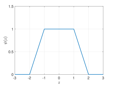
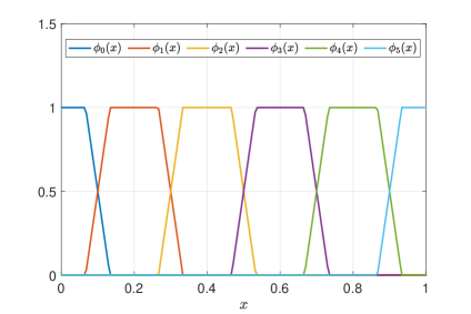
Figure 8: Left: the function $\psi$. Right: the partition of unity (a collection of $n+1=6$ functions) for the case $d=1$ and $n=5$.

The partition of unity $U$ has the following properties:

1. $0\leq\phi_{{\bf m}}({\bf x})\leq 1,\ \ \forall\phi_{{\bf m}}\in U,\ \ \forall{\bf x}\in{\mathbb{R}}^{d}$.

2. $\sum_{\phi_{{\bf m}}\in U}\phi_{{\bf m}}({\bf x})=1,\ \ \forall{\bf x}\in X$.

3. $\text{supp}(\phi_{{\bf m}})\subset\{{\bf x}:\,|x_{\ell}-\frac{m_{\ell}}{n}|<\frac{1}{n},\,\ell=1,\dotsc,d\}=:B_{{\bf m}}^{\infty},\ \ \forall\phi_{{\bf m}}\in U$.

4. $||\phi_{{\bf m}}||_{W^{1,\infty}({\mathbb{R}}^{d})}\leq 4\,n$.

The first three properties follow easily from the definition of $U$. To show the fourth property, we note that $||\phi_{{\bf m}}||_{W^{1,\infty}({\mathbb{R}}^{d})}=||\phi_{{\bf m}}||_{L^{\infty}({\mathbb{R}}^{d})}+||D\phi_{{\bf m}}||_{L^{\infty}({\mathbb{R}}^{d})}$. The first term is bounded by one (thanks to property no. 1). It is also straightforward to show that $\partial\phi_{{\bf m}}/\partial x_{\ell}\leq 3\,n$, by directly computing the derivative of $\phi_{{\bf m}}$ with respect to each coordinate $x_{\ell}$. Hence, the second term is bounded by $3\,n$. We therefore obtain $||\phi_{{\bf m}}||_{W^{1,\infty}({\mathbb{R}}^{d})}\leq 1+3\,n\leq 4\,n$.

Remark 10.

(On the boundary points) For the points on the boundary of $X$ and to construct averaged Taylor polynomials near the boundary of $X$ one possibility is to use an extension operator and extend the function $f$ slightly outside the domain $X$. This would introduce tedious technicalities in the exposition of formulas and proofs, and hence we avoid it here. Instead, we assume that $\phi_{{\bf m}}$ for ${\bf m}$ on the boundary vanishes outside $X$; see e.g. $\phi_{0}$ and $\phi_{5}$ in Figure 8. Similarly, we assume that the definition of $B_{{\bf m}}^{\infty}$ is modified by $B_{{\bf m}}^{\infty}\cap X$ for any ${\bf m}$ on the boundary. With such modifications, we will have $\cup_{{\bf m}}B_{{\bf m}}^{\infty}=X$. The same modification is assumed to be applied to all balls near the boundary over which we compute averaged Taylor polynomials.

14.6 Construction of a global polynomial approximant

Now, we will use averaged Taylor polynomials to build a local approximation (and obtain local estimates) and then combine them using the partition of unity to build a global approximation (and obtain a global estimate).

Local approximations. For each multi-index ${\bf m}\in\{0,1,\dotsc,n\}^{d}$, corresponding to a grid point, consider the ball

$$B_{{\bf m}}:=B(\frac{{\bf m}}{n},r=\frac{3}{4n})\subset B_{{\bf m}}^{\infty},$$

where $B_{{\bf m}}^{\infty}$ is defined in property no. 3 in Section 14.5 and contains the support of $\phi_{{\bf m}}$. We note that $B_{{\bf m}}^{\infty}$ is bounded and convex (and in particular star-shaped with respect to the ball $B_{{\bf m}}$). Hence, we can use the Bramble-Hilbert Lemma with $h=\text{diam}(B_{{\bf m}}^{\infty})=2\,\sqrt{d}/n$. Specifically, we let $p_{{\bf m}}$ be the Taylor polynomial of order $k$ of $f$ averaged over $B_{{\bf m}}$ that (thanks to the polynomial property of averaged Taylor polynomials in Section 14.4) can be written as

$$p_{{\bf m}}({\bf x})=\sum_{|\boldsymbol{\alpha}|\leq k-1}c_{{\bf m},\boldsymbol{\alpha}}\,{\bf x}^{\boldsymbol{\alpha}},\qquad{\bf x}\in B_{{\bf m}}^{\infty},$$

where by (19) and noting $r=\frac{3}{4\,n}$,

$$|c_{{\bf m},\boldsymbol{\alpha}}|\leq c(k,d)\,n^{d/p}\,||f||_{W^{k-1,p}(B_{{\bf m}}^{\infty})}.$$

Note that this is a local approximation of $f$, as $p_{{\bf m}}({\bf x})$ is the approximating polynomial defined on $B_{{\bf m}}^{\infty}$, not on the whole domain $X$. By the Bramble-Hilbert Lemma with $h=\text{diam}(B_{{\bf m}}^{\infty})=2\,\sqrt{d}/n$, we get the local estimate (with $s=0$),

$$||f-p_{{\bf m}}||_{L^{p}(B_{{\bf m}}^{\infty})}\leq c(k,d)\,(\frac{1}{n})^{k}\,|f|_{W^{k,p}(B_{{\bf m}}^{\infty})}\leq c(k,d)\,(\frac{1}{n})^{k}\,||f||_{W^{k,p}(B_{{\bf m}}^{\infty})}.$$

A global approximation. We next combine the partition of unity with all local polynomials to build a global polynomial approximation of $f$ on $X$. Specifically, we define the global approximating polynomial

$$f_{n}({\bf x}):=\sum_{{\bf m}}\phi_{{\bf m}}({\bf x})\,p_{{\bf m}}({\bf x}),\qquad{\bf x}\in X,$$

where the sum is taken over all $(n+1)^{d}$ multi-indices ${\bf m}\in\{0,1,\dotsc,n\}^{d}$ and $\{\phi_{{\bf m}}\}$ forms the partition of unity defined in Section 14.5. We can now write

$$||f-f_{n}||_{L^{p}(X)}^{p}=||\sum_{{\bf m}}\phi_{{\bf m}}\,(f-p_{{\bf m}})||_{L^{p}(X)}^{p}\leq\sum_{\tilde{\bf m}}||\sum_{{\bf m}}\phi_{{\bf m}}\,(f-p_{{\bf m}})||_{L^{p}(B_{\tilde{\bf m}}^{\infty})}^{p},$$ (20)

where the last inequality follows from the integral-definition of $L^{p}$-norm and that $X=\cup_{\tilde{\bf m}}B_{\tilde{\bf m}}^{\infty}$.

For each multi-index $\tilde{\bf m}$ we have

$$||\sum_{{\bf m}}\phi_{{\bf m}}\,(f-p_{{\bf m}})||_{L^{p}(B_{\tilde{\bf m}}^{\infty})} \leq\sum_{{\bf m}:\,||{\bf m}-\tilde{{\bf m}}||_{\infty}\leq 1}||\phi_{{\bf m}}\,(f-p_{{\bf m}})||_{L^{p}(B_{\tilde{\bf m}}^{\infty})}$$

$$\leq\sum_{{\bf m}:\,||{\bf m}-\tilde{{\bf m}}||_{\infty}\leq 1}||\phi_{{\bf m}}\,(f-p_{{\bf m}})||_{L^{p}(B_{{\bf m}}^{\infty})},$$

where the first inequality is a result of the triangle inequality and noting that $\text{supp}(\phi_{{\bf m}})\subset B_{{\bf m}}^{\infty}$, implying that we only need to consider multi-indices ${\bf m}$ that are adjacent to $\tilde{{\bf m}}$, because only $\phi_{{\bf m}}$ corresponding to such multi-indices take values on $B_{\tilde{\bf m}}^{\infty}$ and hence contribute to the norm over $B_{\tilde{\bf m}}^{\infty}$. The second inequality is again a consequence of the support of $\phi_{{\bf m}}$, that is,

$$\text{supp}(g)\subset B_{{\bf m}}^{\infty}\quad\Rightarrow\quad||g||_{L^{p}(B_{\tilde{\bf m}}^{\infty})}=||g||_{L^{p}(B_{\tilde{\bf m}}^{\infty}\cap B_{{\bf m}}^{\infty})}\leq||g||_{L^{p}(B_{{\bf m}}^{\infty})}.$$

Each term in the sum in the last inequality above can further be bounded by,

$$||\phi_{{\bf m}}\,(f-p_{{\bf m}})||_{L^{p}(B_{{\bf m}}^{\infty})}\leq||\phi_{{\bf m}}||_{L^{\infty}(B_{{\bf m}}^{\infty})}\,||(f-p_{{\bf m}})||_{L^{p}(B_{{\bf m}}^{\infty})}\leq c(k,d)\,(\frac{1}{n})^{k}\,||f||_{W^{k,p}(B_{{\bf m}}^{\infty})},$$

where we used the local estimates obtained above and the fact that $\phi_{{\bf m}}\leq 1$ everywhere. Combining the last two inequalities we get for each multi-index $\tilde{\bf m}$,

$$||\sum_{{\bf m}}\phi_{{\bf m}}\,(f-p_{{\bf m}})||_{L^{p}(B_{\tilde{\bf m}}^{\infty})}\leq c(k,d)\,(\frac{1}{n})^{k}\,\sum_{{\bf m}:\,||{\bf m}-\tilde{{\bf m}}||_{\infty}\leq 1}||f||_{W^{k,p}(B_{{\bf m}}^{\infty})}.$$ (21)

Now, by (20) and (21), we get

$$||f-f_{n}||_{L^{p}(X)}^{p}\leq c^{p}(k,d)\,(\frac{1}{n})^{kp}\,\sum_{\tilde{\bf m}}\bigl{(}\sum_{{\bf m}:\,||{\bf m}-\tilde{{\bf m}}||_{\infty}\leq 1}||f||_{W^{k,p}(B_{{\bf m}}^{\infty})}\bigr{)}^{p}.$$ (22)

Now, let us recall Hölder’s inequality

$$\sum_{{\bf m}}|g_{{\bf m}}\,h_{{\bf m}}|\leq\bigl{(}\sum_{{\bf m}}|g_{{\bf m}}|^{p}\bigr{)}^{1/p}\,\bigl{(}\sum_{{\bf m}}|h_{{\bf m}}|^{q}\bigr{)}^{1/q},\qquad g_{{\bf m}},\,h_{{\bf m}}\in{\mathbb{R}},\qquad p\in(1,\infty),\qquad\frac{1}{p}+\frac{1}{q}=1.$$

Setting $g_{{\bf m}}:=||f||_{W^{k,p}(B_{{\bf m}}^{\infty})}$ and $h_{{\bf m}}:=1$, and raising both sides of Hölder’s inequality to power $p$, we obtain

$$\bigl{(}\sum_{{\bf m}:\,||{\bf m}-\tilde{{\bf m}}||_{\infty}\leq 1}||f||_{W^{k,p}(B_{{\bf m}}^{\infty})}\bigr{)}^{p}\leq\sum_{{\bf m}:\,||{\bf m}-\tilde{{\bf m}}||_{\infty}\leq 1}||f||_{W^{k,p}(B_{{\bf m}}^{\infty})}^{p}\,(3^{d})^{p/q},$$ (23)

where $3^{d}=\sum_{{\bf m}:\,||{\bf m}-\tilde{{\bf m}}||_{\infty}\leq 1}1$ is the total number of indices ${\bf m}$ that are either adjacent or identical to $\tilde{\bf m}$. By the definition of $B_{{\bf m}}$, it is also not difficult to see that (show this as an exercise),

$$\sum_{\tilde{\bf m}}\,\sum_{{\bf m}:\,||{\bf m}-\tilde{{\bf m}}||_{\infty}\leq 1}||f||_{W^{k,p}(B_{{\bf m}}^{\infty})}^{p}\leq 3^{d}\,\sum_{\tilde{\bf m}}||f||_{W^{k,p}(B_{\tilde{\bf m}}^{\infty})}^{p}.$$ (24)

Moreover, by the definition of $B_{{\bf m}}$ and the integral-definition of $W^{k,p}$-norm, one gets (show this as an exercise),

$$\sum_{\tilde{\bf m}}||f||_{W^{k,p}(B_{\tilde{\bf m}}^{\infty})}^{p}\leq 2^{d}\,||f||_{W^{k,p}(\cup_{\tilde{\bf m}}B_{\tilde{\bf m}}^{\infty})}^{p}=2^{d}\,||f||_{W^{k,p}(X)}^{p}.$$ (25)

Combining (22)-(25), we finally obtain the global estimate

$$||f-f_{n}||_{L^{p}(X)}\leq c(k,d,p)\,(\frac{1}{n})^{k}\,||f||_{W^{k,p}(X)}.$$

We summarize the results of Sections 14.4-14.6 in the following proposition.

Proposition 1.

Let $U=\{\phi_{{\bf m}}:\,{\bf m}\in\{0,1,\dotsc,n\}^{d}\}$, with $\text{supp}(\phi_{{\bf m}})\subset B_{{\bf m}}^{\infty}$ and $\cup_{{\bf m}}B_{{\bf m}}^{\infty}=X$, be the partition of unity over $X=[0,1]^{d}$ built in Section 14.5. Then, for every $f\in W^{k,p}(X)$, with $k\geq 1$ and $p\in[1,\infty]$, there exists a polynomial

$$f_{n}({\bf x}):=\sum_{{\bf m}}\phi_{{\bf m}}({\bf x})\,p_{{\bf m}}({\bf x}),\qquad{\bf x}\in X,$$

with

$$p_{{\bf m}}({\bf x})=\sum_{|\boldsymbol{\alpha}|\leq k-1}c_{{\bf m},\boldsymbol{\alpha}}\,{\bf x}^{\boldsymbol{\alpha}},\qquad{\bf x}\in B_{{\bf m}}^{\infty},\qquad|c_{{\bf m},\boldsymbol{\alpha}}|\leq c(k,d)\,n^{d/p}\,||f||_{W^{k-1,p}(B_{{\bf m}}^{\infty})},$$

that satisfies

$$||f-f_{n}||_{L^{p}(X)}\leq c(k,d,p)\,(\frac{1}{n})^{k}\,||f||_{W^{k,p}(X)}.$$ (26)

14.7 Expressive power of ReLU networks: an intuitive example

We consider the quadratic function on the interval $[0,1]$, displayed in Figure 9,

$$g(x)=x^{2},\qquad x\in[0,1].$$

Our goal is to construct a ReLU network approximant, say $\tilde{g}$, of $g$ with the error

$$||g-\tilde{g}||_{L^{\infty}([0,1])}\leq\varepsilon,$$ (27)

with minimal complexity, i.e. with the number of layers, neurons, and parameters as small as possible. Indeed, we will show that this can be achieved with complexity $L,N,P={\mathcal{O}}(\varepsilon^{-1})$. Our construction will use the “sawtooth” function that (first) appeared in [29].

Figure 9: The quadratic function $g(x)=x^{2}$ on the interval $[0,1]$ to be approximated by a ReLU network.

Sawtooth function made by the composition of hat functions. Consider the hat function (also known as tent or triangle function), displayed in Figure 10,

$$h(x)=\left\{\begin{array}[]{l l}2\,x,&\qquad 0\leq x<1/2,\\ 2(1-x),&\qquad 1/2\leq x\leq 1,\\ 0,&\qquad\text{elsewhere}.\end{array}\right.$$

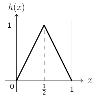
Figure 10: The hat function $h(x)$ on the interval $[0,1]$.

Now let

$$h_{0}(x)=x,\qquad h_{1}(x)=h(x),$$

and denote by $h_{s}(x)$, with $s\geq 2$, the $s$-fold composition of $h$ with itself

$$h_{s}(x)=\underbrace{{h\circ h\circ\dotsc\circ h}}_{s\,\,\text{times}}(x),\qquad s\geq 2.$$

Telgarsky [29] has shown that $h_{s}$ is a sawtooth function with $2^{s-1}$ evenly distributed teeth (or tents), where each application of $h$ doubles the number of teeth; see Figure 11.

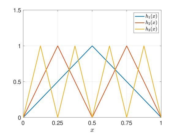
Figure 11: The sawtooth function $h_{s}(x)$ on the interval $[0,1]$ with $s=1,2,3$.

We make two observations and will discuss each in turn:

• $g(x)=x^{2}$ can be approximated by linear combinations of $h_{0},h_{1},h_{2},\dotsc$.

• $h_{0},h_{1},h_{2},\dotsc$ and hence their linear combinations can be expressed by a ReLU network.

Observation 1. We start with approximating $g(x)=x^{2}$ by a piecewise-linear interpolation $g_{m}$ of $g$ on a uniform grid of $2^{m}+1$ evenly distributed grid points $\{\frac{i}{2^{m}}\}_{i=0}^{2^{m}}$; see Figure 12. Note that by definition of interpolation, we have

$$g_{m}(x)=x^{2},\qquad x=\frac{i}{2^{m}},\qquad i=0,1,\dotsc,2^{m}.$$

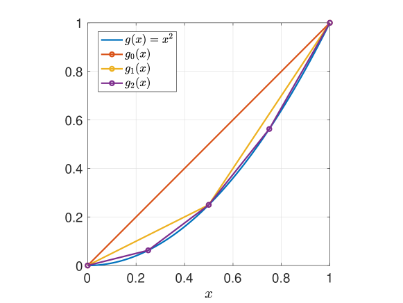
Figure 12: Piecewise-linear approximation $g_{m}(x)$ of $g(x)=x^{2}$ at $2^{m}+1$ evenly distributed grid points on the interval $[0,1]$, with $m=0,1,2$.

It is not difficult to see that refining the interpolation from $g_{m-1}$ to $g_{m}$ amounts to adjusting it by a function proportional to a sawtooth function,

$$g_{m-1}(x)-g_{m}(x)=\frac{h_{m}(x)}{2^{2\,m}}.$$

We hence obtain

$$g_{m}(x)=x-\sum_{s=1}^{m}\frac{h_{s}(x)}{2^{2\,s}}.$$ (28)

That is, the function $g(x)=x^{2}$ can be approximated by linear combinations of $h_{0},h_{1},h_{2},\dotsc$.

It is to be noted that the construction of $g_{m}$ only involves ${\mathcal{O}}(m)$ linear operations and compositions of $h$. This shows the “super power” of composition! For instance, to build $h_{m}$ (and hence $g_{m}$) without composition, we would need ${\mathcal{O}}(2^{m})$ operations. However, using composition, we would only need ${\mathcal{O}}(m)$ operations, a huge reduction from an exponential complexity down to a linear complexity. As we will see later, this is a major reason why deep learning (which involves multiple applications of composition) has been so successful in solving science and engineering problems.

We can also derive a clear formula for the approximation error $||g(x)-g_{m}(x)||_{L^{\infty}([0,1])}$. For this purpose, we will carry out a simple numerical experiment, and show how such numerical experiments could help derive theoretical results. To this end, we will compute the error $|g(x)-g_{m}(x)|$ versus $x\in[0,1]$ for the first three approximations $g_{m}$ with $m=0,1,2$. The result is depicted in Figure 13. Obviously, the initial maximum error is

$$\max_{x\in[0,1]}|g(x)-g_{0}(x)|=\max_{x\in[0,1]}|x^{2}-x|=1/4.$$

This can be easily shown by equating the derivative of $x^{2}-x$ to zero (i.e. $2x-1=0$), which tells us that the maximum is at $x=1/2$ and is equal to $|(1/2)^{2}-(1/2)|=1/4$. Figure 13 also tells us that with increasing $m$ by one, the maximum error gets multiplied by $1/4$. Overall, the figure suggests that the maximum error is $2^{-2(m+1)}$, that is,

$$||g(x)-g_{m}(x)||_{L^{\infty}([0,1])}=2^{-2(m+1)},\qquad m=0,1,2,\dotsc.$$ (29)

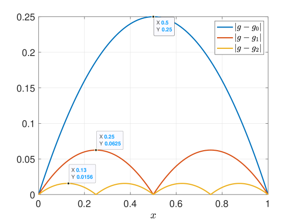
Figure 13: The error $|g(x)-g_{m}(x)|$ in the approximation of $g(x)=x^{2}$ by a piecewise linear interpolant $g_{m}$ at $2^{m}+1$ evenly distributed grid points on the interval $[0,1]$, with $m=0,1,2$. This suggests that with increasing $m$, the maximum error decays as $2^{-2(m+1)}$.

This is indeed an example of the power of numerical experiments in deriving theoretical results. Interestingly, the figure also tells us how to theoretically prove (29). For every $m=0,1,2,\dotsc$, the error $|g(x)-g_{m}(x)|$ is identical on each subinterval between two consecutive points of interpolation. In particular, we will have

$$\max_{x\in[0,1]}|g(x)-g_{m}(x)|=\max_{x\in[0,1/2^{m}]}|g(x)-g_{m}(x)|.$$

It is now straightforward to show (29) using the right hand side of the above formula.

Observation 2. We start the second observation with noting that the hat function $h=h(x)$ can be realized (or expressed) by a ReLU network. To derive such a network, we first note that $h$ can be written as a linear combination of three ReLU functions (see Figure 14):

$$h(x)=2\,\sigma(x)-4\,\sigma(x-1/2)+2\,\sigma(x-1).$$

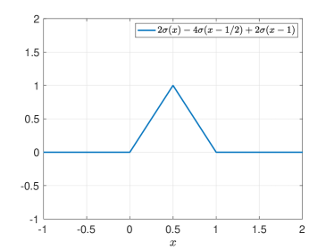
Figure 14: The three ReLU functions (left) that combine to form the har function (right).

One can then easily see that $h(x)$ is given by a ReLU network with $L=2$ layers,

$$\Phi_{h}(x):=A_{2}\circ\sigma\circ A_{1}(x),$$

where

$$A_{1}(x)=\left(\begin{array}[]{c}1\\ 1\\ 1\end{array}\right)\,x+\left(\begin{array}[]{c}0\\ -1/2\\ -1\end{array}\right),\quad A_{2}({\bf z})=(2\ \ -4\ \ 2)\,\left(\begin{array}[]{c}z_{1}\\ z_{2}\\ z_{3}\end{array}\right).$$

Figure 15 shows a graph representation of $\Phi_{h}(x)=h(x)$, with $L=2$ layers, $N=5$ neurons, and $P=10$ parameters (i.e. weights and biases).

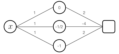
Figure 15: The two-layer ReLU network that realizes $h(x)=2\,\sigma(x)-4\,\sigma(x-1/2)+2\,\sigma(x-1)$.

It will now be straightforward to construct a ReLU network with $L=s+1$ layers that realizes $h_{s}(x)$, for any $s\geq 2$. One such network is given by

$$\Phi_{h_{s}}(x):=A_{s+1}\circ\sigma\circ A_{s}\circ\sigma\circ\dotsc\circ A_{2}\circ\sigma\circ A_{1}(x),$$

where

$$A_{1}(x)=\left(\begin{array}[]{c}1\\ 1\\ 1\end{array}\right)\,x+\left(\begin{array}[]{c}0\\ -1/2\\ -1\end{array}\right),\quad A_{s+1}({\bf z})=(2\ \ -4\ \ 2)\,\left(\begin{array}[]{c}z_{1}\\ z_{2}\\ z_{3}\end{array}\right),$$

and

$$A_{\ell}(x)=\left(\begin{array}[]{c c c}2&-4&2\\ 2&-4&2\\ 2&-4&2\end{array}\right)\,\left(\begin{array}[]{c}z_{1}\\ z_{2}\\ z_{3}\end{array}\right)+\left(\begin{array}[]{c}0\\ -1/2\\ -1\end{array}\right),\qquad\ell=2,\dotsc,s.$$

The complexity of such network is

$$L(\Phi_{h_{s}})=s+1,\qquad N(\Phi_{h_{s}})=3\,s+2,\qquad P(\Phi_{h_{s}})=12\,s-2.$$

Figure 16 shows the graph representation of $\Phi_{h_{2}}(x)=h_{2}(x)$, with $L=3$ layers, $N=8$ neurons, and $P=22$ parameters.

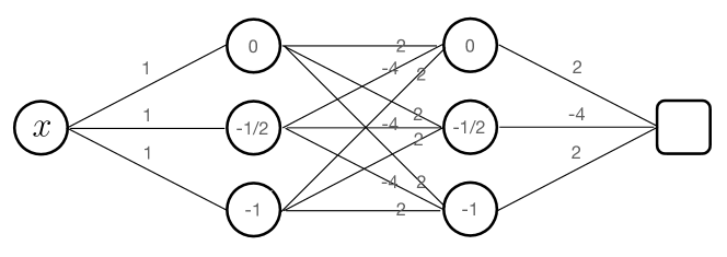
Figure 16: The three-layer ReLU network that realizes $h_{2}(x)$.

Finally, we can construct a ReLU network with $L=m+1$ layers that realizes $g_{m}(x)$, for any $m\geq 1$. One such network is given by

$$\Phi_{g_{m}}(x):=A_{m+1}\circ\sigma\circ A_{m}\circ\sigma\circ\dotsc\circ A_{2}\circ\sigma\circ A_{1}(x),$$

where

$$A_{1}(x)=\left(\begin{array}[]{c}1\\ 1\\ 1\\ 1\end{array}\right)\,x+\left(\begin{array}[]{c}0\\ -1/2\\ -1\\ 0\end{array}\right),\quad A_{m+1}({\bf z})=(-1/2\ \ 1\ \ -1/2\ \ 1)\,\left(\begin{array}[]{c}z_{1}\\ z_{2}\\ z_{3}\\ z_{4}\end{array}\right),$$

and

$$A_{\ell}(x)=\left(\begin{array}[]{c c c c}1/2&-1&1/2&0\\ 1/2&-1&1/2&0\\ 1/2&-1&1/2&0\\ -1/2&1&-1/2&1\end{array}\right)\,\left(\begin{array}[]{c}z_{1}\\ z_{2}\\ z_{3}\\ z_{4}\end{array}\right)+\left(\begin{array}[]{c}0\\ -2^{-2\,\ell+1}\\ -2^{-2\,\ell+2}\\ 0\end{array}\right),\qquad\ell=2,\dotsc,m.$$

The complexity of such network is

$$L(\Phi_{g_{m}})=m+1,\qquad N(\Phi_{g_{m}})=4\,m+2,\qquad P(\Phi_{g_{m}})=20\,m-7.$$

Figure 17 and Figure 18 show the graph representations of $\Phi_{g_{1}}(x)=x-\frac{1}{4}\,h_{1}(x)$ and $\Phi_{g_{2}}(x)=x-\frac{1}{4}\,h_{1}(x)-\frac{1}{16}\,h_{2}(x)$, respectively.

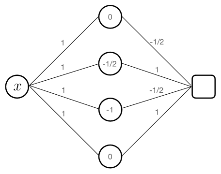
Figure 17: The two-layer ReLU network that realizes $g_{1}(x)=x-\frac{1}{4}\,h_{1}(x)$.

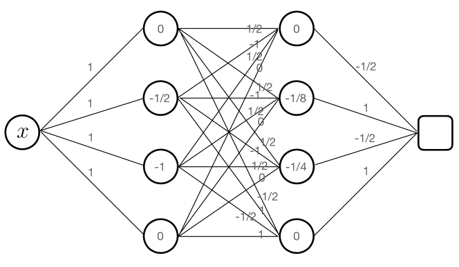
Figure 18: The three-layer ReLU network that realizes $g_{2}(x)=x-\frac{1}{4}\,h_{1}(x)-\frac{1}{16}\,h_{2}(x)$.

We can now state the final result on the approximation of the quadratic function by ReLU networks.

Lemma 2.

The function $g(x)=x^{2}$ on $[0,1]$ can be approximated within any small error $\varepsilon\in(0,1/2)$ in the sense (27) by a ReLU network with complexity $L,M,P={\mathcal{O}}(\log_{2}\varepsilon^{-1})$.

Proof.

The proof follows directly by choosing $m=\lceil\frac{1}{2}\log_{2}\varepsilon^{-1}\rceil$. ∎

Remark 11.

We have discussed how the power of composition in neural networks makes them efficient approximants in the sense that their complexity increases logarithmically with the reciprocal of the approximation error. This is a very desirable approximation property of neural networks. Note that the input dimension is one here, and hence this result does not address the effect of composition on dimension.

14.8 Connected and standard ReLU networks

We closely follow the setup used in [22, 15] and define two classes of feedforward ReLU networks:

• connected networks, where connection is allowed between all layers;

• standard networks, where connection is allowed only between neighboring layers.

The latter, that we have been considering so far, is a particular case of the former. We will also present an important result that states if a function can be realized by a connected network, it can also be realized by a standard network with comparable complexity. In this sense, any accuracy-complexity result obtained for connected networks will also hold for standard networks with minor modifications.

Connected networks. A connected network with $N_{0}=d$ inputs and $L$ layeres, each with $N_{\ell}$ neurons, $\ell=1,\dotsc,L$, is given by a sequence of matrix-vector tuples (or weight-bias tuples)

$$\Phi:=\{(W_{1},b_{1}),\dotsc,(W_{L},b_{L})\},\qquad W_{\ell}\in{\mathbb{R}}^{N_{\ell}\times\sum_{i=0}^{\ell-1}N_{i}},\qquad b_{\ell}\in{\mathbb{R}}^{N_{\ell}}.$$

The weight matrices $W_{\ell}$ may be written in block matrix form

$$W_{\ell}=\bigl{(}W_{\ell,0}\ |\ W_{\ell,1}\ |\ \dotsc\ |\ W_{\ell,\ell-1}\bigr{)}\ \in{\mathbb{R}}^{N_{\ell}\times\sum_{i=0}^{\ell-1}N_{i}},\qquad W_{\ell,i}\in{\mathbb{R}}^{N_{\ell}\times N_{i}}.$$

With a slight abuse of notation, we also use $\Phi$ to denote the function that the network realizes, and write

$$\Phi({\bf x})={\bf x}_{L},\qquad\Phi:{\mathbb{R}}^{d}\rightarrow{\mathbb{R}}^{N_{L}},$$

where ${\bf x}_{L}$ results from the following scheme:

$${\bf x}_{0} ={\bf x},$$

$${\bf x}_{\ell} =\sigma(W_{\ell,0}{\bf x}_{0}+\dotsc+W_{\ell,\ell-1}{\bf x}_{\ell-1}+b_{\ell}),\qquad\ell=1,\dotsc,L-1,$$

$${\bf x}_{L} =W_{L,0}{\bf x}_{0}+\dotsc+W_{L,L-1}{\bf x}_{L-1}+b_{L}.$$

The distinction between $\Phi$ being a function or a set of matrix-vector tuples should be easily made from the context.

As before, we consider ReLU activation function $\sigma:{\mathbb{R}}\rightarrow{\mathbb{R}}$ that acts componentwise on all hidden layers. We do not apply any activation function on the output layer. The complexity of a connected network $\Phi$, represented by the number of layers $L(\Phi)$, number of neurons $N(\Phi)$, and number of non-zero parameters $P(\Phi)$, is given by

$$L(\Phi)=L,\qquad N(\Phi)=\sum_{\ell=0}^{L}N_{\ell},\qquad P(\Phi)=\sum_{\ell=1}^{L}(||W_{\ell}||_{0}+||b_{\ell}||_{0}),\qquad||A||_{0}:=\text{nnz}(A).$$

Standard networks. A standard network with $N_{0}=d$ inputs and $L$ layers, each with $N_{\ell}$ neurons, $\ell=1,\dotsc,L$, is given by a sequence of matrix-vector tuples (or weight-bias tuples)

$$\Phi:=\{(W_{1},b_{1}),\dotsc,(W_{L},b_{L})\},\qquad W_{\ell}\in{\mathbb{R}}^{N_{\ell}\times N_{\ell-1}},\qquad b_{\ell}\in{\mathbb{R}}^{N_{\ell}}.$$

We also denote by $\Phi$ the function that the network realizes, and write

$$\Phi({\bf x})={\bf x}_{L},\qquad\Phi:{\mathbb{R}}^{d}\rightarrow{\mathbb{R}}^{N_{L}},$$

where ${\bf x}_{L}$ results from the following scheme:

$${\bf x}_{0} ={\bf x},$$

$${\bf x}_{\ell} =\sigma(W_{\ell}\,{\bf x}_{\ell-1}+b_{\ell}),\qquad\ell=1,\dotsc,L-1,$$

$${\bf x}_{L} =W_{L}\,{\bf x}_{L-1}+b_{L}.$$

It is to be noted that a standard network is a particular type of connected network whose weight matrices are in the block form

$$W_{\ell}=\bigl{(}\ {\bf 0}\ |\ \dotsc\ |\ {\bf 0}\ |\ W_{\ell,\ell-1}\bigr{)}\ \in{\mathbb{R}}^{N_{\ell}\times\sum_{i=0}^{\ell-1}N_{i}},\qquad W_{\ell,\ell-1}\in{\mathbb{R}}^{N_{\ell}\times N_{\ell-1}}.$$

Identity ReLU network. Let $I_{d}\in{\mathbb{R}}^{d\times d}$ be the identity matrix, i.e. $I_{d}{\bf x}={\bf x}$. Consider the two-layer standard ReLU network

$$\Phi_{I}:=\{(W_{1},b_{1}),(W_{2},b_{2})\},$$

with

$$W_{1}=\left(\begin{array}[]{c}I_{d}\\ -I_{d}\end{array}\right)\in{\mathbb{R}}^{2d\times d},\qquad b_{1}={\bf 0}\in{\mathbb{R}}^{2d},\qquad W_{2}=(I_{d}\ |\ -I_{d})\in{\mathbb{R}}^{d\times 2d},\qquad b_{2}={\bf 0}\in{\mathbb{R}}^{d}.$$

Then, using the identity relation $\sigma(x)-\sigma(-x)=x$, it can easily be shown that

$$\Phi_{I}({\bf x})=I_{d}\,{\bf x}={\bf x}.$$

We hence call $\Phi_{I}$ the identity ReLU network.

Composition of networks. Consider two (connected) networks

$$\Phi_{1}=\{(W_{1}^{1},b_{1}^{1}),\dotsc,(W_{L_{1}}^{1},b_{L_{1}}^{1})\},\qquad\Phi_{2}=\{(W_{1}^{2},b_{1}^{2}),\dotsc,(W_{L_{2}}^{2},b_{L_{2}}^{2})\},$$

where the input dimension of $\Phi_{1}$ is equal to the output dimension of $\Phi_{2}$, and $\Phi_{2}$ takes ${\bf x}\in{\mathbb{R}}^{d}$ as input. Then, an efficient way of constructing a (connected) network that gives the composition $\Phi_{1}\circ\Phi_{2}$ is by utilizing the identity network as $\Phi_{1}\circ\Phi_{I}\circ\Phi_{2}$. Such a composition network is given by

$$\Phi_{1}\odot\Phi_{2}:=\Bigl{\{}(W_{1}^{2},b_{1}^{2}),\dotsc,(W_{L_{2}-1}^{2},b_{L_{2}-1}^{2}),\bigl{(}\left(\begin{array}[]{c}W_{L_{2}}^{2}\vspace{0.3cm}\\ -W_{L_{2}}^{2}\end{array}\right),\left(\begin{array}[]{c}b_{L_{2}}^{2}\vspace{0.3cm}\\ -b_{L_{2}}^{2}\end{array}\right)\bigr{)},(\hat{W}_{1}^{1},b_{1}^{1}),\dotsc,(\hat{W}_{L_{1}}^{1},b_{L_{1}}^{1})\Bigr{\}},$$

where

$$\hat{W}_{\ell}^{1}=\bigl{(}{\bf 0}\ |\ W_{\ell,0}^{1}\ |\ -W_{\ell,0}^{1}\ |\ W_{\ell,1}^{1}\ |\ \dotsc\ |\ W_{\ell,\ell-1}^{1}\bigr{)},\qquad\ell=1,\dotsc,L_{1}.$$

We have

$$\Phi_{1}\odot\Phi_{2}({\bf x})=\Phi_{1}\circ\Phi_{2}({\bf x}),\qquad{\bf x}\in{\mathbb{R}}^{d}.$$

Furthermore, we have

$$L(\Phi_{1}\odot\Phi_{2})=L_{1}+L_{2},\quad N(\Phi_{1}\odot\Phi_{2})\leq 2\,N(\Phi_{1})+2\,N(\Phi_{2}),\quad P(\Phi_{1}\odot\Phi_{2})\leq 2\,P(\Phi_{1})+2\,P(\Phi_{2}).$$

Combination (or concatenation) of networks. Consider two (connected) networks

$$\Phi_{1}=\{(W_{1}^{1},b_{1}^{1}),\dotsc,(W_{L_{1}}^{1},b_{L_{1}}^{1})\},\qquad\Phi_{2}=\{(W_{1}^{2},b_{1}^{2}),\dotsc,(W_{L_{2}}^{2},b_{L_{2}}^{2})\},$$

which take the same input ${\bf x}\in{\mathbb{R}}^{d}$. We want to construct a network $P(\Phi_{1},\Phi_{2})$ such taht it takes the same input and gives the outputs of the two networks, that is,

$$\Phi_{1}\mathbin{\|}\Phi_{2}({\bf x})=(\Phi_{1}({\bf x}),\Phi_{2}({\bf x})),\qquad{\bf x}\in{\mathbb{R}}^{d}.$$

Assuming $L_{1}\leq L_{2}$, such a combination network is given by

$$\Phi_{1}\mathbin{\|}\Phi_{2}:=\{(\tilde{W}_{1},\tilde{b}_{1}),\dotsc,(\tilde{W}_{L_{2}},\tilde{b}_{L_{2}})\},$$

where

$$\tilde{W}_{\ell}=\Biggl{(}\ \left(\begin{array}[]{c}W_{\ell,0}^{1}\vspace{0.3cm}\\ W_{\ell,0}^{2}\end{array}\right)\ \Biggl{|}\ \left(\begin{array}[]{c c}W_{\ell,1}^{1}&{\bf 0\vspace{0.3cm}}\\ {\bf 0}&W_{\ell,1}^{2}\end{array}\right)\ \Biggl{|}\ \dotsc\ \Biggl{|}\ \left(\begin{array}[]{c c}W_{\ell,\ell-1}^{1}&{\bf 0\vspace{0.3cm}}\\ {\bf 0}&W_{\ell,\ell-1}^{2}\end{array}\right)\ \Biggr{)},\quad\tilde{b}_{\ell}=\left(\begin{array}[]{c}b_{\ell}^{1}\vspace{0.3cm}\\ b_{\ell}^{2}\end{array}\right),\quad 1\leq\ell<L_{1},$$

$$\tilde{W}_{\ell}=\bigl{(}\ W_{\ell,0}^{2}\ |\ ({\bf 0}\ W_{\ell,1}^{2})\ |\ \dotsc\ |\ ({\bf 0}\ W_{\ell,L_{1}-1}^{2})\ |\ W_{\ell,L_{1}}^{2}\ |\ \dotsc\ |\ W_{\ell,\ell-1}^{2}\ \bigr{)},\quad\tilde{b}_{\ell}=b_{\ell}^{2},\quad L_{1}\leq\ell<L_{2},$$

$$\tilde{W}_{L_{2}}=\Biggl{(}\left(\begin{array}[]{c}W_{L_{1},0}^{1}\vspace{0.3cm}\\ W_{L_{2},0}^{2}\end{array}\right)\Biggl{|}\left(\begin{array}[]{c c}W_{L_{1},1}^{1}&{\bf 0\vspace{0.3cm}}\\ {\bf 0}&W_{L_{2},1}^{2}\end{array}\right)\Biggl{|}\dotsc\Biggl{|}\left(\begin{array}[]{c c}W_{L_{1},L_{1}-1}^{1}&{\bf 0\vspace{0.3cm}}\\ {\bf 0}&W_{L_{2},L_{1}-1}^{2}\end{array}\right)\Biggl{|}\left(\begin{array}[]{c}{\bf 0\vspace{0.3cm}}\\ W_{L_{2},L_{1}}^{2}\end{array}\right)\Biggl{|}\dotsc\Biggl{|}\left(\begin{array}[]{c}{\bf 0\vspace{0.3cm}}\\ W_{L_{2},L_{2}-1}^{2}\end{array}\right)\Biggr{)},$$

$$\tilde{b}_{L_{2}}=\left(\begin{array}[]{c}b_{L_{1}}^{1}\vspace{0.3cm}\\ b_{L_{2}}^{2}\end{array}\right).$$

Furthermore, we have

$$L(\Phi_{1}\mathbin{\|}\Phi_{2})=\max\{L_{1},L_{2}\},\quad N(\Phi_{1}\mathbin{\|}\Phi_{2})=N(\Phi_{1})+N(\Phi_{2})-d,\quad P(\Phi_{1}\mathbin{\|}\Phi_{2})=P(\Phi_{1})+P(\Phi_{2}).$$

Connection between connected and standard networks. We will now present a result that states if a function can be realized by a connected network, it can also be realized by a standard network with comparable complexity.

Lemma 3.

For any connected network $\Phi_{c}$ there is a standard network $\Phi_{s}$ with the same input dimension such that

$$\Phi_{s}({\bf x})=\Phi_{c}({\bf x}),\qquad{\bf x}\in{\mathbb{R}}^{d},$$

and

$$L(\Phi_{s})=L(\Phi_{c})=L,\qquad N(\Phi_{s})\leq C\,L\,N(\Phi_{c}),\qquad P(\Phi_{s})\leq C\,(L\,N(\Phi_{c})+P(\Phi_{c})),$$

where $C>0$ is a constant.

Proof.

For the proof refer to the proof of Lemma 2.11 in [15]. ∎

Lemma 3 enables us to switch between connected and standard networks as desired.

14.9 Approximating product of two numbers by ReLU networks

Now consider two real numbers $x\in{\mathbb{R}}$ and $y\in{\mathbb{R}}$, where $\max\{|x|,|y|\}\leq D$, with $D\geq 1$. Note that the case $D<1$ can always be replaced by $D=1$ and hence falls into the case $D\geq 1$ that we consider here. Utilizing the identity formula $xy=\frac{1}{2}((x+y)^{2}-x^{2}-y^{2})$ and the approximation of the quadratic function by ReLU networks discussed in Section 14.7 we show that the product $xy$ can be well approximated by a ReLU network.

Lemma 4.

The function $g(x,y)=xy$ on the domain $[-D,D]^{2}$, where $D\geq 1$, can be approximated by a ReLU network $\Phi_{\varepsilon}^{xy}$ within any small error $\varepsilon\in(0,1/2)$ in the sense

$$||\Phi_{\varepsilon}^{xy}(x,y)-xy||_{L^{\infty}([-D,D]^{2})}\leq\varepsilon,$$

where the network has two input dimensions (one for $x$ and one for $y$) and has the complexity $L,M,P={\mathcal{O}}(\log_{2}\varepsilon^{-1}+\log_{2}D)$. Moreover, if $x=0$ or $y=0$, then $\Phi_{\varepsilon}^{xy}(x,y)=0$.

Proof.

Let $\Phi_{\delta}$ be the network from Lemma 2 that approximates the quadratic function such that

$$||\Phi_{\delta}(z)-z^{2}||_{L^{\infty}([0,1])}\leq\delta,\qquad z\in[0,1],$$

with complexity

$$L(\Phi_{\delta}),N(\Phi_{\delta}),P(\Phi_{\delta})={\mathcal{O}}(\log_{2}\delta^{-1}).$$

Noting that $xy=\frac{1}{2}((x+y)^{2}-x^{2}-y^{2})$, we write

$$xy=4D^{2}\frac{x}{2D}\frac{y}{2D}=2D^{2}((\frac{x+y}{2D})^{2}-(\frac{x}{2D})^{2}-(\frac{y}{2D})^{2}),$$

and set

$$\Phi_{\varepsilon}^{xy}(x,y)=2D^{2}\bigl{(}\Phi_{\delta}(\frac{|x+y|}{2D})-\Phi_{\delta}(\frac{|x|}{2D})-\Phi_{\delta}(\frac{|y|}{2D})\bigr{)}.$$

With this setup, it easily follows that $\Phi_{\varepsilon}^{xy}(x,y)=0$ if $x=0$ or $y=0$. Moreover, we will have

$$||\Phi_{\varepsilon}^{xy}(x,y)-xy||_{L^{\infty}([-D,D]^{2})}\leq 6D^{2}C_{0}||\Phi_{\delta}(z)-z^{2}||_{L^{\infty}([0,1])}\leq\varepsilon,$$

provided we choose $\delta=\varepsilon/(6D^{2}C_{0})$. Here, $C_{0}>0$ is the constant in the inequality

$$||f_{1}\circ f_{2}||_{L^{\infty}(\Omega_{2})}\leq C_{0}\,||f_{1}||_{L^{\infty}(\Omega_{1})}\,||f_{2}||_{L^{\infty}(\Omega_{2})},\qquad f_{1}:\Omega_{1}\subset{\mathbb{R}}\rightarrow{\mathbb{R}},\quad f_{2}:\Omega_{2}\subset{\mathbb{R}}^{2}\rightarrow{\mathbb{R}},$$

where $\Omega_{1}$ and $\Omega_{2}$ are compact, convex sets. In our case, we have $\Omega_{1}=[0,1]$ and $\Omega_{2}=[-D,D]^{2}$. It remains to show that the complexity of $\Phi_{\varepsilon}^{xy}$ is of the same order as the complexity of $\Phi_{\delta}$. We can do this in a constructive way by building the network. By the identity formula $|x|=\sigma(x)+\sigma(-x)$, the network $\Phi_{\varepsilon}^{xy}$ has the complexity (show this as an exercise),

$$L(\Phi_{\varepsilon}^{xy})=L(\Phi_{\delta})+2,\quad N(\Phi_{\varepsilon}^{xy})=3N(\Phi_{\delta})+9,\quad P(\Phi_{\varepsilon}^{xy})=3P(\Phi_{\delta})+23.$$

Then we have

$$L(\Phi_{\varepsilon}^{xy}),N(\Phi_{\varepsilon}^{xy}),P(\Phi_{\varepsilon}^{xy})={\mathcal{O}}(\log_{2}\delta^{-1})={\mathcal{O}}(\log_{2}\varepsilon^{-1}+\log_{2}D),$$

which completes the proof of the lemma. ∎

14.10 ReLU networks and the product of their output components

Utilizing the result obtained in Section 14.9, we now discuss an interesting result on the approximation of the product of the output components of a network by another network with one output.

Lemma 5.

Let $\varepsilon\in(0,1/2)$. Let $\Phi$ be a network with $d$ inputs, $m$ outputs, and complexity $L,N,P\leq M$, and suppose its output components $\Phi_{1},\dotsc,\Phi_{m}$ are all bounded

$$||\Phi_{i}||_{L^{\infty}([0,1]^{d})}\leq 1,\qquad i=1,\dotsc,m.$$

Then, there exists a network $\Psi_{\varepsilon}$ with $d$ inputs, one output, and complexity $L,N,P\leq M\,C(m)\,\log_{2}\varepsilon^{-1}$ such that

$$||\Psi_{\varepsilon}({\bf x})-\prod_{i=1}^{m}\Phi_{i}({\bf x})||_{L^{\infty}([0,1]^{d})}\leq m\,\varepsilon.$$

Moreover, $\Psi_{\varepsilon}({\bf x})=0$ if $\prod_{i=1}^{m}\Phi_{i}({\bf x})=0$, for ${\bf x}\in[0,1]^{d}$.

Proof.

The proof is by induction. For $m=1$, we clearly have $\Psi_{\varepsilon}=\Phi$. Suppose the theorem holds for $m\geq 1$. We show that it also holds for $m+1$. Let

$$\Phi=\{(W_{1},b_{1}),\dotsc,(W_{L},b_{L})\},$$

be a network with $d$ inputs, $m+1\geq 2$ outputs, and complexity $L,N,P\leq M$. In particular, it will be useful to note that we have

$$W_{L}=\left(\begin{array}[]{c}W_{L}^{(1:m)}\vspace{0.3cm}\\ W_{L}^{(m+1)}\end{array}\right)\in{\mathbb{R}}^{(m+1)\times\sum_{\ell=0}^{L-1}N_{\ell}},\qquad W_{L}^{(1:m)}\in{\mathbb{R}}^{m\times\sum_{\ell=0}^{L-1}N_{\ell}},\qquad W_{L}^{(m+1)}\in{\mathbb{R}}^{1\times\sum_{\ell=0}^{L-1}N_{\ell}},$$

and

$$b_{L}=\left(\begin{array}[]{c}b_{L}^{(1:m)}\vspace{0.3cm}\\ b_{L}^{(m+1)}\end{array}\right)\in{\mathbb{R}}^{m+1},\qquad b_{L}^{(1:m)}\in{\mathbb{R}}^{m},\qquad b_{L}^{(m+1)}\in{\mathbb{R}}.$$

Now set

$$\hat{\Phi}=\{(W_{1},b_{1}),\dotsc,(W_{L-1,}b_{L-1}),(W_{L}^{(1:m)},b_{L}^{(1:m)})\},$$

be the network with $d$ inputs and $m$ outputs, formed by removing the last output neuron and its corresponding weights of $\Phi$. Note that the outputs of $\hat{\Phi}$ are precisely the first $m$ outputs of $\Psi$. By induction hypothesis, there exists a network with one output

$$\hat{\Psi}_{\varepsilon}=\{(\hat{W}_{1},\hat{b}_{1}),\dotsc,(\hat{W}_{\hat{L}},\hat{b}_{\hat{L}})\},\qquad\hat{L}\geq L,$$

with the same first $L-1$ layers as in $\hat{\Phi}$ and hence the same first $L-1$ layers as in $\Phi$ such that

$$||\hat{\Psi}_{\varepsilon}-\prod_{i=1}^{m}\Phi_{i}||_{L^{\infty}([0,1]^{d})}=||\hat{\Psi}_{\varepsilon}-\prod_{i=1}^{m}\hat{\Phi}_{i}||_{L^{\infty}([0,1]^{d})}\leq m\,\varepsilon.$$

We modify $\hat{\Psi}_{\varepsilon}$ by adding the removed neuron and its corresponding weights to the last layer of $\hat{\Psi}_{\varepsilon}$, and define a new network with two outputs

$$\tilde{\Psi}_{\varepsilon}=\{(\hat{W}_{1},\hat{b}_{1}),\dotsc,(\hat{W}_{\hat{L}-1},\hat{b}_{\hat{L}-1}),(\tilde{W}_{\hat{L}},\tilde{b}_{\hat{L}})\},\quad\tilde{W}_{\hat{L}}=\left(\begin{array}[]{r c l}&\hat{W}_{\hat{L}}&\vspace{0.3cm}\\ W_{L}^{(m+1)}&&{\bf 0}\end{array}\right),\quad\tilde{b}_{\hat{L}}=\left(\begin{array}[]{c}\hat{b}_{\hat{L}}\vspace{0.3cm}\\ b_{L}^{(m+1)}\end{array}\right).$$

Note that the first output component of $\tilde{\Psi}_{\varepsilon}$ is the same as the only output component of $\hat{\Psi}_{\varepsilon}$. We have

$$||(\tilde{\Psi}_{\varepsilon})_{1}||_{L^{\infty}([0,1]^{d})}=||\hat{\Psi}_{\varepsilon}||_{L^{\infty}([0,1]^{d})}\leq||\hat{\Psi}_{\varepsilon}-\prod_{i=1}^{m}\Phi_{i}||_{L^{\infty}([0,1]^{d})}+||\prod_{i=1}^{m}\Phi_{i}||_{L^{\infty}([0,1]^{d})}\leq m\,\varepsilon+1,$$

and

$$||(\tilde{\Psi}_{\varepsilon})_{2}||_{L^{\infty}([0,1]^{d})}=||\Phi_{m+1}||_{L^{\infty}([0,1]^{d})}\leq 1.$$

We can hence use Lemma 4 with $D=m+1$ and construct the desired network as

$$\Psi_{\varepsilon}:\Phi_{\varepsilon}^{xy}\odot\tilde{\Psi}_{\varepsilon}.$$

It is easy to see that the complexity of network is as desired (verify this). We now work out the approximation error and write

$$||\Psi_{\varepsilon}-\prod_{i=1}^{m+1}\Phi_{i}||_{L^{\infty}([0,1]^{d})} =||\Phi_{\varepsilon}^{xy}\circ\tilde{\Psi}_{\varepsilon}-\Phi_{m+1}\prod_{i=1}^{m}\Phi_{i}||_{L^{\infty}([0,1]^{d})}$$

$$\leq||\Phi_{\varepsilon}^{xy}\circ\tilde{\Psi}_{\varepsilon}-\Phi_{m+1}\,\hat{\Psi}_{\varepsilon}||_{L^{\infty}([0,1]^{d})}+||\Phi_{m+1}\,(\hat{\Psi}_{\varepsilon}-\prod_{i=1}^{m}\Phi_{i})||_{L^{\infty}([0,1]^{d})}.$$

The first term in the right hand side of the above inequality is bounded by $\varepsilon$ thanks to Lemma 4 with $D=m+1$. The second term can also be bounded as

$$||\Phi_{m+1}\,(\hat{\Psi}_{\varepsilon}-\prod_{i=1}^{m}\Phi_{i})||_{L^{\infty}([0,1]^{d})}\leq||\Phi_{m+1}||_{L^{\infty}([0,1]^{d})}\,||\hat{\Psi}_{\varepsilon}-\prod_{i=1}^{m}\Phi_{i}||_{L^{\infty}([0,1]^{d})}\leq m\,\varepsilon,$$

thanks to the induction hypothesis. It hence follows that

$$||\Psi_{\varepsilon}-\prod_{i=1}^{m+1}\Phi_{i}||_{L^{\infty}([0,1]^{d})}\leq(m+1)\,\varepsilon.$$

And this completes the proof. ∎

14.11 ReLU networks and the partition of unity

We now return to the partition of unity and construct a two-layer network $\Phi_{\bf m}$ with $d$ inputs, $d$ outputs, and complexity $N,P={\mathcal{O}}(d)$ such that the product of its output component realizes a function $\phi_{\bf m}\in U$ in the partition of unity; see Section 14.5, that is,

$$\prod_{i=1}^{d}(\Phi_{\bf m})_{i}({\bf x})=\phi_{\bf m}({\bf x}),\qquad{\bf x}\in[0,1]^{d}.$$

Step 1. Construct a two-layer network $\Phi_{\psi}$ that realizes the function $\psi$ over ${\mathbb{R}}$, i.e. $\Phi_{\psi}(z)=\psi(z)$, for $z\in{\mathbb{R}}$; see Figure 19. It is easy to verify that the output of the network is

$$\Phi_{\psi}(z)=\sigma(z+2)-\sigma(z+1)-\sigma(z-1)+\sigma(z-2)=\psi(z),\qquad z\in{\mathbb{R}}.$$

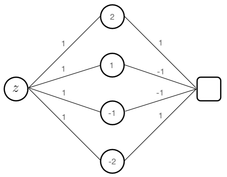
Figure 19: The two-layer ReLU network that realizes $\psi(z)$ for $z\in{\mathbb{R}}$.

The network $\Phi_{\psi}$ has the complexity $L=2$, $N=6$, and $P=12$.

Step 2. By modifying the network in step 1, construct a two-layer network $\Phi_{\psi}^{(i)}$ that realizes $\psi(3\,n\,(x_{i}-\frac{m_{i}}{n}))$; see Figure 20. It is easy to verify that

$$\Phi_{\psi}^{(i)}(x_{i})=\psi(3\,n\,(x_{i}-\frac{m_{i}}{n})),\qquad x_{i}\in[0,1].$$

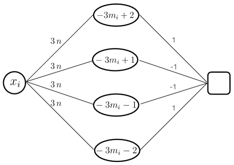
Figure 20: The two-layer ReLU network that realizes $\psi(3\,n\,(x_{i}-\frac{m_{i}}{n}))$ for $x_{i}\in[0,1]$.

The network $\Phi_{\psi}^{(i)}$ has the complexity $L=2$, $N=6$, and $P=12$.

Step 3. Simply stack up the $d$ networks $\Phi_{\psi}^{(1)},\dotsc,\Phi_{\psi}^{(d)}$ constructed in Step 2 in a vertical position (one below another) to build the desired two-layer network $\Phi_{\bf m}$, with complexity $N(\Phi_{\bf m})=6\,d$ and $P(\Phi_{\bf m})=12\,d$.

14.12 Approximating global polynomials by ReLU networks

We are now ready to complete Part 2 of the proof strategy in Section 14.3.

Specifically, we will construct a ReLU network that approximates the global polynomial $f_{n}$ from Proposition 1, constructed in Section 14.6, and obtain an estimation for the error.

Proposition 2.

Let $f_{n}({\bf x})=\sum_{{\bf m}}\sum_{|\boldsymbol{\alpha}|\leq k-1}c_{{\bf m},\boldsymbol{\alpha}}\,\phi_{{\bf m}}({\bf x})\,{\bf x}^{\boldsymbol{\alpha}}$ be the global polynomial from Proposition 1 that approximates $f\in W^{k,p}(X)$, with $k\geq 1$ and $p\in[1,\infty]$, where ${\bf x}\in X=[0,1]^{d}$. Let $\varepsilon\in(0,1/2)$. Then, there exists a ReLU network $\Phi_{\varepsilon}$ with $d$ inputs, one output, and complexity

$$L(\Phi_{\varepsilon})\leq C_{1}(k,d)\,\log_{2}\varepsilon^{-1},\qquad N(\Phi_{\varepsilon}),P(\Phi_{\varepsilon})\leq C_{2}(k,d)\,(n+1)^{d}\,\log_{2}\varepsilon^{-1},$$

such that

$$||f_{n}-\Phi_{\varepsilon}||_{L^{p}(X)}\leq C(k,d,p)\,||f||_{W^{k-1,p}(X)}\,\varepsilon.$$

Proof.

We first approximate the localized terms $\phi_{\bf m}({\bf x})\,{\bf x}^{\boldsymbol{\alpha}}$ for a fixed $({\bf m},\boldsymbol{\alpha})$, where $|\boldsymbol{\alpha}|\leq k-1$, by a ReLU network $\Psi_{\varepsilon,{\bf m},\boldsymbol{\alpha}}$ as follows:

• There is a one-layer ReLU network $\Phi_{\boldsymbol{\alpha}}$ with $d$ input, $|\boldsymbol{\alpha}|$ outputs, and at most $d+k-1$ neurons and at most $k-1$ weights such that

  $${\bf x}^{\boldsymbol{\alpha}}=\prod_{i=1}^{|\boldsymbol{\alpha}|}(\Phi_{\boldsymbol{\alpha}})_{i}({\bf x}),\qquad||(\Phi_{\boldsymbol{\alpha}})_{i}||_{L^{\infty}(X)}\leq 1,\qquad{\bf x}\in X=[0,1]^{d}.$$

• From Section 14.11, we know that there is a two-layer network $\Phi_{\bf m}$ with $d$ inputs, $d$ outputs, $6d$ neurons, and $12d$ parameters such that

  $$\phi_{\bf m}({\bf x})=\prod_{i=1}^{d}(\Phi_{\bf m})_{i}({\bf x}),\qquad||(\Phi_{\bf m})_{i}||_{L^{\infty}(X)}\leq 1,\qquad{\bf x}\in X=[0,1]^{d}.$$

• We concatenate the above two networks and build a network $\Phi_{{\bf m},\boldsymbol{\alpha}}:=\Phi_{\boldsymbol{\alpha}}\mathbin{\|}\Phi_{\bf m}$ that will have two layers, $d$ inputs, $d+|\boldsymbol{\alpha}|$ outputs, at most $6d+k-1$ neurons, and at most $12d+k-1$ parameters, such that

  $$\phi_{\bf m}({\bf x})\,{\bf x}^{\boldsymbol{\alpha}}=\prod_{i=1}^{|\boldsymbol{\alpha}|+d}(\Phi_{{\bf m},\boldsymbol{\alpha}})_{i}({\bf x}),\qquad||(\Phi_{{\bf m},\boldsymbol{\alpha}})_{i}||_{L^{\infty}(X)}\leq 1,\qquad{\bf x}\in X=[0,1]^{d}.$$

• By Lemma 5, there is a ReLU network $\Psi_{\varepsilon,{\bf m},\boldsymbol{\alpha}}$ with $d$ inputs, one output, and complexity

  $$L(\Psi_{\varepsilon,{\bf m},\boldsymbol{\alpha}}),\,N(\Psi_{\varepsilon,{\bf m},\boldsymbol{\alpha}}),\,P(\Psi_{\varepsilon,{\bf m},\boldsymbol{\alpha}})\leq\hat{C}(k,d)\,\log_{2}\varepsilon^{-1},$$

  such that

  $$||\Psi_{\varepsilon,{\bf m},\boldsymbol{\alpha}}-\prod_{i=1}^{|\boldsymbol{\alpha}|+d}(\Phi_{{\bf m},\boldsymbol{\alpha}})_{i}||_{L^{\infty}(X)}\leq C^{\prime}(k,d)\,\varepsilon,$$ (30)

  and $\Psi_{\varepsilon,{\bf m},\boldsymbol{\alpha}}({\bf x})=0$ if $\phi_{\bf m}({\bf x})\,{\bf x}^{\boldsymbol{\alpha}}=0$, for ${\bf x}\in X$.

We next approximate the global polynomial, i.e. the sums of localized polynomials, by a ReLU network $\Phi_{\varepsilon}$ as follows:

• Let $\Lambda:=\{({\bf m},\boldsymbol{\alpha}):\ {\bf m}\in\{0,1,\dotsc,n\}^{d},\ |\boldsymbol{\alpha}|\leq k-1\}$, noting that $|\Lambda|=\tilde{C}(k,d)\,(n+1)^{d}$.

• Let $\Phi_{\text{sum}}$ be the one-layer ReLU network that takes $|\Lambda|$ inputs and gives their weighted sum with the weights $c_{{\bf m},\boldsymbol{\alpha}}$. That is, $\Phi_{\text{sum}}:=\{(W,{\bf 0})\}$, where $W\in{\mathbb{R}}^{1\times|\Lambda|}$ is the matrix with components $c_{{\bf m},\boldsymbol{\alpha}}\in\Lambda$.

• Let $\Phi_{\varepsilon}:=\Phi_{\text{sum}}\odot\bigl{(}{\mathbin{\|}}_{({\bf m},\boldsymbol{\alpha})\in\Lambda}\Psi_{\varepsilon,{\bf m},\boldsymbol{\alpha}}\bigr{)}$, where ${\mathbin{\|}}_{({\bf m},\boldsymbol{\alpha})\in\Lambda}$ denotes network concatenation over all elements of the set $\Lambda$. Clearly, $\Phi_{\varepsilon}$ is a ReLU network with $d$ inputs, one output, number of layers

  $$L(\Phi_{\varepsilon})\leq 1+\hat{C}(k,d)\,\log_{2}\varepsilon^{-1}\leq C_{1}(k,d)\,\log_{2}\varepsilon^{-1},$$

  and number of neurons and parameters

  $$N(\Phi_{\varepsilon}),M(\Phi_{\varepsilon})\leq 2|\Lambda|(1+\hat{c}(k,d)\log_{2}\varepsilon^{-1})\leq C_{2}(k,d)\,(n+1)^{d}\,\log_{2}\varepsilon^{-1},$$

  satisfying

  $$\Phi_{\varepsilon}({\bf x})=\sum_{{\bf m}}\sum_{|\boldsymbol{\alpha}|\leq k-1}c_{{\bf m},\boldsymbol{\alpha}}\,\Psi_{\varepsilon,{\bf m},\boldsymbol{\alpha}}({\bf x}).$$

It remains to derive the approximation error. We write

$$||f_{n}-\Phi_{\varepsilon}||_{L^{p}(X)}^{p} =||\sum_{{\bf m}}\sum_{|\boldsymbol{\alpha}|\leq k-1}c_{{\bf m},\boldsymbol{\alpha}}\,\bigl{(}\phi_{{\bf m}}({\bf x})\,{\bf x}^{\boldsymbol{\alpha}}-\Psi_{\varepsilon,{\bf m},\boldsymbol{\alpha}}({\bf x})\bigr{)}||_{L^{p}(X)}^{p}$$

$$\leq\sum_{\tilde{\bf m}}||\sum_{{\bf m}}\sum_{|\boldsymbol{\alpha}|\leq k-1}c_{{\bf m},\boldsymbol{\alpha}}\,\bigl{(}\phi_{{\bf m}}({\bf x})\,{\bf x}^{\boldsymbol{\alpha}}-\Psi_{\varepsilon,{\bf m},\boldsymbol{\alpha}}({\bf x})\bigr{)}||_{L^{p}(B_{\tilde{\bf m}}^{\infty})}^{p},$$

where, similar to (20), the inequality follows from the integral-definition of $L^{p}$-norm and that $X=\cup_{\tilde{\bf m}}B_{\tilde{\bf m}}^{\infty}$. Now, for each multi-index $\tilde{\bf m}$ we have

$$||\sum_{{\bf m}}\sum_{|\boldsymbol{\alpha}|\leq k-1}c_{{\bf m},\boldsymbol{\alpha}}\,\bigl{(}\phi_{{\bf m}}({\bf x})\,{\bf x}^{\boldsymbol{\alpha}}-\Psi_{\varepsilon,{\bf m},\boldsymbol{\alpha}}({\bf x})\bigr{)}||_{L^{p}(B_{\tilde{\bf m}}^{\infty})}\\ \leq\sum_{{\bf m}:\,||{\bf m}-\tilde{{\bf m}}||_{\infty}\leq 1}\ \sum_{|\boldsymbol{\alpha}|\leq k-1}|c_{{\bf m},\boldsymbol{\alpha}}|\,||\phi_{{\bf m}}({\bf x})\,{\bf x}^{\boldsymbol{\alpha}}-\Psi_{\varepsilon,{\bf m},\boldsymbol{\alpha}}({\bf x})||_{L^{p}(B_{\tilde{\bf m}}^{\infty})}\\ \leq c(k,d)\,n^{d/p}\,\sum_{{\bf m}:\,||{\bf m}-\tilde{{\bf m}}||_{\infty}\leq 1}\ \sum_{|\boldsymbol{\alpha}|\leq k-1}||f||_{W^{k-1,p}(B_{\tilde{\bf m}}^{\infty})}\ ||\phi_{{\bf m}}({\bf x})\,{\bf x}^{\boldsymbol{\alpha}}-\Psi_{\varepsilon,{\bf m},\boldsymbol{\alpha}}({\bf x})||_{L^{p}(B_{\tilde{\bf m}}^{\infty})},$$

where the first inequality is a result of the triangle inequality and noting that $\text{supp}(\phi_{{\bf m}})\subset B_{{\bf m}}^{\infty}$ and $\Psi_{\varepsilon,{\bf m},\boldsymbol{\alpha}}({\bf x})=0$ if $\phi_{\bf m}({\bf x})\,{\bf x}^{\boldsymbol{\alpha}}=0$, which implies that we only need to consider multi-indices ${\bf m}$ that are adjacent to $\tilde{{\bf m}}$, because only $\phi_{{\bf m}}$ corresponding to such multi-indices take values on $B_{{\bf m}}^{\infty}$ and hence contribute to the norm over $B_{{\bf m}}^{\infty}$. The second inequality is due to the bound on $|c_{{\bf m},\boldsymbol{\alpha}}|$ in Proposition 1.

We next state and use a useful theorem on the inclusion of $L^{p}$ spaces. Let $Y$ be a finite measure domain, such as $B_{\tilde{\bf m}}^{\infty}\subset{\mathbb{R}}^{d}$. Then for every $1\leq p<q\leq\infty$, we have $L^{q}(Y)\subset L^{p}(Y)$. Moreover, by Hölder’s inequality, we have

$$||f||_{L^{p}(Y)}\leq\text{meas}(Y)^{1/p-1/q}\,||f||_{L^{q}(Y)}.$$

In the particular case $q=\infty$, the inequality reads

$$||f||_{L^{p}(Y)}\leq\text{meas}(Y)^{1/p}\,||f||_{L^{\infty}(Y)}.$$

Here, $\text{meas}(Y)$ is the finite Lebesgue measure of the finite measure domain $Y$. We will use this last inequality for $Y=B_{\tilde{\bf m}}^{\infty}$, where $\text{meas}(B_{\tilde{\bf m}}^{\infty})=c(d)\,(1/n)^{d}$, and write

$$||\phi_{{\bf m}}({\bf x})\,{\bf x}^{\boldsymbol{\alpha}}-\Psi_{\varepsilon,{\bf m},\boldsymbol{\alpha}}({\bf x})||_{L^{p}(B_{\tilde{\bf m}}^{\infty})} \leq c(d,p)\,n^{-d/p}\,||\phi_{{\bf m}}({\bf x})\,{\bf x}^{\boldsymbol{\alpha}}-\Psi_{\varepsilon,{\bf m},\boldsymbol{\alpha}}({\bf x})||_{L^{\infty}(B_{\tilde{\bf m}}^{\infty})}$$

$$\leq c(k,d,p)\,n^{-d/p}\,\varepsilon,$$

where the last inequality follows from (30). Combining the last two inequalities, we obtain

$$||\sum_{{\bf m}}\sum_{|\boldsymbol{\alpha}|\leq k-1}c_{{\bf m},\boldsymbol{\alpha}}\,\bigl{(}\phi_{{\bf m}}({\bf x})\,{\bf x}^{\boldsymbol{\alpha}}-\Psi_{\varepsilon,{\bf m},\boldsymbol{\alpha}}({\bf x})\bigr{)}||_{L^{p}(B_{\tilde{\bf m}}^{\infty})}\leq c(k,d,p)\,\varepsilon\,\sum_{{\bf m}:\,||{\bf m}-\tilde{{\bf m}}||_{\infty}\leq 1}\ \sum_{|\boldsymbol{\alpha}|\leq k-1}||f||_{W^{k-1,p}(B_{\tilde{\bf m}}^{\infty})}.$$

Also noting that $|\{\boldsymbol{\alpha}:\,|\boldsymbol{\alpha}|\leq k-1\}|\leq(k-1)^{d}$, we have

$$||\sum_{{\bf m}}\sum_{|\boldsymbol{\alpha}|\leq k-1}c_{{\bf m},\boldsymbol{\alpha}}\,\bigl{(}\phi_{{\bf m}}({\bf x})\,{\bf x}^{\boldsymbol{\alpha}}-\Psi_{\varepsilon,{\bf m},\boldsymbol{\alpha}}({\bf x})\bigr{)}||_{L^{p}(B_{\tilde{\bf m}}^{\infty})}\leq c(k,d,p)\,\varepsilon\sum_{{\bf m}:\,||{\bf m}-\tilde{{\bf m}}||_{\infty}\leq 1}||f||_{W^{k-1,p}(B_{\tilde{\bf m}}^{\infty})}.$$ (31)

Now, with the very same arguments as those in (23)-(25), we get

$$||f_{n}-\Phi_{\varepsilon}||_{L^{p}(X)}\leq c(k,d,p)\,\varepsilon\,||f||_{W^{k-1,p}(X)}.$$

The proof is complete. ∎

14.13 Proof of Complexity Theorem

We are finally ready to complete the proof of the complexity theorem. From Proposition 1 we have

$$||f-f_{n}||_{L^{p}(X)}\leq c(k,d,p)\,n^{-k}\,||f||_{W^{k,p}(X)}.$$

From Proposition 2 with $\frac{\varepsilon}{2\,C(k,d,p)\,||f||_{W^{k-1,p}(X)}}$ instead of $\varepsilon$ in the proposition, we have

$$||f_{n}-\Phi_{\varepsilon}||_{L^{p}(X)}\leq\frac{\varepsilon}{2},$$

with

$$L(\Phi_{\varepsilon})\leq C_{1}(k,d,p)\,\log_{2}(\varepsilon^{-1}\,||f||_{W^{k-1,p}(X)}),$$

$$N(\Phi_{\varepsilon}),P(\Phi_{\varepsilon})\leq C_{2}(k,d,p)\,(n+1)^{d}\,\log_{2}(\varepsilon^{-1}\,||f||_{W^{k-1,p}(X)}).$$

We now set

$$n=\Big{\lceil}\,\Bigl{(}\frac{\varepsilon}{2\,c\,||f||_{W^{k,p}(X)}}\Bigr{)}^{-1/k}\,\Big{\rceil},$$

where $c=c(k,d,p)$ is the constant from Proposition 1. It follows that

$$||f-\Phi_{\varepsilon}||_{L^{p}(X)}\leq||f-f_{n}||_{L^{p}(X)}+||f_{n}-\Phi_{\varepsilon}||_{L^{p}(X)}\leq c\,n^{-k}\,||f||_{W^{k,p}(X)}+\frac{\varepsilon}{2}\leq\varepsilon.$$

With this choice of $n$ it also follows that $(n+1)^{d}\leq C_{0}(k,p,d)\,\varepsilon^{-d/k}\,||f||_{W^{k,p}(X)}^{d/k}$, which in turn implies

$$N(\Phi_{\varepsilon}),P(\Phi_{\varepsilon})\leq C_{2}(k,d,p)\,\varepsilon^{-d/k}\,||f||_{W^{k,p}(X)}^{d/k}\,\log_{2}(\varepsilon^{-1}\,||f||_{W^{k-1,p}(X)}).$$

To complete the proof, it is enough to note that by Lemma 3 there exists a standard ReLU network with the same input dimension as the connected network $\Phi_{\varepsilon}$ with the same number of layers and with number of neurons and parameters

$$N,P\leq\hat{C}(k,d,p)\,\varepsilon^{-d/k}\,||f||_{W^{k,p}(X)}^{d/k}\,\log_{2}^{2}(\varepsilon^{-1}\,||f||_{W^{k-1,p}(X)}).$$

∎

14.14 Further reading and nonlinear approximation

The results and approaches commonly found in the literature (including the results discussed in this chapter) basically show that ReLU networks can approximate target functions with the same complexity-accuracy as classical linear methods of approximation such as approximation by polynomials and piecewise polynomials on prescribed partitions. Approximation by neural networks is however a form of nonlinear approximation and as such should be compared with other nonlinear methods. Two good references on the subject that interested readers are encouraged to refer to include [7] and [12]. The first paper [7] studies the approximation of univariate functions by deep ReLU networks and compares their approximation power with that of other non-linear approximation methods such as free knot linear splines. Some knowledge of non-linear approximation (see e.g. [8]) may be required. The second paper [12] provides a comprehensive overview of the recently developed Kolmogorov-Donoho nonlinear approximation, which relates the complexity of a given function class to the complexity of a deep network within prescribed accuracy. Other useful references on the subject may be found in [11]. We will summarize and discuss some of these results in Chapter 3.

Chapter Deep neural networks and nonlinear approximation

The goal of this chapter is to review a few recent developments on the approximation theory of deep neural networks within the framework of nonlinear approximation. We follow two specific goals. First we show that standard ReLU networks are at least as expressive as other nonlinear approximation methods, such as free knot linear splines. Next, we will mathematically justify the power of depth, giving a convincing reason for the success of deep networks. Specifically, we show that there exists a large class of functions, spanning from smooth/analytic functions to functions that are not smooth in any classical sense, that possess self-similarity and can be well approximated by deep ReLU networks with exponential accuracy.

15 Introduction

Let $X=[0,1]$ and consider a target function $f:X\rightarrow{\mathbb{R}}$ in some known function space, e.g. the space of continuous functions: $f\in C(X)$. Suppose that we wish to approximate $f$ by a standard ReLU network with width $W$ and depth $L$; see the precise definition in Section 16. We will closely follow [7], focusing on two specific goals:

• Our first goal is to show that standard ReLU networks are at least as expressive as other nonlinear approximation methods, such as free knot linear splines.

• The second goal is to mathematically justify the power of depth, giving a convincing reason for the success of deep networks. Specifically, we show that there exists a large class of functions, spanning from smooth functions to functions that are not smooth in any classical sense, that possess self-similarity and can be approximated by deep ReLU networks with exponential accuracy.

16 Standard ReLU networks and free knot linear splines

In this section we consider and introduce the approximation space of connected feed-forward ReLU networks and their closest classical nonlinear approximation family of free know linear splines.

16.1 Space of standard ReLU networks

We consider a connected feed-forward ReLU network with one input neuron, one output neuron, and a fixed width $W$ and a depth $L$. The depth here refers to the number of hidden layers (excluding the input and output layers), and each hidden layer has $W$ neurons with ReLU activation function. No activation function will be applied on the output neuron. Such a network will have $L+1$ layers and can uniquely be represented by a collection of $L+1$ weight matrices and bias vectors,

$$\Phi:=\{(W^{(0)},b^{(0)}),(W^{(1)},b^{(1)}),\dotsc,(W^{(L)},b^{(L)})\},$$

where

$$W^{(0)}\in{\mathbb{R}}^{W\times 1},\qquad W^{(1)},\dotsc,W^{(L-1)}\in{\mathbb{R}}^{W\times W},\qquad W^{(L)}\in{\mathbb{R}}^{1\times W},$$

and

$$\qquad b^{(0)},\dotsc,b^{(L-1)}\in{\mathbb{R}}^{W\times 1},\qquad b^{(L)}\in{\mathbb{R}}.$$

As before, we also denote by $\Phi$ the univariate real-valued function that the network produces,

$$\Phi(x)=A^{(L)}\circ\sigma\circ A^{(L-1)}\circ\dotsc\circ\sigma\circ A^{(0)}(x),$$

where

$$A^{(\ell)}(z)=W^{(\ell)}z+b^{(\ell)},\qquad\ell=0,1,\dotsc,L,$$

and

$$\sigma(z)=(\sigma(z_{1}),\dotsc,\sigma(z_{m}))=(\max\{0,z_{1}\},\dotsc,\max\{0,z_{m}\}),\qquad z=(z_{1},\dotsc,z_{m})\in{\mathbb{R}}^{m}.$$

The distinction between $\Phi$ being a network (a set of matrix-vector tuples) or a function that the network realizes should be easily made from the context.

We denote by ${\mathcal{M}}_{W,L}$ the set of all functions generated by standard ReLU networks,

$${\mathcal{M}}_{W,L}=\{\Phi:[0,1]\rightarrow{\mathbb{R}}\ \ \text{produced by all possible choices of weights and biases}\}.$$

Any function in ${\mathcal{M}}_{W,L}$ is determined by

$$n(W,L)=W(W+1)L-(W-1)^{2}+2\sim W^{2}L,$$

parameters (i.e. total number of network parameters). Here, the symbol $\sim$ stands for “comparable to”, that is, there exist constants $c_{1},c_{2}$ such that $c_{1}W^{2}L\leq n(W,L)\leq c_{2}W^{2}L$. For instance, when $W,L\geq 2$ these inequalities hold with $c_{1}=1/2$ and $c_{2}=2$.

Throughout this chapter we keep $W$ fixed and let $L$ vary. This would in particular enable us to study the effect of depth on the approximation power of standard ReLU networks.

16.2 Space of free knot linear splines

Every function in ${\mathcal{M}}_{W,L}$ is a continuous piecewise linear function on $X=[0,1]$. Hence, the closest classical nonlinear approximation family to ${\mathcal{M}}_{W,L}$ may be the set of free knot linear splines,

$${\mathcal{S}}_{n}=\{S:[0,1]\rightarrow{\mathbb{R}}\ \ \text{continuous piecewise linear with at most $n$ distinct breakpoints in $(0,1)$}\}.$$

Any function in ${\mathcal{S}}_{n}$ is determined by at most $2n+2$ parameters: at most $2n$ parameters for the location of $n$ breakpoints in $(0,1)$ and the values of the function at those breakpoints, and $2$ parameters for the values of the function at the two boundary points 0 and 1. Note that when $n(W,L)\sim n$, then ${\mathcal{M}}_{W,L}$ and ${\mathcal{S}}_{n}$ have comparable complexity in terms of the number of parameters.

16.3 A comparison between one-layer ReLU networks and free knot linear splines

It is easy to see that the space ${\mathcal{S}}_{W}$ is essentially the same as ${\mathcal{M}}_{W,1}$. Precisely, the following inclusion holds on $[0,1]$,

$${\mathcal{S}}_{W-1}\subset{\mathcal{M}}_{W,1}\subset{\mathcal{S}}_{W}.$$

That is, for large $W$, the space ${\mathcal{M}}_{W,1}$ of one-layer networks is essentially the same as the space ${\mathcal{S}}_{W}$ of free knot linear splines. This is perhaps why practitioners at early stages of neural network approximation focused more on shallow networks, and in particular on one-layer networks.

We first show the second inclusion, noting that a network with one hidden layer ($L=1$) and width $W$ generates a continuous piecewise linear function with at most $W$ breakpoints, where the number and location of breakpoints are determined by the network parameters. This can easily be seen by,

$$A^{(1)}\circ\sigma\circ A^{(0)}(x)=b^{(1)}+\begin{bmatrix}w_{1}^{(1)}&w_{2}^{(1)}&\cdots&w_{W}^{(1)}\end{bmatrix}\begin{bmatrix}\sigma(w_{1}^{(0)}x+b_{1}^{(0)})\\ \vdots\\ \sigma(w_{W}^{(0)}x+b_{W}^{(0)})\end{bmatrix}=b^{(1)}+\sum_{j=1}^{W}w_{j}^{(1)}\,\sigma(w_{j}^{(0)}\,x+b_{j}^{(0)}).$$

This means that if $g\in{\mathcal{M}}_{W,1}$ then $g\in{\mathcal{S}}_{W}$, and hence ${\mathcal{M}}_{W,1}\subset{\mathcal{S}}_{W}$. As an example, Figure 21 displays four different outputs of a network with $W=3$ and $L=1$ corresponding to four different sets of weight-bias parameters, generating four piecewise linear functions with 0, 1, 2, and $W^{L}=3$ break points.

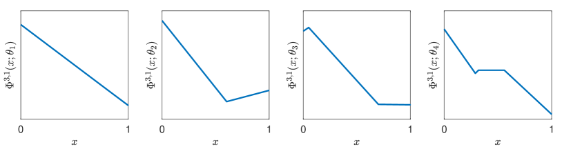
Figure 21: Different outputs of four ReLU networks with a fixed architecture $(W,L)=(3,1)$ and four different parameter sets. Network outputs are piecewise linear functions with up to $W=3$ breakpoints.

To see the first inclusion, we note that every continuous piecewise linear function on $[0,1]$ with $W-1$ interior breakpoints on $(0,1)$ is the restriction of a function from ${\mathcal{M}}_{W,1}$ to $[0,1]$. Indeed, every $S\in{\mathcal{S}}_{W-1}$ on $[0,1]$ with interior breakpoints $x_{1},\dotsc,x_{W-1}$ can be represented by

$$S(x)=a\,x+b+\sum_{j=1}^{W-1}m_{j}\,\sigma(x-x_{j})=\begin{bmatrix}a&m_{1}&\cdots&m_{W-1}\end{bmatrix}\,\sigma\left(\begin{bmatrix}1\\ 1\\ \vdots\\ 1\end{bmatrix}\,x+\begin{bmatrix}0\\ -x_{1}\\ \vdots\\ -x_{W-1}\end{bmatrix}\right)+b,$$

which means $S\in{\mathcal{M}}_{W,1}$. Hence ${\mathcal{S}}_{W-1}\subset{\mathcal{M}}_{W,1}$. As an example, the hat function $H:[0,1]\rightarrow[0,1]$ that has one interior breakpoint belongs to ${\mathcal{M}}_{2,1}$,

$$H(x)=2\sigma(x)-4\sigma(x-0.5).$$

Note that as we have sen before, $H$ belongs to ${\mathcal{M}}_{3,1}$ on ${\mathbb{R}}$, and only its restriction to $[0,1]$ belongs to ${\mathcal{M}}_{2,1}$.

16.4 A comparison between deep ReLU networks and free knot linear splines

The composition of two continuous piecewise linear functions will be another continuous piecewise linear function with the maximum number of breakpoints equal to the product of the number of breakpoints of individual functions. That is, if $f$ has $n$ breakpoints and $g$ has $m$ breakpoints, then $f\circ g$ will have at most $nm$ breakpoints. This allows networks with $L$ hidden layers of width $W$ to create roughly $W^{L}$ breakpoints by $n(W,L)\sim W^{2}L$ special choices of parameters (weights and biases). This means that a “deep” network with $n(W,L)$ parameters can produce functions with many more breakpoints than the number of parameters ($W^{L}\gg W^{2}L$ when $L$ is large). On the other hand, the number of parameters of a free knot spline is roughly double the number of breakpoints ($2n+2\sim 2n$). As we will see in the remainder of this chapter, this gives deep networks approximation superiority over free knot linear splines provided the target function has a special (compositional/self-similarity) structure.

17 ReLU networks are at least as expressive as free knot linear splines

Throughout this section, we fix $W\geq 8$ and let $L\geq 2$ and consider ${\mathcal{M}}_{W,L}$. The goal is to show that ${\mathcal{S}}_{n}\subset{\mathcal{M}}_{W,L}$ where $n(W,L)\leq C\,n$ with an absolute constant $C$. Precisely, we will show that for every fixed $W\geq 8$, any function in ${\mathcal{S}}_{n}$ is the output of a (special) network with the number of parameters comparable to $n$. We extensively use the following quantity

$$q:=\Bigl{\lfloor}\frac{W-2}{6}\Bigr{\rfloor},\qquad W\geq 8.$$ (32)

Theorem 1.

Fix $W\geq 8$ and let $n\geq 1$. The set ${\mathcal{S}}_{n}$ of free knot linear splines with at most $n$ breakpoints is contained in the set ${\mathcal{M}}_{W,L}$, where $L=2$ when $n<q(W-2)$ and $L=2\lceil n/q(W-2)\rceil$ when $n\geq q(W-2)$. The complexity of such network space ${\mathcal{M}}_{W,L}$ is $n(W,L)=W^{2}+4W+1$ when $n<q(W-2)$ and $n(W,L)\leq 61n$ when $n\geq q(W-2)$.

The rest of this section will be devoted to the proof of Theorem 1. The proof is constructive and utilizes a special type of ReLU networks.

17.1 Special ReLU networks

For $W\geq 4$ and $L\geq 2$ we consider a special ReLU network as a “special” subset of a ReLU network with the same width and depth, where special roles are reserved for the top and bottom neurons of hidden layers. Specifically, we define three types of channels for special ReLU networks:

• A source channel formed by top neurons that are assumed to be ReLU-free with unit weights and without any bias. The neurons in a source channel do not take any input from neurons in other channels and do not do any computation. This channel simply carries forward the input $x$.

• A collation channel formed by bottom neurons that are also assumed to be ReLU-free. This channel is used to collect all intermediate computations (i.e. outputs of hidden layers). The neurons in a collation channel do not feed into subsequent calculations. They only take outputs of neurons in previous layer and carry them over with unit weight to subsequent bottom neurons.

• The rest of channels are regular computational channels.

Figure 22 displays the graph representation of a special ReLU network with $W=4$ and $L=3$.

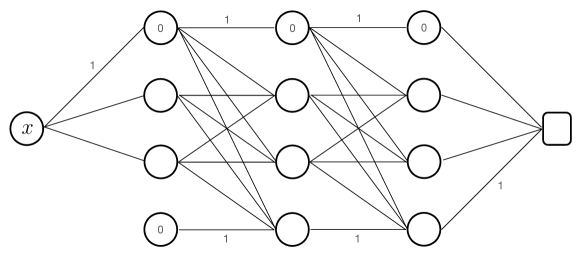
Figure 22: Graph representation of a special ReLU network in $\hat{\mathcal{M}}_{4,3}$.

We denote by $\hat{\mathcal{M}}_{W,L}$ the set of all functions generated by special ReLU networks,

$$\hat{\mathcal{M}}_{W,L}=\{\Phi:[0,1]\rightarrow{\mathbb{R}}\ \ \text{produced by a special network of width $W\geq 4$ and depth $L\geq 2$}\}.$$

It is to be noted that since top and bottom neurons are ReLU free, special networks do not form a direct subset of ReLU networks. However, we make the following observations:

• Since the input is non-negative, $x\in[0,1]$, then $x=\sigma(x)$, and hence the assumption that top neurons are ReLU free is not restrictive.

• The first bottom neuron in the first hidden layer ($\ell=0$) is simply taking zero and since $0=\sigma(0)$, the ReLU free assumption is not restrictive.

• Any other bottom neuron in the remaining $L-1$ hidden layers ($\ell=1,\dotsc,L-1$) takes an input function, say $g_{\ell}(x)$ that depends continuously on $x$. Hence there is a constant, say $C_{\ell}$, such that $g_{\ell}(x)+C_{\ell}\geq 0$ for every $x\in[0,1]$. This implies that $g_{\ell}(x)=\sigma(g_{\ell}(x)+C_{\ell})-C_{\ell}$.

Consequently, given any function $\Phi\in\hat{\mathcal{M}}_{W,L}$, determined by the parameter set $\{\hat{W}^{(\ell)},\hat{b}^{(\ell)}\}_{\ell=0}^{L}$, one can construct a ReLU network with the same complexity that produces the same function $\Phi$. The parameters $\{{W}^{(\ell)},{b}^{(\ell)}\}_{\ell=0}^{L}$ of such ReLU network are given in terms of the parameters of the special network by

$${W}^{(\ell)}=\hat{W}^{(\ell)},\qquad\ell=0,\dotsc,L,$$

$$b_{j}^{(\ell)}=\hat{b}_{j}^{(\ell)},\qquad j=1,\dotsc,W-1,\qquad b_{W}^{(\ell)}=\hat{b}_{W}^{(\ell)}+C_{\ell},\qquad\ell=1,\dotsc,L-1,$$

$$b^{L}=\hat{b}^{L}-\sum_{\ell=1}^{L-1}C_{\ell}.$$

This implies that given any $\Phi\in\hat{\mathcal{M}}_{W,L}$, there exists a standard ReLU network in ${\mathcal{M}}_{W,L}$ with the same complexity that produces $\Phi$. Hence, although special networks are not direct subsets of ReLU networks, in terms of sets of functions produced by them the following inclusion holds,

$$\hat{\mathcal{M}}_{W,L}\subset{\mathcal{M}}_{W,L}.$$

Proposition 3.

Special ReLU networks have the following properties:

• For every $\ W,L_{1},L_{2}:\qquad\hat{\mathcal{M}}_{W,L_{1}}+\hat{\mathcal{M}}_{W,L_{2}}\subset\hat{\mathcal{M}}_{W,L_{1}+L_{2}}$.

• For $L<P:\ \ \ \hat{\mathcal{M}}_{W,L}\subset\hat{\mathcal{M}}_{W,P}$.

Proof.

We first prove (i). Fix two networks/functions $\Phi_{1}\in\hat{\mathcal{M}}_{W,L_{1}}$ and $\Phi_{2}\in\hat{\mathcal{M}}_{W,L_{2}}$, and construct a concatenated network as follows.

• Start by placing the input and all $L_{1}$ hidden layes of $\Phi_{1}$;

• Continue with placing the first hidden layer of $\Phi_{2}$ with one change: in its collation neuron place the output of $\Phi_{1}$ rather than zero;

• Finally, place the remaining hidden layers and output layer of $\Phi_{2}$.

The output of such concatenated network, which has $L_{1}+L_{2}$ hidden layers, will be $\Phi_{1}+\Phi_{2}$ as desired, thanks to the concatenated collation channel that carries over $\Phi_{1}$ and adds it to $\Phi_{2}$; see Figure 23.

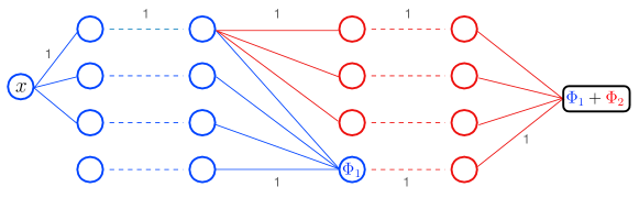
Figure 23: Graph representation of the concatenated network that outputs the sum of $\Phi_{1}$ (in blue) and $\Phi_{2}$ (in red).

Proof of (ii) follows from (i) with $\Phi_{2}\equiv 0$ and $L_{1}=L$ and $L_{2}=P-L$.

∎

17.2 Special ReLU networks that realize continuous piecewise linear functions

Consider a positive integer $M=q(W-2)$, with $q$ in (32). Note that since $q$ is of order of $W$, the integer $M$ will be of order of $W^{2}$ and may hence be a small number. We first show how to construct a special ReLU network with only 2 hidden layers that generates continuous piecewise linear functions with $M$ (that may be small) breakpoints.

Let $x_{1}<\dotsc<x_{M}\in(0,1)$ be any $M$ given breakpoints in the interior of $[0,1]$. Let $x_{0}=0$ and $x_{M+1}=1$. Let further ${\mathcal{S}}_{M}^{0}={\mathcal{S}}_{M}^{0}(x_{0},x_{1},\dotsc,x_{M+1})$ denote the set of all continuous piecewise linear functions that vanish outside $(0,1)$ and with breakpoints only at $x_{0},x_{1},\dotsc,x_{M+1}$. The space ${\mathcal{S}}_{M}^{0}$ is a linear space of dimension $M$ (and not $M+2$ because its elements vanish at $x_{0}$ and $x_{M+1}$).

Lemma 6.

For every $M$ breakpoints $x_{1}<\dotsc<x_{M}\in(0,1)$, where $M=q(W-2)$, with $q$ in (32), we have

$${\mathcal{S}}_{M}^{0}\subset\hat{\mathcal{M}}_{W,2}.$$

Proof.

Step 1. We first create a particular basis for ${\mathcal{S}}_{M}^{0}$ as follows. We introduce a set $\{\xi_{j}=x_{jq}\}_{j=1}^{W-2}$ of $W-2$ “principal breakpoints”, where each $\xi_{j}$ is associated with $q$ hat basis functions $H_{i,j}$, $i=1,\dotsc,q$, that take value 1 at $\xi_{j}$ and are supported on $[x_{jq-i},x_{jq+1}]$; see Figure 24.

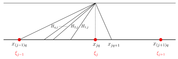
Figure 24: Schematic representation of $q$ basis hat functions $H_{1,j},\dotsc,H_{q,j}$ associated to the principle breakpoint $\xi_{j}$.

We notice that the case $q=1$ (when $8\leq W\leq 13$) simply coincides with the familiar finite element basis with Lagrange elements. There will be a total number of $M$ basis function, and we name them $\{\phi_{k}\}_{k=1}^{M}$, ordered in such a way that $\phi_{k}$ has leftmost breakpoint $x_{k-1}$. We say $\phi_{k}$ is associated with $\xi_{j}$ if $\phi_{k}(\xi_{j})=1$. Clearly, $\{\phi_{k}\}_{k=1}^{M}$ forms a basis for ${\mathcal{S}}_{M}^{0}$, as $\phi_{k}$’s are linearly independent. Indeed, if $\sum_{k=1}^{M}c_{k}\,\phi_{k}=0$, then $c_{1}=0$ because $\phi_{1}$ is the only nonzero function on $[x_{0},x_{1}]$. With a similar argument, considering $\phi_{2}$, we get $c_{2}=0$, etc.

Step 2. Let $S\in{\mathcal{S}}_{M}^{0}$. By Step 1, we can write $S(x)=\sum_{k=1}^{M}c_{k}\,\phi_{k}(x)$. Note that with principal breakpoints $\xi_{1},\dotsc,\xi_{W-2}$, we have $S(\xi_{j})=\sum_{k:\phi_{k}(\xi_{j})=1}c_{k}$, and there are $q$ indices in the summation associated to each principal breakpoint. We take the index set $\Lambda=\{1,\dotsc,M\}$ and divide it into two sets $\Lambda=\Lambda^{+}\cup\Lambda^{-}$, where

$$\Lambda^{+}=\{k\in\Lambda:\ c_{k}\geq 0\},\qquad\Lambda^{-}=\{k\in\Lambda:\ c_{k}<0\}.$$

We then divide each of $\Lambda^{+}$ and $\Lambda^{-}$ into at most $3q$ subsets. For instance, we split $\Lambda^{+}$ into

$$\Lambda_{i,m}^{+}=\{s\in\Lambda^{+}:\ \phi_{s}=H_{i,j}\ \ \text{such that}\ \ j\ \text{mod}\ 3=m\},\qquad i=1,\dotsc,q,\ \ \ m=0,1,2.$$

More explicitly, we get three sets

$$\Lambda_{i,0}^{+} =\{s\in\Lambda^{+}:\ \phi_{s}=H_{i,3}\ \text{or}\ \phi_{s}=H_{i,6}\ \text{or}\ \phi_{s}=H_{i,9}\ \dotsc\}$$

$$\Lambda_{i,1}^{+} =\{s\in\Lambda^{+}:\ \phi_{s}=H_{i,1}\ \text{or}\ \phi_{s}=H_{i,4}\ \text{or}\ \phi_{s}=H_{i,7}\ \dotsc\}$$

$$\Lambda_{i,2}^{+} =\{s\in\Lambda^{+}:\ \phi_{s}=H_{i,2}\ \text{or}\ \phi_{s}=H_{i,5}\ \text{or}\ \phi_{s}=H_{i,8}\ \dotsc\}.$$

Similarly, we split $\Lambda^{-}$ into at most $3q$ subsets,

$$\Lambda_{i,m}^{-}=\{s\in\Lambda^{-}:\ \phi_{s}=H_{i,j}\ \ \text{such that}\ \ j\ \text{mod}\ 3=m\},\qquad i=1,\dotsc,q,\ \ \ m=0,1,2.$$

We can hence write $\Lambda=\{1,\dotsc,M\}$ as a disjoint union of $K\leq 6q\leq W-2$ sets $\Lambda_{p}$:

$$\Lambda=\cup_{p=1}^{K}\Lambda_{p},$$

where each $\Lambda_{p}$ has two properties: 1) all coefficients $c_{k}$ of $S$ with $k\in\Lambda_{p}$ have the same sign, and 2) for every $k,k^{\prime}\in\Lambda_{p}$, the associated principle breakpoints $\xi_{j}$ and $\xi_{j^{\prime}}$ (associated to $\phi_{k}$ and $\phi_{k^{\prime}}$) satisfy the separation/non-overlapping property $|j-j^{\prime}|\geq 3$. We note that some of $\Lambda_{p}$’s may be empty, and hence we may get $K<W-2$. In this case we set $\Lambda_{K+1}=\dotsc=\Lambda_{W-2}=\emptyset$. We then write

$$S(x)=\sum_{p=1}^{W-2}S_{p}(x),\qquad S_{p}=\left\{\begin{array}[]{l l}\sum_{i\in\Lambda_{p}}c_{i}\,\phi_{i}(x),&\qquad\Lambda_{p}\neq\emptyset,\\ 0,&\qquad\Lambda_{p}=\emptyset.\end{array}\right.$$ (33)

Because of the separation property, all $\phi_{i}$’s with $i\in\Lambda_{p}$ have disjoint supports, and hence $c_{i}=S_{p}(\xi_{j})$, where $\xi_{j}$ is the principal breakpoint associated to $\phi_{i}$.

Step 3. We next show that each $S_{p}$ corresponding to a nonempty $\Lambda_{p}$ is of the form $\pm\sigma(g_{p}(x))$, where $g_{p}$ is a continuous piecewise linear function whose breakpoints are the principal breakpoints $\xi_{1},\dotsc\xi_{W-2}$. We fix $p$ and first consider the case where all $c_{i}$’s in $\Lambda_{p}$ are non-negative. We let $g_{p}$ be the continuous piecewise linear function that takes the value $c_{i}$ at each principal breakpoint $\xi_{j}$ associated to $i\in\Lambda_{p}$. Note that each $i\in\Lambda_{p}$ has a different associated $\xi_{j}$ thanks to the separation property. At the remaining principal breakpoints, we assign negative values for $g_{p}$ such that $g_{p}$ vanishes at the leftmost and rightmost breakpoints of all $\phi_{i}$’s with $i\in\Lambda_{p}$. Again, this is possible thanks to the separation property. A simple example is depicted in Figure 25. It follows that $\sigma(g_{p}(x))=S_{p}(x)$. Similarly, when all $c_{i}$’s in $\Lambda_{p}$ are negative, we will do a similar procedure noting that $-\sigma(-g_{p}(x))=S_{p}(x)$.

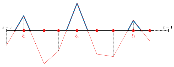
Figure 25: A simple example of constructing $g_{p}$ (thin red line) such that $\sigma(g_{p}(x))=S_{p}(x)$. The function $S_{p}$ is displayed with thick blue line. Clearly, $g_{p}$ is a continuous piecewise linear function whose breakpoints are the principal breakpoints $\xi_{1},\dotsc\xi_{W-2}$ (red circles). Note that $g_{p}$ vanishes at the leftmost and rightmost breakpoints (black circles) of all $\phi_{i}$’s with $i\in\Lambda_{p}$.

Step 4. Finally, we construct a special ReLU network with two hidden layers that generates $S(x)=\sum_{p=1}^{W-2}S_{p}(x)$; see Figure 26.

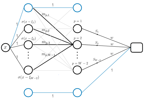
Figure 26: A special ReLU network with two hidden layers that outputs $S(x)=\sum_{p=1}^{W-2}S_{p}(x)$.

The $W-2$ compute neurons labeled $j=1,\dotsc,W-2$ in the first hidden layer are used to generate $\sigma(x-\xi_{j})$, with $j=1,\dotsc,W-2$. This can be easily done by setting input weights to 1 and biases to $\xi_{1},\dotsc,\xi_{W-2}$. In the second hidden layer, each compute unit, labeled $p=1,\dotsc,W-2$, is used to take $x$ and all $\sigma(x-\xi_{j})$’s with $j=1,\dotsc,W-2$ to output $S_{p}$. To find the corresponding weights and biases, we first note that the index $p=1,\dotsc,W-2$ corresponds to a different labeling of the index set $\{(i,m,\pm),\ i=1,\dotsc,q,\ m=0,1,2\}$. Each $p$ corresponds to a triplet $(i,m,+)$ or $(i,m,-)$. We take a fixed $p$, say corresponding to $(i,m,+)$, and this gives us the set $\Lambda_{i,m}^{+}$ which corresponds to the set $\Lambda_{p}$ which in turn contains indices $i\in\Lambda_{p}$ in $S_{p}(x)=\sum_{i\in\Lambda_{p}}c_{i}\,\phi_{i}(x)=\sigma(g_{p}(x))$. All we will need to do is to find the weights $\{m_{p,1},\dotsc,m_{p,W-1}$ and the bias $b_{p}$ in the second hidden layer such that

$$g_{p}(x)=m_{p,1}x+\sum_{j=2}^{W-1}m_{p,j}\,\sigma(x-\xi_{j-1})+b_{p}.$$

This can be easily done recalling that $g_{p}$ is a continuous piecewise linear function whose breakpoints are the principal breakpoints $\xi_{1},\dotsc\xi_{W-2}$, and hence it can be represented by a linear combination of $\{\sigma(x-\xi_{j})\}_{j=1}^{W-2}$ and $x$ terms. To do this we start with noting that $b_{p}=g_{p}(0)$. Then we take the first principal breakpoints and write $g_{p}(\xi_{1})=m_{p,1}\,\xi_{1}+b_{p}$, which gives us $m_{p,1}$. Then we proceed with the second principal breakpoints and write $g_{p}(\xi_{2})=m_{p,1}\,\xi_{2}+m_{p,2}\,(\xi_{2}-\xi_{1})+b_{p}$, which gives us $m_{p,2}$, and so forth. We note that in this particular setup, the source and collation channels are not used. Nevertheless we keep them in case we would need to performa concatenation or other operations on the input-output. This completes the proof. ∎

We will now focus on the construction of deep special ReLU networks with many hidden layers that generate continuous piecewise linear functions with a large number of breakpoints.

Lemma 7.

For every $N$ breakpoints $x_{1}<\dotsc<x_{N}\in(0,1)$, where $N=q(W-2)L$, with $q$ in (32), we have

$${\mathcal{S}}_{N}\subset\hat{\mathcal{M}}_{W,2L}.$$

Proof.

We need to show that every $S\in{\mathcal{S}}_{N}$ is the output of a special ReLU network with width $W$ and depth $2L$. Let $x_{1}<\dotsc<x_{N}$ be the breakpoints of $S$ in $(0,1)$, and set $x_{0}=0$ and $x_{N+1}=1$. Let $g(x)=ax+b$ be the linear function that interpolates $S$ at the two endpoints 0 and 1. Then $T=S-g\in{\mathcal{S}}_{N}^{0}$ vanishes at the endpoints, and it will be enough to show that $T\in\hat{\mathcal{M}}_{W,2L}$. We first write $T=T_{0}+T_{1}+\dotsc+T_{L-1}$, where each $T_{j}\in{\mathcal{S}}_{N}^{0}$ is a continuous piecewise linear function that agrees with $T$ at the points $\{x_{jq(W-2)+1},\dotsc,x_{(j+1)q(W-2)}\}$ and is zero at all other breakpoints of $T$; see an example in Figure 27.

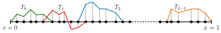
Figure 27: Decomposition of $T=T_{0}+T_{1}+\dotsc+T_{L-1}\in{\mathcal{S}}_{N}^{0}$ into $L$ functions $T_{j}\in{\mathcal{S}}_{M}^{0}$, with $j=0,1,\dotsc,L-1$, where $N=ML$.

Since each $T_{j}$ may be non-zero only at $M=q(W-2)$ breakpoints, we will have $T_{j}\in{\mathcal{S}}_{M}^{0}$ for $j=0,1,\dotsc,L-1$. By Lemma 6 we have $T_{j}\in\hat{\mathcal{M}}_{W,2}$, with $j=0,1,\dotsc,L-1$. We can now simply concatenate these $L$ networks as in Proposition 3 and construct a network with $2L$ hidden layers that realizes $T$. Finally, in order to produce $S=T+g$, where $g(x)=ax+b$, we can simply use the source channel and assign weight $a$ to the link the top neuron of the last hidden layer and the output neuron (which was not used when generating $T_{L-1}$). We also assign bias $b$ to the output neuron. This complete the proof. ∎

17.3 Proof of Theorem 1

We need to show that ${\mathcal{S}}_{n}\subset{\mathcal{M}}_{W,L}$ where $n(W,L)\sim n$. By Lemma 7 and inclusion $\hat{\mathcal{M}}_{W,2L}\subset{\mathcal{M}}_{W,2L}$, we have

$${\mathcal{S}}_{N}\subset{\mathcal{M}}_{W,2L},\qquad N=ML,\qquad M=q\,(W-2),$$ (34)

with $q$ given in (32). We consider two cases.

If $n<M$, then we have ${\mathcal{S}}_{n}\subset{\mathcal{S}}_{M}\subset{\mathcal{M}}_{W,2}$, where the second inclusion follows from (34) with $L=1$. Clearly we have $n(W,2)=2W(W+1)-(W-1)^{2}+2=W^{2}+4W+1$ as desired.

If $n\geq M$, we choose

$$L=\lceil\frac{n}{q(W-2)}\rceil<\frac{n}{q(W-2)}+1,$$

and hence

$$n(W,2L) =2LW(W+1)-(W-1)^{2}+2$$

$$<2W(W+1)(1+n/q(W-2))-(W-1)^{2}+2$$

$$=\frac{2W(W+1)}{q(W-2)}n+W^{2}+4W+1$$

$$<34n+W^{2}+4W+1.$$

The last inequality is because $2W(W+1)/q(W-2)$ attains its maximum for $W=13$ and $q=1$, and hence $2W(W+1)/q(W-2)\leq 364/11<34$. Moreover, it is easy to see that by (32) we have $W^{2}+4W+1<27q(W-2)\leq 27n$. Hence we get $n(W,2L)<34n+27n=61n$, as desired. This completes the proof of Theorem 1. ∎

18 The power of depth

So far we have seen that ReLU networks are at last as expressiv as free knot linear splines with at most $n$ breakpoints. Similar results also hold when comparing ReLU networks with other nonlinear approximation methods; see e.g. Section 6 of [7] that comapres ReLU networks with $n$-term approximation from a Fourier-like basis.

In this section we will discuss the power of depth. Precisely, we show that there exists a large class of functions that possess self-similarity and hence can be approximated by ReLU networks with approximation rates that far exceed the approximation rates of free knot linear splines or any other classical approximation family.

We will first present a few additive and compositional properties of standard and special ReLU networks (see Section 18.1) and then utilize them to discuss and exemplify the power of depth for self-similar functions (see Section 18.2).

18.1 Additive and compositional properties of ReLU networks

Proposition 4.

Let $W\geq 2$. For any $\Phi_{j}\in{\mathcal{M}}_{W,L_{j}}$ with $j=1,\dotsc,J$, the followings hold:

• $\Phi_{J}\circ\dotsc\circ\Phi_{1}\in{\mathcal{M}}_{W,L_{1}+\dotsc+L_{J}}$.

• $\Phi_{1}+\dotsc+\Phi_{J}\in\hat{\mathcal{M}}_{W+2,L_{1}+\dotsc+L_{J}}$.

Proof.

To prove (i), we first concatenate the networks $\Phi_{1}$ and $\Phi_{2}$ as follows to construct a network, say $\Phi_{2\circ 1}$, that outputs $\Phi_{2}\circ\Phi_{1}$:

1. The input and the first $L_{1}$ hidden layers of $\Phi_{2\circ 1}$ will be the same as the input and $L_{1}$ hidden layers of $\Phi_{1}$.

2. The ($L_{1}+1$)-st hidden layer of $\Phi_{2\circ 1}$ the first hidden layer of $\Phi_{2}$.

3. The weights between hidden layers $L_{1}$ and $L_{1}+1$ (a $W\times W$ matrix) will be the output weights of $\Phi_{1}$ (a $1\times W$ vector) multiplied from left by the input weights of the first hidden layer of $\Phi_{1}$ (a $W\times 1$ vector).

4. The bias of hidden layer $L_{1}+1$ will be the bias of the first hidden layer of $\Phi_{2}$ plus the product of the output bias of $\Phi_{1}$ and the input weights of the first hidden layer of $\Phi_{2}$.

5. The remaining hidden layers of $\Phi_{2\circ 1}$ will be the same as the remaining hidden layers of $\Phi_{2}$.

The resulting network will have $L_{1}+L_{2}$ hidden layers. This procedure can be applied $J-1$ times to generate $\Phi_{J\circ\dotsc\circ 1}$ with $L_{1}+\dotsc+L_{J}$ hidden layers.

To prove (ii), we concatenate the standard ReLU networks $\Phi_{1}$ and $\Phi_{2}$ by adding a source and a collation channel, as shown in Figure 28, to construct a special ReLU network, say $\Phi_{1+2}$, with width $W+2$ and depth $L_{1}+L_{2}$, that outputs $\Phi_{1}+\Phi_{2}$. Again this can be repeated $J-1$ times to build a network with width $W+2$ and depth $L_{1}+\dotsc+L_{J}$ that outputs $\Phi_{1}+\dotsc+\Phi_{J}$. This completes the proof.

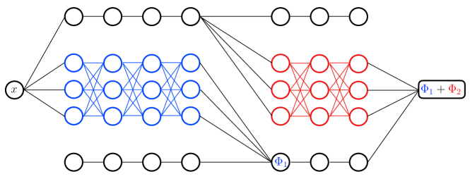
Figure 28: By adding source and collation channels we can concatenate two standard ReLU networks $\Phi_{1}$ (in blue) and $\Phi_{2}$ (in red) and generate a special ReLU network that outputs $\Phi_{1}+\Phi_{2}$.

∎

In what follows, we denote by $g^{\circ k}$ the $k$-fold composition of a function $g$ with itself

$$g^{\circ k}(x)=\underbrace{{g\circ g\circ\dotsc\circ g}}_{k\,\,\text{times}}(x),\qquad s\geq 1.$$

Note that $g^{\circ 1}(x)=g(x)$.

Proposition 5.

Let $W\geq 2$. For any $T\in{\mathcal{M}}_{W,L}$, then

$$\Phi(x)=\sum_{i=1}^{m}a_{i}\,T^{\circ i}(x)\in\hat{\mathcal{M}}_{W+2,mL}.$$

Proof.

We first generate $T^{\circ m}(x)$ as discussed in the proof of Proposition 4 (i), displayed in blue and red in Figure 29. We add a collation channel and modify the input weights (displayed in green) of every $i$-th output collation neuron so that it produces $a_{i}\,T^{\circ i}(x)$. The source channel is not needed in this case. Nevertheless, we include it in case we need to add another function of $x$ to $\Phi$ later on.

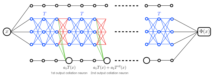
Figure 29: Concatenation of $m$ standard ReLU networks, each generating the same function $T$, and addition of a collation channel to output $\Phi(x)=\sum_{i=1}^{m}a_{i}\,T^{\circ i}(x)$.

∎

Proposition 6.

Let $W\geq 2$. For any $T\in{\mathcal{M}}_{W_{1},L}$ and $g\in{\mathcal{M}}_{W_{2},L}$, then

$$\Phi_{g}(x)=\sum_{i=1}^{m}a_{i}\,g\circ T^{\circ i}(x)\in\hat{\mathcal{M}}_{W_{1}+W_{2}+2,(m+1)L}.$$

Proof.

The construction of $\Phi_{g}$ is similar to the construction of $\Phi$ in Proposition 5 with the extra step of adding $m$ copies of $g$ to $T^{\circ m}$ as depicted in Figure 30.

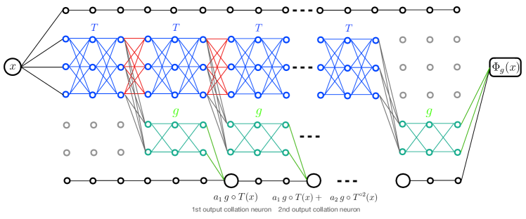
Figure 30: Concatenation of $m$ standard ReLU networks, each generating the same function $g\circ T$, and addition of a collation channel to output $\Phi_{g}(x)=\sum_{i=1}^{m}a_{i}\,g\circ T^{\circ i}(x)$.

∎

18.2 A large class of functions with self-similarity

Consider target functions of the form

$$f(x)=\sum_{k\geq 1}a^{-k}\,g\circ T^{\circ k}(x),\qquad|a|>1,\qquad g:[0,1]\rightarrow{\mathbb{R}},\qquad T:[0,1]\rightarrow[0,1].$$

This is an example of a self-similar function. By Proposition 6, if

$$T\in{\mathcal{M}}_{W_{1},L},\qquad g\in{\mathcal{M}}_{W_{2},L},$$

then

$$\Phi_{m}(x)=\sum_{k=1}^{m}a^{-k}\,g\circ T^{\circ k}(x)\ \in\ \hat{\mathcal{M}}_{W,(m+1)L},\qquad W=W_{1}+W_{2}+2.$$

We now define the (best) approximation error in approximating $f$ by special ReLU networks with a fixed width $W$ and depth $(m+1)L$ by

$$\varepsilon_{(m+1)L}(f)_{C[0,1]}:=\inf_{\Phi\in\hat{\mathcal{M}}_{W,(m+1)L}}||f-\Phi||_{C[0,1]}.$$

Assuming $||g||_{C[0,1]}=1$ (this can easily be relaxed), then we will have

$$\varepsilon_{(m+1)L}(f)_{C[0,1]} \leq||f-\Phi_{m}||_{C[0,1]}$$

$$=||\sum_{k>m}a^{-k}\,g\circ T^{\circ k}||_{C[0,1]}$$

$$\leq\sum_{k>m}|a|^{-k}\,||g\circ T^{\circ k}||_{C[0,1]}$$

$$=|a|^{-(m+1)}\,\left(1+\sum_{k>m+1}|a|^{-k}\right)\leq C\,|a|^{-(m+1)},$$

where $C<\infty$ is a constant, noting that $\sum_{k\geq 0}|a|^{-k}=1/(1-|a|^{-1})$. We note that the second inequality is a simple consequence of triangle inequality. The above estimate implies that the target function $f$ can be approximated by a ReLU network with exponential accuracy (i.e. the approximation error decays exponentially). Moreover, the deeper the network, that is, the more terms $m$ in the sum, the higher the exponential rate of decay.

We now consider a special class of such self-similar functions, known as Takagi functions, and present two examples of Takagi functions showing that they form a large class of functions that can be well approximated by deep ReLU networks.

Takagi functions. Consider continuous functions of the form

$$f(x)=\sum_{k\geq 1}a_{k}\,H^{\circ k}(x),$$ (35)

where $\{a_{k}\}_{k\geq 1}$ is an absolutely summable sequence of real numbers, and $H\in{\mathcal{M}}_{2,1}$ is the hat function. Note that this is a self-similar function with $g(x)=x$ and $T(x)=H(x)$. By Proposition 4(i), we will have $H^{\circ k}\in{\mathcal{M}}_{2,k}$. Following Proposition 5, a special ReLU network approximating any Takagi function of the form (35) can be easily constructed; see Figure 31.

Figure 31: A special ReLU network with width $W=4$ and $L$ hidden layers that outputs $\Phi_{L}(x)=\sum_{k=1}^{L}a_{k}\,H^{\circ k}(x)$, approximating a Takagi function $\Phi(x)=\sum_{k\geq 1}a_{k}\,H^{\circ k}(x)$. The deeper the network, the higher the rate of decay in approximation error.

The depth $L$ of such special ReLU network, which is equal to the number of terms in the approximant $\Phi_{L}(x)=\sum_{k=1}^{L}a_{k}\,H^{\circ k}(x)$, will determine the exponential decay rate of approximation error. We will give two specific examples.

Example 1. Consider a Takagi function (35) with $a_{k}=2^{-k}$,

$$f_{1}(x)=\sum_{k\geq 1}2^{-k}\,H^{\circ k}(x).$$

Let $\Phi_{L}(x)=\sum_{k=1}^{L}2^{-k}\,H^{\circ k}(x)$ be the ReLU network approximant of $f_{1}$, with depth $L\geq 1$. Then, by the error estimate obtained above, we will have

$$\varepsilon_{L}(f_{1})_{C[0,1]}\leq C\,2^{-L}.$$

This implies that theoretically $f_{1}$ can be approximated with exponential accuracy by ReLU networks with roughly $W^{2}L\sim L$ parameters (noting that $W=4$ in the above construction). This reveals an amazing power of deep networks, as $f_{1}$ is nowhere differentiable and hence has very little smoothness in classical sense. In fact, all traditional methods of approximation would fail to approximate $f_{1}$ well. The key to the success of deep network is however the self-similarity feature of $f_{1}$; it possesses a simple compositional/recursive pattern that can be exploited by deep networks.

Example 2. Consider a Takagi function (35) with $a_{k}=4^{-k}$,

$$f_{2}(x)=\sum_{k\geq 1}4^{-k}\,H^{\circ k}(x)=x(1-x).$$

Unlike $f_{1}$ which has very little smoothness, $f_{2}$ is an analytic (very smooth) function. This representation can be used to show that the quadratic function $x^{2}$ can be approximated with exponential accuracy by ReLU networks (as we did earlier). We can then show that all monomials $x^{3},x^{4},\dotsc$ can also be approximated with exponential accuracy by ReLU networks. Using the additive property of ReLU networks, discussed in Section 18.1, we can conclude that analytic functions (and Sobolev functions) can be approximated by ReLU networks with the same accuracy as their approximation by algebraic polynomials (a result that we obtained in previous chapter).

A concluding remark. The above two examples show that the approximation space of deep ReLU networks is quite large. It contains many functions, spanning from smooth/analytic functions to functions that are not smooth in any classical sense. This brings flexibility to deep ReLU networks: they well approximate functions with little classical smoothness and retain the good property of approximating smooth functions with comparable accuracy to other methods of approximation.

 

Acknowledgments. This survey is mainly based on two courses on “Mathematics of deep learning” that the author designed and gave at The University of New Mexico in Fall 2021 and at Uppsala University, Sweden, in Spring 2022. The author would like to thank all students and researchers who actively participated in class and colleagues and collaborators who contributed to the survey through interesting discussions. The author is also indebted to Gunilla Kreiss for the support she provided during a one-month visit to Uppsala University.

References

- [1] A. R. Barron. Universal approximation bounds for superpositions of a sigmoidal function. IEEE Trans. Inform. Theory, 39:930–945, 1993.
- [2] Y. Bengio. Practical recommendations for gradient-based training of deep architectures. In Müller KR. Montavon G., Orr G.B., editor, Neural Networks: Tricks of the Trades, pages 437–478. Springer, Berlin, 2012.
- [3] Alberto Bietti, Luca Venturi, and Joan Bruna. On the sample complexity of learning under geometric stability. In A. Beygelzimer, Y. Dauphin, P. Liang, and J. Wortman Vaughan, editors, Advances in Neural Information Processing Systems, 2021.
- [4] L. Bottou, F. E. Curtis, and J. Nocedal. Optimization methods for large-scale machine learning. SIAM Rev., 60:223–311, 2018.
- [5] S. C. Brenner and L. R. Scott. The Mathematical Theory of Finite Element Methods. Springer, 2008.
- [6] C. Canuto, M. Y. Hussaini, A. Quarteroni, and T. A. Zang. Spectral Methods: Fundamentals in Single Domains. Springer, 2006.
- [7] I. Daubechies, R. DeVore, S. Foucart, B. Hanin, and G. Petrova. Nonlinear approximation and (deep) ReLU networks. (accepted/in press). Constructive Approximation, 2021.
- [8] R. A. DeVore. Nonlinear approximation. Acta Numer., 7:51–150, 1998.
- [9] R. A. DeVore and G. G. Lorentz. Constructive Approximation. Springer-Verlag, 1991.
- [10] W. F. Donoghue. Distributions and Fourier Transforms. Academic Press, Inc., New York, 1969.
- [11] W. E, C. Ma, S. Wojtowytsch, and L. Wu. Towards a mathematical understanding of neural network-based machine learning: What we know and what we don’t. CSIAM Trans. Appl. Math., 1:561–615, 2020.
- [12] D. Elbrächter, D. Perekrestenko, P. Grohs, and H. Bölcskei. Deep neural network approximation theory. arxiv:1901.02220, 2021.
- [13] L. C. Evans. Partial Differential Equations, volume 19 of Graduate Studies in Mathematics. American Mathematical Society, Providence, Rhode Island, 1998.
- [14] I. J. Goodfellow, Y. Bengio, and A. Courville. Deep Learning. MIT Press, Cambridge, MA, USA, 2016.
- [15] I. Gühring, G. Kutyniok, and P. Petersen. Error bounds for approximations with deep ReLU neural networks in norms. Analysis and Applications, 18:803–859, 2020.
- [16] J. Kiefer and J. Wolfowitz. Stochastic estimation of the maximum of a regression function. Ann. Math. Statist., 23:462–466, 1952.
- [17] D. P. Kingma and J. Ba. Adam: A method for stochastic optimization. arXiv:1412.6980v9, 2017.
- [18] V. Maiorov and R. Meir. On the near optimality of the stochastic approximation of smooth functions by neural networks. Advances in Computational Mathematics, 13:79–103, 2000.
- [19] Y. Makovoz. Random approximants and neural networks. Journal of Approximation Theory, 85:98–109, 1996.
- [20] H. Mhaskar and T. Poggio. Deep vs. shallow networks: an approximation theory perspective. Analysis and Applications, 14:829–848, 2016.
- [21] H. N. Mhaskar. Neural networks for optimal approximation of smooth and analytic functions. Neural Computation, 8:164–177, 1996.
- [22] P. Petersen and F. Voigtländer. Optimal approximation of piecewise smooth functions using deep ReLU neural networks. Neural Networks, 108:296–330, 2018.
- [23] A. Pinkus. Approximation theory of the MLP model in neural networks. Acta Numer., 8:143–195, 1999.
- [24] T. Poggio, H. Mhaskar, L. Rosasco, B. Miranda, and Q. Liao. Why and when can deep-but not shallow-networks avoid the curse of dimensionality: a review. International Journal of Automation and Computing, 14:503–519, 2017.
- [25] M. J. D. Powell. Approximation Theory and Methods. Cambridge University Press, 1996.
- [26] H. Robbins and S. Monro. A stochastic approximation method. Ann. Math. Statist., 22:400–407, 1951.
- [27] D. E. Rumelhart, G. E. Hinton, and R. J. Williams. Learning representations by back-propagating errors. Nature, 323:533–536, 1986.
- [28] N. Srivastava, G. Hinton, A. Krizhevsky, I. Sutskever, and R. Salakhutdinov. Dropout: A simple way to prevent neural networks from overfitting. Journal of Machine Learning Research, 15:1929–1958, 2014.
- [29] M. Telgarsky. Representation benefits of deep feedforward networks. arxiv:1509.08101, 2015.
- [30] L. N. Trefethen. Approximation Theory and Approximation Practice, Extended Edition. SIAM, 2019.
- [31] D. Yarotsky. Error bounds for approximations with deep ReLU networks. Neural Networks, 94:103–114, 2017.