A coherence parameter characterizing generative compressed sensing with Fourier measurements

Abstract

In [1], a mathematical framework was developed for compressed sensing guarantees in the setting where the measurement matrix is Gaussian and the signal structure is the range of a generative neural network (GNN). The problem of compressed sensing with GNNs has since been extensively analyzed when the measurement matrix and/or network weights follow a subgaussian distribution. We move beyond the subgaussian assumption, to measurement matrices that are derived by sampling uniformly at random rows of a unitary matrix (including subsampled Fourier measurements as a special case). Specifically, we prove the first known restricted isometry guarantee for generative compressed sensing (GCS) with subsampled isometries and provide recovery bounds, addressing an open problem of [2, p. 10]. Recovery efficacy is characterized by the coherence, a new parameter, which measures the interplay between the range of the network and the measurement matrix. Our approach relies on subspace counting arguments and ideas central to high-dimensional probability. Furthermore, we propose a regularization strategy for training GNNs to have favourable coherence with the measurement operator. We provide compelling numerical simulations that support this regularized training strategy: our strategy yields low coherence networks that require fewer measurements for signal recovery. This, together with our theoretical results, supports coherence as a natural quantity for characterizing GCS with subsampled isometries.

I Introduction

The solution of underdetermined linear inverse problems has many important applications including geophysics [3, 4] and medical imaging [5, 6]. In particular, compressed sensing permits accurate and stable recovery of signals that are well represented by one of a certain set of structural proxies (e.g., sparsity) [5, 7]. Moreover, this recovery is effected using an order-optimal number of random measurements [7]. In applications like medical imaging [5], the measurement matrices under consideration are derived from a bounded orthonormal system (a unitary matrix with bounded entries), which complicates the theoretical analysis. Furthermore, for such applications one desires a highly effective representation for encoding the images. Developing a theoretical analysis that properly accounts for realistic measurement paradigms and complexly designed image representations is nontrivial in general [1, 7, 8]. For example, there has been much work validating that generative neural networks (GNNs) are highly effective at representing natural signals [9, 10, 11]. In this vein, recent work has shown promising empirical results for compressed sensing with realistic measurement matrices when the structural proxy is a GNN. Other recent work has established recovery guarantees for compressed sensing when the structural proxy is a GNN and the measurement matrix is subgaussian [1]. (See Section I-A for a fuller depiction of related aspects of this problem.) However, an open problem is the following [2, p. 10]:

Open problem (subIso GCS).

A theoretical analysis of compressed sensing when the measurement matrix is structured (e.g., a randomly subsampled unitary matrix) and the signal model proxy is a GNN.

Broadly, we approach a solution to (subIso GCS). as follows. For a matrix $A\in\mathbb{C}^{m\times n}$, a particular GNN architecture $G:\mathbb{R}^{k}\to\mathbb{R}^{n}$ and an unknown signal $x_{0}\in\operatorname{\mathcal{R}}(G)$, the range of $G$, we determine the conditions (on $A,G,x_{0}$, etc.) under which it is possible to approximately recover $x_{0}$ from noisy linear measurements $b=Ax_{0}+\eta$ by (approximately) solving an optimization problem of the form

$$\min_{z\in\mathbb{R}^{k}}\|b-AG(z)\|_{2}.$$ (1)

Above, $\eta\in\mathbb{C}^{m}$ is some unknown corruption. Specifically, we are interested in establishing sample complexity bounds (lower bounds on $m$) for realistic measurement matrices $A$ — where $A$ is an underdetermined matrix randomly subsampled from a unitary matrix. Namely, the rows of $A$ have been sampled uniformly at random without replacement from a unitary matrix $U\in\mathbb{C}^{n\times n}$. We next present a mathematical description of the subsampling of the rows, described similarly to [12, Section 4].

Definition I.1 (subsampled isometry).

Let $2\leq m\leq n<\infty$ be integers and let $U\in\mathbb{C}^{n\times n}$ be a unitary matrix. Let $\theta:=(\theta_{i})_{i\in[n]}$ be an iid Bernoulli random vector: $\theta_{i}\overset{\text{iid}}{\sim}\mathrm{Ber}(m/n)$. Define the set $\mathcal{J}:=\{j:\theta_{j}=1\}$ and enumerate the elements of $\mathcal{J}$ as $j_{1},\ldots,j_{\tilde{m}}$ where $\tilde{m}:=|\mathcal{J}|$ is a binomial random variable with $\operatorname{\mathbb{E}}\tilde{m}=m$. Let $A\in\mathbb{C}^{\tilde{m}\times n}$ be the matrix whose $i$th row is $\frac{\sqrt{n}}{\sqrt{m}}U_{j_{i}},i\in[\tilde{m}]$. We call $A$ an $(m,U)$-subsampled isometry. When there is no risk of confusion we simply refer to $A$ as a subsampled isometry and implicitly acknowledge the existence of an $(m,\theta,U)$ giving rise to $A$.

With $A$ so defined, $A$ is isotropic: $\operatorname{\mathbb{E}}A^{*}A=\sum_{i=1}^{n}U_{i}^{*}U_{i}=I_{n}$ where $I_{n}$ is the $n\times n$ identity matrix.

Remark I.1.

An important example of a matrix isometry is the discrete orthogonal system given by the (discrete) Fourier basis. For example, “in applications such as medical imaging, one is confined to using subsampled Fourier measurements due to the inherent design of the hardware” [2, p. 10]. Let $F=(F_{ij})_{i,j\in[n]}$ with $F_{ij}:=\frac{1}{\sqrt{n}}\exp(2\pi\mathrm{i}(i-1)(j-1)/n)$ for each $i,j\in[n]$. Here, we have used $\mathrm{i}$ to denote the complex number satisfying $\mathrm{i}^{2}=-1$. The matrix $F$ is known as the discrete Fourier transform (DFT) matrix, and has important roles in signal processing and numerical computation [5, 2, 8]. Thus, all of our results apply, in particular, when the measurement matrix is a subsampled DFT. ∎

Lastly, we introduce the kind of GNN to which we restrict our attention in this work. Namely, we study $\operatorname{ReLU}$-activated expansive neural networks, where ReLU is the so-called rectified linear unit defined as $\sigma(x):=\max(x,0)$, acting element-wise on the entries of $x$.

Definition I.2 ($(k,d,n)$-generative network).

Fix the integers $2\leq k:=k_{0}\leq k_{1},\ldots,k_{d}$ where $k_{d}:=n<\infty$, and suppose for $i\in[d]$ that $W^{(i)}\in\mathbb{R}^{k_{i}\times k_{i-1}}$. A $(k,d,n)$-generative network is a function $G:\mathbb{R}^{k}\to\mathbb{R}^{n}$ of the form

$$G(z):=W^{(d)}\sigma\left(\cdots W^{(2)}\sigma\left(W^{(1)}z\right)\right).$$

Remark I.2.

In practice, ReLU generative networks often use biases, which are learned parameters in addition to the weight matrices. Such networks have the form

$$G_{\text{bias}}(z):=W^{(d)}\sigma(\cdots\sigma(W^{(1)}z+b^{(1)})\cdots)+b^{(d)},$$

$b^{(i)}\in\mathbb{R}^{k_{i}},i\in[d]$. Let $\mathcal{H}:=\{z\in\mathbb{R}^{k+1}:z_{k+1}=1\}$ and define the augmented matrices $\tilde{W}^{(i)}:=\left[\begin{array}[]{cc}W^{(i)}&b^{(i)}\\ \mathbf{0}&1\end{array}\right]$. In the last layer, remove the last row of the augmented matrix. Let $\tilde{G}:\mathbb{R}^{k+1}\to\mathbb{R}^{n}$ be the $(k+1,d,n)$-generative network having weight matrices $\tilde{W}^{(i)}$. Since $G_{\text{bias}}=\left.\tilde{G}\right|_{\mathcal{H}}$, we have $\operatorname{\mathcal{R}}(G_{\text{bias}})\subset\operatorname{\mathcal{R}}(\tilde{G})$ (i.e., any network with biases has range contained in a similar network without biases that has code dimension augmented by 1). Our theory applies directly to the network without biases, $\tilde{G}$, and due to the containment, all results given for $\tilde{G}$ extend to the biased network $G_{\text{bias}}$ (even so for Theorem III.1, see Remark S2.4). ∎

With these ingredients, we provide a suggestive “cartoon” of the main theoretical contribution of this work, which itself can be found in Theorem II.1.

Theorem Sketch (Cartoon).

Let $G$ be a $(k,d,n)$-generative network, and $A$ a subsampled isometry. Suppose $\operatorname{\mathcal{R}}(G)-\operatorname{\mathcal{R}}(G)$ is “incoherent” with respect to the rows of $A$, quantified by a parameter $\alpha>0$. If the number of measurements $m$ satisfies $m\gtrsim kdn\alpha^{2}$ (up to log factors), then, with high probability on $A$, it is possible to approximately recover an unknown signal $x_{0}\in\operatorname{\mathcal{R}}(G)$ from noisy underdetermined linear measurements $b=Ax_{0}+\eta$ with nearly order-optimal error.

The coherence parameter $\alpha$ is defined below in Definition I.4 using the measurement norm introduced in Definition I.3. The quantification of $\alpha$ is discussed thereafter, and fully elaborated in Section III. The notion of “incoherence” in the cartoon above is specified in Section II. Coherence is related to the concept of incoherent bases [7, p. 373], while the measurement norm is closely related to the so-called $X$-norm in [13]. Effectively, coherence characterizes the alignment between the components comprising $\operatorname{\mathcal{R}}(G)$ and the row vectors $A_{i}$ of the subsampled isometry $A$.

Definition I.3 (Measurement norm).

Let $U\in\mathbb{C}^{n\times n}$ be a unitary matrix. Define the norm $\|\cdot\|_{U}:\mathbb{C}^{n}\to[0,\infty)$ by

$$\|x\|_{U}:=\|Ux\|_{\infty}=\max_{i\in[n]}\left|\langle U_{i},x\rangle\right|.$$

Definition I.4 (Coherence).

Let $T\subseteq\mathbb{R}^{n}$ be a set and $U\in\mathbb{C}^{n\times n}$ a unitary matrix. For $\alpha>0$, say that $T$ is $\alpha$-coherent with respect to $\|\cdot\|_{U}$ if

$$\sup_{x\in T\cap\mathbb{S}^{{n}-1}}\|x\|_{U}\leq\alpha.$$

We refer to the quantity on the left-hand side as the coherence.

The idea is that the structural proxy/prior under consideration should be incoherent with respect to the measurement process. Thus, we desire that chords in $\operatorname{\mathcal{R}}(G)$ be not too closely aligned (in the sense controlled by $\alpha$) with the rows of $U$, with which the subsampled isometry $A$ is associated. This follows a paradigm from classic compressed sensing: democracy of the measurement process, i.e., no single measurement should be essential for signal recovery, rather the measurements should be used jointly. This is natural, since we are randomly sampling, and any potential measurement may not be sampled. The standard definition of coherence in compressed sensing, and its nonrandom origins, involves a bound on inner products between columns of the sensing matrix [7, Chapter 5]; it applies to deterministic measurement matrices, and is somewhat different than our definition. There is also a definition of incoherence in [7, Chapter 12] (see also [14]) or incoherence property [15]. The latter two are defined in the setup of random sampling and are somewhat analogous to the parameter we defined.

Though it is likely difficult to measure coherence precisely in practice, we propose a computationally efficient heuristic that upper bounds the coherence. For perspective, we show that if $G$ has Gaussian weights, one may take $\alpha^{2}\sim kd/n$ in  (Cartoon). (see Theorem II.1 and Theorem III.1), thereby giving a sample complexity, $m$, proportional to $(kd)^{2}$ up to log factors. We leave improving the quadratic dependence as an open question, discussed further in Section VI.

We briefly itemize the main contributions of this paper:

• we introduce the coherence for characterizing recovery efficacy via the alignment of the network’s range with the measurement matrix (see Definition I.4);

• we establish a restricted isometry property for $(k,d,n)$-generative networks with subsampled isometries (see Theorem II.2 and Section II);

• we prove sample complexity and recovery bounds in this setting (see Theorem II.1);

• we propose a regularization strategy for training GNNs with low coherence (see Section IV-A) and demonstrate improved sample complexity for recovery (see Section IV-B);

• together with our theory, we provide compelling numerical simulations that support coherence as a natural quantity of interest linked to favourable deep generative recovery (see Section IV-B).

I-A Related work

Theoretically, [1] have analyzed compressed sensing problems in the so-called generative prior framework, focusing on Gaussian or subgaussian measurement matrices. This led to much follow-up work in the generative prior framework, albeit none in the subsampled Fourier setting to our knowledge. For example, [16] extends the analysis to the setting of demixing with subgaussian matrices, while [17] analyzes the semi-parametric single-index model with generative prior under Gaussian measurements. Finally, exact recovery of the underlying latent code for GNNs (i.e., seeking $z\in\mathbb{R}^{k}$ such that $x=G(u)$) has been analyzed; however, these analyses rely on the GNN having a suitable structure with weight matrices that possess a suitable randomness [18, 19, 20, 21]. For a review of these and related problems, see [2].

Promising empirical results of [8] suggest remarkable efficacy of generative compressed sensing (GCS) in realistic measurement paradigms. Furthermore, the authors provide a framework with theoretical guarantees for using Langevin dynamics to sample from a generative prior. Several recent works have developed sophisticated generative adversarial networks (GANs) (which are effectively a type of GNN) for compressed sensing in medical imaging [22, 23]. Other work has empirically explored multi-scale (non-Gaussian) sampling strategies for image compressed sensing using GANs [24]. Separately, see [25] for the use of GCS in uncertainty quantification of high-dimensional partial differential equations with random inputs. Recently popular is the use of untrained GNNs for signal recovery [26, 27]. For instance, [28] executed a promising empirical investigation of medical image compressed sensing using untrained GNNs.

Compressed sensing with subsampled isometries is well studied for sparse signal recovery. The original works developing such recovery guarantees are [29, 30], with improvements appearing in [13, 31]. See [7] for a thorough presentation of this material including relevant background. See [12, Sec. 4] for a clear presentation of this material via an extension of generic chaining. In this setting, the best-known number of log factors in the sample complexity bound sufficient to achieve the restricted isometry property is due to [32] with subsequent extensions and improvements in [33, 34, 35]. [36] address compressed sensing with subsampled isometries when the structural proxy is a neural network with random weights.

Using a notion of coherence to analyze the solution of convex linear inverse problems was proposed in [29, 37]. [38] relate this notion to the matrix norm $\|\cdot\|_{2\to\infty}$ (defined in Section I-B) in order to analyze covariance estimation and singular subspace recovery. Additionally, see [14] or [7, p. 373] for a discussion of incoherent bases, and [13, p. 1034] for the analogue of our measurement norm in the sparsity case.

The present work relies on important ideas from high-dimensional probability, such as controlling the expected supremum of a random process on a geometric set. These ideas are well treated in [39, 40]; see [41] for a thorough treatment of high-dimensional probability. This work also relies on counting linear regions comprising the range of a $\operatorname{ReLU}$-activated GNN. In this respect, we rely on a result that appears in [42]. Tighter but less analytically tractable bounds appear in [43], while a computational exploration of region counting has been performed in [44].

I-B Notation

For an integer $n\geq 1$ denote $[n]:=\{1,\ldots,n\}$. For $x\in\mathbb{C}^{n}$, denote the $\ell_{p}$ norm for $1\leq p<\infty$ by $\|x\|_{p}:=\left(\sum_{i=1}^{n}|x_{i}|^{p}\right)^{1/p}$ and for $p=\infty$ by $\|x\|_{\infty}:=\max_{i\in[n]}|x_{i}|$. Here, if $x\in\mathbb{C}$ then $|x|=\sqrt{\mathop{\mathrm{Re}}(x)^{2}+\mathop{\mathrm{Im}}(x)^{2}}$ and the conjugate is given by $\bar{x}:=\mathop{\mathrm{Re}}(x)-\mathrm{i}\mathop{\mathrm{Im}}(x)$. If $X\in\mathbb{C}^{m\times n}$ is a matrix then the conjugate transpose is denoted $X^{*}=(\bar{X}_{ji})_{j\in[n],i\in[m]}$. The $\ell_{p}$ norm for real numbers, $1\leq p\leq\infty$ is defined in the standard, analogous way. Denote the real and complex sphere each by $\mathbb{S}^{{n}-1}:=\{x:\|x\|_{2}=1\}$, disambiguating only where unclear from context. The operator norm of a matrix $X\in\mathbb{C}^{n\times n}$, induced by the Euclidean norm, is denoted $\|X\|:=\sup_{\|z\|_{2}=1}\|Xz\|_{2}$. Unless otherwise noted, $X_{i}$ denotes the $i$th row of the matrix $X$, viewed as a column vector. The Frobenius norm of $X$ is denoted $\|X\|_{F}$ and satisfies $\|X\|_{F}^{2}=\sum_{i=1}^{m}\|X_{i}\|_{2}^{2}$. The matrix norm $\|\cdot\|_{p\to q}$ for $1\leq p,q\leq\infty$ is $\|X\|_{p\to q}:=\sup_{z\neq 0}\frac{\|Xz\|_{q}}{\|z\|_{p}}$. We use $\Pi_{\mathcal{L}}$ to denote the standard $\ell_{2}$ projection operator onto the set $\mathcal{L}$, which selects a single point lexicographically, if necessary, to ensure uniqueness. $\mathrm{Ber}(p)$ denotes the Bernoulli distribution with parameter $p$; $\mathrm{Binom}(n,p)$ the binomial distribution for $n$ items with rate $p$.

Throughout this work, $C>0$ represents an absolute constant having no dependence on any parameters, whose value may change from one appearance to the next. Constants with dependence on a parameter will be denoted with an appropriate subscript — e.g., $C_{\delta}$ is an absolute constant depending only on a parameter $\delta$. Likewise, for two quantities $a,b$, if $a\lesssim b$ then $a\leq Cb$; analogously for $a\gtrsim b$. Finally, given two sets $A,B\subseteq\mathbb{R}^{n}$, $A\pm B$ denotes the Minkowski sum/difference: $A\pm B:=\{a\pm b:a\in A,b\in B\}$. Similarly, for $a\in\mathbb{R}^{n}$, $a-B:=\{a-b:b\in B\}$ and $aB:=\{ab:b\in B\}$. The range of a function $f:\mathbb{R}^{n}\to\mathbb{R}^{m}$ is denoted $\operatorname{\mathcal{R}}(f):=\{f(x):x\in\mathbb{R}^{n}\}$ (e.g., if $X$ is a matrix then $\operatorname{\mathcal{R}}(X)$ denotes the column space of $X$). As above, $\sigma(x):=\max(x,0)$, which may act element-wise on a vector.

II Main results

Proofs of results in this section are deferred to Section V-A.

Observe, if $G$ is a $(k,d,n)$-generative network, then $\operatorname{\mathcal{R}}(G)$ and $\mathcal{G}:=\operatorname{\mathcal{R}}(G)-\operatorname{\mathcal{R}}(G)$ are unions of polyhedral cones (see Section S2 and Remark S2.3). Note that polyhedral cones (Definition S2.2) are convex. We introduce the following definition to expand each cone into a full subspace.

Definition II.1.

Let $\mathcal{C}\subseteq\mathbb{R}^{n}$ be the union of $N$ convex cones: $\mathcal{C}=\bigcup\limits_{i=1}^{N}\mathcal{C}_{i}$. Define the piecewise linear expansion

$$\Delta(\mathcal{C}):=\bigcup\limits_{i=1}^{N}\operatorname{\mathrm{span}}(\mathcal{C}_{i})=\bigcup_{i=1}^{N}(\mathcal{C}_{i}-\mathcal{C}_{i}),$$

The second equality follows from Section S3. See Remark S3.1 for a list of properties of $\Delta$, including uniqueness. Note each cone comprising $\operatorname{\mathcal{R}}(G)$ has dimension at most $k$, hence $\Delta(\operatorname{\mathcal{R}}(G))$ is a union of linear subspaces each having dimension at most $k$.

We now present the main result of the paper, which establishes sample complexity and recovery bounds for generative compressed sensing with subsampled isometries. Below, $x^{\perp}:=x_{0}-\operatorname{\Pi}_{\operatorname{\mathcal{R}}(G)}x_{0}$.

Theorem II.1 (subsampled isometry GCS).

Let $G:\mathbb{R}^{k}\to\mathbb{R}^{n}$ be a $(k,d,n)$-generative network with layer widths $k=k_{0}\leq k_{1},\ldots,k_{d}$ where $k_{d}:=n$, $\varepsilon,\hat{\varepsilon}>0$, $\mathcal{G}:=\operatorname{\mathcal{R}}(G)-\operatorname{\mathcal{R}}(G)$ and $A\in\mathbb{C}^{\tilde{m}\times n}$ a subsampled isometry associated with a unitary matrix $U\in\mathbb{C}^{n\times n}$. If $\Delta(\mathcal{G})$ is $\alpha$-coherent with respect to $\|\cdot\|_{U}$, and

$$m\gtrsim\alpha^{2}n\left(2k\sum_{i=1}^{d-1}\log\left(\frac{2ek_{i}}{k}\right)+\log\frac{4k}{\varepsilon}\right),$$

then, the following holds with probability at least $1-\varepsilon$ on the realization of $A$.

For any $x_{0}\in\mathbb{R}^{n}$, let $b:=Ax_{0}+\eta$ where $\eta\in\mathbb{C}^{\tilde{m}}$. Let $\hat{x}\in\mathbb{R}^{n}$ satisfy $\|A\hat{x}-b\|_{2}\leq\min_{x\in\operatorname{\mathcal{R}}(G)}\|Ax-b\|_{2}+\hat{\varepsilon}$. Then,

$$\|\hat{x}-x_{0}\|_{2}\leq\|x^{\perp}\|_{2}+3\|Ax^{\perp}\|_{2}+3\|\eta\|_{2}+\frac{3}{2}\hat{\varepsilon}.$$

Remark II.1.

Since $\operatorname{\mathcal{R}}(G)$ is a union of polyhedral cones, $\mathcal{G}\subseteq\Delta(\mathcal{G})\subseteq\mathcal{G}-\mathcal{G}$. Hence, it is sufficient to assume that $\mathcal{G}-\mathcal{G}$ be $\alpha$-coherent with respect to $\|\cdot\|_{U}$. This containment may aid practitioners to control $\alpha$ since one may sample from $\mathcal{G}-\mathcal{G}$. ∎

Remark II.2.

The approximation error $\|x^{\perp}\|_{2}$ is controlled by the expressivity of $G$, satisfying (by definition)

$$\|x^{\perp}\|_{2}=\min_{u\in\mathbb{R}^{k}}\|G(u)-x_{0}\|_{2}.$$

The modelling error incurred via $\|Ax^{\perp}\|_{2}$ could be large compared to $\|x^{\perp}\|_{2}$: $\|Ax^{\perp}\|_{2}\leq\frac{\sqrt{n}}{\sqrt{m}}\|x^{\perp}\|_{2}$ in general. However, if $G$ admits a good representation of the modelled data distribution, then one might expect this term still to be small. Certainly, if $x_{0}\in\operatorname{\mathcal{R}}(G)$, the final expression in Theorem II.1 reduces to

$$\|\hat{x}-x_{0}\|_{2}\leq 3\|\eta\|_{2}+\frac{3}{2}\hat{\varepsilon}.$$

Otherwise, if $x^{\perp}$ is independent of $A$, $\operatorname{\mathbb{E}}\|Ax^{\perp}\|_{2}\leq\|x^{\perp}\|_{2}$ by Jensen’s inequality. Thus, by Markov’s inequality one has $\operatorname*{\mathbb{P}}\left\{\|Ax^{\perp}\|_{2}\geq\kappa\|x^{\perp}\|_{2}\right\}\leq\kappa^{-1}$. Finally, a strategy for more precisely controlling $\|Ax^{\perp}\|_{2}$ is given in Section S4 (see especially Section S4-B3). ∎

Analogous to the restricted isometry property of compressed sensing or the set-restricted eigenvalue condition of [1], the proof of Theorem II.1 relies on a restricted isometry condition. This condition guarantees that pairwise distances of points in $\operatorname{\mathcal{R}}(G)$ are approximately preserved under the action of $A$. We first state a result controlling norms of points in $\operatorname{\mathcal{R}}(G)$ under the action of $A$; control over pairwise distances then follows easily.

Theorem II.2 (Gen-RIP).

Let $A\in\mathbb{C}^{\tilde{m}\times n}$ be a subsampled isometry associated with a unitary matrix $U\in\mathbb{C}^{n\times n}$ and $\delta,\varepsilon>0$. Suppose that $G:\mathbb{R}^{k}\to\mathbb{R}^{n}$ is a $(k,d,n)$-generative network with layer widths $k=k_{0}\leq k_{1},\ldots,k_{d}$ where $k_{d}:=n$ and that $\Delta(\operatorname{\mathcal{R}}(G))$ is $\alpha$-coherent with respect to $\|\cdot\|_{U}$. If

$$m\gtrsim\frac{\alpha^{2}n}{\delta^{2}}\left(k\sum_{i=1}^{d-1}\log\left(\frac{2ek_{i}}{k}\right)+\log\frac{2k}{\varepsilon}\right),$$

then with probability at least $1-\varepsilon$ on the realization of $A$, it holds that

$$\sup_{x\in\operatorname{\mathcal{R}}(G)\cap\mathbb{S}^{{n}-1}}\left|\|Ax\|_{2}-1\right|\leq\delta.$$

Remark II.3.

In Section III we show that $\alpha$ can have dependence on $n$ proportional to $n^{-1/2}$, ignoring log factors (see Section III and Theorem III.1). Therefore, the sample complexity can be independent of the ambient dimension $n$ (again ignoring log factors). ∎

Remark II.4.

Analogous to Remark II.1, in Theorem II.2 it is sufficient to assume $\alpha$-coherence of $\operatorname{\mathcal{R}}(G)-\operatorname{\mathcal{R}}(G)$, since $\operatorname{\mathcal{R}}(G)\subseteq\Delta(\operatorname{\mathcal{R}}(G))\subseteq\operatorname{\mathcal{R}}(G)-\operatorname{\mathcal{R}}(G)$. ∎

We now state the result that provides the notion of restricted isometry needed for Theorem II.1. This result, which controls pairwise differences of elements in $\operatorname{\mathcal{R}}(G)$, is an immediate consequence of Theorem II.2 using the observation in Remark S2.3.

Corollary (Restricted isometry on the difference set).

Let $G:\mathbb{R}^{k}\to\mathbb{R}^{n}$ be a $(k,d,n)$-generative network with layer widths $k=k_{0}\leq k_{1},\ldots,k_{d}$ where $k_{d}:=n$, $\mathcal{G}:=\operatorname{\mathcal{R}}(G)-\operatorname{\mathcal{R}}(G)$, $\delta,\varepsilon>0$, and suppose $A\in\mathbb{C}^{\tilde{m}\times n}$ is a subsampled isometry associated with a unitary matrix $U\in\mathbb{C}^{n\times n}$. Assume that $\Delta(\mathcal{G})$ is $\alpha$-coherent with respect to $\|\cdot\|_{U}$. If

$$m\gtrsim\frac{\alpha^{2}n}{\delta^{2}}\left(2k\sum_{i=1}^{d-1}\log\left(\frac{2ek_{i}}{k}\right)+\log\frac{4k}{\varepsilon}\right),$$

then with probability at least $1-\varepsilon$ on the realization of $A$, it holds that

$$\sup_{x\in\mathcal{G}\cap\mathbb{S}^{{n}-1}}\left|\|Ax\|_{2}-1\right|\leq\delta.$$

Remark II.5.

In fact, the proof of Theorem II.2 yields the stronger restricted isometry bound

$$\sup_{x\in\Delta(\operatorname{\mathcal{R}}(G))\cap\mathbb{S}^{{n}-1}}\left|\|Ax\|_{2}-1\right|\leq\delta.$$

Consequently, the restricted isometry bound in Section II can be strengthened to

$$\sup_{x\in\Delta(\mathcal{G})\cap\mathbb{S}^{{n}-1}}\left|\|Ax\|_{2}-1\right|\leq\delta.$$

∎

The proofs of Theorem II.2 and Theorem II.1 are deferred to Section V-A. The result Theorem II.2 follows directly from Section II and Section S2, the former of which is presented next. It characterizes restricted isometry of a subspace incoherent with $\|\cdot\|_{U}$. Its proof is deferred to Section V-A.

Lemma (RIP for incoherent subspace).

Let $A\in\mathbb{C}^{\tilde{m}\times n}$ be a subsampled isometry associated with a unitary matrix $U\in\mathbb{C}^{n\times n}$. Suppose that $\mathcal{L}\subseteq\mathbb{R}^{n}$ is a $k$-dimensional subspace that is $\alpha$-coherent with respect to $\|\cdot\|_{U}$. Then, for any $0\leq\delta\leq 1$,

$$\operatorname*{\mathbb{P}}\left\{\sup_{x\in\mathcal{L}\cap\mathbb{S}^{{n}-1}}\left|\|Ax\|_{2}-1\right|\geq\delta\right\}\leq 2k\exp\left(-\frac{C\delta^{2}m}{\alpha^{2}n}\right).$$

Remark II.6.

Convincing empirical results of [44] suggest the number of linear regions for empirically observed neural networks may typically be linear in the number of nodes, rather than exponential in the width. Such a reduction would be a boon for the sample complexity obtained in Theorem II.2, which depends on the number of linear regions comprising $\operatorname{\mathcal{R}}(G)$ (using Section S2; see Section V-A). ∎

III Typical Coherence

Proofs for results in this section are deferred to Section V-B. The first result of this section establishes a lower bound on the coherence parameter. Together with Section II this yields a quadratic “bottleneck” on the sample complexity in terms of the parameter $k$.

Proposition .

For a unitary matrix $U\in\mathbb{C}^{n\times n}$, any $k$-dimensional subspace $T\subseteq\mathbb{R}^{n}$ has coherence with respect to $\|\cdot\|_{U}$ of at least $\sqrt{\frac{k}{n}}$. Furthermore, this lower bound is tight.

Under mild assumptions, when the generative network has random weights one may show that this is a typical coherence level between the network and the measurement operator.

Theorem III.1.

Let $U\in\mathbb{C}^{n\times n}$ be a unitary matrix and $G$ be a $(k,d,n)$-generative network with layer widths $k=k_{0}\leq k_{1},\ldots,k_{d}$ where $k_{d}:=n$. Let the last weight matrix of $G$, $W^{(d)}$, be iid Gaussian: $W^{(d)}_{ij}\overset{\text{iid}}{\sim}\mathcal{N}(0,1)$, $i\in[k_{d}],j\in[k_{d-1}]$. Let all other weights be arbitrary and fixed. Then, for any $\gamma\geq 0$, it holds with probability at least $1-2\exp(-\gamma^{2})$ that $\Delta(\operatorname{\mathcal{R}}(G)-\operatorname{\mathcal{R}}(G))$ is $\alpha$-coherent with respect to $\|\cdot\|_{U}$, where

$$\alpha\lesssim\sqrt{\frac{k}{n}}+\sqrt{\frac{\log{n}}{n}}+\sqrt{\frac{k}{n}\sum\limits_{i=1}^{d-1}\log{\frac{2ek_{i}}{k}}}+\frac{\gamma}{\sqrt{n}}.$$

Remark III.1.

We briefly comment on the behaviour of the third term, which, we argue, dominates for the principal case of interest. Assume the layers have approximately constant size: i.e., for two absolute constants $C_{1},C_{2}>0$,

$$\forall\ell\in[d],\quad C_{1}\leq\log\frac{ek_{\ell}}{k}\leq C_{2}.$$

In this case, all terms in the sum in the third term will be of the same order, making this term have order $\mathcal{O}(\sqrt{\frac{kd}{n}})$. If we further make the reasonable assumption that $dk>\log(n)$, then the third term dominates all others, hence

$$\alpha=\mathcal{O}\left(\sqrt{\frac{kd}{n}}\right).$$

∎

Remark III.2.

Using Section II and Remark III.1, one may take as the sample complexity for Theorem II.1, in the case of a $(k,d,n)$-generative network with Gaussian weights,

$$m\gtrsim\frac{2k^{2}d}{\delta^{2}}\sum_{i=1}^{d-1}\log\left(\frac{2ek_{i}}{k}\right)+\frac{kd}{\delta^{2}}\log\frac{4k}{\varepsilon}.$$

We note in passing that an argument specialized to random weights is given in [36], with an improved sample complexity. Our goal in this section is not to find the optimal sample complexity for random weights, but to show the average case behaviour of the parameter $\alpha$. ∎

IV Numerics

In this section we explore the connection between coherence and recovery error empirically, to suggest that coherence is indeed the salient quantity dictating recovery error. In addition, we propose a regularization strategy to train low coherence GNNs. This regularization strategy is new to our knowledge. The first experiment illustrates a phase portrait that empirically shows dependence on a coherence (proxy) and number of measurements for successful recovery. We also show, for a fixed number of measurements, that the probability of recovery failure increases with higher coherence (proxy). In the second experiment, we use the novel regularization approach to show that fewer measurements are required for signal recovery when a GNN is trained to have low coherence.

IV-A Experimental methodology

IV-A1 Coherence heuristic and regularization

Ideally, in these experiments, one would calculate the coherence of the network exactly, via Definition I.4. However, computing coherence is likely intractable in general. Instead, we use an upper bound on the coherence obtained as follows. Let $G$ be a $(k,d,n)$-generative network and let $W=W^{(d)}$ be its final weight matrix. Write the QR decomposition of $W$ as

$$W =QR, Q :=\left[\begin{array}[]{cc}Q_{1}&Q_{2}\end{array}\right], R :=\left[\begin{array}[]{c}R_{1}\\ 0\end{array}\right],$$

where $Q\in\mathbb{R}^{n\times n}$ is orthogonal, $R\in\mathbb{R}^{n\times\tilde{k}}$ has invertible submatrix $R_{1}\in\mathbb{R}^{\tilde{k}\times\tilde{k}}$ and $Q_{1}\in\mathbb{R}^{\tilde{n}\times\tilde{k}}$ is the submatrix multiplying with $R_{1}$. Let $\mathcal{G}:=\operatorname{\mathcal{R}}(G)-\operatorname{\mathcal{R}}(G)$, $\mathcal{W}:=\operatorname{\mathcal{R}}(W)\cap\mathbb{S}^{{n}-1}$ and let $D\in\mathbb{R}^{n\times n}$ be an orthogonal matrix. Using that $\Delta(\mathcal{G})\cap\mathbb{S}^{{n}-1}\subseteq\mathcal{W}$, we bound the coherence with respect to $\|\cdot\|_{D}$ as

$$\sup_{x\in\Delta(\mathcal{G})\cap\mathbb{S}^{{n}-1}}\|Dx\|_{\infty} \leq\sup_{x\in\mathcal{W}}\|Dx\|_{\infty}$$

$$=\max_{i\in[n]}\sup_{z\in\mathbb{R}^{\tilde{k}}}\left\{\left|D_{i}^{\top}QRz\right|:\|Rz\|_{2}=1\right\}$$

$$=\max_{i\in[n]}\sup_{v\in\mathbb{R}^{\tilde{k}}}\left\{\left|D_{i}^{\top}Q_{1}v\right|:\|v\|_{2}=1\right\}$$

$$=\max_{i\in[n]}\left\|Q_{1}^{\top}D_{i}\right\|_{2}=\left\|DQ_{1}\right\|_{2\to\infty},$$ (2)

where the penultimate line uses $z:=R_{1}^{-1}v$. To re-phrase: $\Delta(\mathcal{G})$ is always $\|DQ_{1}\|_{2\to\infty}$-coherent with respect to $\|\cdot\|_{D}$. Our experiments and theory are consistent with the hypothesis that this is an effective heuristic for coherence.

Motivated by (2), we propose a strategy — novel, to our knowledge — to promote low coherence of the final layer $W$ with respect to a fixed orthogonal matrix $D$. This is achieved by applying the following regularization $\rho$ to the final weight matrix of the GNN during training:

$$\rho(W)=\left\|DW\right\|_{2\to\infty}+\lambda\|W^{\top}W-I\|_{F}.$$ (3)

Namely, the regularizer $\rho$, with a fixed regularization parameter $\lambda\geq 0$, is added to the training loss function. Roughly, this regularization promotes low coherence because $\|W^{\top}W-I\|_{F}$ is smallest when $W$ is orthonormal, making $\left\|DW\right\|_{2\to\infty}$ the coherence of $\operatorname{\mathcal{R}}(W)$ with respect to $D$.

IV-A2 Network architectures

In the experiments, we use three generative neural networks trained on the MNIST dataset [45], which consists of 60,000 $28\times 28$ images of handwritten digits. The GNNs are fully connected networks with three layers and parameters $k=20$, $k_{1}=k_{2}=500$, $n=784$. Precisely, let the first one be $G^{(1)}=\operatorname{\mathrm{s}}(W^{(1,3)}\sigma(W^{(1,2)}\sigma(W^{(1,1)}z)))$, where $\operatorname{\mathrm{s}}(x)=(1+\exp(-x))^{-1}$ is the sigmoid activation function. Let the remaining two GNNs be $G^{(i)}(z)=W^{(i,3)}\sigma(W^{(i,2)}\sigma(W^{(i,1)}z))$, $i=2,3$. We use $G^{(1)}$, which has a more realistic architecture for real applications, as a point of comparison with $G^{(i)},i=2,3$. Variational autoencoders (VAEs) [9], with the decoder network as $G^{(1)}$ and $G^{(2)}$, were trained using the Adam optimizer [46] with a learning rate of 0.001 and a mini-batch size of 64 using Flux [47]. We trained another VAE with decoder network $G^{(3)}$, using the same hyperparameters but using the regularization strategy described in Section IV-A1 to promote low coherence of the final layer $W^{(3,3)}$ with respect to a fixed orthogonal matrix $D$. Specifically, the expression $10^{4}\rho(W^{(3,3)})$, with $\lambda$ set to 1, was added to the VAE loss function. In all cases the VAE loss function was the usual one. See [48] for specific implementation details including the definition of the encoders, and refer to [9, 49] for further background on VAEs.

IV-A3 Measurement matrix

Throughout the experiments, the matrix $D$ was chosen to be the discrete cosine transform (DCT) matrix. For DCT implementation details, see for instance [50, fftpack.dct]. The matrix $A$ is a slight variation of the subsampled isometry defined in Definition I.1, modified to ensure that each realization of $A$ has $m$ rows. Namely, the random matrix $A$ is subsampled from $D$ by selecting the first $m$ elements of a uniform random permutation of $[n]$. Note $A$ is still re-normalized as in Definition I.1.

IV-A4 First experiment

For the first experiment, let $G_{\beta}$ be a $(k,2,n)$-generative network with inner layers $W^{(i)}=W^{(1,i)}$, $i=1,2$ and last layer $W^{(3)}=W_{\beta}\in\mathbb{R}^{n\times\tilde{k}}$ defined by

$$W_{\beta}:=\beta W^{(1,3)}+(1-\beta)W^{(3,3)}.$$

Recall that $W^{(1,3)}$ and $W^{(3,3)}$ are the final layers of $G^{(1)}$ and $G^{(3)}$, respectively. Here, $\beta\in[0,1]$ is an interpolation parameter. The coherence, which was computed via (2), of $\operatorname{\mathcal{R}}(W^{(1,3)})$ was $0.98$, while the coherence of $\operatorname{\mathcal{R}}(W^{(3,3)})$ was $0.82$. As a result, for large $\beta$, one should expect $W_{\beta}$ to have large coherence with respect to $\|\cdot\|_{D}$. We randomly sample $z_{0}\in\mathbb{R}^{k}$, fix the number of measurements $m\in\{40,60,\ldots,440\}$, and set $b=AG_{\beta}(z^{0})$. For each measurement size $m$ and coherence upper bound, we perform $20$ independent trials. For each trial, we approximately solve (1) by running ADAM with a learning rate of $0.1$ for $5000$ iterations, or until the norm of the gradient is less than $10^{-7}$, and set $\hat{z}$ to be the output. See [48] for specific implementation details. We say the target signal $G_{\beta}(z_{0})$ was successfully recovered if the relative reconstruction error (rre) between $G_{\beta}(z_{0})$ and $G_{\beta}(\hat{z})$ is less than $10^{-5}$:

$$\operatorname{rre}(x_{0},\hat{x}):=\frac{\|x_{0}-\hat{x}\|_{2}}{\|x_{0}\|_{2}}.$$

IV-A5 Second experiment

For the second experiment, we use each trained network $G^{(i)}$, $i=1,2,3$. The coherence upper bounds of $\Delta\left(\operatorname{\mathcal{R}}(G^{(2)})-\operatorname{\mathcal{R}}(G^{(2)})\right)$ and $\Delta\left(\operatorname{\mathcal{R}}(G^{(3)})-\operatorname{\mathcal{R}}(G^{(3)})\right)$, computed using (2) are $0.96$ and $0.81$, respectively, which empirically shows that the regularization (3) promotes low coherence during training. For the networks $G^{(i)}$, let $E^{(i)}:\mathbb{R}^{n}\rightarrow\mathbb{R}^{k}$ be the corresponding encoder network from their shared VAE. We randomly sample an image $x^{\sharp}$ from the test set of the MNIST dataset and let $x_{0}^{(i)}=G^{(i)}(E^{(i)}(x^{\sharp}))$ — i.e., $x_{0}^{(i)}\in\operatorname{\mathcal{R}}(G^{(i)})$ most likely resembles the test set image $x^{\sharp}$. Let $m\in\{10,15,20,25,50,100,200,250\}$ and set $b^{(i)}=Ax_{0}^{(i)}$. For each measurement size $m$, we run $10$ independent trials. On each trial, we generate a realization of $A$ and randomly sample a test image $x^{\sharp}$ from the MNIST dataset. To estimate $x_{0}^{(i)}$ on each trial, we approximately solve (1) by running ADAM with a learning rate of $0.1$ for $5000$ iterations, or until the Euclidean norm of the gradient is less than $10^{-7}$. See [48] for specific implementation details.

IV-B Numerical results

IV-B1 Recovery phase transition

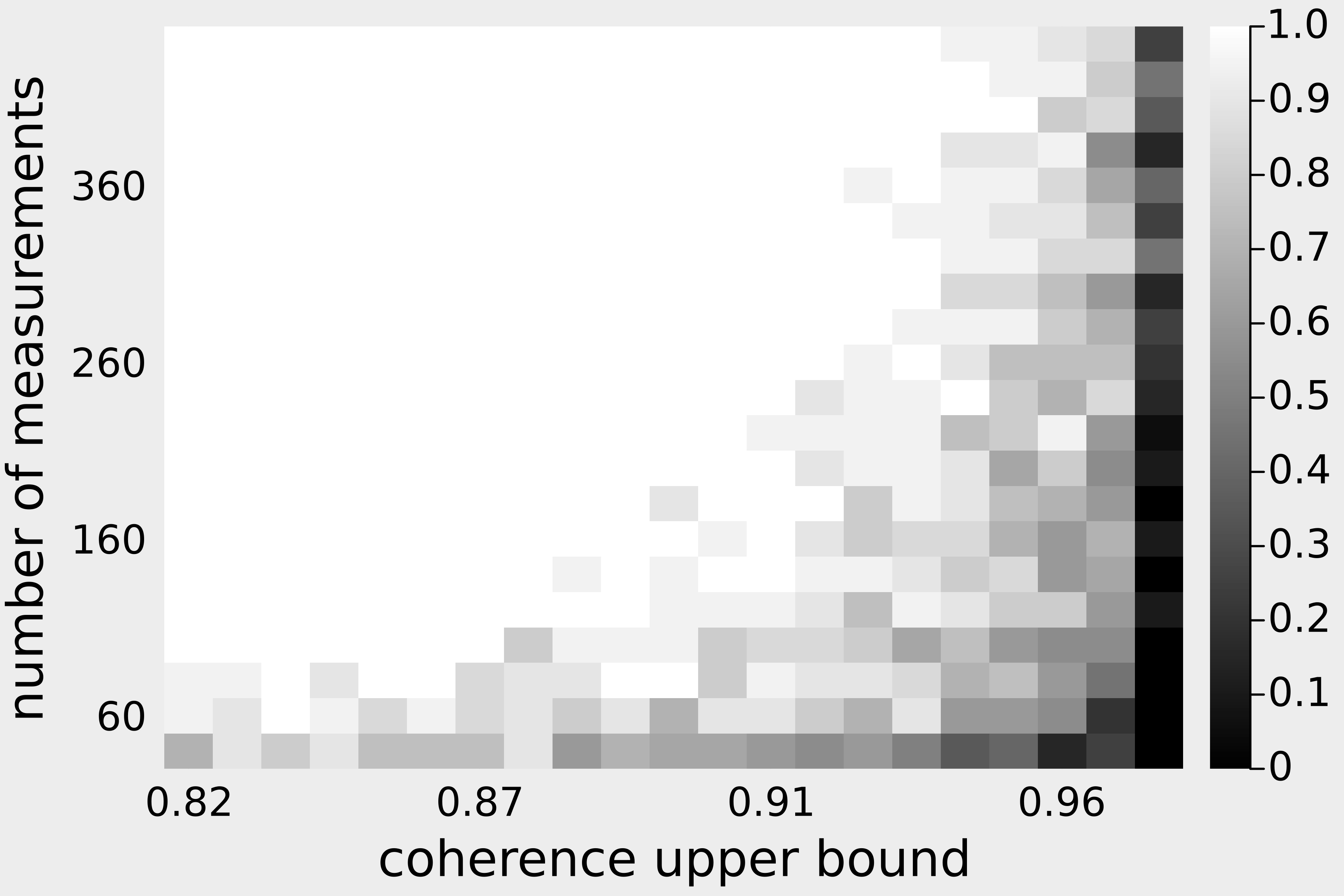
(a) Empirical recovery probability as a function of coherence and $m$. Each block corresponds to the average from 20 independent trials. White corresponds with 20 successful recoveries (rre $\leq 10^{-5}$); black with no successful recoveries.

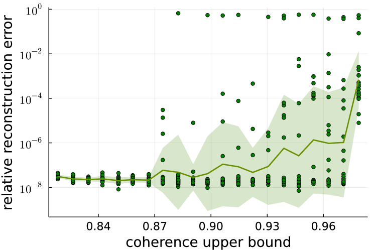
(b) Empirical rre as a function of coherence for $m=100$. Each dot corresponds to one of 20 trials at each coherence level. The solid line shows the empirical geometric mean rre vs. coherence upper bound. The envelope shows $1$ geometric standard deviation.

Figure 1: Dependence of recovery on coherence and number of measurements $m$ for GNNs trained on MNIST.

The results of the first experiment appear in Figure 1. Specifically, 1(a) plots the fraction of successful recoveries from 20 independent trials as a function of the coherence heuristic (2) and number of measurements. White squares correspond to $100\%$ successful recovery (all errors were below $10^{-5}$), while black squares correspond to no successful recoveries (all errors were above $10^{-5}$). In 1(b), we show a slice of the phase plot for $m=100$, plotting rre as a function of the coherence heuristic (2). Each dot corresponds to one of 20 trials at each coherence level. The plot is shown on a $\log$-$y$ scale. The solid line plots the geometric mean of rre as a function of coherence, with an envelope representing $1$ geometric standard deviation (see [51, App. A.1.3] for more information on this visualization strategy). Figure 1 indicates that coherence may be effectively controlled via the heuristic (2), and that coherence is a natural quantity associated with recovery performance. These findings corroborate our theoretical results.

IV-B2 Incoherent networks require fewer measurements

In the second experiment, we provide compelling numerical simulations that support our regularization strategy for lowering coherence of the trained network, resulting in stable recovery of the target signal with much fewer measurements. The results of the second experiment are shown in Figure 2 and Figure 3. In Figure 2, we show the recovered image for three images from the MNIST test set.

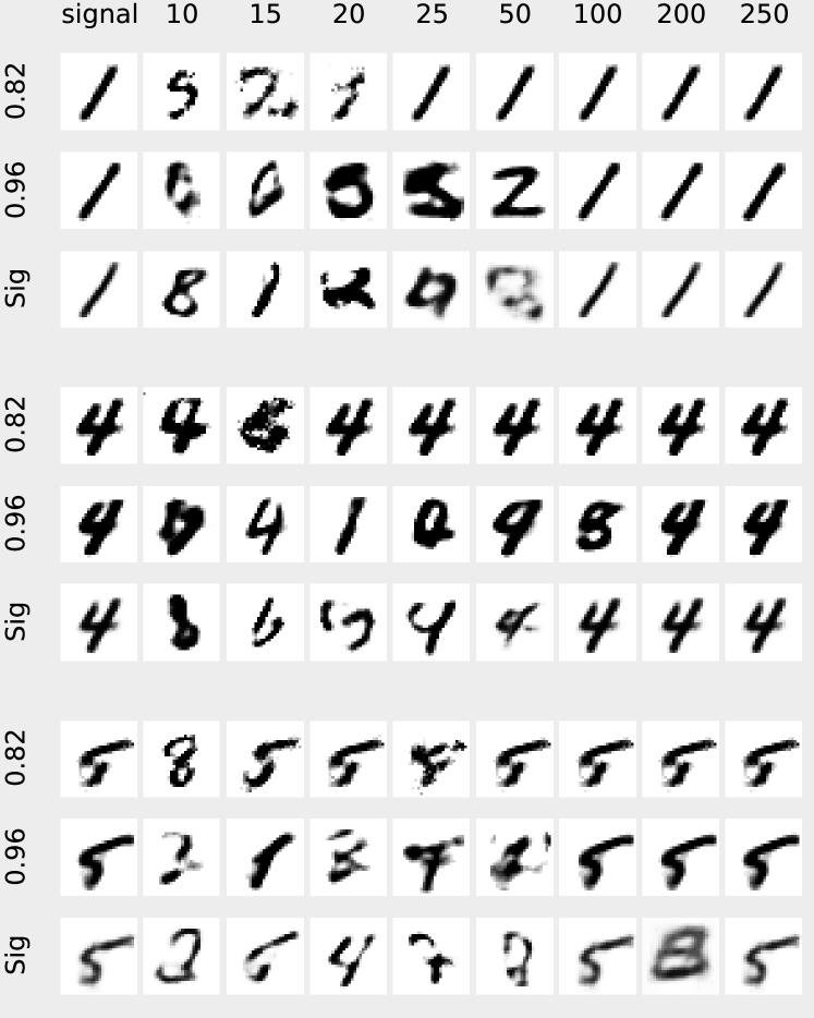
Figure 2: Recovery comparison of MNIST images for various measurement sizes $m$ (denoted by column heading) for a low coherence network, high-coherence network and network with final sigmoid activation. In each block: the top row corresponds to $G^{(3)}$ ($\alpha=0.82$); middle row $G^{(2)}$ ($\alpha=0.96$); bottom row $G^{(1)}$ (labelled Sig). The leftmost column, signal, corresponds to the target image $x_{0}^{(i)}\in\operatorname{\mathcal{R}}(G^{(i)})$.

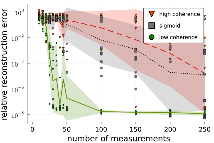
Figure 3: Performance comparison for three GNNs trained on the MNIST dataset — one with low coherence, another with high coherence, and the last with sigmoid activation on the last layer. Plotted against number of measurements $m$ is $\operatorname{rre}$. For each value of $m$, each dot corresponds to one of 10 trials. In each trial, a random image drawn from the MNIST test partition was used as the target signal. Lines depict the empirical geometric mean rre as a function of $m$; shaded regions correspond to $1$ geometric standard deviation. The solid line corresponds to $G^{(3)}$; the dashed line to $G^{(2)}$; the dotted line to $G^{(1)}$.

For each block of $3\times 9$ images, the top row corresponds with the low coherence $G^{(3)}$ ($\alpha=0.82$); the middle row, the high coherence $G^{(2)}$ ($\alpha=0.96$); and the bottom row, $G^{(1)}$, which uses sigmoid activation. The left-most column is the target image belonging to $\operatorname{\mathcal{R}}(G^{(i)})$, labelled signal. All images were clamped to the range $[0,1]$. The figure shows that a GNN with low coherence can effectively recover the target signal with much fewer measurements compared to a network with high coherence, even when that network uses a final sigmoid activation function (which is a realistic choice in practical settings). Remarkably, in some cases we observed that images could be recovered with fewer than $k$ measurements. This highlights the importance of regularizing for networks with low coherence during training. In Figure 3, we further provide empirical evidence of the benefit of low coherence for recovery. For each measurement, we show the results of 10 independent trials for $G^{(1)}$ (squares), $G^{(2)}$ (triangles) and $G^{(3)}$ (circles), respectively. The lines correspond to the empirical geometric mean rre for each network: the dotted line is associated with $G^{(1)}$; the dashed line, the high coherence $G^{(2)}$ ($\alpha=0.96$); and the solid line, the low coherence $G^{(3)}$ ($\alpha=0.82$). The data are plotted on a $\log$-$y$ scale. Each shaded envelope corresponds to $1$ geometric standard deviation about the respective geometric means. This figure empirically supports that high probability successful recovery is achieved with markedly lower sample complexity for the lower coherence network $G^{(3)}$, as compared with either $G^{(2)}$ or $G^{(1)}$. This finding corroborates our theoretical results.

V Proofs

V-A Proofs for Main results

We proceed by proving Theorem II.2, then Theorem II.1. Note that Section II, needed for Theorem II.1, follows immediately from Theorem II.2 using Remark S2.3.

Proof of Theorem II.2.

By construction, $\operatorname{\mathcal{R}}(G)\subseteq\Delta(\operatorname{\mathcal{R}}(G))$; the latter set is a union of linear subspaces (see Definition II.1 and Remark S3.1). By Section S2, $\operatorname{\mathcal{R}}(G)$ is a union of no more than $N$ polyhedral cones of dimension at most $k$, with $N$ satisfying

$$\log N\leq k\sum_{i=1}^{d-1}\log\left(\frac{2ek_{i}}{k}\right)$$

via Remark S2.2. In particular, $\Delta(\operatorname{\mathcal{R}}(G))$ is a collection of at most $N$ subspaces. For any linear subspace $\mathcal{L}\in\Delta(\operatorname{\mathcal{R}}(G))$, observe that $\mathcal{L}$ is $\alpha$-coherent with respect to $\|\cdot\|_{U}$ by assumption. Consequently, by a union bound and application of Section II,

$$\operatorname*{\mathbb{P}}\left\{\sup_{x\in\operatorname{\mathcal{R}}(G)\cap\mathbb{S}^{{n}-1}}\left|\|Ax\|_{2}-1\right|\geq\delta\right\}$$

$$\leq\sum_{\mathcal{L}\in\Delta(\operatorname{\mathcal{R}}(G))}\operatorname*{\mathbb{P}}\left\{\sup_{x\in\mathcal{L}\cap\mathbb{S}^{{n}-1}}\left|\|Ax\|_{2}-1\right|\geq\delta\right\}$$

$$\leq 2Nk\exp\left(-\frac{Cm\delta^{2}}{\alpha^{2}n}\right).$$

The latter quantity is bounded above by $\varepsilon$ if

$$m\gtrsim\frac{\alpha^{2}n}{\delta^{2}}\left(\log N+\log\frac{2k}{\varepsilon}\right),$$

whence, by substituting the bound for $\log N$, it suffices to take

$$m\gtrsim\frac{\alpha^{2}n}{\delta^{2}}\left(k\sum_{i=1}^{d-1}\log\left(\frac{2ek_{i}}{k}\right)+\log\frac{2k}{\varepsilon}\right).$$

∎

Proof of Theorem II.1.

Recall $x^{\perp}:=x_{0}-\operatorname{\Pi}_{\operatorname{\mathcal{R}}(G)}x_{0}$. By triangle inequality and the observation that $\operatorname{\Pi}_{\operatorname{\mathcal{R}}(G)}(x_{0})\in\operatorname{\mathcal{R}}(G)$,

$$\|A\hat{x}-b\|_{2} \leq\min_{x\in\operatorname{\mathcal{R}}(G)}\|Ax-b\|_{2}+\hat{\varepsilon}$$

$$\leq\|A\operatorname{\Pi}_{\operatorname{\mathcal{R}}(G)}(x_{0})-b\|_{2}+\hat{\varepsilon}$$

$$=\|Ax^{\perp}+\eta\|_{2}+\hat{\varepsilon}$$

$$\leq\|Ax^{\perp}\|_{2}+\|\eta\|_{2}+\hat{\varepsilon}.$$

Moreover, with probability at least $1-\varepsilon$ on the realization of $A$, $A$ satisfies a restricted isometry condition on the difference set $\operatorname{\mathcal{R}}(G)-\operatorname{\mathcal{R}}(G)$ by Section II. Therefore, since $\hat{x},\operatorname{\Pi}_{\operatorname{\mathcal{R}}(G)}(x_{0})\in\operatorname{\mathcal{R}}(G)$,

$$\|A\hat{x}-b\|_{2}$$

$$=\left\|A\left(\hat{x}-\operatorname{\Pi}_{\operatorname{\mathcal{R}}(G)}(x_{0})\right)-A\left(x_{0}-\operatorname{\Pi}_{\operatorname{\mathcal{R}}(G)}(x_{0})\right)-\eta\right\|_{2}$$

$$\geq\left\|A\left(\hat{x}-\operatorname{\Pi}_{\operatorname{\mathcal{R}}(G)}(x_{0})\right)\right\|_{2}-\|Ax^{\perp}\|_{2}-\|\eta\|_{2}$$

$$\geq(1-\delta)\left\|\hat{x}-\operatorname{\Pi}_{\operatorname{\mathcal{R}}(G)}(x_{0})\right\|_{2}-\|Ax^{\perp}\|_{2}-\|\eta\|_{2}.$$

Assembling the two inequalities gives

$$\left\|\hat{x}-\operatorname{\Pi}_{\operatorname{\mathcal{R}}(G)}(x_{0})\right\|_{2}\leq\frac{1}{1-\delta}\left[2\|Ax^{\perp}\|_{2}+2\|\eta\|_{2}+\hat{\varepsilon}\right].$$

Finally, apply triangle inequality and choose $\delta=\frac{1}{3}$ to get

$$\|\hat{x}-x_{0}\|_{2} \leq\|x_{0}-\operatorname{\Pi}_{\operatorname{\mathcal{R}}(G)}(x_{0})\|_{2}+\|\hat{x}-\operatorname{\Pi}_{\operatorname{\mathcal{R}}(G)}(x_{0})\|_{2}$$

$$\leq\|x^{\perp}\|_{2}+3\|Ax^{\perp}\|_{2}+3\|\eta\|_{2}+\frac{3}{2}\hat{\varepsilon}.$$

∎

Proof of Section II.

Observe that $I=\sum_{i=1}^{n}U_{i}U_{i}^{*}$ since $U$ is a unitary matrix. Thus, since $\operatorname{\Pi}_{\mathcal{L}}^{2}=\operatorname{\Pi}_{\mathcal{L}}$,

$$\sup_{x\in\mathcal{L}\cap\mathbb{S}^{{n}-1}}\left|\|Ax\|_{2}^{2}-1\right|$$

$$=\sup_{x\in\mathcal{L}\cap\mathbb{S}^{{n}-1}}\left|x^{\top}(A^{*}A-I)x\right|$$

$$=\sup_{x\in\mathcal{L}\cap\mathbb{S}^{{n}-1}}\left|x^{\top}\operatorname{\Pi}_{\mathcal{L}}^{\top}\left(\frac{n}{m}\sum_{i=1}^{n}\theta_{i}U_{i}U_{i}^{*}-\sum_{i=1}^{n}U_{i}U_{i}^{*}\right)\operatorname{\Pi}_{\mathcal{L}}x\right|.$$

Define $\tilde{U}_{i}:=\operatorname{\Pi}_{\mathcal{L}}U_{i}=\operatorname{\Pi}_{\mathcal{L}}^{\top}U_{i}$, using that $\operatorname{\Pi}_{\mathcal{L}}$ is an orthogonal projection, hence symmetric. Then,

$$\sup_{x\in\mathcal{L}\cap\mathbb{S}^{{n}-1}}\left|\|Ax\|_{2}^{2}-1\right|$$

$$=\sup_{x\in\mathcal{L}\cap\mathbb{S}^{{n}-1}}\left|x^{\top}\frac{n}{m}\left(\sum_{i=1}^{n}\left(\theta_{i}-\frac{m}{n}\right)\tilde{U}_{i}\tilde{U}_{i}^{*}\right)x\right|.$$

Since $x$ and $\tilde{U}_{i}$ belong to a $k$-dimensional subspace, there exists a linear isometric embedding $E:\mathbb{R}^{k}\to\mathcal{L}\subseteq{\mathbb{R}^{n}}$ such that $x=E\check{x}$ and $\tilde{U}_{i}=E\check{U}_{i}$ with $\check{x},\check{U}_{i}\in\mathbb{R}^{k}$. Thus,

$$\sup_{x\in\mathcal{L}\cap\mathbb{S}^{{n}-1}}\left|x^{\top}\frac{n}{m}\left(\sum_{i=1}^{n}\left(\theta_{i}-\frac{m}{n}\right)\tilde{U}_{i}\tilde{U}_{i}^{*}\right)x\right|$$

$$=\sup_{x\in\mathbb{S}^{{k}-1}}\left|x^{\top}E^{\top}\frac{n}{m}\left(\sum_{i=1}^{n}\left(\theta_{i}-\frac{m}{n}\right)E\check{U}_{i}\check{U}_{i}^{*}E^{\top}\right)Ex\right|$$

$$=\sup_{x\in\mathbb{S}^{{k}-1}}\left|x^{\top}\frac{n}{m}\left(\sum_{i=1}^{n}\left(\theta_{i}-\frac{m}{n}\right)\check{U}_{i}\check{U}_{i}^{*}\right)x\right|$$

$$=\left\|\frac{n}{m}\sum_{i=1}^{n}\left(\theta_{i}-\frac{m}{n}\right)\check{U}_{i}\check{U}_{i}^{*}\right\|,$$

where, in this case, $\|\cdot\|$ is the operator norm on Hermitian matrices over $\mathbb{R}^{k}$ induced by the Euclidean norm. We will apply the matrix Bernstein inequality (Section S1-A) to achieve concentration of the operator norm of the sum of mean-zero random matrices above. By the $\alpha$-coherence assumption, $\|\check{U}_{i}\|_{2}^{2}=\|\tilde{U}_{i}\|_{2}^{2}=\sup_{x\in\mathcal{L}\cap\mathbb{S}^{{n}-1}}\left|\langle x,U_{i}\rangle\right|^{2}\leq\alpha^{2}$. Consequently, the operator norm of each constituent matrix is bounded almost surely: for each $i\in[n]$,

$$\left\|\frac{n}{m}\check{U}_{i}\check{U}_{i}^{*}\left(\theta_{i}-\frac{m}{n}\right)\right\|\leq\frac{n}{m}\left\|\check{U}_{i}\check{U}_{i}^{*}\right\|=\frac{n}{m}\|\tilde{U}_{i}\|_{2}^{2}\leq\frac{n}{m}\alpha^{2}$$

and the operator norm of the covariance matrix is bounded as

$$\left\|\frac{n^{2}}{m^{2}}\sum_{i=1}^{n}\|\check{U}_{i}\|_{2}^{2}\check{U}_{i}\check{U}_{i}^{*}\operatorname{\mathbb{E}}\left(\theta_{i}-\frac{m}{n}\right)^{2}\right\|$$

$$=\left\|\frac{n^{2}}{m^{2}}\sum_{i=1}^{n}\|\check{U}_{i}\|_{2}^{2}\check{U}_{i}\check{U}_{i}^{*}\frac{m}{n}\left(1-\frac{m}{n}\right)\right\|\leq\alpha^{2}\left(\frac{n}{m}-1\right).$$

Therefore, by Section S1-A it follows that

$$\operatorname*{\mathbb{P}}\left\{\left\|\frac{n}{m}\sum_{i=1}^{n}\check{U}_{i}\check{U}_{i}^{*}\left(\theta_{i}-\frac{m}{n}\right)\right\|\geq\delta\right\}$$

$$\leq 2k\exp\left(-\frac{m\delta^{2}/2}{n\alpha^{2}\left(1-\frac{m}{n}+\frac{\delta}{3}\right)}\right)$$

$$\leq 2k\exp\left(-C\cdot\min\left\{\frac{m\delta^{2}}{n\alpha^{2}(1-m/n)},\frac{m\delta}{n\alpha^{2}}\right\}\right).$$

To complete the proof, we adapt the argument from the proof of [41, Theorem 3.1.1]. Indeed, for $\delta,z\geq 0$ note that $|1-z|>\delta\implies|z^{2}-1|>\max(\delta,\delta^{2})$ yields the implication $\max_{i}|1-z_{i}|>\delta\implies\max_{i}|z_{i}^{2}-1|>\max(\delta,\delta^{2})$. Consequently,

$$\operatorname*{\mathbb{P}}\left\{\sup_{x\in\mathcal{L}\cap\mathbb{S}^{{n}-1}}\left|\|Ax\|_{2}-1\right|\geq\delta\right\}$$

$$\leq\operatorname*{\mathbb{P}}\left\{\sup_{x\in\mathcal{L}\cap\mathbb{S}^{{n}-1}}\left|\|Ax\|_{2}^{2}-1\right|\geq\max(\delta,\delta^{2})\right\}$$

$$\leq 2k\exp\left(-\frac{C\delta^{2}m}{\alpha^{2}n}\right).$$

∎

V-B Proofs for Typical Coherence

The proof of Section III requires the following lemma.

Lemma .

Let $A\in\mathbb{C}^{n\times k}$ be a matrix with $\ell_{2}$-normalized columns and let $A_{i}$ denote the $i$th row of $A$. Then

$$\max_{i\in[n]}\|A_{i}\|_{2}\geq\sqrt{\frac{k}{n}}.$$

Proof of Section V-B.

Computing directly, using that each of the $k$ columns has unit norm,

$$\max_{i\in[n]}\|A_{i}\|_{2}^{2} \geq\operatornamewithlimits{mean}_{i\in[n]}\|A_{i}\|_{2}^{2}=\frac{1}{n}\|A\|_{F}^{2}=\frac{k}{n}.$$

Taking square roots completes the proof. ∎

We now prove the proposition using the lemma.

Proof of Section III.

Take the set $\mathcal{T}$ of all subspaces of dimension $k$ in $\mathbb{C}^{n}$. By rotational invariance of $\mathcal{T}$, it suffices to show the result with respect to $U=I$. Hence, let $\{e_{i}\}_{i\in[n]}$ be the canonical basis. Any fixed $T\in\mathcal{T}$ has coherence

$$\alpha=\sup_{v\in T\cap\mathbb{S}^{{n}-1}}\|v\|_{\infty}.$$

We will show a sharp lower bound on the coherence of all $k$-dimensional subspaces, namely

$$\inf_{T\in\mathcal{T}}\sup_{v\in T\cap\mathbb{S}^{{n}-1}}\|v\|_{\infty}=\sqrt{\frac{k}{n}}.$$

Take the set $\mathcal{A}\subseteq\mathbb{C}^{n\times k}$ of orthonormal matrices. Since $\mathcal{T}=\{\operatorname{\mathcal{R}}(A):A\in\mathcal{A}\}$, it follows that

$$\inf_{T\in\mathcal{T}}\sup_{v\in T\cap\mathbb{S}^{{n}-1}}\|v\|_{\infty} =\inf_{A\in\mathcal{A}}\sup_{\nu\in\mathbb{S}^{k-1}}\|A\nu\|_{\infty}$$

$$=\inf_{A\in\mathcal{A}}\max_{i\in[n]}\sup_{\nu\in\mathbb{S}^{k-1}}|A_{i}\nu|$$

$$=\inf_{A\in\mathcal{A}}\max_{i\in[n]}\|A_{i}\|_{2}.$$

Apply Section V-B to lower bound the latter quantity. As Section V-B applies to any matrix in $\mathcal{A}$,

$$\inf_{A\in\mathcal{A}}\sup_{i\in[n]}\|A_{i}\|_{2}\geq\sqrt{\frac{k}{n}}.$$

We next show that there exists a subspace such that equality holds. Take $F\in\mathbb{C}^{n\times k}$ whose columns are the first $k$ columns of the DFT matrix, as defined in Remark I.1. The columns of $F$ are orthonormal, so $F\in\mathcal{A}$. Furthermore, each row of $F$ has $\ell_{2}$ norm $\sqrt{\frac{k}{n}}$. It follows that

$$\inf_{A\in\mathcal{A}}\max_{i\in[n]}\|A_{i}\|_{2}=\sqrt{\frac{k}{n}}.$$

∎

The proof of Theorem III.1 uses Section S1-C and the following lemma, which bounds the coherence of a random subspace sampled from the Grassmannian. The Grassmanian $\operatorname{\Gamma}_{n,k}$ consists of all $k$-dimensional subspaces of $\mathbb{R}^{n}$ [41, Ch. 5.2.6].

Lemma .

Let $U\in\mathbb{C}^{n\times n}$ be a unitary matrix and denote by $\mathcal{L}\in\operatorname{\Gamma}_{n,k}$ a subspace distributed uniformly at random over $\operatorname{\Gamma}_{n,k}$. With probability at least $1-2\exp(-\gamma^{2})$, $\mathcal{L}$ is $\alpha$-coherent with respect to $\|\cdot\|_{U}$ with

$$\alpha\lesssim\sqrt{\frac{k}{n}}+\sqrt{\frac{\log(n)}{n}}+\frac{\gamma}{\sqrt{n}}.$$

Proof of  Theorem III.1.

Let

$$\tilde{G}(x)=\sigma(W^{(d-1)}\cdots\sigma(W^{(1)}x))$$

so that $G(x)=W^{(d)}\tilde{G}(x)$. Then,

$$\Delta(\operatorname{\mathcal{R}}(G)-\operatorname{\mathcal{R}}(G)) =\Delta\left(W^{(d)}(\operatorname{\mathcal{R}}(\tilde{G})-\operatorname{\mathcal{R}}(\tilde{G}))\right)$$

$$=W^{(d)}\Delta\left(\operatorname{\mathcal{R}}(\tilde{G})-\operatorname{\mathcal{R}}(\tilde{G})\right).$$

By Section S2 and Remark S3.1, $\Delta(\operatorname{\mathcal{R}}(\tilde{G})-\operatorname{\mathcal{R}}(\tilde{G}))$ is the union of $M$ at-most $2k$-dimensional linear subspaces with

$$\log M\leq 2k\sum_{i=1}^{d-1}\log\left(\frac{2ek_{i}}{k}\right).$$

Each subspace $\mathcal{L}$ is uniformly distributed on $\operatorname{\Gamma}_{n,\dim\mathcal{L}}$, where $\dim\mathcal{L}\leq 2k$, because the final weight matrix has iid Gaussian entries independent of the other weight matrices (e.g., see [41, Ch. 3.3.2]). Enumerate the subspaces from $1$ to $M$ (independently of $W^{(d)}$). Then, applying Section V-B, we see that the coherence of subspace $i$ is a random variable $\alpha_{i}$ such that

$$\alpha_{i}\lesssim\sqrt{\frac{k}{n}}+\sqrt{\frac{\log(n)}{n}}+\frac{\gamma}{\sqrt{n}}$$

with probability at least $1-2\exp(-\gamma^{2})$.

Let $\alpha$ be the coherence of $\Delta(\operatorname{\mathcal{R}}(G)-\operatorname{\mathcal{R}}(G))$ and observe that $\alpha\leq\max_{i\in[M]}\alpha_{i}$. Applying Section S1-C,

$$\alpha\leq\max_{i\in[M]}\alpha_{i}\lesssim\sqrt{\frac{k}{n}}+\sqrt{\frac{\log(n)}{n}}+\sqrt{\frac{\log M}{n}}+\frac{\gamma}{\sqrt{n}}$$

with probability at least $1-2\exp(-\gamma^{2})$. ∎

We next prove Section V-B.

Proof of  Section V-B.

Let $A\in\mathbb{R}^{n\times k}$ with $A_{ij}\overset{\text{iid}}{\sim}\mathcal{N}(0,1)$. Then, $\mathcal{L}:=\operatorname{\mathcal{R}}(A)$ is a random subspace uniformly distributed over $\operatorname{\Gamma}_{n,k}$. By rotation invariance of the Grassmannian, it suffices to show the result for $U=I$. Let $\{e_{i}\}_{i\in[n]}$ denote the canonical basis. Define

$$\alpha:=\sup_{v\in\mathcal{L}\cap\mathbb{S}^{{n}-1}}\max_{i\in[n]}\left|\langle e_{i},v\rangle\right|,$$

and note that $\mathcal{L}$ is $\alpha$-coherent with respect to $\|\cdot\|_{I}=\|\cdot\|_{\infty}$. For each $i\in[n]$, we next analyze

$$\alpha_{i}:=\sup_{v\in\mathcal{L}\cap\mathbb{S}^{{n}-1}}|\langle e_{i},v\rangle|=\sup_{y\in\mathbb{S}^{k-1}}\left|\frac{A_{i}y}{\|Ay\|_{2}}\right|.$$ (4)

We will show, with probability at least $1-4\exp(-s^{2})$,

$$\alpha_{i}\lesssim\sqrt{\frac{k}{n}}+\frac{s}{\sqrt{n}}.$$

To see why this result should hold, we focus our attention on the right hand side of (4). The denominator concentrates around $\sqrt{n}$ and the numerator is bounded by $\|A_{i}\|_{2}$, which concentrates around $\sqrt{k}$ with subgaussian tails.

We first obtain a lower bound on the smallest singular value of $A$ via [41, Theorem 4.6.1], which guarantees with probability at least $1-2\exp(-t^{2})$ that

$$\inf_{y\in\mathbb{S}^{k-1}}\|Ay\|_{2}\geq\sqrt{n}-C\sqrt{k}-Ct.$$

By fixing $t=\frac{\sqrt{n}}{2C}$ we define the event

$$B:=\left\{\inf_{y\in\mathbb{S}^{k-1}}\|Ay\|_{2}\leq\frac{\sqrt{n}}{2}-C\sqrt{k}\right\}$$

satisfying $\operatorname*{\mathbb{P}}\left\{B\right\}\leq 2\exp(-cn)$. We first limit $s$ so that $\sqrt{k}+s\leq\frac{\sqrt{n}}{2}-C\sqrt{k}$, which implies that $s<C\sqrt{n}$. Then

$$\operatorname*{\mathbb{P}}\left\{\sup_{y\in\mathbb{S}^{k-1}}\frac{A_{i}y}{\|Ay\|_{2}}>\frac{\sqrt{k}+s}{\frac{\sqrt{n}}{2}-C\sqrt{k}}\right\}$$

$$=\operatorname*{\mathbb{P}}\left\{\sup_{y\in\mathbb{S}^{k-1}}\frac{A_{i}y}{\|Ay\|_{2}}>\frac{\sqrt{k}+s}{\frac{\sqrt{n}}{2}-C\sqrt{k}}\Big{|}B\right\}\operatorname*{\mathbb{P}}\left\{B\right\}$$

$$+\operatorname*{\mathbb{P}}\left\{\sup_{y\in\mathbb{S}^{k-1}}\frac{A_{i}y}{\|Ay\|_{2}}>\frac{\sqrt{k}+s}{\frac{\sqrt{n}}{2}-C\sqrt{k}}\Big{|}B^{c}\right\}\operatorname*{\mathbb{P}}\left\{B^{c}\right\}$$

$$\leq\operatorname*{\mathbb{P}}\{B\}+\operatorname*{\mathbb{P}}\left\{\sup_{y\in\mathbb{S}^{k-1}}A_{i}y>\sqrt{k}+s\right\}$$

$$\leq 2\exp(-cn)+\operatorname*{\mathbb{P}}\left\{\|A_{i}\|_{2}>\sqrt{k}+s\right\}$$

$$\leq 2\exp(-cn)+2\exp(-cs^{2}).$$

Above, we used the concentration of the norm of Gaussian vectors [41, Theorem 3.1.1]. Since $s\leq C\sqrt{n}$, $\exp(-cn)\leq\exp(-cs^{2})$. From this we find the desired subgaussian tail bound:

$$\operatorname*{\mathbb{P}}\left\{\sup_{y\in\mathbb{S}^{k-1}}\frac{A_{i}y}{\|Ay\|_{2}}>\frac{\sqrt{k}+s}{\frac{\sqrt{n}}{2}-C\sqrt{k}}\right\}\leq 4\exp(-cs^{2}).$$

The remaining values of $s$ satisfy $\sqrt{k}+s>\frac{\sqrt{n}}{2}-C\sqrt{k}$. Therefore, since $\sup_{y\in\mathbb{S}^{k-1}}\frac{A_{i}y}{\|Ay\|_{2}}\leq 1$,

$$\operatorname*{\mathbb{P}}\left\{\sup_{y\in\mathbb{S}^{k-1}}\frac{A_{i}y}{\|Ay\|_{2}}>\frac{\sqrt{k}+s}{\frac{\sqrt{n}}{2}-C\sqrt{k}}\right\}=0\leq 4\exp(-cs^{2}).$$

Therefore, the subgaussian bound applies for all values of $s$.

We now scale $s$ by an absolute constant with $\gamma=cs$. Then

$$\alpha_{i}=\sup_{y\in\mathbb{S}^{k-1}}\left|\frac{A_{i}y}{\|Ay\|_{2}}\right|>\frac{\sqrt{k}+s}{\frac{\sqrt{n}}{2}-C\sqrt{k}}\gtrsim\sqrt{\frac{k}{n}}+\frac{\gamma}{\sqrt{n}}$$

with probability less than $2\exp(-\gamma^{2})$. Changing the constant from 4 to 2 in the probability bound is achieved by suitable choice of $c$. Remembering that $\alpha$ is the coherence with the canonical basis, we apply Section S1-C to find,

$$\alpha=\max_{i\in[n]}\alpha_{i}\lesssim\sqrt{\frac{k}{n}}+\sqrt{\frac{\log n}{n}}+\frac{\gamma}{\sqrt{n}}$$

with probability at least $1-2\exp(-\gamma^{2})$. ∎

VI Conclusion

In this work, we have proved a restricted isometry property for a subsampled isometry with GNN structural proxy, Theorem II.2. We used this to prove sample complexity and recovery bounds, Theorem II.1. The recovery bound stated in Theorem II.1 is uniform over ground truth signals, and permits a more finely tuned nonuniform control as discussed in Remark II.2. To our knowledge, this provides the first theory for generative compressed sensing with subsampled isometries and non-random weights.

Our results rely on the notion of $\alpha$-coherence with respect to the measurement norm, introduced in Definition I.4 and Definition I.3, respectively. Closely related to the notion of incoherent bases [7, p. 373] and the $X$-norm of [13], we argue that $\alpha$-coherence is a natural quantity to measure the interplay between a GNN and the measurement operator. Indeed, in Section IV we propose a regularization strategy for promoting favourable coherence of GNNs during training, and connect this strategy with favourable recovery efficacy. Specifically, we show that our regularization strategy yields low coherence GNNs with improved sample complexity for recovery (Figure 3). Moreover, our numerics support that low coherence GNNs achieve better sample complexity than high coherence GNNs (Figure 1).

We suspect the $\Omega(k^{2}d^{2})$ dependence in the sample complexity of our analysis is sub-optimal, and a consequence of our coherence-based approach. Ignoring logarithmic factors, it is an open question to prove recovery guarantees with $\Omega(kd)$ Fourier measurements and non-random weights, which would match the number of (sub-)Gaussian measurements needed [1] and would also match the known worst-case lower bound [52]. In addition, it is an open problem to improve the regularization strategy for lowering coherence, possibly including middle layers. Finally, it is open to determine a notion of coherence for networks that have a final nonlinear activation function, and to characterize how this impacts recovery efficacy for such networks.

Supplementary material

This supplementary material contains auxiliary results from high-dimensional probability (Section S1); a characterization of the range of a generative network and an elaboration on properties of the operator $\Delta$ (Section S2 and Section S3 respectively); a discussion concerning control of the approximation error (Section S4) as it pertains to Remark II.2; and an epilogue (Section S5), whose purpose is to clarify the role of our mathematical argument in its determination of the sample complexity.

S1 Results from high-dimensional probability

S1-A Matrix Bernstein inequality

For this result, see [53, Theorem 6.1].

Lemma (Matrix Bernstein inequality).

Let $X_{1},\ldots,X_{N}\in\mathbb{C}^{n\times n}$ be independent, mean-zero, self-adjoint random matrices, such that $\|X_{i}\|\leq K$ almost surely for all $i$. Then, for every $\gamma\geq 0$ we have

$$\operatorname*{\mathbb{P}}\left\{\left\|\sum_{i=1}^{N}X_{i}\right\|\geq\gamma\right\} \leq 2n\exp\left(-\frac{\gamma^{2}/2}{\tau^{2}+K\gamma/3}\right)$$

$$\leq 2n\exp\left(-c\cdot\min\left(\frac{\gamma^{2}}{\tau^{2}},\frac{\gamma}{K}\right)\right).$$

Here, $\tau^{2}:=\left\|\sum_{i=1}^{N}\operatorname{\mathbb{E}}X_{i}^{2}\right\|$.

S1-B Cramér-Chernoff bound

For a reference to this material, see [54, Ch. 2.2]. Let $Z$ be a real-valued random variable. Then,

$$\operatorname*{\mathbb{P}}\left\{Z\geq t\right\} \leq\exp(-\psi_{Z}^{*}(t)), \psi_{Z}^{*}(t) :=\sup_{\lambda\geq 0}\lambda t-\psi_{Z}(\lambda).$$

The latter quantity, $\psi_{Z}^{*}(t)$, is the Cramér transform of $Z$, with

$$\psi_{Z}(\lambda):=\log\operatorname{\mathbb{E}}\exp(\lambda Z),\quad\lambda\geq 0$$

being the logarithm of the moment generating function of $Z$. When $Z$ is centered, $\psi_{Z}$ is continuously differentiable on an interval of the form $[0,b)$ and $\psi_{Z}(0)=\psi^{\prime}_{Z}(0)=0$. Thus,

$$\psi^{*}_{Z}(t)=\lambda_{t}t-\psi_{Z}(\lambda_{t}),$$

where $\lambda_{t}$ is such that $\psi^{\prime}_{Z}(\lambda_{t})=t$.

For a centered binomial random variable $Z:=Y-np$ where $Y\sim\mathrm{Binom}(n,p)$, the Cramér transform of $Z$ is given by

$$\psi_{Z}^{*}(t) :=nh_{p}\left(\frac{t}{n}+p\right),\quad\forall 0<t<n(1-p),$$

where

$$h_{p}(a):=(1-a)\log\frac{1-a}{1-p}+a\log\frac{a}{p}$$

is the Kullback-Leibler divergence $\operatorname{D_{\mathrm{KL}}}(P_{a}\;\|\;P_{p})$ between Bernoulli distributions with parameters $a$ and $p$. One may thus establish [54, Ch. 2.2] the following concentration inequality for $Y$ when $0<t<\frac{n}{m}$:

$$\operatorname*{\mathbb{P}}\left\{Y\geq tm\right\}=\operatorname*{\mathbb{P}}\left\{Z\geq(t-1)m\right\}\leq\exp(-nh_{p}(tp)).$$

S1-C Auxiliary union bound

Lemma .

Let $f:\mathbb{R}\to\mathbb{R}$ be an increasing function. Let $\{X_{i}\}_{i\in[n]}$ be a collection of random variables such that for each $i\in[n]$ and for any $\gamma>0$,

$$X_{i}\leq f(\gamma)$$

with probability at least $1-2\exp(-\gamma^{2})$. Then, for all $\gamma>0$,

$$\max_{i\in[n]}X_{i}\leq f\left(c\left(\gamma+\sqrt{\log n}\right)\right)$$

with probability at least $1-2\exp(-\gamma^{2})$.

Proof of Section S1-C.

By assumption,

$$\operatorname*{\mathbb{P}}\left\{\max_{i\leq[n]}X_{i}>f(\gamma)\right\} =\operatorname*{\mathbb{P}}\left\{\bigcup_{i\in[n]}\{X_{i}>f(\gamma)\}\right\}$$

$$\leq n2\exp(-\gamma^{2})$$

$$=2\exp(-\gamma^{2}+\log n).$$

Let $t:=\sqrt{\gamma^{2}-\log n}$. We substitute $\gamma^{2}\to t^{2}+\log n$ in the right hand side of the equation above which yields

$$\operatorname*{\mathbb{P}}\left\{\max_{i\leq[n]}X_{i}>f(\gamma)\right\}\leq 2\exp(-t^{2}).$$

To substitute the remaining $\gamma$ on the left hand side, first notice

$$\gamma \leq 2\max\left(t,\sqrt{\log n}\right)\leq 2\left(t+\sqrt{\log n}\right).$$

Consequently, $f(\gamma)\leq f\left(2\left(t+\sqrt{\log n}\right)\right)$ and

$$\operatorname*{\mathbb{P}}\left\{\max_{i\in[n]}X_{i}>f\left(2\left(t+\sqrt{\log n}\right)\right)\right\} \leq\operatorname*{\mathbb{P}}\left\{\max_{i\in[n]}X_{i}>f(\gamma)\right\}$$

$$\leq 2\exp(-t^{2})$$

Re-labelling $t\to\gamma$ yields the result. ∎

S2 Characterizing $\operatorname{\mathcal{R}}(G)$

For completeness, we include a characterization of the geometry of the range of generative neural networks with ReLU activation. This material is not novel; for instance, see [42]. It requires the notion of a low-dimensional cone.

Definition S2.1.

A convex set $\mathcal{C}\subseteq\mathbb{R}^{n}$ is at-most $k$-dimensional for some $k\in[n]$ if there exists a linear subspace $E\subseteq\mathbb{R}^{n}$ with $\dim(E)\leq k$ and $\mathcal{C}\subseteq E$.

Remark S2.1.

A cone $\mathcal{C}\subseteq\mathbb{R}^{n}$ is at-most $k$-dimensional if its linear hull, $\operatorname{\mathrm{span}}(\mathcal{C})$, is no greater than $k$-dimensional. ∎

A key idea in our recovery guarantees will be to cover $\operatorname{\mathcal{R}}(G)$ using at-most $k$-dimensional cones. To this end, it will be important to bound the number $N$ of at-most $k$-dimensional cones in the covering set. This comes down to quantifying the number of different ways that ReLU can act on a given subspace, which reduces to counting the number of orthants that subspace intersects. The following result may be found in [55, App. A Lemma 1].

Lemma (orthant-crossings).

Let $S\subseteq\mathbb{R}^{n}$ be a $k$-dimensional subspace. Then $S$ intersects at most $I(n,k)$ different orthants where

$$I(n,k)\leq 2^{k}\binom{n}{k}\leq 2^{k}\left(\frac{en}{k}\right)^{k}.$$ (5)

Note that previous work [56, 57] has established the bound

$$I(n,k)\leq 2\sum_{\ell=0}^{k-1}\binom{n-1}{\ell},$$

which is tight [56]. Accordingly, the extent of non-tightness of the bound (5) may be evaluated directly for specific choices of $n$ and $k$. The upper bound on $N$ is an immediate consequence. We also require the notion of a polyhedral cone, used in Section S2 below. Note that a version of the lemma may be found in [42].

Definition S2.2 (Polyhedral cone).

A cone $\mathcal{C}\subseteq\mathbb{R}^{n}$ is called polyhedral if it is the conic combination of finitely many vectors. Equivalently, $\mathcal{C}$ is polyhedral if it is the intersection of a finite number of half-spaces that have the origin on their boundary.

Lemma .

Let $G$ be a $(k,d,n)$-generative network with layer widths $k=k_{0}\leq k_{1},\ldots,k_{d}$ where $k_{d}=n$. Then $\operatorname{\mathcal{R}}(G)$ is a union of no more than $N$ at-most $k$-dimensional polyhedral cones where

$$N :=\prod_{\ell=1}^{d-1}I(k_{\ell},k)\leq\left(\frac{2e\bar{k}}{k}\right)^{k(d-1)},$$

$$\bar{k} :=\left(\prod_{\ell=1}^{d-1}k_{\ell}\right)^{1/(d-1)}.$$

Proof of Section S2.

The proof is similar to the one given in [42], repeated here for completeness.

First, if $\mathcal{C}\subseteq\mathbb{R}^{\tilde{n}}$ is a polyhedral cone of dimension $k\leq\tilde{n}$ and $L:\mathbb{R}^{\tilde{n}}\to\mathbb{R}^{n^{\prime}}$ is a linear map with $n^{\prime}\in\mathbb{N}$ then $L\mathcal{C}$ is a polyhedral cone with dimension at most $\min\{k,n^{\prime}\}$. Likewise, the intersection of a collection of polyhedral cones is a polyhedral cone. Now, if $(Q_{i})_{i\in[2^{\tilde{n}}]}$ are the orthants of $\mathbb{R}^{\tilde{n}}$ with $Q_{1}$ being the nonnegative orthant, observe that $\operatorname{\Pi}_{Q_{1}}$ is linear on each orthant $Q_{i}$, $i\in[2^{\tilde{n}}]$. Consequently,

$$\sigma(\mathcal{C})=\bigcup\limits_{i=1}^{2^{\tilde{n}}}\operatorname{\Pi}_{Q_{1}}\left(\mathcal{C}\cap Q_{i}\right)$$

is a union of polyhedral cones. Since the domain $\mathbb{R}^{k}$ of $G$ is a polyhedral cone, it follows that $\sigma\left(W^{(1)}\mathbb{R}^{k}\right)$ is a union of polyhedral cones, and continuing by induction, $\operatorname{\mathcal{R}}(G)$ is a union of polyhedral cones. By the rank-nullity theorem each component cone has dimension at most $k$.

We next argue for the bound $N$ on the number of cones comprising the range. Consider that the final mapping $W^{(d)}$ cannot increase the number of cones. Thus, it suffices to consider the map $\sigma(W^{(d-1)}\cdots\sigma(W^{(1)}u))$. We need only count the number of new intersected subspaces that could be generated from each ReLU operation. As there are $d-1$ in total, we obtain

$$\prod_{\ell=1}^{d-1}I(k_{\ell},k)\leq 2^{(d-1)k}\prod_{\ell=1}^{d-1}\left(\frac{ek_{\ell}}{k}\right)^{k}=\left(\frac{2e\bar{k}}{k}\right)^{k(d-1)},$$

where $\bar{k}$ is the geometric mean $\bar{k}:=\left(\prod_{\ell=1}^{d-1}k_{\ell}\right)^{1/(d-1)}$.∎

Remark S2.2.

A simple calculation shows that

$$\log N\leq k\sum_{i=1}^{d-1}\log\left(\frac{2ek_{i}}{k}\right).$$

∎

Remark S2.3.

If $G$ is a $d$ layer neural network with ReLU activation then $G(x)-G(y)$ can be written as $\bar{G}(x,y):=G(x)-G(y)$ where $\bar{G}:\mathbb{R}^{2k}\to\mathbb{R}^{n}$ is a $d$-layer neural network whose $i$th weight matrix is

$$\left[\begin{array}[]{ll}W^{(i)}&\mathbf{0}_{k_{i}\times k_{i-1}}\\ \mathbf{0}_{k_{i}\times k_{i-1}}&W^{(i)}\end{array}\right]$$

for $i=1,\ldots,d-1$ where $\mathbf{0}_{m,n}$ is the $m\times n$ zero matrix. The $d$th weight matrix of $\bar{G}$ is $\left[\begin{array}[]{rr}W^{(d)}&-W^{(d)}\end{array}\right]$. In particular, the layer widths of $\bar{G}$ are $2k_{0}=2k,2k_{1},\ldots,2k_{d-1},k_{d}=n$, so applying Section S2 to $\bar{G}$ gives

$$N(\bar{G}) \leq\left(\frac{2e\bar{k}}{k}\right)^{2k(d-1)}, \log N(\bar{G}) \leq 2k\sum_{i=1}^{d-1}\log\left(\frac{2ek_{i}}{k}\right),$$

where $\bar{k}$ is the geometric mean of the layer widths of the original network $G$. ∎

Remark S2.4.

We argue that Theorem III.1 extends to GNNs with biases. That the result holds for GNNs with arbitrary fixed biases in all but the last layer follows from the representation of a biased GNN with augmented matrices, see Remark I.2. Allowing for an arbitrary fixed (or random) bias in the last layer then follows, because $\operatorname{\mathcal{R}}(G)-\operatorname{\mathcal{R}}(G)$ is invariant to changes in the bias of the last layer, since it is affine. ∎

S3 Convex cones and the operator $\Delta$

For the following proposition, see [58, Proposition 6.4].

Proposition (Cone difference is subspace).

Let $\mathcal{K}\subseteq\mathbb{R}^{n}$ be a convex cone. Then $\mathcal{K}-\mathcal{K}=\operatorname{\mathrm{span}}\mathcal{K}$.

Remark S3.1.

Below we list several properties about $\Delta$. Let $\mathcal{C}=\bigcup\limits_{i=1}^{N}\mathcal{C}_{i}$ be the union of $N\in\mathbb{N}$ convex cones $\mathcal{C}_{i}$.

1. The latter equality in Definition II.1 follows from Section S3.

2. The set $\Delta(\mathcal{C})$ is uniquely defined. In particular, it is independent of the (finite) decomposition of $\mathcal{C}$ into convex cones.

3. If $\max_{i\in[N]}\dim\mathcal{C}_{i}\leq k$, then $\Delta(\mathcal{C})$ is a union of no more than $N$ at-most $k$-dimensional linear subspaces.

4. The set $\Delta(\mathcal{C})$ satisfies $\mathcal{C}\subseteq\Delta(\mathcal{C})\subseteq\mathcal{C}-\mathcal{C}$.

5. There are choices of $\mathcal{C}$ for which $\mathcal{C}\subsetneq\Delta(\mathcal{C})$ (for instance, refer to the example at the end of this section).

∎

Proof of uniqueness of $\Delta(\mathcal{C})$.

We begin with the following lemma.

Lemma .

Let $N$, $M$ be positive integers, and let $\mathcal{C}_{1},\mathcal{C}_{2},\ldots,\mathcal{C}_{N}$ be convex cones in $\mathbb{R}^{M}$ such that their union $\mathcal{C}$ is also convex. Then, there exists $i\in[N]$ such that $\operatorname{\mathrm{span}}(\mathcal{C})=\operatorname{\mathrm{span}}(\mathcal{C}_{i})$.

Proof of Section S3.

First, assume $\operatorname{\mathrm{span}}(\mathcal{C})=\mathbb{R}^{M}$. Let $\mu$ be the Gaussian measure, so that for a (measurable) set $\mathcal{A}\subseteq\mathbb{R}^{M}$ $\mu(\mathcal{A})=\operatorname*{\mathbb{P}}\{z\in\mathcal{A}\}$, where $z\subset\mathbb{R}^{M}$ has independent standard normal entries. One can show that for any convex cone $\mathcal{B}$, $\mu(\mathcal{B})>0$ if and only if $\operatorname{\mathrm{span}}(\mathcal{B})=\mathbb{R}^{M}$. Then, since $\mathcal{C}$ is convex,

$$0<\mu(\mathcal{C})=\mu\left(\bigcup_{i=1}^{N}\mathcal{C}_{i}\right)\leq\sum_{i=1}^{N}\mu(\mathcal{C}_{i}).$$

Thus, there exists $i\in[N]$ such that $\mu(\mathcal{C}_{i})>0$, whence $\operatorname{\mathrm{span}}(\mathcal{C}_{i})=\mathbb{R}^{M}$. This proves the lemma when $\operatorname{\mathrm{span}}(\mathcal{C})=\mathbb{R}^{M}$.

For the general case, where $\operatorname{\mathrm{span}}(\mathcal{C})=\mathcal{S}$ for some subspace $\mathcal{S}$, replace the Gaussian measure on $\mathbb{R}^{M}$ by the Gaussian measure restricted to that subspace, $\mu_{\mathcal{S}}$, the unique measure satisfying $\mu_{\mathcal{S}}(\mathcal{A})=P(\Pi_{\mathcal{S}}(z)\in\mathcal{A})$. As above, for any convex cone $\mathcal{B}$, clearly $\mu_{\mathcal{S}}(\mathcal{B})>0$ if and only if $\operatorname{\mathrm{span}}(\mathcal{B})=\mathcal{S}$ and the proof proceeds as above. ∎

We now proceed with the proof of uniqueness. Given two collections of convex cones $\mathcal{F}=\{\mathcal{F}_{i}\}_{i\in[N]},\mathcal{D}=\{\mathcal{D}_{i}\}_{i\in[N]}$ such that $\mathcal{C}=\bigcup_{i\in[N]}\mathcal{F}_{i}=\bigcup_{i\in[N]}\mathcal{D}_{i}$, let $\Delta_{\mathcal{F}}(C):=\bigcup_{i\in[N]}\operatorname{\mathrm{span}}(\mathcal{F}_{i})$ and define $\Delta_{\mathcal{D}}(C)$ similarly. It is sufficient to show that $\Delta_{\mathcal{F}}(\mathcal{C})=\Delta_{\mathcal{D}}(\mathcal{C})$. Note that, without loss of generality, we assume that $\mathcal{F}$ and $\mathcal{D}$ have the same number of elements since we can take some cones as the empty set.

Fix $i\in[N]$. Note for all $j\in[N],\ \mathcal{F}_{i}\cap\mathcal{D}_{j}$ is a convex cone. Then, we have

$$\mathcal{F}_{i}=\mathcal{F}_{i}\cap\mathcal{C}=\mathcal{F}_{i}\cap\bigcup_{j\in[N]}\mathcal{D}_{j}=\bigcup_{j\in[N]}(\mathcal{F}_{i}\cap\mathcal{D}_{j}).$$

It then follows from Section S3, that there is a $j^{*}$ such that $\operatorname{\mathrm{span}}(\mathcal{F}_{i})=\operatorname{\mathrm{span}}(\mathcal{F}_{i}\cap\mathcal{D}_{j^{*}})$. Further,

$$\operatorname{\mathrm{span}}(\mathcal{F}_{i}\cap\mathcal{D}_{j^{*}})\subseteq\operatorname{\mathrm{span}}(\mathcal{D}_{j^{*}})\subseteq\Delta(\mathcal{D}).$$

Since this is true for every $i$, $\Delta_{\mathcal{F}}(\mathcal{C})\subseteq\Delta_{\mathcal{D}}(\mathcal{C})$. By symmetry, $\Delta_{\mathcal{D}}(\mathcal{C})\subseteq\Delta_{\mathcal{F}}(\mathcal{C})$, so $\Delta_{\mathcal{D}}(\mathcal{C})=\Delta_{\mathcal{F}}(\mathcal{C})$. ∎

We conclude this section by briefly illuminating the effect of the piecewise linear expansion $\Delta$ using a simple example.

Example.

Define the $(3,2,3)$-generative network:

$$G(z):=\sigma\left(W^{(1)}z\right),\qquad W^{(1)}:=\left[\begin{array}[]{rrr}1&0&0\\ -1&0&0\\ 0&0&0\end{array}\right].$$

Note the second weight matrix for $G$ is the identity matrix. Observe that $\operatorname{\mathcal{R}}(W^{(1)})=\{(x,-x,0):x\in\mathbb{R}\}$, so that

$$\operatorname{\mathcal{R}}(G)=\{\gamma e_{1}:\gamma\geq 0\}\cup\{\gamma e_{2}:\gamma\geq 0\}.$$

Consequently, it is straightforward to show that

$$\Delta(\operatorname{\mathcal{R}}(G)) =\operatorname{\mathrm{span}}\{e_{1}\}\cup\operatorname{\mathrm{span}}\{e_{2}\}$$

$$\operatorname{\mathcal{R}}(G)-\operatorname{\mathcal{R}}(G) =\{(x,y,0):xy\leq 0\}$$

$$\Delta(\operatorname{\mathcal{R}}(G)-\operatorname{\mathcal{R}}(G)) =\operatorname{\mathrm{span}}\{e_{1},e_{2}\}.$$

These sets clearly satisfy the inclusion chain $\operatorname{\mathcal{R}}(G)\subset\Delta(\operatorname{\mathcal{R}}(G))\subset\operatorname{\mathcal{R}}(G)-\operatorname{\mathcal{R}}(G)\subset\Delta(\operatorname{\mathcal{R}}(G)-\operatorname{\mathcal{R}}(G))$. Moreover, note that $\Delta(\operatorname{\mathcal{R}}(G))$ is a particular subset of $1$-sparse vectors in $\mathbb{R}^{3}$ while $\Delta(\operatorname{\mathcal{R}}(G)-\operatorname{\mathcal{R}}(G))$ is a particular subset of $2$-sparse vectors in $\mathbb{R}^{3}$. ∎

S4 Controlling approximation error

Suppose that $A\in\mathbb{C}^{\tilde{m}\times n}$ is an $(m,\theta,U)$-subsampled isometry with associated unitary matrix $U\in\mathbb{C}^{n\times n}$. Recall that $U^{*}U=I$ where $I$ is the identity matrix, and that $\theta_{i}\overset{\text{iid}}{\sim}\mathrm{Ber}\left(\frac{m}{n}\right)$. Let $x\in\mathbb{C}^{n}$ be a fixed vector such that $\|x\|_{2}=1$. We would like to estimate the tail

$$\operatorname*{\mathbb{P}}\left\{\|Ax\|_{2}^{2}\geq t\right\}$$

for $t\geq 1$, so as to imply a high probability bound of the form $\|Ax\|_{2}^{2}\leq t\|x\|_{2}^{2}$ for any fixed $x\in\mathbb{C}^{n}$. For technical reasons yet to be clarified, we also assume $t<n/m$.

S4-A Reformulation

Observe that $A^{*}A=\frac{n}{m}U^{*}\operatorname{\mathrm{diag}}(\theta)U$, implying

$$\|Ax\|_{2}^{2}=x^{*}A^{*}Ax=\frac{n}{m}x^{*}U\operatorname{\mathrm{diag}}(\theta)Ux=\frac{n}{m}\sum_{i=1}^{n}\theta_{i}|z_{i}|^{2},$$

where $z:=Ux$ and $\|z\|_{2}=\|Ux\|_{2}=1$. Hence, the problem can be recast as bounding the following tail:

$$\operatorname*{\mathbb{P}}\left\{\frac{n}{m}\sum_{i=1}^{n}\theta_{i}|z_{i}|^{2}\geq t\right\},$$

for $t>0$ and where $z\in\mathbb{C}^{n}$ is a fixed vector with $\|z\|_{2}=1$.

S4-B Special cases

S4-B1 Spike

Assume that $z:=e_{1}$ is the first standard basis vector. Then

$$\operatorname*{\mathbb{P}}\left\{\frac{n}{m}\sum_{i=1}^{n}\theta_{i}|z_{i}|^{2}\geq t\right\}=\operatorname*{\mathbb{P}}\left\{\theta_{1}\geq t\frac{m}{n}\right\}=\frac{m}{n}\cdot\mathbbm{1}\{t\leq n/m\}$$

for any $t>0$. In particular, one cannot expect good concentration of “spiky” vectors.

S4-B2 Flat vector

Assume that $z:=\mathbf{1}/\sqrt{n}\in\mathbb{C}^{n}$ is the scaled all-ones vector. In this case, we have

$$\operatorname*{\mathbb{P}}\left\{\frac{n}{m}\sum_{i=1}^{n}\theta_{i}|z_{i}|^{2}\geq t\right\}=\operatorname*{\mathbb{P}}\left\{\sum_{i=1}^{n}\theta_{i}\geq tm\right\}$$

which is the tail of a $\mathrm{Binom}(n,p)$ random variable where $p:=m/n$.

We use the Cramér-Chernoff bound (see Section S1-B and [54, Ch. 2.2]). For a centered binomial random variable $Z:=Y-np$ where $Y\sim\mathrm{Binom}(n,p)$, the Cramér transform of $Z$ is given by, for all $0<t<n(1-p)$,

$$\psi_{Z}^{*}(t):=nh_{p}\left(\frac{t}{n}+p\right),$$

where

$$h_{p}(a):=(1-a)\log\frac{1-a}{1-p}+a\log\frac{a}{p}$$

is the Kullback-Leibler divergence $\operatorname{D_{\mathrm{KL}}}(P_{a}\;\|\;P_{p})$ between Bernoulli distributions with parameters $a$ and $p$. Thus, as presented in [54, Ch. 2.2],

$$\operatorname*{\mathbb{P}}\left\{Y\geq tm\right\}=\operatorname*{\mathbb{P}}\left\{Z\geq(t-1)m\right\}\leq\exp(-nh_{p}(tp))$$ (6)

where $p=m/n$. Note that $(t-1)m<n(1-p)$ since $t<n/m$ as assumed at the very beginning. Now, assuming $t>1$, we compute

$$h_{p}(tp) =(1-tp)\log\frac{1-tp}{1-p}+tp\log t$$

$$=tp\log t-(1-tp)\log\left(1+\frac{(t-1)p}{1-tp}\right)$$

$$\geq tp\log t-(t-1)p$$

using that $\log(1+x)\leq x$. Simplifying the above expression gives, using $p=m/n$,

$$h_{p}(tp)\geq\frac{m}{n}\left(t\log t-t+1\right).$$ (7)

We remark, as an aside, that this lower bound is nonnegative. Combining (6) and (7) gives

$$\operatorname*{\mathbb{P}}\left\{\frac{n}{m}\sum_{i=1}^{n}\theta_{i}|z_{i}|^{2}\geq t\right\}\leq\exp\left(-m\left(t\log t-t+1\right)\right).$$

The above inequality gives an explicit quantification of how concentration occurs in the case of a perfectly flat vector.

S4-B3 “Flattish” vector

The inequality extends as follows.

Proposition .

Let $\xi\in\mathbb{C}^{n}$ be a fixed vector satisfying $\|\xi\|_{2}=1$ and let $A\in\mathbb{C}^{\tilde{m}\times n}$ be a subsampled isometry associated to a unitary matrix $U\in\mathbb{C}^{n\times n}$. Define $R:=n\cdot\|\xi\|_{U}^{2}$. Then, for all $1<t<\frac{n}{m}$,

$$\operatorname*{\mathbb{P}}\left\{\left|\|A\xi\|_{2}^{2}-1\right|\geq t\right\}\leq\exp\left(-m\left(\frac{t}{R}\log\frac{t}{R}-\frac{t}{R}+1\right)\right).$$

The proof of the result follows readily from the discussion for a flat vector in Section S4-B2. Assume instead that $\|z\|_{2}=1$ and $\|z\|_{\infty}^{2}\leq R/n$. It is straightforward to show that, for $t<n/m$,

$$\operatorname*{\mathbb{P}}\left\{\frac{n}{m}\sum_{i=1}^{n}\theta_{i}|z_{i}|^{2}\geq t\right\}$$

$$\leq\operatorname*{\mathbb{P}}\left\{\frac{n}{m}\|z\|_{\infty}^{2}\sum_{i=1}^{n}\theta_{i}\geq t\right\}$$

$$=\operatorname*{\mathbb{P}}\left\{\sum_{i=1}^{n}\theta_{i}\geq\frac{tm}{R}\right\}$$

$$\leq\exp\left(-m\left(\frac{t}{R}\log\frac{t}{R}-\frac{t}{R}+1\right)\right).$$

S5 Epilogue

Using a different line of analysis in the vein of [13] and [12, Ch. 4], one may proceed under the $\alpha$-coherence assumption to obtain another set of results that establish restricted isometry for generative compressed sensing with subsampled isometries, as well as sample complexity and recovery bounds. Specifically, this line of analysis proceeds via generic chaining and a careful application of Dudley’s inequality, still leveraging the idea of $\alpha$-coherence. Though this avenue permits one to weaken the notion of coherence slightly, its proof is significantly more involved and yields results that are essentially equivalent to the current work’s up to constants. In particular, we conjecture that moving beyond the $k^{2}$ “bottleneck” that we have commented on above (see Section VI) is likely to require tools beyond the notion of $\alpha$-coherence.

References

- [1] A. Bora, A. Jalal, E. Price, and A. G. Dimakis, “Compressed sensing using generative models,” in International Conference on Machine Learning, pp. 537–546, 2017.
- [2] J. Scarlett, R. Heckel, M. R. Rodrigues, P. Hand, and Y. C. Eldar, “Theoretical perspectives on deep learning methods in inverse problems,” arXiv preprint arXiv:2206.14373, 2022.
- [3] R. Kumar, H. Wason, and F. J. Herrmann, “Source separation for simultaneous towed-streamer marine acquisition - a compressed sensing approach,” Geophysics, vol. 80, no. 6, pp. WD73–WD88, 2015.
- [4] F. J. Herrmann, M. P. Friedlander, and Ö. Yilmaz, “Fighting the curse of dimensionality: Compressive sensing in exploration seismology,” IEEE Signal Processing Magazine, vol. 29, no. 3, pp. 88–100, 2012.
- [5] B. Adcock and A. C. Hansen, Compressive Imaging: Structure, Sampling, Learning. Cambridge University Press, Cambridge, UK, 2021.
- [6] M. Lustig, D. L. Donoho, J. M. Santos, and J. M. Pauly, “Compressed sensing mri,” IEEE Signal Processing Magazine, vol. 25, no. 2, pp. 72–82, 2008.
- [7] S. Foucart and H. Rauhut, A Mathematical Introduction to Compressive Sensing. Applied and Numerical Harmonic Analysis, Birkhäuser, New York, NY, 2013.
- [8] A. Jalal, M. Arvinte, G. Daras, E. Price, A. G. Dimakis, and J. Tamir, “Robust compressed sensing MRI with deep generative priors,” Advances in Neural Information Processing Systems, vol. 34, pp. 14938–14954, 2021.
- [9] D. P. Kingma and M. Welling, “Auto-encoding variational Bayes,” arXiv preprint arXiv:1312.6114, 2013.
- [10] I. Goodfellow, J. Pouget-Abadie, M. Mirza, B. Xu, D. Warde-Farley, S. Ozair, A. Courville, and Y. Bengio, “Generative adversarial nets,” in Advances in Neural Information Processing Systems, pp. 2672–2680, 2014.
- [11] A. Radford, L. Metz, and S. Chintala, “Unsupervised representation learning with deep convolutional generative adversarial networks,” arXiv preprint arXiv:1511.06434, 2015.
- [12] S. Dirksen, “Tail bounds via generic chaining,” Electronic Journal of Probability, vol. 20, 2015.
- [13] M. Rudelson and R. Vershynin, “On sparse reconstruction from Fourier and Gaussian measurements,” Communications on Pure and Applied Mathematics: A Journal Issued by the Courant Institute of Mathematical Sciences, vol. 61, no. 8, pp. 1025–1045, 2008.
- [14] D. L. Donoho and M. Elad, “Optimally sparse representation in general (nonorthogonal) dictionaries via minimization,” Proceedings of the National Academy of Sciences, vol. 100, no. 5, pp. 2197–2202, 2003.
- [15] E. J. Candès and Y. Plan, “A probabilistic and RIPless theory of compressed sensing,” IEEE Transactions on Information Theory, vol. 57, no. 11, pp. 7235–7254, 2011.
- [16] A. Berk, “Deep generative demixing: Error bounds for demixing subgaussian mixtures of Lipschitz signals,” in ICASSP 2021-2021 IEEE International Conference on Acoustics, Speech and Signal Processing (ICASSP), pp. 4010–4014, IEEE, 2021.
- [17] J. Liu and Z. Liu, “Non-iterative recovery from nonlinear observations using generative models,” arXiv preprint arXiv:2205.15749, 2022.
- [18] P. Hand and V. Voroninski, “Global guarantees for enforcing deep generative priors by empirical risk,” IEEE Transactions on Information Theory, vol. 66, no. 1, pp. 401–418, 2019.
- [19] B. Joshi, X. Li, Y. Plan, and Ö. Yilmaz, “PLUGIn: A simple algorithm for inverting generative models with recovery guarantees,” Advances in Neural Information Processing Systems, vol. 34, 2021.
- [20] P. Hand and B. Joshi, “Global guarantees for blind demodulation with generative priors,” in Advances in Neural Information Processing Systems, vol. 32, pp. 11535–11545, 2019.
- [21] P. Hand, O. Leong, and V. Voroninski, “Phase retrieval under a generative prior,” Advances in Neural Information Processing Systems, vol. 31, 2018.
- [22] P. Deora, B. Vasudeva, S. Bhattacharya, and P. M. Pradhan, “Structure preserving compressive sensing MRI reconstruction using generative adversarial networks,” in Proceedings of the IEEE/CVF Conference on Computer Vision and Pattern Recognition Workshops, pp. 522–523, 2020.
- [23] M. Mardani, E. Gong, J. Y. Cheng, S. S. Vasanawala, G. Zaharchuk, L. Xing, and J. M. Pauly, “Deep generative adversarial neural networks for compressive sensing MRI,” IEEE Transactions on Medical Imaging, vol. 38, no. 1, pp. 167–179, 2018.
- [24] W. Li, A. Zhu, Y. Xu, H. Yin, and G. Hua, “A fast multi-scale generative adversarial network for image compressed sensing,” Entropy, vol. 24, no. 6, p. 775, 2022.
- [25] J. Wentz and A. Doostan, “GenMod: A generative modeling approach for spectral representation of PDEs with random inputs,” arXiv preprint arXiv:2201.12973, 2022.
- [26] D. Ulyanov, A. Vedaldi, and V. Lempitsky, “Deep image prior,” in Proceedings of the IEEE Conference on Computer Vision and Pattern Recognition, pp. 9446–9454, 2018.
- [27] R. Heckel and P. Hand, “Deep Decoder: Concise image representations from untrained non-convolutional networks,” in International Conference on Learning Representations, 2019.
- [28] M. Z. Darestani and R. Heckel, “Accelerated MRI with un-trained neural networks,” IEEE Transactions on Computational Imaging, vol. 7, pp. 724–733, 2021.
- [29] E. J. Candès, J. Romberg, and T. Tao, “Robust uncertainty principles: Exact signal reconstruction from highly incomplete frequency information,” IEEE Transactions on Information Theory, vol. 52, no. 2, pp. 489–509, 2006.
- [30] D. L. Donoho, “Compressed sensing,” IEEE Transactions on Information Theory, vol. 52, no. 4, pp. 1289–1306, 2006.
- [31] H. Rauhut, “Compressive sensing and structured random matrices,” in Theoretical foundations and numerical methods for sparse recovery, pp. 1–92, de Gruyter, 2010.
- [32] J. Bourgain, “An improved estimate in the restricted isometry problem,” in Geometric aspects of functional analysis, pp. 65–70, Springer, 2014.
- [33] I. Haviv and O. Regev, “The restricted isometry property of subsampled Fourier matrices,” in Geometric aspects of functional analysis, pp. 163–179, Springer, 2017.
- [34] A. Chkifa, N. Dexter, H. Tran, and C. G. Webster, “Polynomial approximation via compressed sensing of high-dimensional functions on lower sets,” Mathematics of Computation, vol. 87, no. 311, pp. 1415–1450, 2018.
- [35] S. Brugiapaglia, S. Dirksen, H. C. Jung, and H. Rauhut, “Sparse recovery in bounded Riesz systems with applications to numerical methods for PDEs,” Applied and Computational Harmonic Analysis, vol. 53, pp. 231–269, 2021.
- [36] A. Naderi and Y. Plan, “Sparsity-free compressed sensing with generative priors as special case,” 2022. Unpublished manuscript.
- [37] E. J. Candès and J. Romberg, “Sparsity and incoherence in compressive sampling,” Inverse problems, vol. 23, no. 3, p. 969, 2007.
- [38] J. Cape, M. Tang, and C. E. Priebe, “The two-to-infinity norm and singular subspace geometry with applications to high-dimensional statistics,” The Annals of Statistics, vol. 47, no. 5, pp. 2405–2439, 2019.
- [39] C. Liaw, A. Mehrabian, Y. Plan, and R. Vershynin, “A simple tool for bounding the deviation of random matrices on geometric sets,” in Geometric aspects of functional analysis, pp. 277–299, Springer, 2017.
- [40] H. Jeong, X. Li, Y. Plan, and Ö. Yilmaz, “Sub-gaussian matrices on sets: Optimal tail dependence and applications,” arXiv preprint arXiv:2001.10631, 2020.
- [41] R. Vershynin, High-dimensional Probability: An Introduction with Applications in Data Science. Cambridge University Press, Cambridge, UK, 2018.
- [42] A. Naderi and Y. Plan, “Beyond independent measurements: General compressed sensing with GNN application,” arXiv preprint arXiv:2111.00327, 2021.
- [43] T. Serra, C. Tjandraatmadja, and S. Ramalingam, “Bounding and counting linear regions of deep neural networks,” in International Conference on Machine Learning, pp. 4558–4566, PMLR, 2018.
- [44] R. Novak, Y. Bahri, D. A. Abolafia, J. Pennington, and J. Sohl-Dickstein, “Sensitivity and generalization in neural networks: An empirical study,” arXiv preprint arXiv:1802.08760, 2018.
- [45] L. Deng, “The MNIST database of handwritten digit images for machine learning research,” IEEE Signal Processing Magazine, vol. 29, no. 6, pp. 141–142, 2012.
- [46] D. P. Kingma and J. Ba, “Adam: A method for stochastic optimization,” arXiv preprint arXiv:1412.6980, 2014.
- [47] M. Innes, “Flux: Elegant machine learning with julia,” Journal of Open Source Software, vol. 3, no. 25, p. 602, 2018.
- [48] A. Berk, S. Brugiapaglia, B. Joshi, Y. Plan, M. Scott, and O. Yilmaz, “subIso GCS,” GitHub repository, 2022. https://github.com/babhrujoshi/GNN-with-sub-Fourier-paper.
- [49] D. P. Kingma and M. Welling, “An introduction to variational autoencoders,” Foundations and Trends in Machine Learning, vol. 12, no. 4, pp. 307–392, 2019.
- [50] P. Virtanen, R. Gommers, T. E. Oliphant, M. Haberland, T. Reddy, D. Cournapeau, E. Burovski, P. Peterson, W. Weckesser, J. Bright, S. J. van der Walt, M. Brett, J. Wilson, K. J. Millman, N. Mayorov, A. R. J. Nelson, E. Jones, R. Kern, E. Larson, C. J. Carey, İ. Polat, Y. Feng, E. W. Moore, J. VanderPlas, D. Laxalde, J. Perktold, R. Cimrman, I. Henriksen, E. A. Quintero, C. R. Harris, A. M. Archibald, A. H. Ribeiro, F. Pedregosa, P. van Mulbregt, and SciPy 1.0 Contributors, “SciPy 1.0: Fundamental algorithms for scientific computing in Python,” Nature Methods, vol. 17, no. 3, pp. 261–272, 2020.
- [51] B. Adcock, S. Brugiapaglia, and C. G. Webster, Sparse Polynomial Approximation of High-Dimensional Functions. SIAM, Philadelphia, PA, 2022.
- [52] Z. Liu and J. Scarlett, “Information-theoretic lower bounds for compressive sensing with generative models,” IEEE Journal on Selected Areas in Information Theory, 2020.
- [53] J. A. Tropp, “User-friendly tail bounds for sums of random matrices,” Foundations of Computational Mathematics, vol. 12, no. 4, pp. 389–434, 2012.
- [54] S. Boucheron, G. Lugosi, and P. Massart, Concentration Inequalities: A Nonasymptotic Theory of Independence. Oxford University Press, Oxford, UK, 2013.
- [55] L. Jacques, J. N. Laska, P. T. Boufounos, and R. G. Baraniuk, “Robust 1-bit compressive sensing via binary stable embeddings of sparse vectors,” IEEE Transactions on Information Theory, vol. 59, no. 4, pp. 2082–2102, 2013.
- [56] T. M. Cover, “Geometrical and statistical properties of systems of linear inequalities with applications in pattern recognition,” IEEE Transactions on Electronic Computers, vol. EC-14, no. 3, pp. 326–334, 1965.
- [57] L. Flatto, “A new proof of the transposition theorem,” Proceedings of the American Mathematical Society, vol. 24, no. 1, pp. 29–31, 1970.
- [58] H. H. Bauschke and P. L. Combettes, Convex analysis and monotone operator theory in Hilbert spaces, vol. 408. Springer, 2011.