Vision Transformers: From Semantic Segmentation to Dense Prediction

Abstract

The emergence of vision transformers (ViTs) in image classification has shifted the methodologies for visual representation learning. In particular, ViTs learn visual representation at full receptive field per layer across all the image patches, in comparison to the increasing receptive fields of CNNs across layers and other alternatives (e.g., large kernels and atrous convolution). In this work, for the first time we explore the global context learning potentials of ViTs for dense visual prediction (e.g., semantic segmentation). Our motivation is that through learning global context at full receptive field layer by layer, ViTs may capture stronger long-range dependency information, critical for dense prediction tasks. We first demonstrate that encoding an image as a sequence of patches, a vanilla ViT without local convolution and resolution reduction can yield stronger visual representation for semantic segmentation. For example, our model, termed as SEgmentation TRansformer (SETR), excels on ADE20K (50.28% mIoU, the first position in the test leaderboard on the day of submission) and Pascal Context (55.83% mIoU), and performs competitively on Cityscapes. For tackling general dense visual prediction tasks in a cost-effective manner, we further formulate a family of Hierarchical Local-Global (HLG) Transformers, characterized by local attention within windows and global-attention across windows in a pyramidal architecture. Extensive experiments show that our methods achieve appealing performance on a variety of dense prediction tasks (e.g., object detection and instance segmentation and semantic segmentation) as well as image classification.

1 Introduction

Since the introduction of Vision Transformers (ViTs) to image classification [1], the landscape of visual representation learning has gradually shifted away from CNNs [2, 3, 4, 5, 6]. Inspired by this phenomenal success, for the first time we expand the application of ViTs from image classification [1] to more challenging dense prediction (e.g., semantic segmentation). Specifically, we introduce SEgmentation TRansformer (SETR) [7] to replace the seminal fully convolutional network (FCN) [8] with a ViT for visual representation learning. It is shown that ViT can learn stronger long-range dependency information critical for semantic segmentation in unconstrained scene images [9, 10], achieving superior semantic segmentation performances. Conceptually, this presents a sequence-to-sequence learning perspective, capable of learning discriminative visual representation at full receptive field per layer across all the image patches. Subject to the computational budget, the resolution of convolutional feature maps of a FCN instead needs to reduce progressively, in order to learn more abstract and semantic visual concepts by gradually increased receptive fields. Indeed, there are a number of remedies introduced, e.g., manipulating the convolution operation (large kernel sizes [11], atrous convolutions [12, 13], and image/feature pyramids [14]), integrating attention modules [15, 16, 17], and decomposed attention [18]. Nonetheless, none of these can fully eliminate the limitation of FCN architecture in receptive field. Instead, our reformulation offers an alternative to the dominating FCN design. Crucially, it has been playing a timing, critical role in forming the recent surge of research on contextual visual representation learning [19, 20, 21, 22, 23].

Specifically, SETR treats an input image as a sequence of image patches represented by learned patch embedding, and transforms the sequence with global self-attention modeling for discriminative feature representation learning. Concretely, we first decompose an image into a grid of fixed-sized patches, forming a sequence of patches. With a linear embedding layer applied to the flattened pixel vectors of every patch, we then obtain a sequence of feature embedding vectors as the input to a ViT. Given the learned features from the encoder ViT, a decoder is then used to recover the original image resolution. Crucially there is no downsampling in spatial resolution but global context modeling at every layer of the encoder Transformer, thus offering a completely new perspective to the semantic segmentation problem. However, this framework requires image patches to be fairly large subject to certain computation budgets. This would deteriorate the capability of learning fine-grained representations within individual patches.

To address this aforementioned limitation, in this work a novel Hierarchical Local-Global (HLG) Transformers architecture is further introduced. Same as recent ViTs [19, 21, 22, 24, 23], we also borrow the pyramidal structure from CNNs [4, 6] for enabling the use of smaller image patches. Critically, we design a generic HLG Transformer layer characterized by local attention within windows and global-attention across windows. It can be used to create a family of HLG Transformers with superior cost-effectiveness, especially at lightweight configurations. Beyond semantic segmentation, we further apply the proposed HLG Transformers to image classification and object detection problems, demonstrating the potentials of serving as a versatile ViT backbone.

Our contributions with SETR are summarized as follows: (1) As an exemplar dense prediction problem, we explore the potentials of self-attention mechanism for visual representation learning, offering an alternative to the dominating FCN design. (2) We exploit the ViT framework to implement our image representation learning by image sequentialization. (3) To extensively examine our representations, we further introduce three decoder designs at varying complexities. Extensive experiments show that our SETR can learn superior visual representations as compared to different FCNs with and without attention modules, yielding new state of the art on ADE20K (50.28%), Pascal Context (55.83%) and competitive results on Cityscapes. Particularly, our entry was ranked the first place in the highly competitive ADE20K test server leaderboard at the submission day.

Our preliminary work SETR [7] has been published in CVPR 2021. It is the very first attempt of exploring the Transformer for dense prediction tasks (e.g., semantic segmentation) in computer vision. Encouragingly, it has been highly recognized in the community and of great impact to the development of many follow-up works. In this paper, we further extend our preliminary version as below: (1) Extending the applications of ViTs from semantic segmentation to general dense prediction tasks (e.g., object detection, instance segmentation and semantic segmentation); (2) Enhancing the conventional ViT architecture with building block of the new HLG Transformer layer to allow more cost-effective and pyramidal visual representation learning; (3) More extensive comparisons with recent stronger ViT variants on image classification, object detection, and semantic segmentation benchmarks, and demonstrating the superiority of our HLG Transformers over concurrent state-of-the-art alternatives.

2 Related work

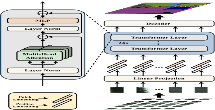
(a)

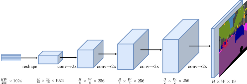
(b)

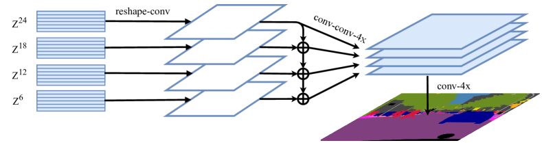
(c)

Figure 1: Schematic illustration of the proposed SEgmentation TRansformer (SETR) (a). We first split an image into fixed-size patches, linearly embed each of them, add position embeddings, and feed the resulting sequence of vectors to a standard Transformer encoder. To perform pixel-wise segmentation, we introduce different decoder designs: (b) progressive upsampling (resulting in a variant called SETR-PUP); and (c) multi-level feature aggregation (a variant called SETR-MLA).

2.1 Semantic segmentation

Semantic segmentation has been significantly boosted by the development of deep neural networks. By removing fully connected layers, a fully convolutional network (FCN) [8] can achieve pixel-wise predictions. While the predictions of FCN are relatively coarse, several CRF/MRF [25, 26, 27] based approaches are developed to help refine the coarse predictions. To address the inherent tension between semantics and location [8], coarse and fine layers need to be aggregated for both the encoder and decoder. This leads to different variants of the encoder-decoder structures [28, 29, 9] for multi-level feature fusion.

Many recent efforts have been focused on addressing the limited receptive field/context modeling problem in FCN. To enlarge the receptive field, DeepLab [30] and Dilation [31] introduce the dilated convolution. Alternatively, context modeling is the focus of PSPNet [14] and DeepLabV2 [32]. The former proposes the PPM module to obtain different region’s contextual information while the latter develops ASPP module that adopts pyramid dilated convolutions with different dilation rates. Decomposed large kernels [11] are also utilized for context capturing. Recently, attention based models are popular for capturing long range context information. PSANet [33] develops the pointwise spatial attention module for dynamically capturing the long range context. DANet [34] embeds both spatial attention and channel attention. CCNet [35] alternatively focuses on economizing the heavy computation budget introduced by full spatial attention. DGMN [36] builds a dynamic graph message passing network for scene modeling and it can significantly reduce the computational complexity. Note that all these approaches are still based on FCNs where the feature encoding and extraction part are based on classical ConvNets like VGG [3] and ResNet [4]. In this work, we alternatively rethink the semantic segmentation task from a different perspective.

2.2 Vision Transformers

Transformers have revolutionized machine translation and NLP [37, 38, 39, 40]. Recently, there are also some explorations for the usage of Transformer structures in image recognition. Non-local network [15] appends Transformer style attention onto the convolutional backbone. AANet [41] mixes convolution and self-attention for backbone training. LRNet [42] and stand-alone networks [43] explore local self-attention to avoid the heavy computation brought by global self-attention. SAN [44] explores two types of self-attention modules. Axial-Attention [18] decomposes the global spatial attention into two separate axial attentions such that the computation is largely reduced. Apart from these pure Transformer based models, there are also CNN-Transformer hybrid ones. DETR [45] and the following deformable version utilize Transformer for object detection where Transformer is appended inside the detection head. STTR [46] and LSTR [47] adopt Transformer for disparity estimation and lane shape prediction respectively. Recently, ViT [1] is the first work to show that a pure Transformer based image classification model can achieve the state-of-the-art. It provides direct inspiration to exploit Transformer based encoder design for semantic segmentation.

The most related work is [18] which also leverages attention for image segmentation. However, there are several key differences. First, though convolution is completely removed in [18] as in our SETR, their model still follows the conventional FCN design in that spatial resolution of feature maps is reduced progressively. In contrast, our prediction model keeps the same spatial resolution throughout and thus represents a step-change in model design. Second, to maximize the scalability on modern hardware accelerators and facilitate easy-to-use, we stick to the standard self-attention design. Instead, [18] adopts a specially designed axial-attention [48] which is less scalable to standard computing facilities. Our model is also superior in segmentation accuracy (see Section 5).

Despite the success of ViTs [1] on coarse classification tasks, more cost-effective variants are necessary for more challenging dense prediction tasks. For example, PVT [49] first introduces spatial reduction attention in a pyramid architecture. CvT [50] similarly coalesces ViTs with convolutional inductive bias. CrossViT [51] instead leverages interaction between large-patch and small-patch branches. Swin [19] shifts the local attention windows to capture global cross-window connection across layers. Recently, Twins [24] combines global attention with efficient local attention. Our HLG Transformer shares a similar spirit as these works by designing a more cost-effective hierarchical local-global Transformer layer.

3 Method

3.1 FCN-based semantic segmentation

In order to contrast with our new model design, let us first revisit the conventional FCN [8] for image semantic segmentation. An FCN encoder consists of a stack of sequentially connected convolutional layers. The first layer takes as input the image, denoted as $H\times W\times 3$ with $H\times W$ specifying the image size in pixels. The input of subsequent layer $i$ is a three-dimensional tensor sized $h\times w\times d$, where $h$ and $w$ are spatial dimensions of feature maps, and $d$ is the feature/channel dimension. Locations of the tensor in a higher layer are computed based on the locations of tensors of all lower layers they are connected to via layer-by-layer convolutions, which are defined as their receptive fields. Due to the locality nature of convolution operation, the receptive field increases linearly along the depth of layers, conditional on the kernel sizes (typically $3\times 3$). As a result, only higher layers with big receptive fields can model long-range dependencies in this FCN architecture. However, it is shown that the benefits of adding more layers would diminish rapidly once reaching certain depths [4]. Having limited receptive fields for context modeling is thus an intrinsic limitation of the vanilla FCN architecture.

Recently, a number of state-of-the-art methods [52, 16, 36] suggest that combing FCN with attention mechanism is a more effective strategy for learning long-range contextual information. These methods limit the attention learning to higher layers with smaller input sizes alone due to its quadratic complexity w.r.tthe pixel number of feature tensors. This means that dependency learning on lower-level feature tensors is lacking, leading to sub-optimal representation learning. To overcome this limitation, we propose a pure self-attention based encoder, named SEgmentation TRansformers (SETR).

3.2 Segmentation Transformers (SETR)

Image to sequence SETR follows the same input-output structure as in NLP for transformation between 1D sequences. There thus exists a mismatch between 2D image and 1D sequence. Concretely, the Transformer, as depicted in Figure 1(a), accepts a 1D sequence of feature embeddings $Z\in\mathbb{R}^{L\times C}$ as input, $L$ is the length of sequence, $C$ is the hidden channel size. Image sequentialization is thus needed to convert an input image $x\in\mathbb{R}^{H\times W\times 3}$ into $Z$.

A straightforward way for image sequentialization is to flatten the image pixel values into a 1D vector with size of $3HW$. For a typical image sized at $480(H)\times 480(W)\times 3$, the resulting vector will have a length of 691,200. Given the quadratic model complexity of Transformer, it is not possible that such high-dimensional vectors can be handled in both space and time. Therefore tokenizing every single pixel as input to our transformer is out of the question.

In view of the fact that a typical encoder designed for semantic segmentation would downsample a 2D image $x\in\mathbb{R}^{H\times W\times 3}$ into a feature map $x_{f}\in\mathbb{R}^{\frac{H}{16}\times\frac{W}{16}\times C}$, we thus decide to set the transformer input sequence length $L$ as $\frac{H}{16}\times\frac{W}{16}=\frac{HW}{256}$. This way, the output sequence of the transformer can be simply reshaped to the target feature map $x_{f}$.

To obtain the $\frac{HW}{256}$-long input sequence, we divide an image $x\in\mathbb{R}^{H\times W\times 3}$ into a grid of $\frac{H}{16}\times\frac{W}{16}$ patches uniformly, and then flatten this grid into a sequence. By further mapping each vectorized patch $p$ into a latent $C$-dimensional embedding space using a linear projection function $f$: $p\longrightarrow e\in\mathbb{R}^{C}$, we obtain a 1D sequence of patch embeddings for an image $x$. To encode the patch spacial information, we learn a specific embedding $p_{i}$ for every location $i$ which is added to $e_{i}$ to form the final sequence input $E=\{e_{1}+p_{1},~{}e_{2}+p_{2},~{}\cdots,~{}e_{L}+p_{L}\}$. This way, spatial information is kept despite the orderless self-attention nature of transformers.

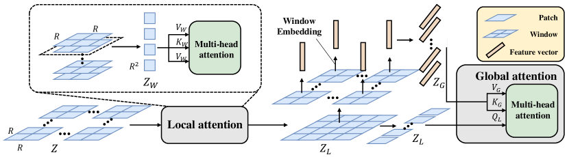
Figure 2: Local-Global attention mechanism. Local attention (in dash line) is applied within each window. Global attention is applied between global feature $Z_{G}$ and local feature $Z_{L}$.

Transformer Given the 1D embedding sequence $E$ as input, a pure transformer based encoder is employed to learn feature representations. This means each transformer layer has a global receptive field, solving the limited receptive field problem of existing FCN encoder once and for all. The transformer encoder consists of $L_{e}$ layers of multi-head self-attention (MSA) and Multilayer Perceptron (MLP) blocks [53] (Figure 1(a)). At each layer $l$, the input to self-attention is in a triplet of (query, key, value) computed from the input $Z^{l-1}\in\mathbb{R}^{L\times C}$ as:

$$\footnotesize\text{query}={Z^{l-1}}\textbf{W}_{Q},\;\text{key}={Z^{l-1}}\textbf{W}_{K},\;\text{value}={Z^{l-1}}\textbf{W}_{V},$$ (1)

where $\textbf{W}_{Q}$/$\textbf{W}_{K}$/$\textbf{W}_{V}\in\mathbb{R}^{C\times d}$ are the learnable parameters of three linear projection layers and $d$ is the dimension of (query, key, value). Self-attention (SA) is then formulated as:

$$\footnotesize SA(Z^{l-1})=Z^{l-1}+\operatorname{softmax}(\frac{Z^{l-1}\textbf{W}_{Q}(Z^{l-1}\textbf{W}_{K})^{\top}}{\sqrt{d}})(Z^{l-1}\textbf{W}_{V}).$$ (2)

MSA is an extension with $m$ independent SA operations and project their concatenated outputs: $MSA(Z^{l-1})=[SA_{1}(Z^{l-1});~{}SA_{2}(Z^{l-1});~{}\cdots;~{}SA_{m}(Z^{l-1})]\textbf{W}_{O}$, where $\textbf{W}_{O}\in\mathbb{R}^{md\times C}$. $d$ is typically set to $C/m$. The output of MSA is then transformed by an MLP block with residual skip as the layer output as:

$$\footnotesize Z^{l}=MSA(Z^{l-1})+MLP(MSA(Z^{l-1}))\in\mathbb{R}^{L\times C}.$$ (3)

Note, layer norm is applied before MSA and MLP blocks which is omitted for simplicity. We denote $\{Z^{1},~{}Z^{2},~{}\cdots,~{}Z^{L_{e}}\}$ as the features of transformer layers.

3.3 Decoder designs

To evaluate the effectiveness of SETR’s encoder feature representations $Z$, we introduce three different decoder designs to perform pixel-level segmentation. As the goal of the decoder is to generate the segmentation results in the original 2D image space $(H\times W)$, we need to reshape the encoder’s features (that are used in the decoder), $Z$, from a 2D shape of $\frac{HW}{256}\times C$ to a standard 3D feature map $\frac{H}{16}\times\frac{W}{16}\times C$. Next, we briefly describe the three decoders.

(1) Naive upsampling (Naive) This naive decoder first projects the transformer feature $Z^{L_{e}}$ to the dimension of category number (e.g., 19 for experiments on Cityscapes). For this we adopt a simple 2-layer network with architecture: $1\times 1$ conv + sync batch norm (w/ ReLU) + $1\times 1$ conv. After that, we simply bilinearly upsample the output to the full image resolution, followed by a classification layer with pixel-wise cross-entropy loss. When this decoder is used, we denote our model as SETR-Naïve.

(2) Progressive UPsampling (PUP) Instead of one-step upscaling which may introduce noisy predictions, we consider a progressive upsampling strategy that alternates conv layers and upsampling operations. To maximally mitigate the adversarial effect, we restrict upsampling to 2$\times$. Hence, a total of 4 operations are needed for reaching the full resolution from $Z^{L_{e}}$ with size $\frac{H}{16}\times\frac{W}{16}$. More details of this process are given in Figure 1(b). When using this decoder, we denote our model as SETR-PUP.

(3) Multi-Level feature Aggregation (MLA)

The third design is characterized by multi-level feature aggregation (Figure 1(c)) in similar spirit of feature pyramid network [54, 55]. However, our decoder is fundamentally different because the feature representations $Z^{l}$ of every SETR’s layer share the same resolution without a pyramid shape.

Specifically, we take as input the feature representations $\{Z^{m}\}$ ($m\in\{{\frac{L_{e}}{M}},{2\frac{L_{e}}{M}},\cdots,{M\frac{L_{e}}{M}}\}$) from $M$ layers uniformly distributed across the layers with step $\frac{L_{e}}{M}$ to the decoder. $M$ streams are then deployed, with each focusing on one specific selected layer. In each stream, we first reshape the encoder’s feature $Z^{l}$ from a 2D shape of $\frac{HW}{256}\times C$ to a 3D feature map $\frac{H}{16}\times\frac{W}{16}\times C$. A 3-layer (kernel size $1\times 1$, $3\times 3$, and $3\times 3$) network is applied with the feature channels halved at the first and third layers respectively, and the spatial resolution upscaled $4\times$ by bilinear operation after the third layer. To enhance the interactions across different streams, we introduce a top-down aggregation design via element-wise addition after the first layer. An additional $3\times 3$ conv is applied after the element-wise additioned feature. After the third layer, we obtain the fused feature from all the streams via channel-wise concatenation which is then bilinearly upsampled $4\times$ to the full resolution. When using this decoder, we denote our model as SETR-MLA.

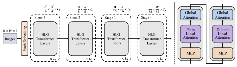
Figure 3: Left: Hierarchical local-global Transformers backbone architecture. Right: Successive hierarchical local-global Transformer layer.

4 Hierarchical Local-Global (HLG)

4.1 Overview

As a conventional ViT [1] learns feature representation of a single resolution with quadratic computation complexity w.r.t the input image size, it is not appropriate to be a backbone network to support various fine downstream tasks, e.g., object detection and instance segmentation. In this paper, we introduce a family of Hierarchical Local-Global (HLG) Transformers in a pyramidal structure, serving as a general-purpose backbone network. An overview of our HLG architecture is depicted in Figure 3. A HLG model consists of four stages for multi-scale feature representation learning. Specifically, an input image is first fed to the patch embedding module and downsampled by overlapping patch divisions, followed by $L_{i}$ HLG layers with $i$ the stage index. All stages share the same structure including one patch embedding module and multiple encoding modules. The output size of each stage $x_{f}^{0},x_{f}^{1},x_{f}^{2},x_{f}^{3}$ is designated to be $\frac{H}{4}\times\frac{W}{4}$, $\frac{H}{8}\times\frac{W}{8}$, $\frac{H}{16}\times\frac{W}{16}$, $\frac{H}{32}\times\frac{W}{32}$ sequentially. Next, we describe the key design of the proposed HLG Transformer layer.

4.2 Local-Global attention

An illustration of our local-global attention is given at Figure 2. Local attention Given an input feature map $Z$ of size $N_{h}\times N_{w}$, it is first divided into $\frac{N_{h}\times N_{w}}{R^{2}}$ windows in a non-overlapping manner, where $R\times R$ represents the window size. The multi-head self-attention is then applied within each local window $Z_{W}\in\mathbb{R}^{R\times R\times C}$. The attention operation can be expressed as:

$$Q_{W}=Z_{W}\mathbf{W}^{(L)}_{Q},K_{W}=Z_{W}\mathbf{W}^{(L)}_{K},V_{W}=Z_{W}\mathbf{W}^{(L)}_{V}$$ (4)

$$\text{SA}(Z_{W})=Z_{W}+\text{softmax}\left(\frac{Q_{W}K^{\top}_{W}}{\sqrt{d}}+B_{W}\right)V_{W},$$ (5)

where $\mathbf{W}^{(L)}_{Q},\mathbf{W}^{(L)}_{K},\mathbf{W}^{(L)}_{V}\in\mathbb{R}^{C\times d}$ are learnable parameters of three linear projection layers shared by all windows and $d$ is the dimension of $Q_{W},Q_{K},Q_{V}$. $B_{W}\in\mathbb{R}^{R^{2}\times R^{2}}$ is local relative positional encoding. Then we assemble each window feature back to obtain the local feature map $Z_{L}\in\mathbb{R}^{N_{h}\times N_{W}\times C}$. This plain local attention can be achieved by non-overlapping window division with focus on information exchange between spatially adjacent patches (Figure 4 left). This scheme is however limited to short range interaction within each individual window. To enable long range dependency discovery without extra computation cost, we further introduce a dilated local attention mechanism for stronger representation learning (Figure 4 right). In particular, we form anther type of window by sampling patches in a spaced manner, e.g., sampling a patch every three positions as illustrated in (Figure 4). This allows to learn a relatively longer range dependency using efficient local attention.

Global attention Following local feature map $Z_{L}$, we further design an efficient global attention for holistic context learning. To that end, we introduce a Window Embedding operation that extracts an 1-dimensional feature vector $\mathbb{R}^{1\times 1\times C}$ per window. Window embedding operations can be implemented by depth-wise convolution [56], average pooling or max pooling with kernel size and stride equal to the window size. Empirically we find average pooling is generally effective for downstream tasks. More details will be discussed in the experiments. As a result, a compact global feature map $Z_{G}\in\mathbb{R}^{\frac{N_{h}}{R}\times\frac{N_{w}}{R}}\times C$ can be obtained. Global attention is then applied to feature map $Z_{L}$ and $Z_{G}$. This enables efficient global attention by querying $Z_{L}$ towards $Z_{G}$ formulated as:

$$Q_{L}=Z_{L}\mathbf{W}^{(G)}_{Q},\quad K_{G}=Z_{G}\mathbf{W}^{(G)}_{K},\quad V_{G}=Z_{G}\mathbf{W}^{(G)}_{V}$$ (6)

$$\text{SA}(Z_{L},Z_{G})=Z_{L}+\text{softmax}\left(\frac{Q_{L}K_{G}^{\top}}{\sqrt{d}}+B_{G}\right)V_{G},$$ (7)

where $\mathbf{W}^{(G)}_{Q},\mathbf{W}^{(G)}_{K},\mathbf{W}^{(G)}_{V}\in\mathbb{R}^{C\times d}$ are learnable parameters of three linear projection layers and $d$ is the dimension of $Q_{W},Q_{K},Q_{V}$. $B_{G}\in\mathbb{R}^{(N_{h}\times N_{w})\times(\frac{N_{h}}{R}\times\frac{N_{w}}{R})}$ is global relative positional encoding.

Parameter and computation sharing For further efficiency, we propose to share the parameters and computation between local and global attention. Concretely, all the parameters of local and global attention are shared as

$$\mathbf{W}^{(L)}_{Q}=\mathbf{W}^{(G)}_{Q},\mathbf{W}^{(L)}_{K}=\mathbf{W}^{(G)}_{K},\mathbf{W}^{(L)}_{V}=\mathbf{W}^{(G)}_{V}$$ (8)

Computation sharing is non-trivial. To that end, we replace $Z_{L}$ of Eq. (6) with the output of Eq. (5) as:

$$Q_{L} =\left(Z_{W}+\text{softmax}\left(\frac{Q_{W}K^{\top}_{W}}{\sqrt{d}}+B_{W}\right)V_{W}\right)\mathbf{W}^{(G)}_{Q}$$

$$=Z_{W}W_{Q}^{(L)}+\text{softmax}\left(\frac{Q_{W}K^{\top}_{W}}{\sqrt{d}}+B_{W}\right)V_{W}\mathbf{W}^{(G)}_{Q}$$

As a result, we achieve the the first term by reusing Eq. (4), and the second term by a computation-friendly depth-with convolution as

$$Q_{L}=Q_{W}+\text{DWConv}\left(V_{W}\right)$$ (9)

where $Q_{W}$ and $K_{W}$ are shared with local attention.

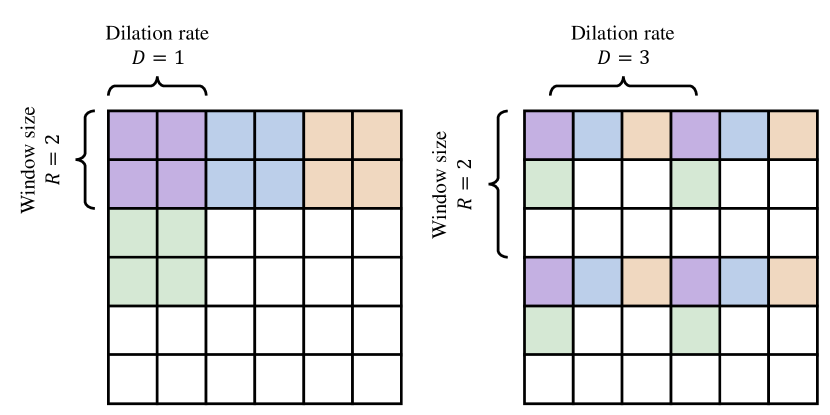
Figure 4: Left: plain local attention; Right: dilated local attention.

DWMLP Following [57, 58], we implement our MLP with a depth-wise convolution and squeeze-and-excitation [59]. We place the MLP before attention so that downsampling can be achieved simply by setting the stride of MLP (first layer in each stage) as 2.

4.3 Hierarchical Local-Global Transformer layer

To facilitate synergistic interaction without extra complexity and computational cost, we intertwine the plain and dilated local attention sequentially. Both use the same window size. This attention cascading design results in our Hierarchical Local-Global (HLG) Transformer layer (Figure 3 right).

4.4 Architecture design

Table 1: Architecture specifications of HLG. $Conv3\times 3$ means the convolution with a kernel size of $3\times 3$, $Conv1\times 1$ denotes the convolution with a kernel size of $1\times 1$, and $DWConv3\times 3$ represents the depth-wise convolution with a kernel size of $3\times 3$.

Output	HLG-Mobile	HLG-Tiny	HLG-Small	HLG-Medium	HLG-Large
$56\times 56$	$Conv3\times 3(stride=2),Conv1\times 1,Conv3\times 3(stride=2)$
	${\begin{bmatrix}C_{1}=48\\ H_{1}=2\\ R_{1}=7\\ D_{1}=8\\ \end{bmatrix}}\times 2$	${\begin{bmatrix}C_{1}=64\\ H_{1}=2\\ R_{1}=7\\ D_{1}=8\\ \end{bmatrix}}\times 2$	${\begin{bmatrix}C_{1}=96\\ H_{1}=3\\ R_{1}=7\\ D_{1}=8\\ \end{bmatrix}}\times 2$	${\begin{bmatrix}C_{1}=96\\ H_{1}=3\\ R_{1}=7\\ D_{1}=8\\ \end{bmatrix}}\times 2$	${\begin{bmatrix}C_{1}=128\\ H_{1}=4\\ R_{1}=7\\ D_{1}=8\\ \end{bmatrix}}\times 2$
$28\times 28$	$DWConv3\times 3(stride=2)$
	${\begin{bmatrix}C_{2}=96\\ H_{2}=4\\ R_{2}=7\\ D_{2}=4\\ \end{bmatrix}}\times 2$	${\begin{bmatrix}C_{2}=128\\ H_{2}=4\\ R_{2}=7\\ D_{2}=4\\ \end{bmatrix}}\times 2$	${\begin{bmatrix}C_{2}=192\\ H_{2}=6\\ R_{2}=7\\ D_{2}=4\\ \end{bmatrix}}\times 2$	${\begin{bmatrix}C_{2}=192\\ H_{2}=6\\ R_{2}=7\\ D_{2}=4\\ \end{bmatrix}}\times 2$	${\begin{bmatrix}C_{2}=256\\ H_{2}=8\\ R_{2}=7\\ D_{2}=4\\ \end{bmatrix}}\times 2$
$14\times 14$	$DWConv3\times 3(stride=2)$
	${\begin{bmatrix}C_{3}=192\\ H_{3}=8\\ R_{3}=7\\ D_{3}=2\\ \end{bmatrix}}\times 2$	${\begin{bmatrix}C_{3}=256\\ H_{3}=8\\ R_{3}=7\\ D_{3}=2\\ \end{bmatrix}}\times 6$	${\begin{bmatrix}C_{3}=384\\ H_{3}=12\\ R_{3}=7\\ D_{3}=2\\ \end{bmatrix}}\times 6$	${\begin{bmatrix}C_{3}=384\\ H_{3}=12\\ R_{3}=7\\ D_{3}=2\\ \end{bmatrix}}\times 14$	${\begin{bmatrix}C_{3}=512\\ H_{3}=16\\ R_{3}=7\\ D_{3}=2\\ \end{bmatrix}}\times 14$
$7\times 7$	$DWConv3\times 3(stride=2)$
	${\begin{bmatrix}C_{4}=384\\ H_{4}=16\\ R_{4}=7\\ D_{4}=1\\ \end{bmatrix}}\times 2$	${\begin{bmatrix}C_{4}=512\\ H_{4}=16\\ R_{4}=7\\ D_{4}=1\\ \end{bmatrix}}\times 2$	${\begin{bmatrix}C_{4}=768\\ H_{4}=24\\ R_{4}=7\\ D_{4}=1\\ \end{bmatrix}}\times 2$	${\begin{bmatrix}C_{4}=768\\ H_{4}=24\\ R_{4}=7\\ D_{4}=1\\ \end{bmatrix}}\times 2$	${\begin{bmatrix}C_{4}=1024\\ H_{4}=32\\ R_{4}=7\\ D_{4}=1\\ \end{bmatrix}}\times 2$

Table 1 summarizes the family of our HLG Transformers with a variety of capacities, including HLG-Mobile, -Tiny, -Small, -Medium, -Large. The hyper-parameters are explained as follows:

• $C_{i}$: The embedding dimension of each stage $i$;

• $H_{i}$: The number of head in stage $i$;

• $R_{i}$: The window size of local attention;

• $D_{i}$: The dilation rate of local attention.

4.5 HLG Segmentation Transformers

We detail the integration of HLG for segmentation. To align with the input format (i.e., a spatial shape of $\frac{H}{16}\times\frac{W}{16}$) of SETR decoder, we interpolate the features of all four stages to this shape, followed by concatenating and transforming them into a single tensor. The decoder uses a pair of HLG Transformer layers with plain and dilated local attention with the window size $R$ set to $8$. The segmentation result is obtained by Progressive UPsampling (PUP).

5 Experiments on SETR

Table 2: Configuration of SETR backbone variants.

Model	T-layers	Hidden size	Att head
T-Base	12	768	12
T-Large	24	1024	16

Table 3: Comparing SETR variants on different pre-training strategies and backbones. All experiments are trained on Cityscapes train fine set with batch size 8, and evaluated using the single scale test protocol on the Cityscapes validation set in mean IoU (%) rate. “Pre” denotes the pre-training of Transformer part. “R” means the Transformer part is randomly initialized.

Method	Pretrain	Backbone	#Params	40k	80k
FCN [60]	1K	R-101	68.59M	73.93	75.52
Semantic FPN [60]	1K	R-101	47.51M	-	75.80
Hybrid-Base	R	T-Base	112.59M	74.48	77.36
Hybrid-Base	21K	T-Base	112.59M	76.76	76.57
Hybrid-DeiT	21K	T-Base	112.59M	77.42	78.28
SETR-Naïve	21K	T-Large	305.67M	77.37	77.90
SETR-MLA	21K	T-Large	310.57M	76.65	77.24
SETR-PUP	21K	T-Large	318.31M	78.39	79.34
SETR-PUP	R	T-Large	318.31M	42.27	-
SETR-Naïve-Base	21K	T-Base	87.69M	75.54	76.25
SETR-MLA-Base	21K	T-Base	92.59M	75.60	76.87
SETR-PUP-Base	21K	T-Base	97.64M	76.71	78.02
SETR-Naïve-DeiT	1K	T-Base	87.69M	77.85	78.66
SETR-MLA-DeiT	1K	T-Base	92.59M	78.04	78.98
SETR-PUP-DeiT	1K	T-Base	97.64M	78.79	79.45
SETR-MLA-BEiT	21K	T-Large	310.57M	79.59	80.20
SETR-PUP-BEiT	21K	T-Large	318.31M	79.84	80.43

5.1 Experimental setup

We conduct experiments on three representative semantic segmentation benchmark datasets.

Cityscapes [61] densely annotates 19 object categories in images with urban scenes. It contains 5000 finely annotated images, split into 2975,  500 and 1525 for training, validation and testing respectively. The images are all captured at a high resolution of $2048\times 1024$. In addition, it provides 19,998 coarse annotated images for model training.

ADE20K [62] is a challenging scene parsing benchmark with 150 fine-grained semantic concepts. It contains 20210,  2000 and 3352 images for training, validation and testing.

PASCAL Context [63] provides pixel-wise semantic labels for the whole scene (both “thing” and “stuff” classes), and contains 4998 and 5105 images for training and validation respectively. Following previous works, we evaluate on the most frequent 59 classes and the background class (60 classes in total).

Table 4: Comparison to FCN with different pre-training with single-scale inference on the ADE20K val and Cityscapes val set.

Method	Pre	Backbone	ADE20K	Cityscapes
FCN  [60]	1K	R-101	39.91	73.93
FCN	21K	R-101	42.17	76.38
SETR-MLA	21K	T-Large	48.64	76.65
SETR-PUP	21K	T-Large	48.58	78.39
SETR-MLA-DeiT	1K	T-Large	46.15	78.98
SETR-PUP-DeiT	1K	T-Large	46.24	79.45

Implementation details Following the default setting (e.g., data augmentation and training schedule) of public codebase mmsegmentation [60], (i) we apply random resize with ratio between 0.5 and 2, random cropping (768, 512 and 480 for Cityscapes, ADE20K and Pascal Context respectively) and random horizontal flipping during training for all the experiments; (ii) We set batch size 16 and the total iteration to 160,000 and 80,000 for the experiments on ADE20K and Pascal Context. For Cityscapes, we set batch size to 8 with a number of training schedules reported in Table 3, 7 and 8 for fair comparison. We adopt a polynomial learning rate decay schedule [14] and employ SGD as the optimizer. Momentum and weight decay are set to 0.9 and 0 respectively for all the experiments on the three datasets. We set initial learning rate 0.001 on ADE20K and Pascal Context, and 0.01 on Cityscapes.

Auxiliary loss As [14] we also find the auxiliary segmentation loss helps the model training. Each auxiliary loss head follows a 2-layer network. We add auxiliary losses at different Transformer layers: SETR-Naïve ($Z^{10},Z^{15},Z^{20}$), SETR-PUP ($Z^{10},Z^{15},Z^{20},Z^{24}$), SETR-MLA ($Z^{6},Z^{12},Z^{18},Z^{24}$). Both auxiliary loss and main loss heads are applied concurrently.

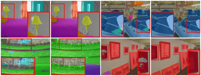
Figure 5: Qualitative results on ADE20K: SETR (right column) vs. dilated FCN baseline (left column) in each pair. Best viewed in color and zoom in.

Table 5: State-of-the-art comparison on the ADE20K dataset. Performances of different model variants are reported. SS: Single-scale inference. MS: Multi-scale inference.

Method	Pre	Backbone	#Params	mIoU
FCN (160k, SS) [60]	1K	ResNet-101	68.59M	39.91
FCN (160k, MS) [60]	1K	ResNet-101	68.59M	41.40
CCNet [16]	1K	ResNet-101	-	45.22
Strip pooling [64]	1K	ResNet-101	-	45.60
DANet [34]	1K	ResNet-101	69.0M	45.30
OCRNet [65]	1K	ResNet-101	71.0M	45.70
UperNet [66]	1K	ResNet-101	86.0M	44.90
Deeplab V3+ [67]	1K	ResNet-101	63.0M	46.40
SETR-Naïve (160k, SS)	21K	T-Large	305.67M	48.06
SETR-Naïve (160k, MS)	21K	T-Large	305.67M	48.80
SETR-PUP (160k, SS)	21K	T-Large	318.31M	48.58
SETR-PUP (160k, MS)	21K	T-Large	318.31M	50.09
SETR-MLA (160k, SS)	21K	T-Large	310.57M	48.64
SETR-MLA (160k, MS)	21K	T-Large	310.57M	50.28
SETR-PUP-DeiT (160k, SS)	1K	T-Base	97.64M	46.34
SETR-PUP-DeiT (160k, MS)	1K	T-Base	97.64M	47.30
SETR-MLA-DeiT (160k, SS)	1K	T-Base	92.59M	46.15
SETR-MLA-DeiT (160k, MS)	1K	T-Base	92.59M	47.71
SETR-PUP-BEiT (160k, SS)	21K	T-Large	318.31M	52.54$\pm$0.4
SETR-PUP-BEiT (160k, MS)	21K	T-Large	318.31M	52.74$\pm$0.4
SETR-MLA-BEiT (160k, SS)	21K	T-Large	318.31M	53.03$\pm$0.4
SETR-MLA-BEiT (160k, MS)	21K	T-Large	318.31M	53.13$\pm$0.4

Multi-scale test We use the default settings of mmsegmentation [60]. Specifically, the input image is first scaled to a uniform size. Multi-scale scaling and random horizontal flip are then performed on the image with a scaling factor (0.5, 0.75, 1.0, 1.25, 1.5, 1.75). Sliding window is adopted for test (e.g., $480\times 480$ for Pascal Context). If the shorter side is smaller than the size of the sliding window, the image is scaled with its shorter side to the size of the sliding window (e.g., 480) while keeping the aspect ratio. Synchronized BN is used in decoder and auxiliary loss heads. For training simplicity, we do not adopt the widely-used tricks such as OHEM [68] loss in model training.

Baselines We adopt dilated FCN [8] and Semantic FPN [55] as baselines with their results taken from [60]. Our models and the baselines are trained and tested in the same settings for fair comparison. In addition, state-of-the-art models are also compared. Note that the dilated FCN is with output stride 8 and we use output stride 16 in all our models due to GPU memory constrain.

SETR variants

Three variants of our model with different decoder designs (see Sec. 3.3), namely SETR-Naïve, SETR-PUP  and SETR-MLA. Besides, we use two variants of the encoder “T-Base” and “T-Large” with 12 and 24 layers respectively (Table 2). Unless otherwise specified, we use “T-Large” as the encoder for SETR-Naïve, SETR-PUP and SETR-MLA. We denote SETR-Naïve-Base as the model utilizing “T-Base” in SETR-Naïve.

Though designed as a model with a pure Transformer encoder, we also set a hybrid baseline Hybrid by using a ResNet-50 based FCN encoder and feeding its output feature into SETR. To cope with the GPU memory constraint and for fair comparison, we only consider ‘T-Base” in Hybrid and set the output stride of FCN to $1/16$. That is, Hybrid  is a combination of ResNet-50 and SETR-Naïve-Base.

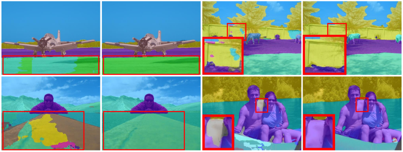
Figure 6: Qualitative results on Pascal Context: SETR (right column) vs. dilated FCN baseline (left column) in each pair. Best viewed in color and zoom in.

Table 6: State-of-the-art comparison on the Pascal Context dataset. Performances of different model variants are reported. SS: Single-scale inference. MS: Multi-scale inference.

Method	Pre	Backbone	mIoU
FCN (80k, SS) [60]	1K	ResNet-101	44.47
FCN (80k, MS) [60]	1K	ResNet-101	45.74
DANet [34]	1K	ResNet-101	52.60
EMANet [69]	1K	ResNet-101	53.10
SVCNet [70]	1K	ResNet-101	53.20
Strip pooling [64]	1K	ResNet-101	54.50
GFFNet [71]	1K	ResNet-101	54.20
APCNet [72]	1K	ResNet-101	54.70
SETR-Naïve (80k, SS)	21K	T-Large	52.89
SETR-Naïve (80k, MS)	21K	T-Large	53.61
SETR-PUP (80k, SS)	21K	T-Large	54.40
SETR-PUP (80k, MS)	21K	T-Large	55.27
SETR-MLA (80k, SS)	21K	T-Large	54.87
SETR-MLA (80k, MS)	21K	T-Large	55.83
SETR-PUP-DeiT (80k, SS)	1K	T-Base	52.71
SETR-PUP-DeiT (80k, MS)	1K	T-Base	53.71
SETR-MLA-DeiT (80k, SS)	1K	T-Base	52.91
SETR-MLA-DeiT (80k, MS)	1K	T-Base	53.74

Pre-training We use the pre-trained weights provided by ViT [1], DeiT [73] or BEiT [74] to initialize all the Transformer layers and the input linear projection layer in our model. We denote SETR-Naïve-DeiT as the model utilizing DeiT [73] pre-training in SETR-Naïve-Base and SETR-PUP-BEiT as the model model utilizing BEiT [74] pre-training in SETR-PUP. All the layers without pre-training are randomly initialized. For the FCN encoder of Hybrid, we use the initial weights pre-trained on ImageNet-1k. For the Transformer part, we use the weights pre-trained by ViT [1], DeiT [73], BEiT [74] or randomly initialized.

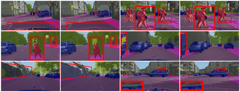
Figure 7: Qualitative results on Cityscapes: SETR (right column) vs. dilated FCN baseline (left column) in each pair. Best viewed in color and zoom in.

Table 7: State-of-the-art comparison on the Cityscapes validation set. Performances of different training schedules (e.g., 40k and 80k) are reported. SS: Single-scale inference. MS: Multi-scale inference.

Method	Backbone	mIoU
FCN (40k, SS) [60]	ResNet-101	73.93
FCN (40k, MS) [60]	ResNet-101	75.14
FCN (80k, SS) [60]	ResNet-101	75.52
FCN (80k, MS) [60]	ResNet-101	76.61
PSPNet [14]	ResNet-101	78.50
DeepLab-v3 [75] (MS)	ResNet-101	79.30
NonLocal [15]	ResNet-101	79.10
CCNet [16]	ResNet-101	80.20
GCNet [76]	ResNet-101	78.10
Axial-DeepLab-XL [18] (MS)	Axial-ResNet-XL	81.10
Axial-DeepLab-L [18] (MS)	Axial-ResNet-L	81.50
SETR-PUP (40k, SS)	T-Large	78.39
SETR-PUP (40k, MS)	T-Large	81.57
SETR-PUP (80k, SS)	T-Large	79.34
SETR-PUP (80k, MS)	T-Large	82.15

We use patch size $16\times 16$ for all the experiments. We perform 2D interpolation on the pre-trained position embeddings, according to their location in the original image for different input size fine-tuning.

Evaluation metric Following the standard evaluation protocol [61], the metric of mean Intersection over Union (mIoU) averaged over all classes is reported. For ADE20K, additionally pixel-wise accuracy is reported following the existing practice.

5.2 Ablation studies

Table 3 and 4 show ablation studies on (a) different variants of SETR on various training schedules, (b) comparison to FCN [60] and Semantic FPN [60], (c) pre-training on different data, (d) comparison with Hybrid, and (e) comparison to FCN with different pre-training. Unless specified otherwise, all experiments in Table 3 and 4 are trained on Cityscapes train fine set with batch size 8, and evaluated using the single scale test protocol on the Cityscapes validation set in mean IoU (%) rate. Experiments on ADE20K also follow the single scale test protocol.

Table 8: Comparison on the Cityscapes test set. ${\ddagger}$: trained on fine and coarse annotated data.

Method	Backbone	mIoU
PSPNet [14]	ResNet-101	78.40
DenseASPP [10]	DenseNet-161	80.60
BiSeNet [77]	ResNet-101	78.90
PSANet [33]	ResNet-101	80.10
DANet [34]	ResNet-101	81.50
OCNet [68]	ResNet-101	80.10
CCNet [16]	ResNet-101	81.90
Axial-DeepLab-L [18]	Axial-ResNet-L	79.50
Axial-DeepLab-XL [18]	Axial-ResNet-XL	79.90
SETR-PUP (100k)	T-Large	81.08
SETR-PUP‡	T-Large	81.64

From Table 3, we can make the following observations: (i) Progressively upsampling the feature maps, SETR-PUP achieves the best performance among all the variants on Cityscapes. One possible reason for inferior performance of SETR-MLA is that the feature outputs of different Transformer layers do not have the benefits of resolution pyramid as in feature pyramid network (FPN) (see Figure 8). However, SETR-MLA performs slightly better than SETR-PUP, and much superior to the variant SETR-Naïve that upsamples the Transformers output feature by 16$\times$ in one-shot, on ADE20K val set (Table 4 and 5). (ii) The variants using “T-Large” (e.g., SETR-MLA and SETR-Naïve) are superior to their “T-Base” counterparts, i.e., SETR-MLA-Base and SETR-Naïve-Base, as expected. (iii) While our SETR-PUP-Base (76.71) performs worse than Hybrid-Base (76.76), it shines (78.02) when training with more iterations (80k). It suggests that FCN encoder design can be replaced in semantic segmentation, and further confirms the effectiveness of our model. (iv) Pre-training is critical for our model. Randomly initialized SETR-PUP only gives 42.27% mIoU on Cityscapes. Model pre-trained with BEiT [74] on ImageNet-1K gives the best performance on Cityscapes, surpassing the alternative pre-trained with ViT [1] on ImageNet-21K. (v) To study the power of pre-training and further verify the effectiveness of our proposed approach, we conduct the ablation study on the pre-training strategy. For fair comparison with the FCN baseline, we first pre-train a ResNet-101 on the ImageNet-21k dataset with a classification task and then adopt the pre-trained weights for a dilated FCN training for semantic segmentation on the target dataset (ADE20K or Cityscapes). As shown in Table 4, with ImageNet-21k pre-training the FCN baseline experiences a clear improvement over the variant pre-trained on ImageNet-1k. However, our method outperforms the FCN counterparts by a large margin, verifying that the advantage largely comes from the proposed sequence-to-sequence representation learning strategy rather than bigger pre-training data.

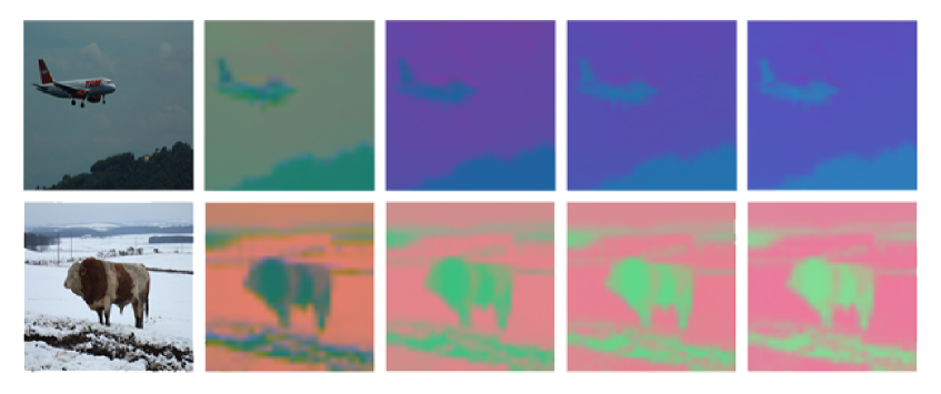
Figure 8: Visualization of output feature of layer $Z^{1}$, $Z^{9}$, $Z^{17}$, $Z^{24}$ of SETR trained on Pascal Context. Best viewed in color.

5.3 Comparison to the state of the art

Results on ADE20K Table 5 presents our results on the more challenging ADE20K dataset. Our SETR-MLA achieves superior mIoU of 48.64% with single-scale (SS) inference. When multi-scale inference is adopted, our method achieves a new state of the art with mIoU hitting 50.28%. Figure 5 shows the qualitative results of our model and dilated FCN on ADE20K. When training a single model on the train+validation set with the default 160,000 iterations, our method ranks $1^{st}$ place in the highly competitive ADE20K test server leaderboard.

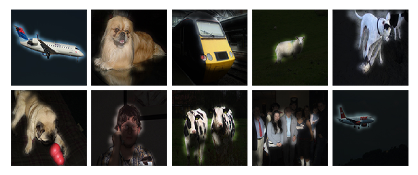
Figure 9: Examples of attention maps from SETR trained on Pascal Context.

Results on Pascal Context Table 6 compares the segmentation results on Pascal Context. Dilated FCN with the ResNet-101 backbone achieves a mIoU of 45.74%. Using the same training schedule, our proposed SETR significantly outperforms this baseline, achieving mIoU of 54.40% (SETR-PUP) and 54.87% (SETR-MLA). SETR-MLA further improves the performance to 55.83% when multi-scale (MS) inference is adopted, outperforming the nearest rival APCNet with a clear margin. Figure 6 gives some qualitative results of SETR and dilated FCN. Further visualization of the learned attention maps in Figure 9 shows that SETR can attend to semantically meaningful foreground regions, demonstrating its ability to learn discriminative feature representations useful for segmentation.

Results on Cityscapes Tables 7 and 8 show the comparative results on the validation and test set of Cityscapes respectively. We can see that our model SETR-PUP is superior to FCN baselines, and FCN plus attention based approaches, such as Non-local [15] and CCNet [16]; and its performance is on par with the best results reported so far. On this dataset we can now compare with the closely related Axial-DeepLab [78, 18] which aims to use an attention-alone model but still follows the basic structure of FCN. Note that Axial-DeepLab sets the same output stride 16 as ours. However, its full input resolution ($1024\times 2048$) is much larger than our crop size $768\times 768$, and it runs more epochs (60k iteration with batch size 32) than our setting (80k iterations with batch size 8). Nevertheless, our model is still superior to Axial-DeepLab when multi-scale inference is adopted on Cityscapes validation set. Using the fine set only, our model (trained with 100k iterations) outperforms Axial-DeepLab-XL with a clear margin on the test set. Figure 7 shows the qualitative results of our model and dilated FCN on Cityscapes.

6 Experiments on HLG

In this section, we focus on the evaluation of the proposed HLG Transformers. We first evaluate the image classification task using our HLG Transformers as the backbone. For more extensive and task agnostic evaluations, we further test object detection, instance segmentation, and semantic segmentation.

6.1 Image classification

Dataset

The ImageNet-1K dataset [79] contains 1.28 million training images and 50K validation images from 1,000 object categories used for model training and evaluation respectively.

Implementation details

We validate the performance of a HLG Transformer by training on the training set and reporting the Top-1 accuracy on the validation set. For a fair comparison, we follow the setting of Swin Transformer [19] and DeiT [73]. For data augmentation, we perform random-size cropping to $224\times 224$, and adopt random horizontal flipping [5] and mix up [80]. Training from scratch, we set the batch size to 1024 and the epochs to 300. We use an initialization learning rate of 0.001, a cosine decay learning rate scheduler with 20 epochs of linear warm-up. We employ the AdamW optimizer with a weight decay 0f 0.05. To prevent model overfitting, the drop-path [81] rate is set to 0.1 by default and 0.3 for HLG-Large due to its stronger capacity.

Results on ImageNet

Table 9: State-of-the-art comparison on the ILSVRC-2012 ImageNet-1K validation dataset. Performances of different model variants are reported.

Method	Image size	#Params	FLOPs	Top1(%)
DeiT-Ti [73]	$224^{2}$	5.7M	1.3G	72.2
CrossViT-Ti [51]	$224^{2}$	6.9M	1.6G	73.4
HLG-Mobile	$224^{2}$	4.3M	0.9G	75.1
PiT-XS  [82]	$224^{2}$	10.6M	1.4G	78.1
ConT-S  [83]	$224^{2}$	10.1M	1.5G	76.5
PVT-T  [49]	$224^{2}$	13.2M	1.9G	75.1
ConViT-Ti+  [23]	$224^{2}$	10.0M	2.0G	76.7
ViP-Ti  [84]	$224^{2}$	12.8M	1.7G	79.0
HLG-Tiny	$224^{2}$	11.0M	2.1G	81.1
LocalViT-S  [22]	$224^{2}$	22.4M	4.6G	80.8
ConViT-S  [23]	$224^{2}$	27.0M	5.4G	81.3
NesT-S  [85]	$224^{2}$	17.0M	5.8G	81.5
Swin-T  [19]	$224^{2}$	29.0M	4.5G	81.3
CoAtNet-0 [86]	$224^{2}$	25.0M	4.2G	81.6
DeiT III-S [87]	$224^{2}$	22.0M	4.6G	81.4
SwinV2-T [88]	$256^{2}$	29.0M	4.5G	81.7
ConvNext-T [89]	$224^{2}$	29.0M	4.5G	82.1
HLG-Small	$224^{2}$	24.2M	4.7G	82.3
ConT-M  [83]	$224^{2}$	39.6M	6.4G	81.8
Twins-PCPVT-B  [24]	$224^{2}$	43.8M	6.4G	82.7
PVT-M  [49]	$224^{2}$	44.2M	6.7G	81.2
Swin-S  [19]	$224^{2}$	50.0M	8.7G	83.0
ConvNext-S  [89]	$224^{2}$	50.0M	8.7G	83.1
CoAtNet-1 [86]	$224^{2}$	42.0M	8.4G	83.3
SwinV2-S  [88]	$256^{2}$	50.0M	8.7G	83.6
HLG-Medium	$224^{2}$	43.7M	9.0G	83.6
DeiT-B  [73]	$224^{2}$	86.6M	17.6G	81.8
PiT-B  [82]	$224^{2}$	73.8M	12.5G	82.0
ConViT-B  [23]	$224^{2}$	86.0M	17.0G	82.4
Swin-B  [19]	$224^{2}$	88.0M	15.4G	83.3
DeiT III-B [87]	$224^{2}$	86.6M	15.5G	83.8
ConvNext-S  [89]	$224^{2}$	89.0M	15.4G	83.8
CoAtNet-2 [86]	$224^{2}$	75.0M	15.7G	84.1
SwinV2-B  [88]	$256^{2}$	88.0M	15.4G	84.1
HLG-Large	$224^{2}$	84.2M	15.9G	84.1

Table 10: Throughput, peek memory and image classification results on ImageNet-1K V2 [90] matched frequency dataset.

Method	Size	#Params	FLOPs	FPS	Memory	Top1 (%)
Swin-T	$224^{2}$	29M	4.5G	755	11.6GB	69.7
Swin-S	$224^{2}$	50M	8.7G	437	18.6GB	72.1
Swin-B	$224^{2}$	88M	15.4G	278	25.2GB	72.3
HLG-Tiny	$224^{2}$	11M	2.1G	734	11.7GB	70.1
HLG-Small	$224^{2}$	24M	4.7G	697	17.5GB	70.3
HLG-Medium	$224^{2}$	44M	9.0G	392	23.6GB	72.4
HLG-Large	$224^{2}$	84M	15.9G	221	31.6GB	73.2

Table 9 compares the results of our HLG Transformer with current state-of-the-art ViTs on ImageNet-1k. We make the following observations. (1) Compared to the DeiT models, our proposed HLG Transformer is clearly superior in both accuracy and efficiency. For example, HLG-Mobile/Large outperforms DeiT-Ti/B by 2.2%/1.6% in accuracy whilst enjoying less parameters and FLOPs. This is attributed to the hierarchical architecture design and our HLG Transformer design. (2) Compared with the PVT models, all HLG variants remain significantly better. For instance, HLG-Tiny with 11.0M parameters achieves 81.1% accuracy in comparison 75.1% by PVT-T at similar size. This validates the superiority of our HLG Transformer building block over PVT’s linear attention. (3) Compared with the Swin models similarly characterized by local attentive representation learning, our HLG Transformer counterparts are still more effective in most cases. Particularly, in low-consumption regime, HLG-Small with 34.2M parameters achieves 82.3% accuracy, yielding a margin of 1.0% over Swin-T. For larger models, HLG Transformer achieves a better trade-off between accuracy and model size. Swin-B with 88.0M parameters reaches 83.3%, while our HLG-Large achieves 84.1% with 3.8M fewer parameters.

In Table 10 we show the superiority of our models in the trade-off among efficiency, memory and accuracy on ImageNet1K-V2 [90] matched frequency dataset, without model overfitting.

6.2 Semantic segmentation

Datasets

For evaluating HLG Transformer on semantic segmentation, we use the Cityscapes [61] dataset.

Implementation details We use the segmentation framework as discussed in Section 4.5. For more extensive test, we also evaluate UperNet [66] as a second framework. Each backbone network is pretrained on ImageNet-1k. For a fair comparison, we use the same data augmentation and training schedule as the Swin Transformers [19]. The training images are randomly deformed at a ratio of 0.5$\sim$2 with a cropped size of $768\times 768$ for Cityscapes. Random horizontal flip operation is performed during training. The number of training iteration is set to 40K for Cityscapes. The optimizer uses stochastic gradient descent with momentum of 0.9, weight decay of 0 and batch size of 8. We adopt the poly learning rate adjustment strategy with the initial learning rate 0.01 for Cityscapes. Only single-scale inference introduced is used.

Results on Cityscapes & ADE20K

Table 11: Semantic segmentation performance using our HLG Transformer with UperNet [66] and SETR-PUP on Cityscapes validation set. Single-scale inference and 40k training schedules are used.

Method	Backbone	#Params	Cityscapes		ADE20K
			FLOPs	mIoU(%)	FLOPs	mIoU(%)
FCN [91]	ResNet-101	68M	619G	76.6	276G	39.9
PSPNet [14]	ResNet-101	68M	576G	78.5	256G	44.4
DLabV3+ [67]	ResNet-101	62M	571G	79.3	262G	46.9
CCNet [35]	ResNet-101	68M	625G	80.2	278G	43.7
SETR-PUP [7]	ViT-Large	318M	1340G	79.2	602G	48.5
OCRNet [65]	HRNet-W48	70M	972G	81.1	164G	43.2
UperNet [66]	Swin-T	60M	-	-	236G	44.5
UperNet [66]	Swin-S	81M	-	-	259G	47.6
UperNet [66]	Swin-B	121M	-	-	297G	48.1
UperNet [66]	HLG-Small	55M	546G	81.7	237G	47.0
UperNet [66]	HLG-Med	79M	608G	82.1	263G	49.1
UperNet [66]	HLG-Large	117M	900G	82.4	302G	49.3
SETR-PUP	HLG-Small	37M	556G	81.8	243G	47.3
SETR-PUP	HLG-Med	61M	619G	82.5	269G	49.3
SETR-PUP	HLG-Large	100M	791G	82.9	294G	49.8

Table 11 reports the semantic segmentation performance in mIoU on Cityscapes and ADE20K, along with the parameters and FLOPs of different backbones. First, we observe that HLG-Small outperforms all four ResNet-101 based models with similar parameters. Second, with the same UperNet [66] framework, HLGs can outperform Swins with similar FLOPs across all parameter levels. Also, HLGs with UperNet excels over the specially designed Segformer. Equipped with SETR-PUP (Section 4.5), HLG greatly surpasses both ViT+SETR-PUP and HLG+UperNet, while enjoying fewer parameters and FLOPs.

6.3 Object detection

Dataset

For object detection experiments, we use the COCO 2017 dataset with 118K training and 5K validation images [92].

Implementation details

For object detection and instance segmentation, we take RetinaNet [93] and Mask R-cnn [94] as the detection framework. The backbone (e.g., ResNet and our HLG Transformer) is initialized with the weights pre-trained on the ImageNet-1k dataset, with the rest initialized by Xavier. We follow the common training settings. We set the batch size to 16 with 1x training schedule (i.e., 12 epochs). We use the AdamW optimizer with a weight decay of $1\times 10^{-4}$ and initial learning rate of $1\times 10^{-4}$. Multi-scale training is adopted, while the training images are randomly resized to the shorter side not exceeding 800 pixels and the longer side not exceeding 1333 pixels.

Results with RetinaNet

Table 12: Object detection performance using our HLG Transformer with RetinaNet on COCO validation set.

Method	#Params	$AP$	$AP_{50}$	$AP_{75}$	$AP_{S}$	$AP_{M}$	$AP_{L}$
ResNet18  [4]	21.3M	31.8	49.6	33.6	16.3	34.3	43.2
PVT-T  [49]	23.0M	36.7	56.9	38.9	22.6	38.8	50.0
PVTv2-B1  [20]	23.8M	41.2	61.9	43.9	25.4	44.5	54.3
HLG-Tiny	20.7M	43.3	64.4	46.1	28.7	47.6	56.9
ResNet50  [4]	37.7M	36.3	55.3	38.6	19.3	40.0	48.8
ConT-M  [83]	27.0M	39.3	59.3	41.8	23.1	43.1	51.9
PVT-S  [49]	34.2M	40.4	61.3	43.0	25.0	42.9	55.7
ViL-S  [95]	35.7M	41.6	62.5	44.1	24.9	44.6	56.2
Swin-T  [19]	38.5M	41.5	62.1	44.2	25.1	44.9	55.5
RegionViT-S+  [21]	41.6M	43.9	65.5	47.3	28.5	47.3	57.9
HLG-Small	34.4M	44.4	65.6	47.8	30.0	48.6	57.9
ResNet101  [4]	56.7M	38.5	57.8	41.2	21.4	42.6	51.1
PVT-M  [49]	53.9M	41.9	63.1	44.3	25.0	44.9	57.6
ViL-M  [95]	50.8M	42.9	64.0	45.4	27.0	46.1	57.2
ViP-M  [84]	48.8M	44.3	65.9	47.4	30.7	48.0	57.9
Swin-S  [19]	59.8M	44.5	65.7	47.5	27.4	48.0	59.9
HLG-Medium	57.9M	46.6	67.9	50.2	31.4	51.0	60.7
ResNeXt101  [96]	95.5M	41.0	60.9	44.0	23.9	45.2	54.0
PVT-L  [49]	71.1M	42.6	63.7	45.4	25.8	46.0	58.4
ViL-B  [95]	66.7M	44.3	65.5	47.1	28.9	47.9	58.3
Swin-B  [19]	98.4M	44.7	65.9	49.2	-	-	-
RegionViT-B+  [21]	84.5M	46.1	68.0	49.5	30.5	49.9	60.1
HLG-Large	94.8M	47.7	69.0	51.2	32.8	51.7	62.2

Table 12 shows the bounding box AP results of the RetinaNet detection framework [93] in different backbones, including both CNNs and ViTs. We have several observations. (1) Compared with top CNNs (e.g., ResNet and ResNeXt), ViTs with the similar parameters can improve the average precision by up to 10.7%. (2) Among ViTs, it is evident that our HLG Transformer achieves the best results across all the size groups. Specifically, compared with PVTv2-B1, HLG-Tiny use a smaller number of parameters to reach a margin of 1.3%. HLG-Large improves over Swin-B and RegionViT-B+ by 3.0% and 1.6% in AP, respectively.

Results with Mask R-CNN

Table 13: Instance segmentation performance using our HLG Transformer with Mask R-CNN on COCO validation set. $AP^{b}$ denotes bounding box AP and $AP^{m}$ denotes mask AP.

Method	#Params	$AP^{b}$	$AP^{b}_{50}$	$AP^{b}_{75}$	$AP^{m}$	$AP^{m}_{50}$	$AP^{m}_{75}$
ResNet18  [4]	31.2M	36.9	57.1	40.0	33.6	53.9	35.7
PVT-T  [49]	32.9M	39.8	62.2	43.0	37.4	59.3	39.9
PVTv2-B1  [20]	33.7M	41.8	64.3	45.9	38.8	61.2	41.6
HLG-Tiny	30.6M	44.7	67.1	48.8	40.9	63.7	44.2
ResNet50  [4]	44.2M	38.0	58.6	41.4	34.4	55.1	36.7
PVT-S  [49]	44.1M	40.4	62.9	43.8	37.8	60.1	40.3
ViL-S  [95]	45.0M	41.8	64.1	45.1	38.5	61.1	41.4
Swin-T  [19]	47.8M	42.2	64.6	46.2	39.1	61.6	42.0
RegionViT-S+  [21]	50.9M	44.2	67.3	48.2	40.8	64.1	44.0
HLG-Small	43.7M	46.0	68.6	50.7	42.0	65.7	45.1
ResNet101  [4]	63.2M	40.4	61.1	44.2	36.4	57.7	38.8
ResNeXt101 [96]	62.8M	41.9	62.5	45.9	37.5	59.4	40.2
PVT-M  [49]	63.9M	42.0	64.4	45.6	39.0	61.6	42.1
ViL-M  [95]	60.1M	43.4	65.9	47.0	39.7	62.8	42.1
Swin-S  [19]	69.1M	44.8	66.6	48.9	40.9	63.4	44.2
HLG-Medium	67.3M	48.2	70.2	53.0	43.4	67.0	46.7
ResNeXt101  [96]	101.9M	42.8	63.8	47.3	38.4	60.6	41.3
PVT-L  [49]	81.0M	42.9	65.0	46.6	39.5	61.9	42.5
ViL-B  [95]	76.1M	45.1	67.2	49.3	41.0	64.3	44.2
Swin-B  [19]	107.2M	45.5	-	-	41.3	-	-
RegionViT-B+  [21]	93.2M	46.3	69.1	51.2	42.4	66.2	45.6
HLG-Large	103.6M	49.1	71.0	53.9	44.2	68.0	47.8

Table 13 reports the bounding box AP and mask box AP of the Mask R-CNN detection framework [94] in different backbones. We make similar observations. Our HLG Transformer outperforms all other alternatives consistently. Concretely, HLG-Tiny significantly surpasses ResNet-18 by 7.8%, PVT-Tiny by 4.9% and PVT-v2-B1 by 2.9% in AP, using similar parameters. Moreover, HLG-Medium surpasses ResNet-101 by 7.8%, PVT-M by 4.8% and Swin-S by 3.4% using similar parameters. Similar performance margins are achieved by HLG-Small and HLG-Large over the competitors.

Table 14: Ablation on window embedding: Performance on ImageNet classification and COCO object detection under different window embedding approaches. “W.E.” means window embedding, “DWConv” means depth-wise convolution  [56]

Method	W.E.	#Params	Top-1 (%)	AP
HLG-Tiny	DWConv	11.0M	81.14	39.6
HLG-Tiny	Avgpool	11.0M	81.11	42.4

Table 15: Ablation on dilated local distance attention mechanism: Performance on ImageNet classification under different local attention setting. “Plain+plain” denotes that only plain local attention are used in HLG transformer layers while “plain+dila” denotes that plain and dilated local attention are hierarchically applied. The number after “plain+dila” denotes the dilation rate. “W.E.” means window embedding, while “DWConv” means depth-wise convolution  [56].

Method	W.E.	Hierarchical	#Params	Top-1 (%)
HLG-Tiny	Avgpool	plain+plain	11.0M	80.58
HLG-Tiny	Avgpool	plain+dila 7	11.0M	81.11
HLG-Tiny	Avgpool	plain+dila 5	11.0M	80.77
HLG-Tiny	Avgpool	plain+dila 8	11.0M	81.08

Table 16: Step by step ablation study. We use PVT [49] as the baseline but use our architecture specification in Table 1. Term “shared local” denotes shared local attention and “plain+dilated” denotes the plain and dilated local attnetion are hierarchically applied.

Method	#Params	FLOPs	FPS	Top-1 (%)
Baseline	24.5M	4.0G	802	79.2
+ DWMLP	24.2M	4.2G	793	80.3
++ shared local	24.2M	4.7G	697	81.9
+++ plain+dilated	24.2M	4.7G	697	82.3

6.4 Ablation studies

We evaluate two window embedding methods (depth-wise convolution [56] and average pooling). For both, we set kernel size and stride as window size. Table 14 shows that the two methods perform similarly on image classification whilst average pooling is better for object detection. One reason is that average pooling can generalize over different kernel sizes flexibly.

Table 15 shows effect of hierarchical local attention mechanism. It is observed that the application of hierarchical local attention mechanism brings 0.64% performance increment.

With PVT as the baseline, Table 16 validates the effect of our key components on ImageNet-1K. Specifically, by adding depth-wise convolution to MLP of Transformer layer and substituting patch embedding with strided depth-wise convolution in MLP, we cut down the parameter size at a cost of slight FLOPs, bringing 1.1% boost. With local attention and sharing parameter/computation over local and global attention, a gain of 1.0% accuracy is obtained with the same parameter size and an admissible FLOPs increment. Hierarchical local attention further yields a gain of 0.4%.

6.5 Qualitative evaluation

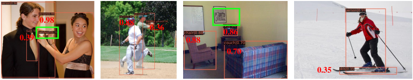
(a) Detection results of PVT [49]

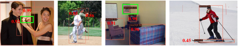
(b) Detection results of HLG

Figure 10: Qualitative object detection results on COCO 2017. The RetinaNet [93] is used as the framework with (a) PVT-Medium [49] and (b) HLG-Medium as the backbone in comparison.

(a) Segmentation results of PVT [49]

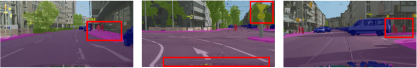
(b) Segmentation results of HLG

Figure 11: Qualitative semantic segmentation results on Cityscapes. The UperNet is used as the framework with (a) PVT-Medium [49] and (b) HLG-Medium as the backbone in comparison.

We further provide qualitative evaluation by visualizing the results of object detection and semantic segmentation. We compare our HLG-Medium and PVT-M with similar parameters. For object detection, we use RetinaNet as the framework on COCO. As shown in Figure 10, it is clear that HLG Transformer is superior in detecting small objects, thanks to its ability of better perceiving intra- and inter-patch in visual representation learning. For semantic segmentation, we use the UperNet as the framework on Cityscapes. It is shown in Figure 11 that our HLG Transformer can better segment small object instances. For example, in the first sample, HLG Transformer can infer the segmentation of pedestrians and railings more accurately. In the second sample, the traffic sign can be segmented better by HLG. In the last example, PVT cannot tell apart from the pedestrians and background around the boundary as well as HLG.

7 Conclusion

In this work, we have presented an alternative perspective for visual representation learning of dense visual prediction tasks by exploiting the ViT architectures. Instead of gradually increasing the receptive field with CNN models, we made a step change at the architectural level to elegantly solve the limited receptive field challenge. We implemented the proposed idea with Transformers capable of modeling global context at every stage of representation learning. For tackling general dense visual prediction tasks in a cost-effective manner, we further introduce Hierarchical Local Global (HLG) Transformers with local visual priors and global context learning integrated coherently in a unified architecture. Extensive experiments demonstrate that our models outperform existing alternatives on several visual recognition tasks.

8 Data Availability Statement

The datasets generated during and/or analysed during the current study are available in the Imagenet [79] (https://www.image-net.org/), ImageNet-v2 [90] (https://github.com/modestyachts/ImageNetV2), COCO [92] (https://cocodataset.org), ADE20K [62] (https://groups.csail.mit.edu/vision/datasets/ADE20K/), Cityscapes [97] (https://www.cityscapes-dataset.com), Pascal Context [63] (https://cs.stanford.edu/~roozbeh/pascal-context/) repositories.

Appendix A Visualizations

A.1 Position embedding

Visualization of the learned position embedding in Figure 12 shows that the model learns to encode distance within the image in the similarity of position embeddings.

A.2 Features

Figure 14 shows the feature visualization of our SETR-PUP. For the encoder, 24 output features from the 24 Transformer layers namely $Z^{1}-Z^{24}$ are collected. Meanwhile, 5 features ($U^{1}-U^{5}$) right after each bilinear interpolation in the decoder head are visited.

A.3 Attention maps

Attention maps (Figure 15) in each Transformer layer catch our interest. There are 16 heads and 24 layers in T-large. Similar to [98], a recursion perspective into this problem is applied. Figure 13 shows the attention maps of different selected spatial points (red).

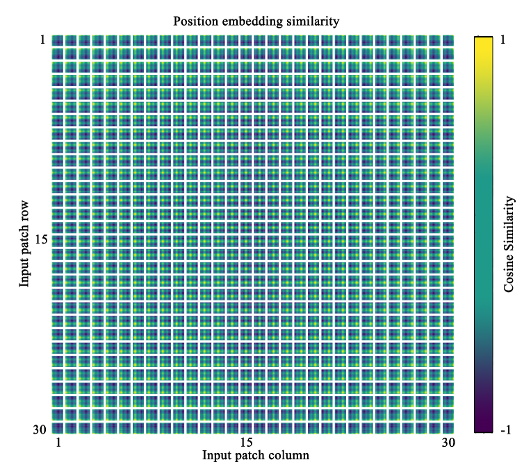
Figure 12: Similarity of position embeddings of SETR-PUP trained on Pascal Context. Tiles show the cosine similarity between the position embedding of the patch with the indicated row and column and the position embeddings of all other patches.

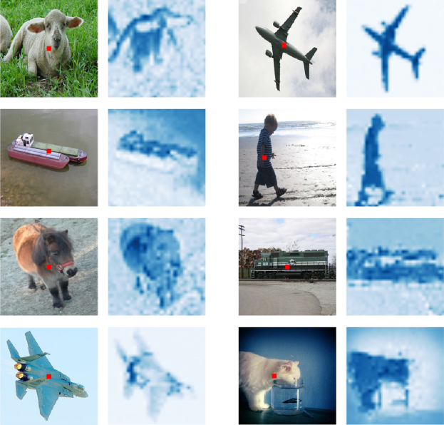
Figure 13: The first and third columns show images from Pascal Context. The second and fourth columns illustrate the attention map of the picked points (red).

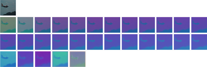
Figure 14: Visualization of output feature of layer $Z^{1}-Z^{24}$ and $U^{1}-U^{5}$ of SETR-PUP trained on Pascal Context. Best view in color. First row: The input image. Second row: Layer $Z^{1}$-$Z^{12}$. Third row: Layer $Z^{13}$-$Z^{24}$. Fourth row: Layer $U^{1}-U^{5}$.

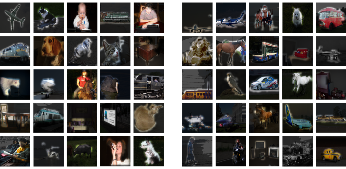
Figure 15: More examples of attention maps from SETR-PUP trained on Pascal Context.

References

- \bibcommenthead
- Dosovitskiy et al. [2021] Dosovitskiy, A., Beyer, L., Kolesnikov, A., Weissenborn, D., Zhai, X., Unterthiner, T., Dehghani, M., Minderer, M., Heigold, G., Gelly, S., et al.: An image is worth 16x16 words: Transformers for image recognition at scale. In: International Conference on Learning Representations (2021)
- Krizhevsky et al. [2012] Krizhevsky, A., Sutskever, I., Hinton, G.E.: ImageNet classification with deep convolutional neural networks. In: Advances in Neural Information Processing Systems (2012)
- Simonyan and Zisserman [2015] Simonyan, K., Zisserman, A.: Very deep convolutional networks for large-scale image recognition. In: International Conference on Learning Representations (2015)
- He et al. [2016] He, K., Zhang, X., Ren, S., Sun, J.: Deep residual learning for image recognition. In: IEEE Conference on Computer Vision and Pattern Recognition (2016)
- Szegedy et al. [2015] Szegedy, C., Liu, W., Jia, Y., Sermanet, P., Reed, S.E., Anguelov, D., Erhan, D., Vanhoucke, V., Rabinovich, A.: Going deeper with convolutions. In: IEEE Conference on Computer Vision and Pattern Recognition (2015)
- Huang et al. [2017] Huang, G., Liu, Z., Maaten, L., Weinberger, K.Q.: Densely connected convolutional networks. In: IEEE Conference on Computer Vision and Pattern Recognition (2017)
- Zheng et al. [2021] Zheng, S., Lu, J., Zhao, H., Zhu, X., Luo, Z., Wang, Y., Fu, Y., Feng, J., Xiang, T., Torr, P.H., Zhang, L.: Rethinking semantic segmentation from a sequence-to-sequence perspective with transformers. In: IEEE Conference on Computer Vision and Pattern Recognition (2021)
- Long et al. [2015] Long, J., Shelhamer, E., Darrell, T.: Fully convolutional networks for semantic segmentation. In: IEEE Conference on Computer Vision and Pattern Recognition (2015)
- Badrinarayanan et al. [2017] Badrinarayanan, V., Kendall, A., Cipolla, R.: Segnet: A deep convolutional encoder-decoder architecture for image segmentation. IEEE Transactions on Pattern Analysis and Machine Intelligence (2017)
- Yang et al. [2018] Yang, M., Yu, K., Zhang, C., Li, Z., Yang, K.: Denseaspp for semantic segmentation in street scenes. In: IEEE Conference on Computer Vision and Pattern Recognition (2018)
- Peng et al. [2017] Peng, C., Zhang, X., Yu, G., Luo, G., Sun, J.: Large kernel matters — improve semantic segmentation by global convolutional network. In: IEEE Conference on Computer Vision and Pattern Recognition (2017)
- Holschneider et al. [1990] Holschneider, M., Kronland-Martinet, R., Morlet, J., Tchamitchian, P.: A real-time algorithm for signal analysis with the help of the wavelet transform. In: Wavelets (1990)
- Chen et al. [2018] Chen, L.-C., Papandreou, G., Kokkinos, I., Murphy, K., Yuille, A.L.: Deeplab: Semantic image segmentation with deep convolutional nets, atrous convolution, and fully connected crfs. IEEE Transactions on Pattern Analysis and Machine Intelligence (2018)
- Zhao et al. [2017] Zhao, H., Shi, J., Qi, X., Wang, X., Jia, J.: Pyramid scene parsing network. In: IEEE Conference on Computer Vision and Pattern Recognition (2017)
- Wang et al. [2018] Wang, X., Girshick, R., Gupta, A., He, K.: Non-local neural networks. In: IEEE Conference on Computer Vision and Pattern Recognition (2018)
- Huang et al. [2019] Huang, Z., Wang, X., Huang, L., Huang, C., Wei, Y., Liu, W.: Ccnet: Criss-cross attention for semantic segmentation. In: IEEE International Conference on Computer Vision (2019)
- Li et al. [2019] Li, X., Zhang, L., You, A., Yang, M., Yang, K., Tong, Y.: Global aggregation then local distribution in fully convolutional networks. In: British Machine Vision Conference (2019)
- Wang et al. [2020] Wang, H., Zhu, Y., Green, B., Adam, H., Yuille, A., Chen, L.-C.: Axial-deeplab: Stand-alone axial-attention for panoptic segmentation. In: European Conference on Computer Vision (2020)
- Liu et al. [2021] Liu, Z., Lin, Y., Cao, Y., Hu, H., Wei, Y., Zhang, Z., Lin, S., Guo, B.: Swin transformer: Hierarchical vision transformer using shifted windows. In: IEEE International Conference on Computer Vision (2021)
- Wang et al. [2021] Wang, W., Xie, E., Li, X., Fan, D.-P., Song, K., Liang, D., Lu, T., Luo, P., Shao, L.: Pvtv2: Improved baselines with pyramid vision transformer. arXiv preprint (2021)
- Chen et al. [2022] Chen, C.-F., Panda, R., Fan, Q.: Regionvit: Regional-to-local attention for vision transformers. In: International Conference on Learning Representations (2022)
- Li et al. [2021] Li, Y., Zhang, K., Cao, J., Timofte, R., Van Gool, L.: Localvit: Bringing locality to vision transformers. arXiv preprint (2021)
- d’Ascoli et al. [2021] d’Ascoli, S., Touvron, H., Leavitt, M.L., Morcos, A.S., Biroli, G., Sagun, L.: Convit: Improving vision transformers with soft convolutional inductive biases. In: International Conference on Machine Learning (2021)
- Chu et al. [2021] Chu, X., Tian, Z., Wang, Y., Zhang, B., Ren, H., Wei, X., Xia, H., Shen, C.: Twins: Revisiting the design of spatial attention in vision transformers. In: Advances in Neural Information Processing Systems (2021)
- Chen et al. [2015] Chen, L., Papandreou, G., Kokkinos, I., Murphy, K., Yuille, A.L.: Semantic image segmentation with deep convolutional nets and fully connected CRFs. In: International Conference on Learning Representations (2015)
- Liu et al. [2015] Liu, Z., Li, X., Luo, P., Loy, C.C., Tang, X.: Semantic image segmentation via deep parsing network. In: IEEE International Conference on Computer Vision (2015)
- Zheng et al. [2015] Zheng, S., Jayasumana, S., Romera-Paredes, B., Vineet, V., Su, Z., Du, D., Huang, C., Torr, P.H.S.: Conditional random fields as recurrent neural networks. In: IEEE International Conference on Computer Vision (2015)
- Ronneberger et al. [2015] Ronneberger, O., Fischer, P., Brox, T.: U-net: Convolutional networks for biomedical image segmentation. International Conference on Medical Image Computing and Computer Assisted Intervention (2015)
- Noh et al. [2015] Noh, H., Hong, S., Han, B.: Learning deconvolution network for semantic segmentation. In: IEEE International Conference on Computer Vision (2015)
- Chen et al. [2015] Chen, L.-C., Papandreou, G., Kokkinos, I., Murphy, K., Yuille, A.L.: Semantic image segmentation with deep convolutional nets and fully connected CRFs. In: International Conference on Learning Representations (2015)
- Yu and Koltun [2016] Yu, F., Koltun, V.: Multi-scale context aggregation by dilated convolutions. International Conference on Learning Representations (2016)
- Chen et al. [2018] Chen, L.-C., Papandreou, G., Kokkinos, I., Murphy, K., Yuille, A.L.: Deeplab: Semantic image segmentation with deep convolutional nets, atrous convolution, and fully connected crfs. IEEE Transactions on Pattern Analysis and Machine Intelligence (2018)
- Zhao et al. [2018] Zhao, H., Zhang, Y., Liu, S., Shi, J., Change Loy, C., Lin, D., Jia, J.: Psanet: Point-wise spatial attention network for scene parsing. In: European Conference on Computer Vision (2018)
- Fu et al. [2019] Fu, J., Liu, J., Tian, H., Fang, Z., Lu, H.: Dual attention network for scene segmentation. In: IEEE Conference on Computer Vision and Pattern Recognition (2019)
- Huang et al. [2019] Huang, Z., Wang, X., Huang, L., Huang, C., Wei, Y., Liu, W.: Ccnet: Criss-cross attention for semantic segmentation. In: IEEE International Conference on Computer Vision (2019)
- Zhang et al. [2020] Zhang, L., Xu, D., Arnab, A., Torr, P.H.: Dynamic graph message passing networks. In: IEEE Conference on Computer Vision and Pattern Recognition (2020)
- Vaswani et al. [2017] Vaswani, A., Shazeer, N., Parmar, N., Uszkoreit, J., Jones, L., Gomez, A.N., Kaiser, Ł., Polosukhin, I.: Attention is all you need. In: Advances in Neural Information Processing Systems (2017)
- Devlin et al. [2019] Devlin, J., Chang, M.-W., Lee, K., Toutanova, K.: BERT: Pre-training of deep bidirectional transformers for language understanding. In: NAACL-HLT (2019)
- Dai et al. [2019] Dai, Z., Yang, Z., Yang, Y., Carbonell, J., Le, Q.V., Salakhutdinov, R.: Transformer-XL: Attentive language models beyond a fixed-length context. In: ACL (2019)
- Yang et al. [2019] Yang, Z., Dai, Z., Yang, Y., Carbonell, J., Salakhutdinov, R., Le, Q.V.: XLNet: Generalized autoregressive pretraining for language understanding. In: Advances in Neural Information Processing Systems (2019)
- Bello et al. [2019] Bello, I., Zoph, B., Vaswani, A., Shlens, J., Le, Q.V.: Attention augmented convolutional networks. In: IEEE International Conference on Computer Vision (2019)
- Hu et al. [2019] Hu, H., Zhang, Z., Xie, Z., Lin, S.: Local relation networks for image recognition. In: IEEE International Conference on Computer Vision (2019)
- Ramachandran et al. [2019] Ramachandran, P., Parmar, N., Vaswani, A., Bello, I., Levskaya, A., Shlens, J.: Stand-alone self-attention in vision models. In: Advances in Neural Information Processing Systems (2019)
- Zhao et al. [2020] Zhao, H., Jia, J., Koltun, V.: Exploring self-attention for image recognition. In: IEEE Conference on Computer Vision and Pattern Recognition (2020)
- Carion et al. [2020] Carion, N., Massa, F., Synnaeve, G., Usunier, N., Kirillov, A., Zagoruyko, S.: End-to-end object detection with transformers. In: European Conference on Computer Vision (2020)
- Li et al. [2020] Li, Z., Liu, X., Creighton, F.X., Taylor, R.H., Unberath, M.: Revisiting stereo depth estimation from a sequence-to-sequence perspective with transformers. arXiv preprint (2020)
- Liu et al. [2020] Liu, R., Yuan, Z., Liu, T., Xiong, Z.: End-to-end lane shape prediction with transformers. In: IEEE Winter Conference on Applications of Computer Vision (2020)
- Ho et al. [2019] Ho, J., Kalchbrenner, N., Weissenborn, D., Salimans, T.: Axial attention in multidimensional transformers. arXiv preprint (2019)
- Wang et al. [2021] Wang, W., Xie, E., Li, X., Fan, D.-P., Song, K., Liang, D., Lu, T., Luo, P., Shao, L.: Pyramid vision transformer: A versatile backbone for dense prediction without convolutions. In: IEEE International Conference on Computer Vision (2021)
- Wu et al. [2021] Wu, H., Xiao, B., Codella, N., Liu, M., Dai, X., Yuan, L., Zhang, L.: Cvt: Introducing convolutions to vision transformers. In: IEEE International Conference on Computer Vision (2021)
- Chen et al. [2021] Chen, C.-F.R., Fan, Q., Panda, R.: Crossvit: Cross-attention multi-scale vision transformer for image classification. In: IEEE International Conference on Computer Vision (2021)
- Zhang et al. [2019] Zhang, L., Li, X., Arnab, A., Yang, K., Tong, Y., Torr, P.H.: Dual graph convolutional network for semantic segmentation. In: British Machine Vision Conference (2019)
- Veličković et al. [2018] Veličković, P., Cucurull, G., Casanova, A., Romero, A., Lio, P., Bengio, Y.: Graph attention networks. In: International Conference on Learning Representations (2018)
- Lin et al. [2017] Lin, T.-Y., Dollár, P., Girshick, R.B., He, K., Hariharan, B., Belongie, S.J.: Feature pyramid networks for object detection. In: IEEE Conference on Computer Vision and Pattern Recognition (2017)
- Kirillov et al. [2019] Kirillov, A., Girshick, R., He, K., Dollár, P.: Panoptic feature pyramid networks. In: IEEE Conference on Computer Vision and Pattern Recognition (2019)
- Chollet [2017] Chollet, F.: Xception: Deep learning with depthwise separable convolutions. In: IEEE Conference on Computer Vision and Pattern Recognition (2017)
- Sandler et al. [2018] Sandler, M., Howard, A., Zhu, M., Zhmoginov, A., Chen, L.-C.: Mobilenetv2: Inverted residuals and linear bottlenecks. In: IEEE Conference on Computer Vision and Pattern Recognition (2018)
- Yang et al. [2022] Yang, C., Qiao, S., Yu, Q., Yuan, X., Zhu, Y., Yuille, A., Adam, H., Chen, L.-C.: Moat: Alternating mobile convolution and attention brings strong vision models. arXiv preprint (2022)
- Hu et al. [2018] Hu, J., Shen, L., Sun, G.: Squeeze-and-excitation networks. In: IEEE Conference on Computer Vision and Pattern Recognition (2018)
- OpenMMLab [2020] OpenMMLab: mmsegmentation. https://github.com/open-mmlab/mmsegmentation (2020)
- Cordts et al. [2016] Cordts, M., Omran, M., Ramos, S., Rehfeld, T., Enzweiler, M., Benenson, R., Franke, U., Roth, S., Schiele, B.: The cityscapes dataset for semantic urban scene understanding. In: IEEE Conference on Computer Vision and Pattern Recognition (2016)
- Zhou et al. [2016] Zhou, B., Zhao, H., Puig, X., Fidler, S., Barriuso, A., Torralba, A.: Semantic understanding of scenes through the ade20k dataset. arXiv preprint (2016)
- Mottaghi et al. [2014] Mottaghi, R., Chen, X., Liu, X., Cho, N.-G., Lee, S.-W., Fidler, S., Urtasun, R., Yuille, A.: The role of context for object detection and semantic segmentation in the wild. In: IEEE Conference on Computer Vision and Pattern Recognition (2014)
- Hou et al. [2020] Hou, Q., Zhang, L., Cheng, M.-M., Feng, J.: Strip pooling: Rethinking spatial pooling for scene parsing. In: IEEE Conference on Computer Vision and Pattern Recognition (2020)
- Yuan et al. [2020] Yuan, Y., Chen, X., Wang, J.: Object-contextual representations for semantic segmentation. In: European Conference on Computer Vision (2020)
- Xiao et al. [2018] Xiao, T., Liu, Y., Zhou, B., Jiang, Y., Sun, J.: Unified perceptual parsing for scene understanding. In: European Conference on Computer Vision (2018)
- Chen et al. [2018] Chen, L.-C., Zhu, Y., Papandreou, G., Schroff, F., Adam, H.: Encoder-decoder with atrous separable convolution for semantic image segmentation. In: European Conference on Computer Vision (2018)
- Yuan and Wang [2018] Yuan, Y., Wang, J.: Ocnet: Object context network for scene parsing. arXiv preprint (2018)
- Li et al. [2019] Li, X., Zhong, Z., Wu, J., Yang, Y., Lin, Z., Liu, H.: Expectation-maximization attention networks for semantic segmentation. In: IEEE Conference on Computer Vision and Pattern Recognition (2019)
- Ding et al. [2019] Ding, H., Jiang, X., Shuai, B., Liu, A.Q., Wang, G.: Semantic correlation promoted shape-variant context for segmentation. In: IEEE Conference on Computer Vision and Pattern Recognition (2019)
- Li et al. [2020] Li, X., Zhao, H., Han, L., Tong, Y., Yang, K.: Gff: Gated fully fusion for semantic segmentation. In: AAAI Conference on Artificial Intelligence (2020)
- He et al. [2019] He, J., Deng, Z., Zhou, L., Wang, Y., Qiao, Y.: Adaptive pyramid context network for semantic segmentation. In: IEEE Conference on Computer Vision and Pattern Recognition (2019)
- Touvron et al. [2020] Touvron, H., Cord, M., Douze, M., Massa, F., Sablayrolles, A., Jégou, H.: Training data-efficient image transformers & distillation through attention. arXiv preprint (2020)
- Bao et al. [2022] Bao, H., Dong, L., Piao, S., Wei, F.: Beit: Bert pre-training of image transformers. In: International Conference on Learning Representations (2022)
- Chen et al. [2017] Chen, L.-C., Papandreou, G., Schroff, F., Adam, H.: Rethinking atrous convolution for semantic image segmentation. arXiv preprint (2017)
- Cao et al. [2019] Cao, Y., Xu, J., Lin, S., Wei, F., Hu, H.: Gcnet: Non-local networks meet squeeze-excitation networks and beyond. In: IEEE International Conference on Computer Vision Workshops (2019)
- Yu et al. [2018] Yu, C., Wang, J., Peng, C., Gao, C., Yu, G., Sang, N.: Bisenet: Bilateral segmentation network for real-time semantic segmentation. In: European Conference on Computer Vision (2018)
- Cheng et al. [2020] Cheng, B., Collins, M.D., Zhu, Y., Liu, T., Huang, T.S., Adam, H., Chen, L.-C.: Panoptic-deeplab: A simple, strong, and fast baseline for bottom-up panoptic segmentation. In: IEEE Conference on Computer Vision and Pattern Recognition (2020)
- Russakovsky et al. [2015] Russakovsky, O., Deng, J., Su, H., Krause, J., Satheesh, S., Ma, S., Huang, Z., Karpathy, A., Khosla, A., Bernstein, M., Berg, A.C., Fei-Fei, L.: Imagenet large scale visual recognition challenge. International Journal of Computer Vision (2015)
- Zhang et al. [2017] Zhang, H., Cisse, M., Dauphin, Y.N., Lopez-Paz, D.: mixup: Beyond empirical risk minimization. arXiv preprint arXiv:1710.09412 (2017)
- Larsson et al. [2016] Larsson, G., Maire, M., Shakhnarovich, G.: Fractalnet: Ultra-deep neural networks without residuals. arXiv preprint arXiv:1605.07648 (2016)
- Heo et al. [2021] Heo, B., Yun, S., Han, D., Chun, S., Choe, J., Oh, S.J.: Rethinking spatial dimensions of vision transformers. In: IEEE International Conference on Computer Vision (2021)
- Yan et al. [2021] Yan, H., Li, Z., Li, W., Wang, C., Wu, M., Zhang, C.: Contnet: Why not use convolution and transformer at the same time? arXiv preprint (2021)
- Bai et al. [2021] Bai, S., Torr, P., et al.: Visual parser: Representing part-whole hierarchies with transformers. arXiv preprint (2021)
- Zhang et al. [2021] Zhang, Z., Zhang, H., Zhao, L., Chen, T., Pfister, T.: Aggregating nested transformers. arXiv preprint (2021)
- Dai et al. [2021] Dai, Z., Liu, H., Le, Q.V., Tan, M.: Coatnet: Marrying convolution and attention for all data sizes. In: Advances in Neural Information Processing Systems (2021)
- Touvron et al. [2022] Touvron, H., Cord, M., Jégou, H.: Deit iii: Revenge of the vit. In: Computer Vision–ECCV 2022: 17th European Conference, Tel Aviv, Israel, October 23–27, 2022, Proceedings, Part XXIV, pp. 516–533 (2022). Springer
- Liu et al. [2022a] Liu, Z., Hu, H., Lin, Y., Yao, Z., Xie, Z., Wei, Y., Ning, J., Cao, Y., Zhang, Z., Dong, L., et al.: Swin transformer v2: Scaling up capacity and resolution. In: IEEE Conference on Computer Vision and Pattern Recognition (2022)
- Liu et al. [2022b] Liu, Z., Mao, H., Wu, C.-Y., Feichtenhofer, C., Darrell, T., Xie, S.: A convnet for the 2020s. In: IEEE Conference on Computer Vision and Pattern Recognition (2022)
- Recht et al. [2019] Recht, B., Roelofs, R., Schmidt, L., Shankar, V.: Do imagenet classifiers generalize to imagenet? In: International Conference on Machine Learning (2019)
- Long et al. [2015] Long, J., Shelhamer, E., Darrell, T.: Fully convolutional networks for semantic segmentation. In: IEEE Conference on Computer Vision and Pattern Recognition (2015)
- Lin et al. [2014] Lin, T.-Y., Maire, M., Belongie, S., Hays, J., Perona, P., Ramanan, D., Dollár, P., Zitnick, C.L.: Microsoft coco: Common objects in context. In: European Conference on Computer Vision (2014)
- Lin et al. [2017] Lin, T.-Y., Goyal, P., Girshick, R., He, K., Dollar, P.: Focal loss for dense object detection. In: IEEE International Conference on Computer Vision (2017)
- He et al. [2017] He, K., Gkioxari, G., Dollár, P., Girshick, R.: Mask r-cnn. In: IEEE International Conference on Computer Vision (2017)
- Zhang et al. [2021] Zhang, P., Dai, X., Yang, J., Xiao, B., Yuan, L., Zhang, L., Gao, J.: Multi-scale vision longformer: A new vision transformer for high-resolution image encoding. In: IEEE International Conference on Computer Vision (2021)
- Xie et al. [2017] Xie, S., Girshick, R., Dollár, P., Tu, Z., He, K.: Aggregated residual transformations for deep neural networks. In: IEEE Conference on Computer Vision and Pattern Recognition (2017)
- Cordts et al. [2016] Cordts, M., Omran, M., Ramos, S., Rehfeld, T., Enzweiler, M., Benenson, R., Franke, U., Roth, S., Schiele, B.: The cityscapes dataset for semantic urban scene understanding. In: IEEE Conference on Computer Vision and Pattern Recognition (2016)
- Abnar and Zuidema [2020] Abnar, S., Zuidema, W.: Quantifying attention flow in transformers. arXiv preprint (2020)