Probabilistic Reconciliation of Count Time Series

Abstract

Forecast reconciliation is an important research topic. Yet, there is currently neither formal framework nor practical method for the probabilistic reconciliation of count time series. In this paper we propose a definition of coherency and reconciled probabilistic forecast which applies to both real-valued and count variables and a novel method for probabilistic reconciliation. It is based on a generalization of Bayes’ rule and it can reconcile both real-value and count variables. When applied to count variables, it yields a reconciled probability mass function. Our experiments with the temporal reconciliation of count variables show a major forecast improvement compared to the probabilistic Gaussian reconciliation.

1 Introduction

Time series are often organized into a hierarchy. For example, the total sales of a product in a country can be divided into regions and then into sub-regions. Forecasts of hierarchical time series should be coherent; for instance, the sum of the forecasts of the different regions should be equal to the forecast for the entire country. Forecasts are incoherent if they do not satisfy such constraints. Reconciliation methods [13, 31] compute coherent forecasts by combining the base forecasts generated independently for each time series, possibly incorporating non-negativity constraints [32]. Reconciled forecasts are generally more accurate than the base forecasts; indeed, forecast reconciliation is related to forecast combination [9, 6].

A special case of reconciliation is constituted by temporal hierarchies [1], which reconcile base forecasts computed for the same variable at different frequencies (e.g., monthly, quarterly and yearly); they generally improve the forecasts [19] of smooth and intermittent time series.

As for probabilistic reconciliation, [25] proposed a seminal framework which interprets reconciliation as a projection. Other methods for probabilistic reconciliation have been proposed [15, 4, 30, 27], but none of them reconciles count variables.

Our first contribution is the definition of coherency and reconciliation for count variables. Then, we propose a novel approach for probabilistic reconciliation, based on conditioning. As a first step, our method computes a joint distribution on the entire hierarchy, using as source of information the base forecast of the bottom variables; this is the probabilistic bottom-up reconciliation. Then it updates the joint distribution by conditioning on the information contained in the base forecast of the upper variables, using the method of virtual evidence [26, 3]. Our approach can reconcile both real-value and count variables; in this paper however we focus on count variables. In this case, we obtain a reconciled probability mass function defined over counts. We show extensive experiments on the temporal reconciliation of count time series, reporting major empirical improvements compared to probabilistic reconciliation based on Gaussian assumptions.

The paper is organized as follows: Section 2 reviews temporal hierarchies; in Section 3 we propose a definition of coherent and reconciled forecasts which applies to both continuous and real-valued variables. In Section 4 we describe our reconciliation method and in Section 5 we present the experimental results.

2 Temporal Hierarchies

Temporal hierarchies [1] enforce coherence between forecasts generated at different temporal scales. For instance the temporal hierarchy of Figure 1 is built on top of a quarterly time series observed over $t$ years, with observations $q_{1},\ldots,q_{4},q_{5},\ldots,q_{4\cdot t}$. The bottom level of the hierarchy contains quarterly observations grouped in vectors $\mathcal{Q}_{j}=[q_{k}:k\mod 4=j]$, $j=1,\ldots,4$; the semi-annual observations are grouped in the vectors $\mathcal{S}_{j}=[s_{\ell}:\ell\mod 2=j]$ where $s_{2i-1}=q_{4(i-1)+1}+q_{4(i-1)+2}$, $s_{2i}=q_{4(i-1)+3}+q_{4i}$ for $i=1,\ldots,t$; finally the annual observations are grouped as $\mathcal{Y}=[a_{1},\ldots,a_{t}]$, where $a_{i}=s_{2i-1}+s_{2i}$, for $i=1,\ldots,t$.

Figure 1: Temporal hierarchy built on top of a quarterly time series.

We denote by $\mathbf{b}$ the vector of bottom observations, e.g., $\mathbf{b}=[\mathcal{Q}_{1}^{T},\mathcal{Q}_{2}^{T},\mathcal{Q}_{3}^{T},\mathcal{Q}_{4}^{T}]^{T}$, and by $\mathbf{u}$ the vector of upper observations, e.g., $\mathbf{u}=[\mathcal{Y}^{T},\mathcal{S}_{1}^{T},\mathcal{S}_{2}^{T}]^{T}$. We denote by $\mathbf{y}$ the vector containing all the observations of the temporal hierarchy, e.g., $\mathbf{y}=[\mathbf{u}\ \mathbf{b}]=[\mathcal{Y}^{T},\mathcal{S}_{1}^{T},\mathcal{S}_{2}^{T},\mathcal{Q}_{1}^{T},\mathcal{Q}_{2}^{T},\mathcal{Q}_{3}^{T},\mathcal{Q}_{4}^{T}]^{T}$. We denote by $m$ the number of bottom observations and by $n$ the total number of observations in the hierarchy.

A hierarchy is characterized by its summing matrix $\mathbf{S}\in\mathbb{R}^{n\times m}$ that defines the relationship between $\mathbf{b}$ and $\mathbf{y}$, i.e.

$$\mathbf{y}=\mathbf{S}\mathbf{b}.$$

The $\mathbf{S}$ matrix of hierarchy in Figure 1 is:

$$\mathbf{S}=\begin{bmatrix}1&\,\,\,&1&\,\,\,&1&\,\,\,&1\\ 1&\,\,\,&1&\,\,\,&0&\,\,\,&0\\ 0&\,\,\,&0&\,\,\,&1&\,\,\,&1\\ 1&\,\,\,&0&\,\,\,&0&\,\,\,&0\\ 0&\,\,\,&1&\,\,\,&0&\,\,\,&0\\ 0&\,\,\,&0&\,\,\,&1&\,\,\,&0\\ 0&\,\,\,&0&\,\,\,&0&\,\,\,&1\\ \end{bmatrix}=\begin{bmatrix}&\,\,\,&&\,\,\,&&\,\,\,&\\ &\,\,\,&&\makebox(0.0,0.0)[]{\text{\huge{A}}}&&\,\,\,&\\ &\,\,\,&&\,\,\,&\,\,\,&&\\ \cdashline{2-6}\ &\,\,\,&&\,\,\,&&\,\,\,&\\ &\,\,\,&&\makebox(0.0,0.0)[]{\text{\huge{I}}}&&\,\,\,&\\ &\,\,\,&&\,\,\,&&\,\,\,&\\ &\,\,\,&&\,\,\,&&\,\,\,&\end{bmatrix},$$

where $\mathbf{A}\in\mathbb{R}^{(n-m)\times m}$ encodes which bottom time series should be summed up in order to obtain each upper time series.

Reconciling temporal hierarchies

Let us denote by $h$ the forecast horizon, expressed in years. For instance, $h$=1 implies four forecasts at the quarterly level, two forecasts at the bi-annual level and one forecast at the yearly level.

Let us denote by $\hat{\mathbf{u}}_{h}$ and $\hat{\mathbf{b}}_{h}$ the base point forecasts for the upper and bottom levels of the hierarchy. The vector of the base point forecasts for the entire hierarchy is $\hat{\mathbf{y}}_{h}=\begin{bmatrix}\hat{\mathbf{u}}_{h}\\ \hat{\mathbf{b}}_{h}\end{bmatrix}$,

The base forecast are incoherent, i.e., $\hat{\mathbf{y}}_{h}\neq\mathbf{S}\hat{\mathbf{b}}_{h}$. Optimal reconciliation methods [13, 31] adjust the forecast for the bottom level and sum them up in order to obtain the forecast for the upper levels. The reconciled forecasts of the bottom time series and the entire hierarchy are:

$$\tilde{\mathbf{b}}_{h} =\mathbf{G}\hat{\mathbf{y}}_{h}$$ (1)

$$\tilde{\mathbf{y}}_{h} =\mathbf{S}\tilde{\mathbf{b}}_{h}=\mathbf{SG}\hat{\mathbf{y}}_{h}.$$ (2)

The core of the minT algorithm [31] is the following expression for $\mathbf{G}$, which minimizes the mean squared error of the coherent forecast:

$$\mathbf{G}=(\mathbf{S}^{T}\mathbf{W}^{-1}\mathbf{S})^{-1}\mathbf{S}^{T}\mathbf{W}^{-1}\,,$$ (3)

where $\mathbf{W}$ is the covariance matrix of the errors of the base forecast. The covariance of the reconciled forecasts is [31]

$$\operatorname{Var}(\tilde{\mathbf{y}})=\mathbf{S}\mathbf{G}\mathbf{W}\mathbf{G}^{T}\mathbf{S}^{T}=\mathbf{S}(\mathbf{S}^{T}\mathbf{W}^{-1}\mathbf{S})^{-1}\mathbf{S}^{T}\,.$$ (4)

In temporal hierarchies, $\mathbf{W}$ is generally assumed to be diagonal, but it can be defined in different ways. For instance, hierarchy variance [1] adopts the same variances of the base forecasts, allowing heterogeneity within each level of the hierarchy. For the hierarchy of Fig.1 it yields:

$$\mathbf{W}=\text{diag}(\hat{\sigma}_{Y}^{2},\hat{\sigma}_{S_{1}}^{2},\hat{\sigma}_{S_{2}}^{2},\hat{\sigma}_{Q_{1}}^{2},\ldots,\hat{\sigma}_{Q_{4}}^{2})\,.$$

Instead, structural scaling [1] defines $\mathbf{W}$ by assuming: i) the forecasts of the same level to have the same variance; ii) the variance at each level to be proportional to the number of bottom time series that are summed up in that level. For the hierarchy of Fig.1, it yields:

$$\mathbf{W}=\text{diag}(4,2,1,1,1,1)\,.$$

3 Probabilistic Reconciliation

The methods discussed so far reconcile the point forecasts. In the following we review the most important methods for probabilistic reconciliation.

Jeon et al. [15] propose different heuristics (based on minT) for probabilistic reconciliation, one of which is equivalent to reconciling a large number of forecast quantiles. The algorithm by [30] yields coherent probabilistic forecasts whose expected value match the mean of MinT; yet this method does not consider the variance of the base forecast of the upper variables. [27] propose a deep neural network model which produces coherent probabilistic forecasts without any post-processing step, by incorporating reconciliation within a single trainable model.

[4] shows that probabilistic reconciliation can be accomplished via Bayes’ rule. First they create a joint predictive distribution for the entire hierarchy, based on the probabilistic base forecast of the bottom time series. The distribution is then updated in order to accommodate the information contained in the base forecast of the upper time series. Under the Gaussian assumption they obtain the reconciled Gaussian distribution in closed form. The reconciled mean and variance are equivalent to those of minT, despite the different derivation strategy. Also [10] propose a Bayesian viewpoint of the reconciliation process.

Panagiotelis et al. [25] proposes a definition of probabilistic reconciliation based on projection and an algorithm which obtains the reconciled distribution by minimizing a scoring rule. However this requires optimizing via stochastic gradient descent the $m\times n$ elements of $\mathbf{G}$, which structurally limits its scalability.

There is currently no method for the reconciliation of count variables. To address this problem, we first extend to count variables the key definitions of Panagiotelis et al. [25].

3.1 Coherence and reconciliation according to [25]

Recalling that $m$ and $n$ denote the number of bottom and total time series, matrix $\mathbf{S}$ can be seen as a function $s:\mathbb{R}^{m}\rightarrow\mathbb{R}^{n}$ which associates to a bottom vector $\mathbf{b}\in\mathbb{R}^{m}$ the coherent vector $s(\mathbf{b})=\mathbf{S}\mathbf{b}\in\mathbb{R}^{n}$. The $n$-dimensional coherent vectors lie in the vector subspace $\mathfrak{s}$ (spanned by the columns of $\mathbf{S}$), which is well-defined in $\mathbb{R}^{n}$. The base forecasts of the bottom time series can be represented by a probability triple $(\mathbb{R}^{m},\mathcal{F}_{\mathbb{R}^{m}},\nu)$, where $\mathcal{F}_{\mathbb{R}^{m}}$ is the (Borel) $\sigma$-algebra associated with $\mathbb{R}^{m}$.

Definition 1.

[25] A probability triple $(\mathfrak{s},\mathcal{F}_{\mathfrak{s}},\check{\nu}_{\mathfrak{s}})$ is coherent with the bottom probability triple $(\mathbb{R}^{m},\mathcal{F}_{\mathbb{R}^{m}},\nu)$ if:

$$\check{\nu}_{\mathfrak{s}}(s(\mathcal{B}))=\nu(\mathcal{B}),\quad\forall\mathcal{B}\in\mathcal{F}_{\mathbb{R}^{m}},$$ (5)

Definition 5 implies that incoherent vectors have zero probability under the probability measure $\check{\nu}_{\mathfrak{s}}$.

3.2 Extension to count variables

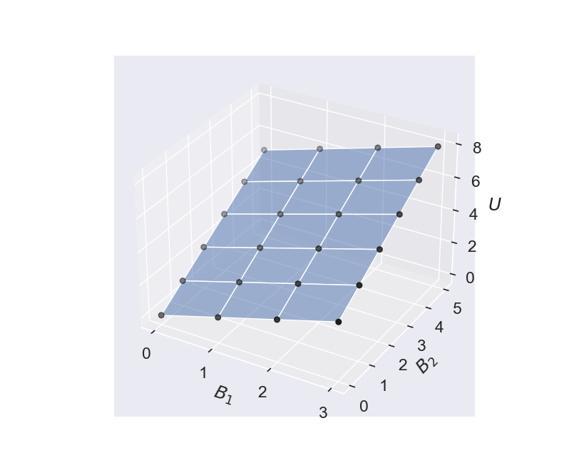
Figure 2: $B_{1}$ and $B_{2}$ are two count variables, with $U=B_{1}+B_{2}$. The black points constitute the set of coherent vectors.

A count variable takes non-negative integer values $\mathbb{N}=\{0,1,2,3,...\}$. We denote by $\mathbf{a}\in\mathbb{N}^{k}$ an array of $k$ non-negative integers which we call vectors, with a slight abuse of notation. We have vectors $\mathbf{y}\in\mathbb{N}^{n}$, $\mathbf{b}\in\mathbb{N}^{m}$ and $\mathbf{u}\in\mathbb{N}^{n-m}$. The set of coherent vectors in $\mathbb{N}^{n}$ is:

$$s(\mathbb{N}^{m})=\{\mathbf{y}\in\mathbb{N}^{n}:\exists\mathbf{b}\in\mathbb{N}^{m}\text{ such that }\mathbf{y}=s(\mathbf{b})\}.$$ (6)

Eq. (6) defines the subset of coherent vectors, see Fig.2 for a graphical representation. Indeed, no vector subspace can be defined with count variables. We can now extend to counts the definition of coherence:

Definition 2.

A probability triple $(s(\mathcal{X}^{m}),\mathcal{F}_{s(\mathcal{X}^{m})},\check{\nu})$ is coherent with the bottom probability triple $(\mathcal{X}^{m},\mathcal{F}_{\mathcal{X}^{m}},\nu)$ if:

$$\check{\nu}(s(\mathcal{B}))=\nu(\mathcal{B}),\quad\forall\mathcal{B}\in\mathcal{F}_{\mathcal{X}^{m}},$$ (7)

where $\mathcal{X}^{m}=\mathbb{R}^{m}$ in the continuous case and $\mathcal{X}^{m}=\mathbb{N}^{m}$ in the discrete case.

Definitions 5 and 2 are equivalent in the continuous case, as we prove in B. However, definition 2 applies also to count variables, in which case $\check{\nu}$ and $\nu$ are discrete probability distributions. Denoting by $\check{p}$ and $p$ their probability mass functions, we can write Eq. (7) as:

$$\check{p}(b_{1},\ldots,b_{m},\mathbf{u}=\mathbf{A}\mathbf{b})=p(b_{1},\ldots,b_{m}),\qquad\text{ for all }b_{1},\ldots,b_{m}\in\mathbb{N}$$ (8)

Equation (8) assigns zero probability to vectors of counts which are incoherent.

Definition 3.

Consider a probabilistic base forecast for $\mathbf{y}$, constituted by the probability triple $(\mathcal{X}^{n},\mathcal{F}_{\mathcal{X}^{n}},\hat{\nu})$. A reconciled probability distribution $\tilde{\nu}$ is a transformation of the forecast probability measure $\hat{\nu}$ which is coherent and defined on $\mathcal{F}_{s(\mathcal{X}^{m})}$.

Our definition of reconciled probability triple is more general than that of  Panagiotelis et al. [25], which requires a reconciliation function, defined in their algorithm as an affine map. This can lead to negatively reconciled forecasts, which is not admissible with count variables.

4 Reconciliation based on virtual evidence

We assume the forecasts over counts to be constituted by probability mass functions (pmfs). We denote by $\hat{p}$ and $p_{BU}$ the pmf of the base forecasts and the probabilistic bottom-up respectively. The reconciled pmf is denoted by $\tilde{p}$.

The first step of our algorithm is to create a joint pmf for the entire hierarchy using $\hat{p}(\mathbf{b})$ as the only source of information; this is the probabilistic bottom-up. In order to formalize it, we need an indicator function which selects the suitable vectors $\mathbf{u}$:

$$\mathds{1}_{\mathbf{A}\mathbf{b}}(\mathbf{u})=\begin{cases}1&\text{if }\mathbf{u}=\mathbf{A}\mathbf{b}\\ 0&\text{otherwise}\end{cases}.$$

The pmf $p_{BU}(\mathbf{y})$ is:

$$p_{BU}(\mathbf{y})=p_{BU}(\mathbf{u},\mathbf{b})=\ \mathds{1}_{\mathbf{A}\mathbf{b}}(\mathbf{u})\hat{p}(\mathbf{b}).$$

The pmf $p_{BU}(\mathbf{y})$ assigns positive probability only to vectors $\mathbf{y}\in s(\mathcal{X}^{m})$ because of the indicator $\mathds{1}_{\mathbf{A}\mathbf{b}}(\mathbf{u})$; it is thus coherent.

4.1 Conditioning on uncertain evidence

Virtual evidence [26] is a method for conditioning a joint distribution on an uncertain evidence, obtained for instance from a noisy source of information. It is also referred to as soft evidence “nothing else considered” by [5, 3.9] and [3].

Consider two discrete variables $X$ and $Z$ and their joint prior pmf $p(x,z)=p(x)p(z|x)$, where the values of $\{z\in z_{k}\}_{k=1}^{K}$ are mutually exclusive. Virtual evidence assumes that $\zeta$, i.e. the uncertain observation of $Z$, can be expressed by the likelihood ratios: $\lambda_{1}:...:\lambda_{K}=L(Z=z_{1}):...:L(Z=z_{K})$. Assuming $\zeta$ to be independent from the prior, the update rule (see Chan and Darwiche [3, Theorem 2] and Munk et al. [22]) is:

$$p(x|\zeta)=\frac{\sum_{k=1}^{K}p(x,z_{k})\lambda_{k}}{\sum_{j=1z}^{K}p(z_{j})\lambda_{j}}.$$ (9)

We can make a few observation about the update of Eq.(9). First, $p(x)$ and $p(x|\zeta)$ have the same zero probabilities. Indeed, virtual evidence is based on conditioning, which does not modify the zero probabilities [5, Chapter 3.3].

If there is a unique $\lambda_{j}$>0 and the remaining $\lambda_{i}$ ($i\neq j$) are zero, we have a certain observation ($Z=z_{j}$). In this case, the conditioning of Eq.(9) is equivalent to Bayes’ rule.

The evidence $\zeta$ does not need to be normalized, as what matters are the likelihood ratios. However in our application $\zeta$ is constituted by the base forecast of the upper variables and thus it is normalized.

4.2 Reconciliation by conditioning on the base forecast of the upper time series

We now show how to use virtual evidence in order to condition $p_{BU}(\mathbf{u},\mathbf{b})$ on the base forecasts $\hat{p}(u_{1})$ of the first upper time series $u_{1}$. Let us denote by $\mathbf{A}_{[1,]}$ the first row of $\mathbf{A}$, such that $u_{1}=\mathbf{A}_{[1,]}\mathbf{b}$. According to Eq.(9), the reconciled pmf of the bottom time series is:

$$\tilde{p}_{1}(\mathbf{b})=\dfrac{\sum_{u_{1}^{*}}p_{BU}(u_{1}^{*},\mathbf{b})\hat{p}(u_{1}^{*})}{\sum_{u_{1}^{*}}\sum_{\mathbf{b}^{*}}p_{BU}(u_{1}^{*},\mathbf{b}^{*})\hat{p}(u_{1}^{*})},$$ (10)

where $p_{BU}(u_{1}^{*},\mathbf{b})$ denotes the marginal of $p_{BU}$ where all other upper time series forecasts are marginalized. The sums in eq. (10) are over all possible values $\mathbf{u}_{1}^{*}$ and $\mathbf{b}^{*}$ in the domain of the pmfs $\hat{p}(u_{1})$ and $p_{BU}(u_{1},\mathbf{b})$.

The summation $\sum_{u_{1}^{*}}p_{BU}(u_{1}^{*},\mathbf{b})$ is sparse, since $p_{BU}(u_{1}^{*},\mathbf{b})$ is non-zero only if $\mathbf{A}_{[1,]}\mathbf{b}=u_{1}^{*}$. The subscript in $\tilde{p}_{1}(\mathbf{b})$ shows that only the base forecast regarding $u_{1}$ has been considered.

Further insights about the update with virtual evidence can be obtained by analyzing the relative probability of two bottom vectors $\mathbf{b}^{*}$ and $\mathbf{b}^{**}$, such that $\mathbf{A}_{[1,]}\mathbf{b}^{*}=u_{1}^{*}$ and $\mathbf{A}_{[1,]}\mathbf{b}^{**}=u_{1}^{**}$. From Eq.(9) we obtain:

$$\frac{\tilde{p}_{1}(\mathbf{b}^{**})}{\tilde{p}_{1}(\mathbf{b}^{*})}=\frac{p_{BU}(u_{1}^{**},\mathbf{b})}{p_{BU}(u_{1}^{*},\mathbf{b})}\cdot\frac{\hat{p}(u_{1}^{**})}{\hat{p}(u_{1}^{*})},$$ (11)

which shows how virtual evidence updates the relative probability of $\mathbf{b}^{*}$ and $\mathbf{b}^{**}$, merging information from $p_{BU}(\mathbf{y})$ and $\hat{p}(u_{1})$.

The reconciled joint pmf is eventually:

$$\tilde{p}_{1}(\mathbf{y}) =\tilde{p}_{1}(\mathbf{u},\mathbf{b})=\mathds{1}_{\mathbf{A}\mathbf{b}}(\mathbf{u})\tilde{p}_{1}(\mathbf{b})$$

$$=\mathds{1}_{\mathbf{A}\mathbf{b}}(\mathbf{u})\dfrac{\sum_{u_{1}^{*}}p_{BU}(u_{1}^{*},\mathbf{b})\hat{p}(u_{1}^{*})}{\sum_{u_{1}^{*}}\sum_{\mathbf{b}^{*}}p_{BU}(u_{1}^{*},\mathbf{b}^{*})\hat{p}(u_{1}^{*})}.$$

Since $\tilde{p}_{1}(\mathbf{y})$ has been obtained by applying virtual evidence on $p_{BU}(\mathbf{y})$, it has the same support of $p_{BU}(\mathbf{y})$, i.e. $s(\mathbb{N}^{m})$. Thus, $\tilde{p}_{1}(\mathbf{y})$ is coherent.

Sequential updates

The reconciled pmf $\tilde{p}_{1}(\mathbf{y})$ can be further updated with new uncertain evidence and the updates performed via virtual evidence are commutative [3, 22]. Indeed, the method assumes the conditional independence between the uncertain observations (the base forecast of the different upper variables in our application); this is a common assumption when merging probabilistic information acquired from different noisy sensors [7, Sec. 2].

We thus adopt a sequential approach, performing an update of type eq. (10) for the base forecasts of each upper time series. The first iteration updates $p_{BU}(\mathbf{y})$ with the virtual evidence $\hat{p}(u_{1})$ to obtain $\tilde{p}_{1}(\mathbf{b})$; the second iteration updates $\tilde{p}_{1}(\mathbf{y})$ with the virtual evidence $\hat{p}(u_{2})$ to obtain $\tilde{p}_{2}(\mathbf{y})$, and so on. Assuming all base forecasts to be available, the final reconciled distribution is $\tilde{p}(\mathbf{y}):=\tilde{p}_{n-m}(\mathbf{y})$. If the base forecast of a certain upper variable is missing, the corresponding update is skipped.

Proposition 1.

If the upper time series forecasts are conditionally independent, the sequential updates procedure is equivalent to a full update procedure with

$$\tilde{p}(\mathbf{y}) =\tilde{p}(\mathbf{u},\mathbf{b})=\mathds{1}_{\mathbf{A}\mathbf{b}}(\mathbf{u})\tilde{p}_{1}(\mathbf{b})$$

$$=\mathds{1}_{\mathbf{A}\mathbf{b}}(\mathbf{u})\dfrac{\sum_{\mathbf{u}^{*}}p_{BU}(\mathbf{u}^{*},\mathbf{b})\hat{p}(\mathbf{u}^{*})}{\sum_{\mathbf{u}^{*}}\sum_{\mathbf{b}^{*}}p_{BU}(\mathbf{u}^{*},\mathbf{b})\hat{p}(\mathbf{u}^{*})}.$$

4.3 Reconciling a Minimal Hierarchy

Figure 3: The minimal hierarchy.

$S_{1}=0$, $S_{2}=0$	$S_{1}=0$, $S_{2}=1$	$S_{1}=1$, $S_{2}=0$	$S_{1}=1$, $S_{2}=1$
.25	.25	.25	.25

(a) $\hat{p}(s_{1},s_{2})$.

	$S_{1}=0$, $S_{2}=0$	$S_{1}=0$, $S_{2}=1$	$S_{1}=1$, $S_{2}=0$	$S_{1}=1$, $S_{2}=1$
$Y=0$	$1$	$0$	$0$	$0$
$Y=1$	$0$	$1$	$1$	$0$
$Y=2$	$0$	$0$	$0$	$1$

(b) $\mathds{1}_{s_{1}+s_{2}}(y)$.

	$S_{1}=0$, $S_{2}=0$	$S_{1}=0$, $S_{2}=1$	$S_{1}=1$, $S_{2}=0$	$S_{1}=1$, $S_{2}=1$
$Y=0$	$.25$	0	0	0
$Y=1$	0	$.25$	$.25$	0
$Y=2$	0	0	0	$.25$

(c) $p_{BU}(y,s_{1},s_{2})=\mathds{1}_{s_{1}+s_{2}}(y)\cdot\hat{p}(s_{1},s_{2})$.

Table 1: Probabilistic bottom-up reconciliation.

Figure 3 represents a minimal temporal hierarchy, whose bottom variables are the two semesters and whose upper variable is the year. We assume $S_{1}$ and $S_{2}$ to take values in $\{0,1\}$, $Y$ to take values in $\{0,1,2\}$, the data to arrive up to year $t$ and the base forecast to refer to year $t+1$. We denote by $S_{(t,i)}$ the random variable corresponding to the value of the $i$-th semester of year $t$ and by $s_{(k,i)}$ the observation referring to the $i$-th semester of year $k$ ($k$ <$t$). Moreover, $Y_{t+1}$ denotes the random variable corresponding to year $t+1$, while $y_{k}$ denotes the observation of year $k$. The probability mass functions of the base forecasts are thus:

$$\hat{p}(s_{1}) :=\hat{p}(s_{t+1,1})=p(s_{t+1,1}\mid s_{(1,1)},..,s_{(t,2)}),$$

$$\hat{p}(s_{2}) :=\hat{p}(s_{t+1,2})=p(s_{t+1,2}\mid s_{(1,1)},..,s_{(t,2)}),$$

$$\hat{p}(y) :=\hat{p}(y_{t+1})=p(y_{t+1}\mid y_{1},..,y_{t}),$$

where we introduce a simplified notation which drops the time from the subscript.

We obtain the joint distribution of the bottom variables assuming $\hat{p}(s_{1},s_{2})=\hat{p}(s_{1})\hat{p}(s_{2})$. In this paper, we always use this independence assumption to create the joint mass function of the bottom variables. However, this is not a requirement of our method, which could also reconcile a predictive multivariate distribution. We leave this as a future research work, acknowledging that modelling correlations in temporal hierarchies [23] is an important problem.

Eventually, the pmf of probabilistic bottom-up reconciliation is:

$$p_{BU}(y,s_{1},s_{2})=\mathds{1}_{s_{1}+s_{2}}(y)\hat{p}(s_{1},s_{2})\,,$$

We provide a numerical example in Table 1(c), assuming $\hat{p}(s_{1},s_{2})$ to be uniform.

Conditioning on $\hat{p}(y)$

Y	$\hat{p}(\text{y})$
$0$	.5
$1$	.2
$2$	.3

(a) $\hat{p}(y)$.

$S_{1}=0$, $S_{2}=0$	$S_{1}=0$, $S_{2}=1$	$S_{1}=1$, $S_{2}=0$	$S_{1}=1$, $S_{2}=1$
$\frac{.25\cdot.5}{c}=.416$	$\frac{.25\cdot.2}{c}=.167$	$\frac{.25\cdot.2}{c}=.167$	$\frac{.25\cdot.3}{c}=.25$

(b) $\tilde{p}(s_{1},s_{2})$. The normalizing constant is $c=.25\cdot.5+25\cdot.2+.25\cdot.2+.25\cdot.3$.

$\tilde{p}(y,s_{1},s_{2})$	$S_{1}=0$, $S_{2}=0$	$S_{1}=0$, $S_{2}=1$	$S_{1}=1$, $S_{2}=0$	$S_{1}=1$, $S_{2}=1$
$Y=0$	$.416$	0	0	0
$Y=1$	0	$.167$	$.167$	0
$Y=2$	0	0	0	$.25$

(c) $\tilde{p}(y,s_{1},s_{2})=\mathds{1}_{s_{1}+s_{2}}(y)\tilde{p}(s_{1},s_{2})$

Table 2: Reconciliation of the minimal hierarchy using virtual evidence.

We now update $p_{BU}(y,s_{1},s_{2})$ by conditioning on $\hat{p}(y)$. By applying the updating of Eq.(10), we have:

$$\tilde{p}(s_{1},s_{2}) =\frac{\sum_{y\in\{0,1,2\}}\hat{p}(y)\cdot p_{BU}(y,s_{1},s_{2})}{\sum_{y^{\prime}\in\{0,1,2\}}\sum_{s_{1}^{\prime},s_{2}^{\prime}\in\{0,1\}}\hat{p}(y^{\prime})\cdot p_{BU}(y^{\prime},s_{1}^{\prime},s_{2}^{\prime})}\,$$

and hence:

$$\tilde{p}(s_{1},s_{2},y) =\mathds{1}_{s_{1}+s_{2}}(y)\cdot\tilde{p}(s_{1},s_{2}).$$

In Table 2 we show a numerical example.

4.4 Reconciling Poisson base forecast

We now consider an example with Poisson base forecast. We denote by $\text{Poi}(x|\lambda_{X})$ the Poisson pmf with parameter $\lambda_{X}$, and we assume the base forecasts to be:

$$\hat{p}(s_{1}) =\text{Poi}(s_{1}|\lambda_{1})\,,$$

$$\hat{p}(s_{2}) =\text{Poi}(s_{2}|\lambda_{2})\,,$$

$$\hat{p}(y) =\text{Poi}(s_{y}|\lambda_{Y})\,,$$

The bottom-up pmf is:

$$p_{BU}(s_{1},s_{2},y)=\text{Poi}(s_{1}|\lambda_{1})\text{Poi}(s_{2}|\lambda_{2})\mathds{1}_{s_{1}+s_{2}}(y).$$

while the reconciled pmf of the bottom variables is:

$$\tilde{p}(s_{1},s_{2})=\frac{\sum_{y=0}^{+\infty}\overbrace{\text{Poi}(s_{1}|\lambda_{1})\text{Poi}(s_{2}|\lambda_{2})\mathds{1}_{s_{1}+s_{2}}(y)}^{p_{BU}(y,s_{1},s_{2})}\overbrace{\text{Poi}(y|\lambda_{Y})}^{\hat{p}(y)}}{\sum_{y=0}^{+\infty}\sum_{s_{1}}\sum_{s_{2}}\text{Poi}(s_{1}|\lambda_{1})\text{Poi}(s_{2}|\lambda_{2})\mathds{1}_{s_{1}+s_{2}}(y)\text{Poi}(y|\lambda_{Y})},$$ (12)

which is analytically intractable.

4.5 Sampling the reconciled distribution

The reconciled pmf of Eq. (12) can be however computed via sampling. This is for instance an implementation based on PyMC3 [28, 21], a package for automatic Bayesian inference:

⬇

1 def reconcile (lambda1, lambda2, lambdaY):

2 import pymc3 as pm

3 basic_model = pm.Model()

4 with basic_model:

5 #base forecast of S1 and S2

6 S1 = pm.Poisson (’S1’, mu = lambda1)

7 S2 = pm.Poisson (’S2’, mu = lambda2)

8

9 #virtual evidence

10 Y = pm.Poisson (’Y’, mu = lambdaY, observed = S1 + S2)

11 #implies updating p(s1,s2) with p(s1,s2) * p(Y = s1+s2)

12

13 #sampling the reconciled pmf

14 trace = pm.sample()

15 return trace

The probabilistic program returns samples from $\tilde{p}(s_{1},s_{2})$, using the Metropolis-Hasting algorithm. In general the probabilistic program contains $m$ base forecasts and ($n-m$) virtual evidences (indicated by the keyword ”observed”), one for each upper variable of the hierarchy. As an example, we provide in A the code which reconciles a 4-2-1 hierarchy. Alternative packages for probabilistic programming such as Stan [2] could be used in a similar way.

4.6 A numerical example

We now report the results assuming $\lambda_{1}=2,\lambda_{2}=4,\lambda_{Y}=9$. Given the positive incoherence ($\lambda_{Y}>\lambda_{1}+\lambda_{2}$), reconciliation increases the expected value of both $S_{1}$ and $S_{2}$: see Table 3. and the left plot of Fig. 4. A larger increase is applied to the variable whose base forecast has larger variance, i.e., $S_{2}$ (Table 3). Moreover, the variances of $S_{1}$, $S_{2}$ and $Y$ decrease after reconciliation, since novel information has been acquired through conditioning. These are the same patterns already reported for the probabilistic Gaussian reconciliation [4].

	mean			var
	$p_{BU}$	$\tilde{p}$	$\Delta$	$p_{BU}$	$\tilde{p}$	$\Delta$
$S_{1}$	2.0	2.4	+0.4	2.0	1.9	-0.1
$S_{2}$	4.0	4.8	+0.8	4.0	3.0	-1.0
$Y$	9.0	7.2	-1.8	6.0	3.6	-2.4

Table 3: Reconciliation results for the example $\lambda_{1}$=2, $\lambda_{2}$=4, $\lambda_{Y}$=9.

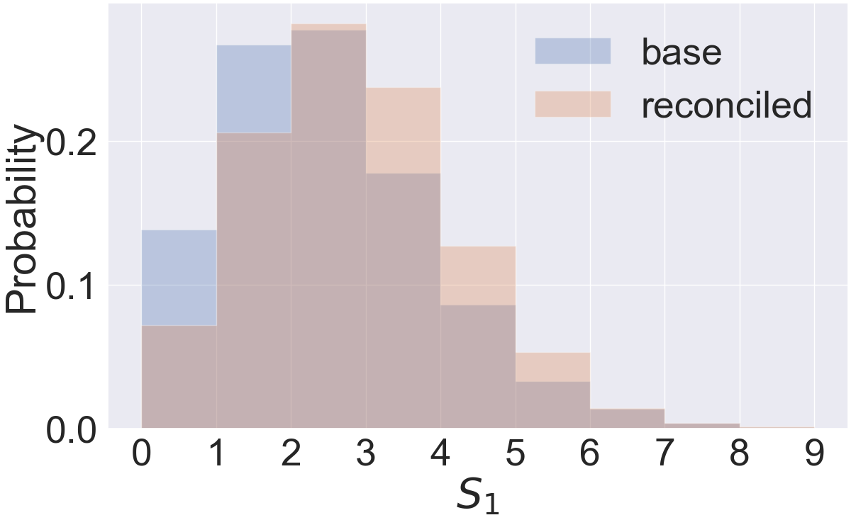
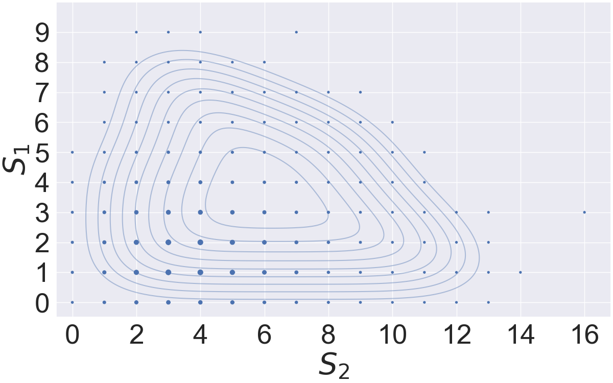
Figure 4: Left: The mean of $S_{1}$ increase after reconciliation. Right: $S_{1}$ and $S_{2}$ are negatively correlated after reconciliation.

The right plot of Figure 4 shows that $S_{1}$ and $S_{2}$ become negatively correlated after reconciliation. Indeed, $S_{1}$ and $S_{2}$ become dependent once $Y$ is observed, because $S_{1}+S_{2}=Y$. If for instance we observe $Y$=1, the only joint states compatible with the evidence are ($S_{1}=0,S_{2}=1$) and ($S_{1}=1,S_{2}=0$), whence the negative correlation. For the same reason, also virtual evidence induces negative correlation. Fig. 5 shows that the reconciled pmf of $Y$ is a compromise between its bottom-up pmf and its base forecast: this is an analogy with Bayesian inference, where the posterior distribution is a compromise between the prior and the likelihood of the observation.

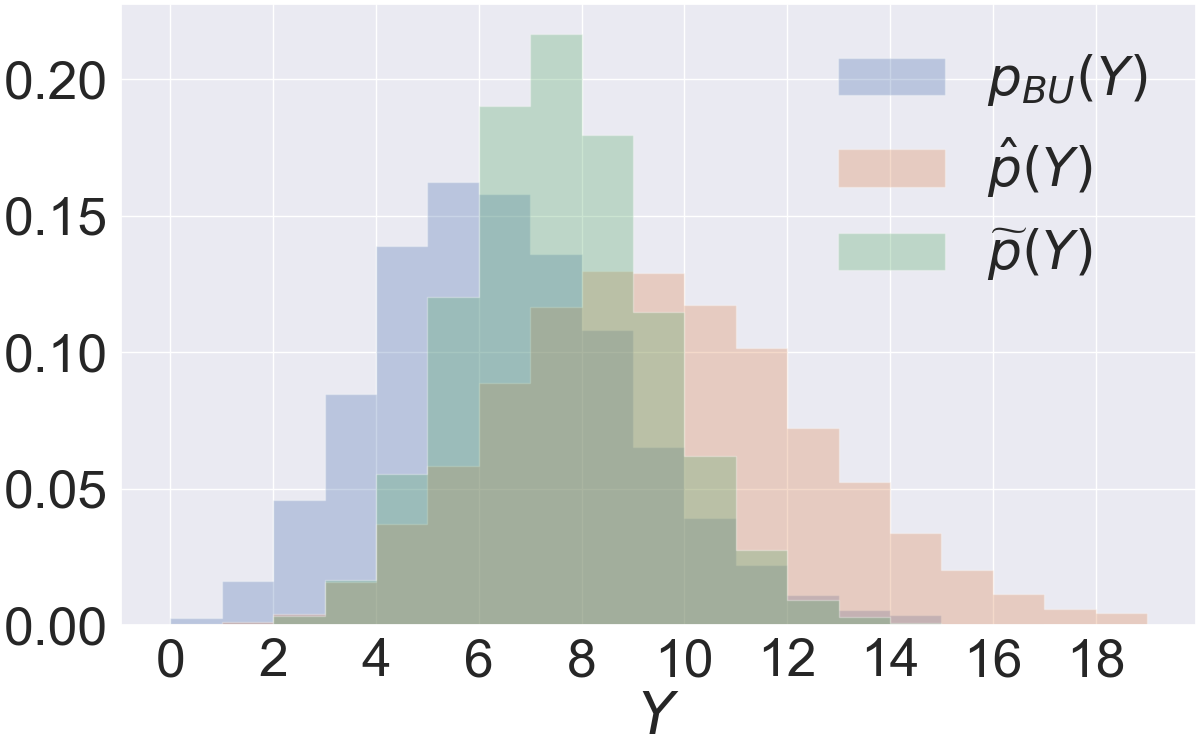
Figure 5: Bottom-up, base forecast and reconciled pmf of $Y$.

5 Experiments

We select time series with maximum value <30 and with average inter-demand interval (ADI) <2, which can be appropriately modelled by autoregressive models for counts. Following this criterion we select:

• 219 time series from carparts, available from the R package expsmooth [12] and regarding monthly sales of car parts;

• 53 time series from syph, available from the R package ZIM [33] and regarding the weekly number of syphilis cases in the United States, which we aggregate to the monthly scale (this step involve some approximation);

• 135 time series from hospital, available from the R package expsmooth [12] and regarding the monthly counts of patients.

In Table 4 we report the percentage of intermittent time series in each data set.

	selected	% intermittent	mean length
			(years)
carparts	219	94%	4
syph	53	47%	4
hospital	135	0%	7

Table 4: Main characteristics of the selected time series. We consider a time series as intermittent if its average inter-demand interval (ADI) is >1.32 [29].

Temporal hierarchy and base forecasts

In every experiment the bottom forecasts are at the monthly scale. As in [1], we compute the following temporal aggregates: 2-months, 3-months, 4-months, 6-months, 1 year.

At each level of the hierarchy we fit a GLM autoregressive model with negative binomial predictive distribution. We use the tscount package [20] and we select via BIC the order of the autoregression.

At every level of the hierarchy, the test set has length of one year. We thus compute forecasts up to $h$=12 steps ahead at the monthly level, up to $h$=6 steps ahead at the bi-monthly level, etc. The forecast of count time series models have closed form only one step ahead; after that, the predictive distribution is constituted by samples [20]. Depending on the reconciliation method being adopted, we fit a Gaussian or a negative binomial distribution on the samples.

Reconciliation

In the Gaussian case [4], the reconciled predictive distribution has the same mean and variance of minT (formulas (2) and (4) respectively) For Gaussian reconciliation, we fit a Gaussian distribution on the samples of the base forecast, for each level and for each forecasting horizon (e.g., we fit 12 different distributions at the monthly level). We then perform reconciliation using the covariance matrix of hierarchy variance and the structural scaling, discussed in Sec 2. These methods are referred to in the following as normal and structural scaling.

We moreover implemented a truncated approach. To this end we perform the normal reconciliation, truncating the distribution of the reconciled bottom forecast. We then sum them up via sampling in order to obtain the distribution of the upper variables. This a simple way to obtain positive reconciled forecasts.

We implement our approach by fitting a negative binomial distribution on the base forecasts on the samples of each level and each forecasting horizon and performing reconciliation via probabilistic programming. The probabilistic program contains 12 variables (the bottom variables) and 16 soft evidences, corresponding to the upper variables of the hierarchy. We refer to this methods as probCount. The reconciliation takes about 2-3 minutes on a standard laptop. This approach is therefore currently not suitable to hierarchies containing large number of variables. Alternative approaches based on importance sampling constitute a promising direction for efficient probabilistic reconciliation [34].

Indicators

We assess the methods according to their point forecasts, predictive distributions and prediction intervals. Let us denote by $y_{t+h}$ the actual value of the time series at time $t+h$ and by $\hat{y}_{t+h|t}$ the point forecast computed at time $t$ for time $t+h$. We further denote the predictive distribution by $\hat{f}_{t+h|t}$. Note that $\hat{f}_{t+h|t}(i)$ is a discrete probability mass for $i=1,\ldots,\infty$.

The mean scaled absolute error (MASE) [11] is defined as:

MAE $$=\frac{1}{h}\sum_{j=1}^{h}|y_{t+j}-\hat{y}_{t+j|t}|\,,$$

$$Q =\frac{1}{T-1}\sum_{t=2}^{T}|y_{t}-y_{t-1}|\,,$$

MASE $$=\frac{MAE}{Q}\,.$$

We use the median of the reconciled distribution as point forecast, since it is the optimal point forecasts for MAE and MASE [17]. However, the median point forecast is generally not coherent, even if the joint distribution is coherent [18].

Different scores for discrete predictive distributions are discussed in [17]. Here we use the ranked probability score (RPS). Given the predictive probability mass $\hat{f}_{t+h|t}(i)$, the cumulative predictive probability mass is $\hat{F}_{t+h|t}(k)=\sum_{i=0}^{k}\hat{f}_{t+h|t}(i)$. For a realization $y_{t+h}$, then we have:

$$\text{RPS}(\hat{f}_{t+h|t},y_{t+h})=\sum_{k=0}^{\infty}(\hat{F}_{t+h|t}(k)-\mathbb{1}_{y_{t+h}\leq k})^{2},$$ (13)

where $\mathbb{1}_{y\leq k}$ is the indicator function for $y\leq k$.

We compute the RPS of continuous distributions by applying the continuity correction, i.e. computing $p(X=x)$ as $\int_{x-0.5}^{x+0.5}g(t)dt$, where $g(t)$ denotes the continuous density.

We score the prediction intervals via the mean interval score (MIS) [8]. Let us denote by (1-$\alpha$) the desired coverage of the interval, by $l$ and $u$ the lower and upper bounds of the interval. We have:

$$\text{MIS}(l,u,y)=(u-l)+\frac{2}{\alpha}(l-y)\mathbb{1}(y<l)+\frac{2}{\alpha}(y-u)\mathbb{1}(y>u)\,.$$

We adopt a 90% coverage level ($\alpha$=0.1). The MIS rewards narrow prediction intervals; however, it also penalizes intervals which do not contain the actual value; the penalty depends on $\alpha$. In the definition of RPS and MIS, it is understood that $y_{t+j}$, $\hat{f}_{t+h|t}(i)$, $\hat{F}_{t+h|t}(k)$, $l$ and $u$ are specific for a certain level of the hierarchy and for a certain forecasting horizon $j$, $1\leq j\leq h$.

We also report the Energy score (ES), which is a proper scoring rule for distributions defined on the entire hierarchy [25]. Given a realization $\mathbf{y}$ and a joint probability $P$ on the entire hierarchy, the ES is:

$$ES(P,\mathbf{y})=E_{P}||\mathbf{y}-\mathbf{s}||^{\alpha}-\frac{1}{2}E_{P}||\mathbf{s}-\mathbf{s}^{*}||^{\alpha}\,,$$ (14)

where $\mathbf{s}$ and $\mathbf{s}^{*}$ are independent samples drawn from $P$. We compute the energy score using the scoringRules package [16] with $\alpha$=2.

Skill score

We compute the skill score on a certain indicator as the percentage improvement with respect to the normal method, taken as a baseline. Skill scores are scale-independent and can be thus averaged across multiple time series. For instance the skill score of probCount on MASE is:

$$\text{Skill (MASE, probCount)}=\frac{\text{MASE(normal) - MASE(probCount)}}{(\text{MASE(normal) + MASE(probCount)})/2}\,.$$

Thus a positive skill score implies an improvement compared to normal. The denominator makes the skill score symmetric and bounded between $-2$ and $2$, allowing a fair comparison between the competitors and the baseline.

For each level of the hierarchy, we compute the skill score for each forecasting horizon $j$ ($1\leq j\leq h$); then we average over the different $j$. Only for the probCount we compute also the skill score with respect to the base forecast, constituted by a negative binomial distribution fitted on the samples returned by the GLM models.

5.1 Experiments on carparts and syph

Skill score on carparts		vs normal			vs base
		struc scal	truncated	probCount	probCount
ENERGY SCORE		-0.06	-0.19	0.27	0.34
MASE	Monthly	-0.01	-0.02	0.18	0.00
	2-Monthly	-0.02	-0.08	0.21	0.00
	Quarterly	-0.03	-0.11	0.21	0.00
	4-Monthly	-0.03	-0.14	0.30	0.18
	Biannual	-0.04	-0.20	0.30	0.09
	Annual	-0.09	-0.30	0.89	0.80
	average	-0.04	-0.14	0.35	0.18
MIS	Monthly	0.00	0.27	0.36	0.38
	2-Monthly	0.00	-0.07	0.15	0.53
	Quarterly	-0.01	-0.21	0.15	0.58
	4-Monthly	-0.10	-0.29	0.17	0.67
	Biannual	-0.11	-0.27	0.20	0.85
	Annual	-0.24	-0.56	0.25	1.22
	average	-0.08	-0.19	0.22	0.71
RPS	Monthly	-0.02	-0.06	0.43	0.20
	2-Monthly	-0.03	-0.12	0.37	0.29
	Quarterly	-0.04	-0.15	0.40	0.25
	4-Monthly	-0.05	-0.20	0.42	0.33
	Biannual	-0.08	-0.27	0.32	0.43
	Annual	-0.12	-0.36	1.14	0.96
	average	-0.06	-0.19	0.51	0.41

(a) Results on time series extracted from carparts, detailed by each level of the hierarchy.

Skill score on syph		vs normal			vs base
		struc scal	truncated	probCount	probCount
ENERGY SCORE		-0.07	-0.21	0.27	0.28
MASE		-0.06	-0.17	0.35	0.06
MIS		-0.13	-0.16	0.20	0.23
RPS		-0.06	-0.18	0.42	0.41

(b) Results on time series extracted from syph, averaged over the entire hierarchy.

Table 5: Skill score on carparts and syph. The first columns report skill score with respect to normal. The last column reports the skill score of probCount with respect to the base forecasts.

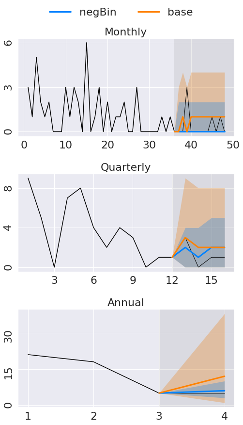
(a) Comparison of forecasts (base vs probCount) on a time series extracted from carparts.

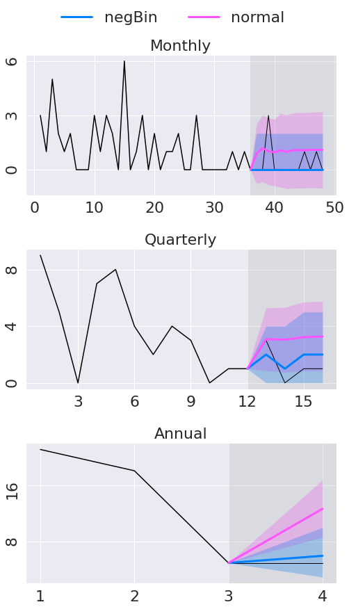
(b) Comparison of forecasts (normal vs probCount) on a time series extracted from carparts.

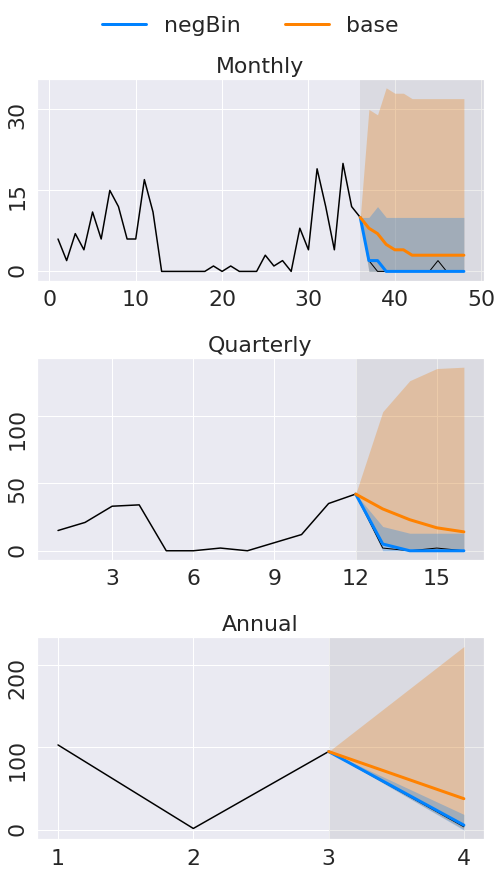
(c) Comparison of forecasts (base vs probCount) on a time series extracted from syph.

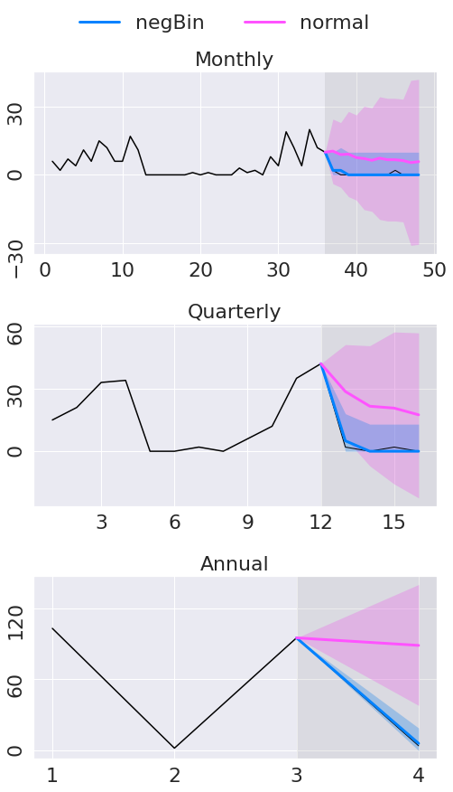
(d) Comparison of forecasts (normal vs probCount) on a time series extracted from syph.

Figure 6: Reconciliation of two time series from the carparts and the syph data set. For simplicity we only show three levels of the hierarchy. The black line shows the actual values.

The carparts data set has a high percentage of intermittent time series (94%) and the base forecasts are generally asymmetric. In these conditions probCount yields a large improvement over normal on every score (Table 5(a)). Averaging over the entire hierarchy, the improvement of probCount over normal ranges between 22% and 51% depending on the indicator; the energy score improves by about 27% The structural scaling and the truncated method perform worse than the normal method. Hence, the truncated method does not represent a satisfactory solution for modelling distributions over counts, even if it yields positive forecasts.

The forecast reconciled by probCount yield a large improvement also compared to the base forecast (last column of Table 5(a)). The largest improvements with respect to the base forecasts are in the highest level of the hierarchy, as already observed for temporal hierarchies [1].

Also in the syph data set, probCount largely outperforms normal on every indicator (Table 5(b)); the improvement varies between 27% and 42%. Large improvements are found also with respect to the base forecasts. The performance of both truncated and structural scaling is slightly worse than normal also in this case. The result for syph, detailed for each level of the hierarchy, are given in the appendix.

In Figure 6 we provide two examples of reconciliation, taken from carparts and syph respectively. In both examples, the distribution of the base forecasts is asymmetric at every level (Figures 6(a), 6(b)), with the median much lower than the mid-point of the prediction interval. Based on this information, probCount revises downwards the point forecasts compare to the base forecasts. At the monthly level its point forecasts (i.e., the medians) are 0. This is both the lower bound of the prediction interval and the median: the reconciled distribution is strongly asymmetric as it can happen when the counts are low. The adjustment applied by probCount is effective, and its point forecasts are more accurate than the base forecasts at every level of the hierarchy.

The normal method does not capture the asymmetry of the base forecasts. Its reconciled point forecasts are less accurate than those of probCount, and its prediction intervals often include negative values (Figures 6(b), 6(d)).

Both probCount and normal have shorter prediction intervals compared to the base forecast. This makes the predictive distribution and the prediction interval more informative, increasing the MIS and the RPS score. Yet, the prediction intervals of both probCount and normal are sometimes too short. In future, this could be addressed by modelling the correlation between the base forecasts using more sophisticated multivariate distributions over counts [24, 14].

5.2 Experiments on hospital

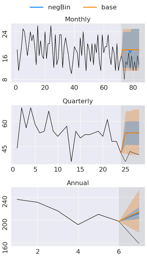
(a) Comparison of forecasts (base vs probCount) on a time series from hospital.

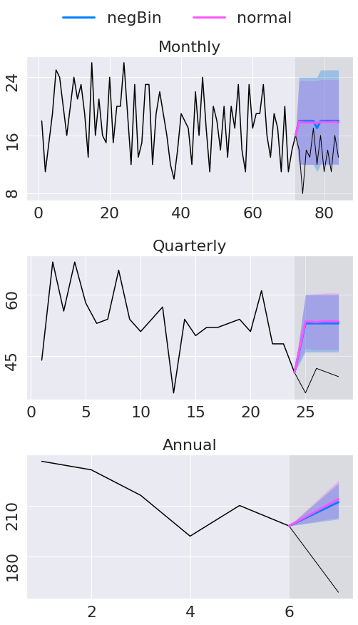
(b) Comparison of forecasts (normal vs probCount) on a time series from hospital.

Figure 7: Examples of reconciliation on a time series from the hospital data set.

Skill score on hospital		Skill score vs normal			vs base
		struc scal	truncated	probCount	probCount
ENERGY SCORE		-0.02	0.00	0.00	0.03
MASE		0.00	0.00	-0.02	0.01
MIS		-0.02	0.00	0.00	0.03
RPS		-0.01	0.00	0.00	0.04

Table 6: Skill score on time series from hospital, averaged over the entire hierarchy.

All the time series extracted from the hospital data set are smooth; the values are high enough to yield symmetric prediction intervals. The samples of the base forecast are well fit both by the negative binomial and by the Gaussian distribution, among which there are little differences. Thus the reconciliation methods become practically equivalent (Figure 7(b)), yielding an almost identical performance (Table 6). The utility of temporal reconciliation is confirmed by the positive skill scores compared to the base forecasts.

6 Conclusions

We have shown that virtual evidence, a method originally developed for conditioning probabilistic graphical models on uncertain evidence, can be used to perform probabilistic reconciliation in a principled fashion. Our method can reconcile real-valued and count time series; we focus however on the latter case, which is especially important since there are currently no methods for reconciling count time series.

The most important result of this paper is that our approach consistently provides a major improvement, compared to Gaussian probabilistic reconciliation, in the reconciliation of intermittent time series, which are notoriously hard to forecast. Future research directions include modelling the correlation between the base forecasts and developing a faster sampling approach in order to reconcile large hierarchies.

Appendix A Reconciliation of a 4-2-1 hierarchy

The 4-2-1 hierarchy of Fig.1 is reconciled by the code below:

⬇

1 def reconcile (lambda1, lambda2, lambdaY):

2 import pymc3 as pm

3 basic_model = pm.Model()

4 with basic_model:

5 #base forecast of the bottom variables

6 Q1 = pm.Poisson (’Q1’, mu = lambda1)

7 Q2 = pm.Poisson (’Q2’, mu = lambda2)

8 Q3 = pm.Poisson (’Q3’, mu = lambda3)

9 Q4 = pm.Poisson (’Q4’, mu = lambda4)

10

11 #Virtual evidence of the upper variables

12 S1 = pm.Poisson (’S1’, mu = lambda_S1, observed = S1 + S2)

13 S2 = pm.Poisson (’S2’, mu = lambda_S2, observed = S3 + S4)

14 Y = pm.Poisson (’Y’, mu = lambda_Y, observed = S1+S2+S3+S4)

15

16 #sampling the posterior, i.e., the reconciled distribution

17 #for each (s1, s2) computes p(s1) p(s2) p(Y=s1+s2)

18 #and eventually normalizes

19 trace = pm.sample()

20 return trace

Appendix B Equivalence of definitions 5 and 2 in the continuous case

Proposition 2.

Definitions 5 and 2 are equivalent in the continuous case.

Proof.

In the continuous case $\mathcal{X}=\mathbb{R}$, thus for any $\mathcal{B}\in\mathcal{F}_{\mathcal{X}^{m}}$, $s(\mathcal{B})=\{s(\mathbf{b}):\mathbf{b}\in\mathcal{B}\}$. We have that $s(\mathcal{B})\in\mathcal{F}_{\mathfrak{s}}$ because $\forall\mathbf{b}\in\mathcal{B}$, $s(\mathbf{b})\in\mathfrak{s}$, by definition, and $\mathcal{F}_{\mathfrak{s}}\subseteq\mathcal{F}_{s(\mathcal{X}^{m})}$.

On the other hand, given a element $\mathcal{A}\in\mathcal{F}_{\mathfrak{s}}$, we can always find a set $\tilde{\mathcal{B}}\in\mathcal{F}_{\mathcal{X}^{m}}$ such that $s(\tilde{\mathcal{B}})=\mathcal{A}$. In fact, for any $\mathbf{a}\in\mathcal{A}$ we can write $\mathbf{a}=[\mathbf{a}_{upp},\mathbf{a}_{bot}]$ and $\mathbf{a}_{upp}=S\mathbf{a}_{bot}$ by definition. Thus if we take $\tilde{\mathbf{b}}=\mathbf{a}_{bot}$ we have $s(\tilde{\mathbf{b}})=\mathbf{a}$. So we have that $\mathcal{A}\in\mathcal{F}_{s(\mathcal{X}^{m})}$.

Since we have showed that the two $\sigma$-algebras $\mathcal{F}_{\mathfrak{s}}$ and $\mathcal{F}_{s(\mathcal{X}^{m})}$ are equivalent and the measures $\check{\nu}_{\mathfrak{s}}$ and $\check{\nu}$ take the same values on all sets of $\mathcal{F}_{\mathcal{X}^{m}}$ we have that def. 5 and def. 2 are equivalent in the continuous case. ∎

Appendix C Additional fine-grained results on syph and hospital

Skill score on syph		vs normal			vs base
		struc scal	truncated	probCount	probCount
MASE	Monthly	-0.07	-0.13	0.43	0.03
	2-Monthly	-0.08	-0.16	0.40	0.09
	Quarterly	-0.08	-0.17	0.37	0.07
	4-Monthly	-0.07	-0.18	0.35	0.07
	Biannual	-0.07	-0.17	0.36	0.10
	Annual	-0.02	-0.19	0.20	0.01
	average	-0.06	-0.17	0.35	0.06
MIS	Monthly	-0.07	0.21	0.38	0.41
	2-Monthly	-0.16	-0.09	0.19	0.33
	Quarterly	-0.16	-0.18	0.13	0.29
	4-Monthly	-0.17	-0.27	0.17	0.25
	Biannual	-0.11	-0.25	0.21	0.14
	Annual	-0.10	-0.38	0.14	-0.03
	average	-0.13	-0.16	0.20	0.23
RPS	Monthly	-0.05	-0.20	0.62	0.55
	2-Monthly	-0.07	-0.18	0.49	0.49
	Quarterly	-0.05	-0.15	0.41	0.44
	4-Monthly	-0.05	-0.16	0.40	0.42
	Biannual	-0.08	-0.20	0.39	0.37
	Annual	-0.04	-0.17	0.21	0.22
	average	-0.06	-0.18	0.42	0.41

Skill score on hospital		normal			vs base
		struc scal	truncated	probCount	probCount
MASE	Monthly	0.00	0.00	0.00	0.00
	2-Monthly	0.00	0.00	0.00	0.00
	Quarterly	0.00	0.00	-0.02	0.00
	4-Monthly	0.00	0.00	-0.01	0.00
	Biannual	0.00	0.00	0.00	0.00
	Annual	0.00	0.00	-0.07	0.04
	average	0.00	0.00	-0.02	0.01
MIS	Monthly	0.01	0.00	0.01	0.12
	2-Monthly	0.00	0.00	0.00	0.15
	Quarterly	0.00	0.00	0.00	0.17
	4-Monthly	-0.02	0.00	0.01	0.16
	Biannual	-0.04	0.00	0.00	-0.05
	Annual	-0.07	0.00	0.00	-0.38
	average	-0.02	0.00	0.00	0.03
RPS	Monthly	0.00	0.00	0.02	0.05
	2-Monthly	0.00	0.00	0.00	0.09
	Quarterly	0.00	0.00	-0.01	0.09
	4-Monthly	-0.01	0.00	0.00	0.05
	Biannual	-0.02	0.00	0.05	0.01
	Annual	-0.03	0.00	-0.08	-0.08
	average	-0.01	0.00	0.00	0.04

Proof of Proposition 1

Proof.

We prove this by induction over the number of upper time series $n-m$.

Note that if we have one upper time series the two procedures are the same.

Assume that the two procedures are the same for $n-m-1$ upper time series, i.e. the sequential update after $n-m-1$ upper time series forecasts reconciliations is $\tilde{p}_{n-m-1}(\mathbf{y})=\mathds{1}_{\mathbf{A}\mathbf{b}}(\mathbf{u})\dfrac{\sum_{\mathbf{u}^{*}_{-1}}p_{BU}(\mathbf{u}^{*}_{-1},\mathbf{b})\hat{p}(\mathbf{u}^{*}_{-1})}{\sum_{\mathbf{u}^{*}_{-1}}\sum_{\mathbf{b}^{*}}p_{BU}(\mathbf{u}^{*}_{-1},\mathbf{b})\hat{p}(\mathbf{u}^{*}_{-1})}$, where we denote by $\mathbf{u}^{*}_{-1}$ a generic value for the pmf of the first $n-m-1$ upper forecasts.

The next sequential update is

$$\tilde{p}_{n-m}(\mathbf{b})=\dfrac{\sum_{{u}^{*}_{n-m}}\tilde{p}_{n-m-1}({u}^{*}_{n-m},\mathbf{b})\hat{p}({u}^{*}_{n-m})}{\sum_{{u}^{*}_{n-m}}\sum_{\mathbf{b}^{*}}\mathds{1}_{\mathbf{A}[n-m,]\mathbf{b}}({u}^{*}_{n-m})\tilde{p}_{n-m-1}(\mathbf{b})\hat{p}({u}^{*}_{n-m})}.$$

We denote the denominator as $Z_{n-m}$, a normalizing constant, and we study just the numerator $\tilde{p}_{n-m}(\mathbf{b})Z_{n-m}$.

$$\tilde{p}_{n-m}(\mathbf{b})Z_{n-m} =\sum_{{u}^{*}_{n-m}}\tilde{p}_{n-m-1}({u}^{*}_{n-m},\mathbf{b})\hat{p}({u}^{*}_{n-m})$$

$$=\sum_{{u}^{*}_{n-m}}\mathds{1}_{\mathbf{A}[n-m,]\mathbf{b}}({u}^{*}_{n-m})\tilde{p}_{n-m-1}(\mathbf{b})\hat{p}({u}^{*}_{n-m})$$

$$=\sum_{{u}^{*}_{n-m}}\mathds{1}_{\mathbf{A}[n-m,]\mathbf{b}}({u}^{*}_{n-m})\dfrac{\sum_{\mathbf{u}^{*}_{-1}}p_{BU}(\mathbf{u}^{*}_{-1},\mathbf{b})\hat{p}(\mathbf{u}^{*}_{-1})}{Z_{n-m-1}}\hat{p}({u}^{*}_{n-m}),$$ (15)

where we denote by $Z_{n-m-1}$ the normalizing constant for the reconciled distribution after $n-m-1$ updates. Note that $p_{BU}(\mathbf{u}^{*}_{-1},\mathbf{b})=\mathds{1}_{\mathbf{A}[-1,]\mathbf{b}}(\mathbf{u}^{*}_{-1})\hat{p}(\mathbf{b})$, where $\mathbf{A}[-1,]$ indicates all but the last row of the matrix $\mathbf{A}$. Moreover

$$\mathds{1}_{\mathbf{A}[-1,]\mathbf{b}}(\mathbf{u}^{*}_{-1})\mathds{1}_{\mathbf{A}[n-m,]\mathbf{b}}({u}^{*}_{n-m})=\mathds{1}_{\mathbf{A}\mathbf{b}}({u}^{*}),$$

if $\mathbf{u}^{*}=[\mathbf{u}^{*}_{-1}\ u^{*}_{n-m}]$. Therefore the double sum in equation (15) can be simplified as

$$\tilde{p}_{n-m}(\mathbf{b})Z_{n-m} =\dfrac{\sum_{\mathbf{u}^{*}=[\mathbf{u}^{*}_{-1}\ {u}^{*}_{n-m}]}\mathds{1}_{\mathbf{A}\mathbf{b}}(\mathbf{u}^{*})\hat{p}(\mathbf{b})\hat{p}(\mathbf{u}^{*}_{-1})\hat{p}({u}^{*}_{n-m})}{Z_{n-m-1}}$$

$$=\dfrac{\sum_{\mathbf{u}^{*}=[\mathbf{u}^{*}_{-1}\ {u}^{*}_{n-m}]}p_{BU}(\mathbf{u}^{*},\mathbf{b})\hat{p}(\mathbf{u}^{*}_{-1})\hat{p}({u}^{*}_{n-m})}{Z_{n-m-1}}$$

Since the upper time series forecast is conditionally independent we have $\hat{p}(\mathbf{u}^{*})=\hat{p}(\mathbf{u}^{*}_{-1})\hat{p}({u}^{*}_{n-m})$ and thus we obtain the result.

∎

References

- Athanasopoulos et al. [2017] Athanasopoulos, G., Hyndman, R.J., Kourentzes, N., Petropoulos, F.. Forecasting with temporal hierarchies. European Journal of Operational Research 2017;262(1):60–74.
- Carpenter et al. [2017] Carpenter, B., Gelman, A., Hoffman, M.D., Lee, D., Goodrich, B., Betancourt, M., Brubaker, M., Guo, J., Li, P., Riddell, A.. Stan: A probabilistic programming language. Journal of Statistical Software, Articles 2017;76(1):1–32. URL: https://www.jstatsoft.org/v076/i01.
- Chan and Darwiche [2005] Chan, H., Darwiche, A.. On the revision of probabilistic beliefs using uncertain evidence. Artificial Intelligence 2005;163(1):67–90.
- Corani et al. [2020] Corani, G., Azzimonti, D., Augusto, J.P., Zaffalon, M.. Probabilistic reconciliation of hierarchical forecast via Bayes’ rule. In: Proc. European Conf. On Machine Learning and Knowledge Discovery in Database ECML/PKDD. volume 3; 2020. p. 211–226.
- Darwiche [2009] Darwiche, A.. Modeling and reasoning with Bayesian networks. Cambridge university press, 2009.
- Di Fonzo and Girolimetto [2022] Di Fonzo, T., Girolimetto, D.. Forecast combination-based forecast reconciliation: Insights and extensions. International Journal of Forecasting 2022;doi:https://doi.org/10.1016/j.ijforecast.2022.07.001.
- Durrant-Whyte and Henderson [2016] Durrant-Whyte, H., Henderson, T.C.. Multisensor data fusion. Springer handbook of robotics 2016;:867–896.
- Gneiting [2011] Gneiting, T.. Quantiles as optimal point forecasts. International Journal of forecasting 2011;27(2):197–207.
- Hollyman et al. [2021] Hollyman, R., Petropoulos, F., Tipping, M.E.. Understanding forecast reconciliation. European Journal of Operational Research 2021;294(1):149–160.
- Hollyman et al. [2022] Hollyman, R., Petropoulos, F., Tipping, M.E.. Hierarchies everywhere–managing & measuring uncertainty in hierarchical time series. arXiv preprint arXiv:220915583 2022;.
- Hyndman [2006] Hyndman, R.. Another look at forecast-accuracy metrics for intermittent demand. Foresight: The International Journal of Applied Forecasting 2006;4(4):43–46.
- Hyndman [2015] Hyndman, R.J.. expsmooth: Data Sets from ”Forecasting with Exponential Smoothing”, 2015. URL: https://CRAN.R-project.org/package=expsmooth; r package version 2.3.
- Hyndman et al. [2011] Hyndman, R.J., Ahmed, R.A., Athanasopoulos, G., Shang, H.L.. Optimal combination forecasts for hierarchical time series. Computational Statistics & Data Analysis 2011;55(9):2579 – 2589.
- Inouye et al. [2017] Inouye, D.I., Yang, E., Allen, G.I., Ravikumar, P.. A review of multivariate distributions for count data derived from the Poisson distribution. Wiley Interdisciplinary Reviews: Computational Statistics 2017;9(3).
- Jeon et al. [2019] Jeon, J., Panagiotelis, A., Petropoulos, F.. Probabilistic forecast reconciliation with applications to wind power and electric load. European Journal of Operational Research 2019;279(2):364–379.
- Jordan et al. [2019] Jordan, A., Krüger, F., Lerch, S.. Evaluating probabilistic forecasts with scoringRules. Journal of Statistical Software 2019;90(12):1–37.
- Kolassa [2016] Kolassa, S.. Evaluating predictive count data distributions in retail sales forecasting. International Journal of Forecasting 2016;32(3):788–803.
- Kolassa [2022] Kolassa, S.. Do we want coherent hierarchical forecasts, or minimal mapes or maes?(we won’t get both!). International Journal of Forecasting 2022;doi:https://doi.org/10.1016/j.ijforecast.2022.11.006.
- Kourentzes and Athanasopoulos [2021] Kourentzes, N., Athanasopoulos, G.. Elucidate structure in intermittent demand series. European Journal of Operational Research 2021;288(1):141–152.
- Liboschik et al. [2017] Liboschik, T., Fokianos, K., Fried, R.. tscount: An R package for analysis of count time series following generalized linear models. Journal of Statistical Software 2017;82(5):1–51.
- Martin [2018] Martin, O.. Bayesian analysis with Python: introduction to statistical modeling and probabilistic programming using PyMC3 and ArviZ. Packt Publishing Ltd, 2018.
- Munk et al. [2022] Munk, A., Mead, A., Wood, F.. Uncertain evidence in probabilistic models and stochastic simulators. arXiv preprint arXiv:221012236 2022;.
- Nystrup et al. [2020] Nystrup, P., Lindström, E., Pinson, P., Madsen, H.. Temporal hierarchies with autocorrelation for load forecasting. European Journal of Operational Research 2020;280(3):876–888.
- Panagiotelis et al. [2012] Panagiotelis, A., Czado, C., Joe, H.. Pair copula constructions for multivariate Discrete Data. Journal of the American Statistical Association 2012;107(499):1063–1072.
- Panagiotelis et al. [2023] Panagiotelis, A., Gamakumara, P., Athanasopoulos, G., Hyndman, R.J.. Probabilistic forecast reconciliation: Properties, evaluation and score optimisation. European Journal of Operational Research 2023;306(2):693–706.
- Pearl [1988] Pearl, J.. Probabilistic reasoning in intelligent systems: networks of plausible inference. Morgan kaufmann, 1988.
- Rangapuram et al. [2021] Rangapuram, S.S., Werner, L.D., Benidis, K., Mercado, P., Gasthaus, J., Januschowski, T.. End-to-end learning of coherent probabilistic forecasts for hierarchical time series. In: Proc. 38th Int. Conference on Machine Learning (ICML). 2021. p. 8832–8843.
- Salvatier et al. [2016] Salvatier, J., Wiecki, T.V., Fonnesbeck, C.. Probabilistic programming in Python using PyMC3. PeerJ Computer Science 2016;2:e55.
- Syntetos and Boylan [2005] Syntetos, A.A., Boylan, J.E.. The accuracy of intermittent demand estimates. International Journal of Forecasting 2005;21(2):303–314.
- Taieb et al. [2021] Taieb, S.B., Taylor, J.W., Hyndman, R.J.. Hierarchical probabilistic forecasting of electricity demand with smart meter data. Journal of the American Statistical Association 2021;116(533):27–43.
- Wickramasuriya et al. [2019] Wickramasuriya, S.L., Athanasopoulos, G., Hyndman, R.J.. Optimal forecast reconciliation for hierarchical and grouped time series through trace minimization. Journal of the American Statistical Association 2019;114(526):804–819.
- Wickramasuriya et al. [2020] Wickramasuriya, S.L., Turlach, B.A., Hyndman, R.J.. Optimal non-negative forecast reconciliation. Statistics and Computing 2020;30(5):1167–1182.
- Yang et al. [2018] Yang, M., Zamba, G., Cavanaugh, J.. ZIM: Zero-Inflated Models (ZIM) for Count Time Series with Excess Zeros, 2018. URL: https://CRAN.R-project.org/package=ZIM; r package version 1.1.0.
- Zambon et al. [2022] Zambon, L., Azzimonti, D., Corani, G.. Efficient probabilistic reconciliation of forecasts for real-valued and count time series. arXiv 2022;doi:10.48550/ARXIV.2210.02286.