funcharts: Control charts for multivariate functional data in R

Christian Capezza, Fabio Centofanti, Antonio Lepore, Biagio Palumbo, Alessandra Menafoglio, Simone Vantini funcharts: Control charts for multivariate functional data in R funcharts: Control charts for multivariate functional data in R Modern statistical process monitoring (SPM) applications focus on profile monitoring, i.e., the monitoring of process quality characteristics that can be modeled as profiles, also known as functional data. Despite the large interest in the profile monitoring literature, there is still a lack of software to facilitate its practical application. This article introduces the funcharts R package that implements recent developments on the SPM of multivariate functional quality characteristics, possibly adjusted by the influence of additional variables, referred to as covariates. The package also implements the real-time version of all control charting procedures to monitor profiles partially observed up to an intermediate domain point. The package is illustrated both through its built-in data generator and a real-case study on the SPM of Ro-Pax ship CO₂ emissions during navigation, which is based on the ShipNavigation data provided in the Supplementary Material. functional data analysis, statistical process control, profile monitoring, multivariate functional linear regression, R functional data analysis, statistical process control, profile monitoring, multivariate functional linear regression, R

1 Introduction

Recent acquisition technologies are based on multiple and high-frequency sensors installed on board of devices or machines and allow the acquisition of a large amount of data about many process variables and quality characteristics. In this context, statistical process monitoring (SPM) calls for methods able to model and analyze quality characteristics in the form of multiple curves, i.e., continuous functions defined on compact sets often referred to as functional data or profiles. For details on functional data analysis (FDA), the reader is referred to ramsay2005functional; horvath2012inference; ferraty2006nonparametric; kokoszka2017introduction. The large availability of functional data is leading to a growing interest in profile monitoring (noorossana2011statistical), which aims to check the stability over time of the process based on observations of one or more functional quality characteristics of interest, that is, as in the traditional SPM, to test whether or not the process is affected also by special and not only by common causes of variations. In the former case, the process is said to be out of control (OC), while in the latter case, it is said to be in control (IC). One of the first reviews on this topic is the paper of woodall2004using. For other relevant contributions, see jin1999feature, colosimo2010comparison, grasso2016using, grasso2017phase, menafoglio2018profile, maleki2018overview, and jones2021practitioners.

The available approaches to profile monitoring are generally based on building control charts capable of detecting OC conditions, without necessarily considering the relationship between the quality characteristic and variables that may have an influence on it, referred to as covariates. A few exceptions are the recent works of capezza2020control and centofanti2020functional, who propose methods to extend the regression control chart (mandel1969regression) to functional data settings, where the quality characteristic is influenced by scalar or functional covariates, with the aim to improve the effectiveness of the monitoring strategy. In particular, they propose a control charting scheme based on the residuals of a linear regression with multivariate functional covariates used as regressors and the scalar (capezza2020control) or functional quality characteristics used as the response (centofanti2020functional).

Surprisingly, despite the large interest in the profile monitoring literature, there is a lack of software specifically designed for this type of application in modern data-rich scenarios. The qcc R package (scrucca2017qcc), which is one of the most popular for the SPM, focuses indeed on control charts for univariate and multivariate data, only. Also in the context of batch process monitoring, the dvqcc (valk2020dvqcc) R package provides a nice set of control charts based on the vector autoregressive model (marcondes2020dynamic) related to monitoring multiple variables observed over time but requires aligned data, while often profiles are observed over irregular grids with a different number of discrete points for each curve. Moreover, none of the aforementioned packages implement SPM methods able to account for one or more covariates, possibly functional, which may influence the quality characteristic of interest.

The funcharts R package introduced in this work and available on CRAN (capezza2021funcharts) is instead the first off-the-shelf toolkit able to perform SPM of functional quality characteristics alone or adjusted by the influence of covariates. In particular, in the former case, we provide the implementation of the methodology proposed in colosimo2010comparison for profile monitoring of univariate functional data based on functional principal component analysis and its extension to the case of multivariate functional data. Whereas, in the latter case, we implement the aforementioned methods proposed by capezza2020control and centofanti2020functional. The funcharts package focuses on the prospective monitoring of the process, referred to as Phase II. That is, given a clean data set with $n$ observations assumed to be representative of IC process performance, referred to as reference data set, the objective is to build appropriate control charts able to issue an alarm when the process is OC based on future individual observations drawn from it, hereinafter referred to as OC observations. Accordingly, we will refer to any future individual observations drawn from the IC process as IC observations.

In all the considered settings, the funcharts package implements also a real-time version of the functional control charts by accepting as input also profiles that are partially observed up to an intermediate domain point and adapting the real-time monitoring originally proposed by capezza2020control in the case of scalar response to the case of functional response.

The remainder of this article is organized as follows. Section 2 briefly overviews the methods that are implemented in the funcharts package. Comprehensive usage of the funcharts package is covered with a built-in simulation example in Section 3 and a real-case study in the monitoring of CO₂ emissions of a Ro-Pax ship during navigation in Section LABEL:sec_realcasestudy. Section LABEL:sec_conclusions concludes this article.

2 Overview of the methods implemented in funcharts

This section provides details of the methods implemented in funcharts. Section 2.1 describes how multivariate functional principal component analysis (MFPCA) is performed to represent functional data. Section 2.2 reviews the methodologies for SPM of multivariate functional data without covariates and extends the method proposed by colosimo2010comparison for univariate profiles to the multivariate setting. The control charts proposed by capezza2020control and centofanti2020functional are introduced in Section 2.3.1 and 2.3.2, respectively. Finally, in Section 2.4, the real-time implementation of these methods is illustrated.

2.1 Multivariate functional principal component analysis

Let $\bm{X}_{i}=\{(X_{i1},\dots,X_{iP})^{\top}\}_{i=1,\dots,n}$ denote $n$ observations of a vector of $P$ functional variables, in the Hilbert space $L^{2}(\mathcal{T})^{P}$, whose components $X_{i1},\dots X_{iP}$ belong to $L^{2}(\mathcal{T})$, the space of square integrable functions defined on the compact interval $\mathcal{T}$. More specifically, the funcharts package assumes that these functional data are densely observed on a set of discrete grid points (usually in time or space) and can be represented through cubic B-spline basis expansion with order four and equally spaced knots. The B-spline basis system has shown to enjoy remarkable theoretical as well as computational properties in the problem of recovering a smooth signal from noisy measurements (de1978practical; wahba1990spline; green1994nonparametric). To get a functional observation from the discrete grid points, a large number of basis functions is chosen and basis coefficients are estimated using penalized least squares. The penalty term is the integrated squared second derivative with smoothing parameter selected through generalized cross-validation (GCV) (ramsay2005functional).

MFPCA (ramsay2005functional; jacques2014model; happ2018multivariate) is then used to get a finite representation of functional data. Moreover, to take into account the possible different ranges of variation of the $P$ functional variables, these are empirically standardized, as in chiou2014multivariate, i.e., by firstly subtracting pointwise from each original variable the corresponding sample mean function and then dividing the result pointwise by the relative sample standard deviation function. Then, MFPCA consists in finding the eigenvalues $\lambda_{m}$ and the corresponding eigenfunctions $\bm{\psi}_{m}=(\psi_{m1},\dots,\psi_{mP})^{\top}\in L^{2}(\mathcal{T})^{P}$, with $1\leq m\leq n-1$, as the solutions of the eigenvalue equation

$$\int_{\mathcal{T}}\bm{V}(s,t)\bm{\psi}_{m}(s)ds=\lambda_{m}\bm{\psi}_{m}(t),\quad\forall t\in\mathcal{T},$$ (1)

where $\bm{V}(s,t)=\frac{1}{n-1}\sum_{i=1}^{n}\bm{X}_{i}(s)\bm{X}_{i}(t)^{\top}$ is the empirical covariance function of the multivariate functional data. Eigenvalues are arranged in a non-increasing order, i.e. $\lambda_{1}\geq\lambda_{2}\geq\dots\geq 0$. Eigenfunctions are orthogonal to each other, i.e., $\sum_{p=1}^{P}\int_{\mathcal{T}}\psi_{m_{1}p}(t)\psi_{m_{2}p}(t)dt=\mathbbm{1}(m_{1}=m_{2})$, where $\mathbbm{1}(\cdot)$ is the indicator function, and are also known as multivariate functional principal components, or principal components (PCs). For computational details, the reader is referred to Section 8.4.2 of ramsay2005functional. By projecting each observation onto the the PCs, we get the multivariate functional PC scores, or simply scores $\xi_{im}=\sum_{p=1}^{P}\int_{\mathcal{T}}X_{ip}(t)\psi_{mp}(t)dt$, which accordingly satisfy $\sum_{i=1}^{n}\xi_{im}=0$ and $\sum_{i=1}^{n}\xi_{im_{1}}\xi_{im_{2}}/(n-1)=\lambda_{m_{1}}\mathbbm{1}(m_{1}=m_{2})$.

A finite representation of the original data is obtained by retaining a finite subset of the PCs. In the following, we consider the most popular choice to retain the first $M$ PCs, i.e., the ones associated with the largest $M$ eigenvalues. Alternative choices are discussed in capezza2020control. Thus, $\bm{X}_{i}$ is approximated with $\hat{\bm{X}_{i}}=(\hat{X}_{i1},\dots,\hat{X}_{iP})^{\top}$, defined as

$$\hat{X}_{ip}\left(t\right)=\sum_{m=1}^{M}\xi_{im}\psi_{mp}\left(t\right),\quad t\in\mathcal{T},p=1,\dots,P.$$ (2)

2.2 Functional control charts for multivariate quality characteristics

Let us consider a vector of $P$ functional variables as a functional quality characteristics of interest to be monitored. To this aim, for each observation $\{\bm{X}_{i}\in L^{2}(\mathcal{T})^{P}\}_{i=1,\dots,n}$, two control charts are respectively built on the Hotelling’s $T^{2}$ and squared prediction error ($SPE$) statistics, defined as

$$T_{i}^{2}=\sum_{m=1}^{M}\xi_{im}^{2}/\lambda_{m},\quad SPE_{i}=\sum_{p=1}^{P}\int_{\mathcal{T}}(X_{ip}(t)-\hat{X}_{ip}(t))^{2}dt.$$ (3)

where the $SPE$ statistic can be also calculated as $SPE_{i}=\sum_{M+1}^{n-1}\xi_{m}^{2}$. The Hotelling’s $T^{2}$ statistic monitors $\hat{\bm{X}_{i}}$ defined in Equation (2) through the retained PCs, while the $SPE$ statistic monitors the approximation error due to the dimension reduction. While in colosimo2010comparison control chart limits $T^{2}_{lim}$ and $SPE_{lim}$ are calculated based on the assumption that scores are normally distributed, in the funcharts package they are calculated non-parametrically by means of empirical quantiles of the reference data set distribution of the Hotelling’s $T^{2}$ and $SPE$ statistics. The funcharts package uses the Bonferroni correction (hsu1996multiple) to constrain the family-wise error rate to be smaller than a desired value $\alpha\in(0,1)$ by setting the Type I error rate in each of the two control charts equal to $\alpha/2$, that for each control chart is the nominal probability that an in-control point falls outside of the control limits. Moreover, as shown in capezza2020control, the Hotelling’s $T^{2}$ and $SPE$ statistics can be decomposed as sums over the $P$ functional variables. In this way, the contributions of the $p$-th variable, $p=1,\dots,P$, of the $i$-th observation, $i=1,\dots,n$, to each monitoring statistic can be, respectively, measured by $CONT_{T^{2}_{i},p}$ and $CONT_{SPE_{i},p}$ as follows

$$CONT_{T^{2}_{i},p}=\sum_{m=1}^{M}\frac{\xi_{im}}{\lambda_{m}}\int_{\mathcal{T}}X_{ip}(t)\psi_{mp}(t)dt,\quad CONT_{SPE_{i},p}=\int_{\mathcal{T}}(X_{ip}(t)-\hat{X}_{ip}(t))^{2}dt.$$ (4)

These quantities allow to identify which functional variables have been responsible of especially large values of a monitoring statistic and are then an important tool for fault detection. capezza2020control noted that these contribution terms may have very different variability, for each $p=1,\dots,P$. Therefore, large variable contributions are identified as those that exceed the relative empirical upper limits.

Let us denote by $\bm{X}^{*}=(X^{*}_{1},\dots,X^{*}_{P})^{\top}$ a future observation to be monitored in Phase II. After standardization with respect to the sample mean and standard deviation functions calculated on the reference data set, scores are calculated by projecting $\bm{X}^{*}$ onto the the PCs. This allows one to calculate the approximation $\hat{\bm{X}}^{*}$ using Equation (2) and the two monitoring statistics, which we denote as $T^{2*}$ and $SPE^{*}$, using Equation (3). If either the $T^{2*}$ or $SPE^{*}$ monitoring statistic observation is larger than the corresponding control limit, an alarm is issued. Then, contributions to the OC monitoring statistic are calculated through Equation (4) and variables with a contribution that is larger than the corresponding limit need to be investigated.

2.3 Functional control charts for a univariate quality characteristic adjusted by the influence of covariates

Differently from Section 2.2, let us consider a univariate quality characteristic, in the form of a scalar or a function, to be monitored when functional covariates are available. After the quality characteristic is adjusted by the functional covariates, the control chart is improved because the monitoring is conditional on the observed value of the functional covariates. Section 2.3.1 and 2.3.2 show the control charts proposed by capezza2020control and centofanti2020functional for a scalar and functional quality characteristic, respectively.

2.3.1 Control charts based on scalar-on-function regression

capezza2020control build control charts based on the scalar-on-function linear regression model, between observations of a scalar response variable, denoted by $y_{i}$, and observations of a vector of functional covariates $\bm{X}_{i}=(X_{i1},\dots,X_{iP})^{\top}\in L^{2}(\mathcal{T})^{P}$. That is, the model is defined as

$$y_{i}=\beta_{0}+\sum_{p=1}^{P}\int_{\mathcal{T}}{X}_{ip}(t){\beta}_{p}(t)dt+\varepsilon_{i},\quad i=1,\dots,n,$$ (5)

where $\bm{\beta}=(\beta_{1},\dots,\beta_{P})^{\top}\in L^{2}(\mathcal{T})^{P}$ are the functional coefficients, $\beta_{0}$ is the scalar intercept, and $\varepsilon_{1},\dots,\varepsilon_{n}$ are the independent error terms with identical distribution $\mathcal{N}(0,\sigma^{2})$. Without loss of generality, we assume that the functional covariates have already been standardized as shown in Section 2.1. Because of the infinite dimensionality of the functional data, this model cannot be estimated directly using least squares. By applying MFPCA to the functional covariates for dimension reduction as shown in Section 2.1, functional covariates can be approximated by $\hat{\bm{X}}_{i}$ as in Equation (2). Moreover, eigenfunctions can be used for basis expansion of the functional coefficients, leading to the truncated version $\bm{\beta}^{M}=(\beta^{M}_{1},\dots,\beta^{M}_{P})^{\top}\in L^{2}(\mathcal{T})^{P}$

$$\beta^{M}_{p}(t)=\sum_{m=1}^{M}b_{m}\psi_{mp}(t),\quad t\in\mathcal{T},p=1,\dots,P.$$ (6)

In this way, model (5) is replaced by the following approximate model

$$y_{i}=\beta_{0}+\sum_{m=1}^{M}\xi_{im}b_{m}+\varepsilon_{i}^{M},$$ (7)

where least-squares estimates are obtained as

$$\hat{\beta}_{0}=\frac{1}{n}\sum_{i=1}^{n}y_{i},\quad\hat{b}_{m}=\sum_{i=1}^{n}y_{i}\xi_{im}/\sum_{i=1}^{n}\xi_{im}^{2},\quad m=1,\dots,M.$$ (8)

Finally, the estimate $\hat{\bm{\beta}}=(\hat{\beta}_{1},\dots,\hat{\beta}_{P})^{\top}$ of $\bm{\beta}^{M}$ and then of $\bm{\beta}$ is obtained upon replacing $b_{1}\dots,b_{M}$ in Equation (6) with the least-squares estimates in Equation (8), and hence the prediction of the scalar response variable is given by

$$\hat{y}_{i}=\hat{\beta}_{0}+\sum_{p=1}^{P}\int_{\mathcal{T}}X_{ip}(t)\hat{\beta}_{p}(t)dt.$$ (9)

Given the estimated model, a future observation of the scalar response variable $y^{*}$ and the corresponding functional covariate vector $\bm{X}^{*}=(X^{*}_{1},\dots,X^{*}_{P})^{\top}$ is monitored in Phase II through three control charts built on ($i$) the Hotelling’s $T^{2*}$ and ($ii$) $SPE^{*}$ monitoring statistics, as shown in Section 2.2, as well as ($iii$) the response prediction error $y^{*}-\hat{y}^{*}$, with $\hat{y}^{*}$ obtained through Equation (9). The response prediction error control chart intends to monitor the scalar response variable conditionally on the functional covariates. Given an overall Type I error probability $\alpha$, the Bonferroni correction is used by setting in each control chart the Type I error rate equal to $\alpha/3$. The limits of the Hotelling’s $T^{2}$ and $SPE$ control charts are calculated non-parametrically as described in Section 2.2. Because of the normality assumption on the error terms, control limits of the control chart on the response prediction error are calculated as

$$\pm t_{n-M-1,1-\alpha/6}\hat{\sigma}\left(1+\frac{T^{2*}}{n-1}\right)^{1/2},$$ (10)

where $t_{\nu,\gamma}$ is the $\gamma$-quantile of the Student’s distribution with $\nu$ degrees of freedom and $\hat{\sigma}^{2}=\sum_{i=1}^{n}(y_{i}-\hat{y}_{i})^{2}/(n-M-1)$. If at least one of the three monitoring statistics exceeds the relative control limits, then an OC alarm is issued. The contributions to the Hotelling’s $T^{2}$ and $SPE$ statistics presented in Section 2.2 can support the inspection of functional covariates responsible of the OC alarm. In contrast, when an OC is issued by the response prediction error control chart, causes should be possibly investigated outside of the set of variables included in the model as covariates.

2.3.2 Control charts based on function-on-function regression

The response prediction error control chart presented in Section 2.3.1 can be regarded as a particular case of the functional regression control chart (FRCC), which is a general framework for profile monitoring proposed by centofanti2020functional. The FRCC is based on the following three main steps, in which one should define ($i$) the functional regression model to be fitted; ($ii$) the estimation method of the chosen model; ($iii$) the monitoring strategy of the functional residuals. Specifically, centofanti2020functional describe a particular implementation of the FRCC framework obtained by considering (step ($i$)) the function-on-function linear regression model

$$y_{i}(t)=\beta_{0}(t)+\sum_{p=1}^{P}\int_{\mathcal{S}}{X}_{ip}(s){\beta}_{p}(s,t)ds+\varepsilon_{i}(t),\quad i=1,\dots,n,\quad t\in\mathcal{T},$$ (11)

where $y_{i}\in L^{2}(\mathcal{T})$, differently from capezza2020control, is allowed to be a functional response variable. The multivariate functional covariates $\bm{X}_{i}=(X_{i1},\dots,X_{iP})^{\top}\in L^{2}(\mathcal{S})^{P}$, i.e., are allowed to be defined on a compact domain $\mathcal{S}$, not necessarily equal to $\mathcal{T}$, and $\bm{\beta}=(\beta_{1},\dots,\beta_{P})^{\top}\in L^{2}(\mathcal{S}\times\mathcal{T})^{P}$ are the functional coefficients, $\beta_{0}\in L^{2}(\mathcal{T})$ is the functional intercept. In Equation (11), $\varepsilon_{1},\dots,\varepsilon_{n}$ denote the independent functional error terms with zero mean and covariance function $V_{\varepsilon}\ \in L^{2}(\mathcal{S}\times\mathcal{T})$. Without loss of generality, we assume that both the functional response and covariates have already been empirically standardized as shown in Section 2.1. Accordingly, the functional intercept is set equal to zero in model (11). Then, the step ($ii$) is performed by applying MFPCA to both the set of functional covariates and to the response function separately, as described in Section 2.1, yielding respectively eigenfunctions $\bm{\psi}^{X}_{l}=(\psi^{X}_{l1},\dots\psi^{X}_{lP})^{\top}\in L^{2}(\mathcal{S})^{P}$ and $\psi^{Y}_{m}\in L^{2}(\mathcal{T})$, to which correspond eigenvalues $\lambda^{X}_{l}$ and $\lambda^{Y}_{m}$. The covariates $X_{ip}$ and the response $Y_{i}$, $i=1,\dots,n$, can be then approximated by the relative truncated version

$$\hat{X}^{L}_{ip}(s)=\sum_{l=1}^{L}\xi^{X}_{il}\psi^{X}_{lp}(s),\quad p=1,\dots,P,s\in\mathcal{S},\quad\hat{Y}^{M}_{i}(t)=\sum_{m=1}^{M}\xi^{Y}_{im}\psi^{Y}_{m}(t),\quad t\in\mathcal{T},$$ (12)

where $\xi^{Y}_{im}=\int_{\mathcal{T}}Y_{i}(t)\psi_{m}^{Y}(t)dt$, $\xi^{X}_{il}=\sum_{p=1}^{P}\int_{\mathcal{S}}X_{ip}(s)\psi_{lp}^{X}(s)ds$, and $L$ and $M$ denote the number of PCs retained to represent $X_{ip}$ and $Y_{i}$, respectively. Moreover, in the same fashion, the functional coefficients $\bm{\beta}$ in Equation (11), can be represented by the truncated version $\bm{\beta}^{LM}=(\beta^{LM}_{1},\dots,\beta^{LM}_{P})^{\top}$, where each component is obtained as

$$\beta_{p}(s,t)^{LM}=\sum_{l=1}^{L}\sum_{m=1}^{M}b_{lm}\psi^{X}_{mp}(s)\psi^{Y}_{l}(t),\quad s\in\mathcal{S},t\in\mathcal{T},p=1,\dots,P.$$ (13)

Then, model (11) is replaced by the following approximate model

$$\xi^{Y}_{im}=\sum_{l=1}^{L}\xi^{X}_{il}b_{lm}+\epsilon_{im},\quad m=1,\dots,M.$$ (14)

Basis coefficients $b_{lm}$ are estimated through least squares as $\hat{b}_{lm}=\sum_{i=1}^{n}(\xi^{Y}_{im}\xi^{X}_{il})/\sum_{i=1}^{n}(\xi^{X}_{il})^{2}$. The latter can be plugged into Equation (13) in place of $b_{lm}$ to obtain $\hat{\beta}_{p}(s,t)^{LM}$, and thus the estimate $\hat{\bm{\beta}}=(\hat{\beta}_{1},\dots,\hat{\beta}_{P})$ of $\bm{\beta}$, where $\hat{\beta}_{p}=\hat{\beta}_{p}(s,t)^{LM}$, $s\in\mathcal{S}$, $t\in\mathcal{T}$, $p=1,\dots,P$. Predictions of the functional response $Y_{i}(t)$ are obtained as

$$\hat{Y}_{i}(t)=\sum_{p=1}^{P}\int_{\mathcal{S}}{X}_{ip}(s){\hat{\beta}}_{p}(s,t)ds,\quad t\in\mathcal{T}.$$ (15)

Finally, in the last step ($iii$) of the FRCC, the most standard choice proposed by centofanti2020functional is to represent the functional residuals

$$e_{i}(t)=Y_{i}(t)-\hat{Y}_{i}(t),\quad t\in\mathcal{T},$$ (16)

with respect to the first $K$ retained functional principal components. $K$ can be chosen accordingly to a given percentage, say 95% or 99%, of total variability explained. Eigenfunctions, eigenvalues, and scores are respectively denoted by $\psi^{e}_{k}\in L^{2}(\mathcal{T})$, $\lambda^{e}_{k}$, and $\xi^{e}_{k}$, with $k=1,\dots,K$. An alternative choice in step ($iii$) is based on a studentized version of the functional residuals suggested by centofanti2020functional, when $N$ is not particularly large and in presence of covariate mean shifts. The studentized functional residuals are defined as

$$e_{i,\text{stu}}(t)=\frac{Y_{i}(t)-\hat{Y}_{i}(t)}{\left(\hat{v}_{\varepsilon}(t)+\bm{\psi}^{Y}(t)^{\top}\hat{\bm{\Sigma}}_{\varepsilon}\bm{\psi}^{Y}(t)\sum_{l=1}^{L}(\xi^{X}_{il})^{2}/\lambda^{X}_{l}\right)^{1/2}},\quad t\in\mathcal{T},$$ (17)

where $\bm{\psi}^{Y}=(\psi_{1}^{Y},\dots,\psi_{M}^{Y})^{\top}$, $\bm{\epsilon}_{i}=(\epsilon_{i1},\dots,\epsilon_{iM})^{\top}$, $\hat{v}^{2}_{\varepsilon}(t)=\sum_{i=1}^{n}e_{i}(t)^{2}/(n-1)$, $t\in\mathcal{T}$ is the estimator of the variance of the residual function, and $\hat{\bm{\Sigma}}_{\varepsilon}=\sum_{i=1}^{n}\bm{\epsilon}_{i}\bm{\epsilon}_{i}^{\top}/n$ is the estimator of the covariance matrix of the errors $\epsilon_{im}$ in Equation (14). To conclude step ($iii$), apart from the residual version used, the monitoring strategy of the residuals is based on Hotelling’s $T^{2}$ and $SPE$ control charts constructed on the $K$ scores $\xi^{e}_{k}$. Then, given the estimated model, a future observation of the functional response variable and the corresponding functional covariates is monitored in Phase II by calculating the functional residual (as in Equation (16) or Equation (17)); by projecting it onto $\psi^{e}_{k}$ to obtain future scores; and calculating the Hotelling’s $T^{2}$ and $SPE$ monitoring statistics. If at least one of the two monitoring statistics is out of the control limits, then an OC alarm is issued.

2.4 Real-time functional control charts

The methods presented so far can be extended to monitor in real time functional data that are partially observed up to an intermediate, e.g., the current, domain point. Let the functional domain be the interval $\mathcal{T}=(a,b)$ for all observations and denote with $t^{*}\in\mathcal{T}$ the intermediate domain point up to which a future functional observation is available. The reference data set up to $t^{*}$ is obtained by truncating the reference observations of the functional data such that the functional domain is $(a,t^{*})$. This is used to estimate the reference distribution of the monitoring statistics at $t^{*}$ and hence, the limits of each control chart, as described in Sections 2.1, 2.2 and 2.3. These limits are used to compare the monitoring statistics observation at $t^{*}$, which is calculated on the future functional observation. As before, an alarm is issued if at least one monitoring statistic plots outside of the corresponding control limits. This strategy has been proposed for the first time by capezza2020control, which the reader is referred to for details, to perform real-time monitoring of functional data in the scalar-on-function regression case of Section 2.3.1.

3 Using funcharts

In this section, the funcharts package is illustrated with reference to the methods described in Section 2. It uses the fda package (ramsay2021fda) to get functional data from the discrete points and to perform MFPCA. In particular, Section 3.1 illustrates how the funcharts package built-in data generator works in simulating functional data drawn form either the IC process or from a given OC scenario in terms of process mean shift. Section 3.2 shows the mfd class to deal with multivariate functional data. Sections 3.3 and 3.4 apply the funcharts package to implement the methods described in Sections 2.2 and 2.3, respectively. Finally, the real-time versions of the main functions of the funcharts package are given in Section LABEL:sec_using_realtime for the implementation of the real-time monitoring mentioned in Section 2.4.

3.1 Simulating functional data

The data generation mechanism is based on the simulation study shown in centofanti2020functional for the function-on-function regression case and works similarly for the scalar-on-function regression case. Trivially, to get a multivariate functional data set to be used, e.g., as in Section 2.2, one can simply extract the generated observations of the functional covariates discarding the response.

The function sim_funcharts() generates an output list with three elements. The first one, datI, contains the reference data set of $n_{I}$ observations to be used for model fitting. The second, datI_tun, contains additional $n_{{tun}}$ IC observations to be used to estimate control chart limits, given the model estimated using datI. The third, datII, contains a data set to be monitored in Phase II, which is made up of $n_{II}$ observations, splitted into three groups of equal size. By default, $n_{I}=n_{{tun}}=1000$ and $n_{II}=60$. The first group is made of data from an IC process, the second group is made up of OC observations with a modest mean shift, while the third group is made up of observations with more severe mean shifts. Four types of shifts are available, labelled as A, B, C, D as in centofanti2020functional. Shift A is representative of a change in the mean function curvature, whereas shifts B and C represent slope modification and translation of the profile pattern, respectively. Shift D consists of both curvature and slope modifications of the mean function. The degree of severity is controlled by a parameter $d$. For additional details, we refer to centofanti2020functional. Moreover, details on simulate_mfd() and the data generation are available in Supplementary Material S1.

Each data set contains observations of three functional covariates X1, X2 and X3, a functional response Y and a scalar response y_scalar, where functional variables are observed on 150 discrete point equally spaced on the functional domain $\mathcal{T}=(0,1)$. To change the simulation scenario, such as the sample size or the mean shift types, the simulate_mfd() function, on which sim_funcharts() relies, can be used. An R code example to generate the specific data sets analyzed in the next subsections is as follows

R> library(funcharts) R> set.seed(0); d <- sim_funcharts()

3.2 The mfd class

The funcharts package provides the mfd class for multivariate functional data, which inherits the fd class from the fda package and provides some additional features. Additional details on the mfd class are available in Supplementary Material S2. Let us show how to get functional data with the generated data sets. Since sim_funcharts() provides lists of matrices as output, we use the get_mfd_list() function as follows

R> mfdI <- get_mfd_list(d$datI[1:4]$) R> mfdI_tun <- get_mfd_list(d$datI_{t}un[1:4]$) R> mfdII <- get_mfd_list(d$datII[1:4]$)

For plotting objects of class mfd, the funcharts package provides the plot_mfd() function based on the ggplot2 package. Figure 1 shows the plot of the first 20 replications of the functional variables X1 and Y for a reference data set.

R> plot_mfd(mfdI[1:20 , c("X1", "Y")])

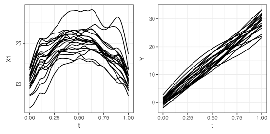
Figure 1: Plot of 20 simulated observations from the reference data set of the first functional covariates and the functional response.

3.3 Control charts for multivariate functional data

In this section we show how to use the funcharts package to build control charts in the setting described in Section 2.2 with the simulated data. Note that in the second group of Phase II data, the third functional variable has a moderate mean shift of type A with severity $d=20$, while in the third group of Phase II data the third functional variable has a more severe mean shift of type A with severity $d=40$.

For class mfd, the funcharts package provides the pca_mfd() function to perform MFPCA, which is a wrapper to pca.fd() from the fda package. Note that pca_mfd() is called internally by the functions control_charts_pca(), sof_pc(), and fof_pc(), that will be shown in the next sections, before building the corresponding control charts. The funcharts provides also the plot_pca_mfd() function to plot the eigenfunctions selected by where the argument harm. For example, in Figure 2 we plot the first two eigenfunctions of the covariance operator of the three functional covariates, calculated on the reference data set observations in the object mfdI.

R> pca <- pca_mfd(mfdI[, c("X1", "X2", "X3")]) R> plot_pca_mfd(pca, harm = 1:2)

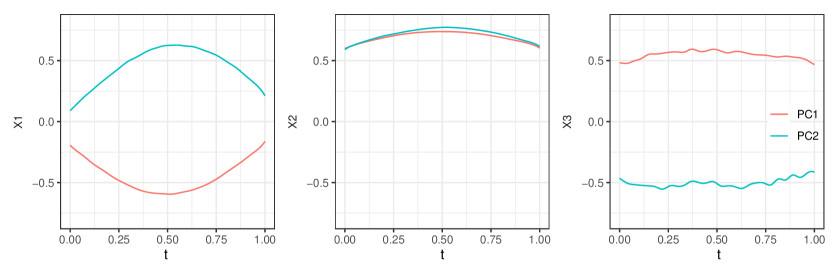
Figure 2: Plot of the first two eigenfunctions (PC1 and PC2) $\bm{\psi}_{1}(t)=(\psi_{11}(t),\psi_{12}(t),\psi_{13}(t))^{\top}$ and $\bm{\psi}_{2}(t)=(\psi_{21}(t),\psi_{22}(t),\psi_{23}(t))^{\top}$ of the empirical covariance operator of the three functional covariates X1, X2 and X3, reported in each of the three panels, respectively.

At this stage, the funcharts package can be suitably used to get a data frame with all the information required to plot the Phase II Hotelling’s $T^{2}$ and $SPE$ control charts as explained in Section 2.2.

The main arguments of control_charts_pca() are:

• pca, the fitted MFPCA model obtained as output of pca_mfd() on the reference data set.

• components, a vector of the eigenfunctions to be retained in the MFPCA model.

• tuning_data, an optional data set of IC observations to be used for control charts limits estimation. If no argument is provided, limits will be calculated as quantiles of the statistics computed on the reference data set.

• newdata, the mfd object containing the simulated observations to be monitored in Phase II.

• alpha, a numeric list containing the Type I errors to be used to estimate the Hotelling’s $T^{2}$ and $SPE$ control chart limits. The default value is list(T2 = 0.025, spe = 0.025), which uses the Bonferroni correction to ensure that the overall Type I error $\alpha$ is not larger than $0.05$.

Then, the plot_control_charts() function can be used with the data frame obtained to plot the three control charts shown in Figure 3. In the following, we select the first components that explain at least 95% of the total variability in the data, as the default option. We add two vertical dashed lines to distinguish three groups of 20 Phase II data, generated under different scenarios. Note that plot_control_charts() relies on the patchwork package (pedersen2020patchwork) to arrange the ggplot objects, and to add a vertical line to all plots through the operator &, as follows

R> cclist_pca <- control_charts_pca( + pca = pca, + tuning_data = mfdI_tun[, c("X1", "X2", "X3")], + newdata = mfdII_pca) R> plot_control_charts(cclist_pca) & + geom_vline(aes(xintercept = c(20.5)), lty = 2) + geom_vline(aes(xintercept = c(40.5)), lty = 2)

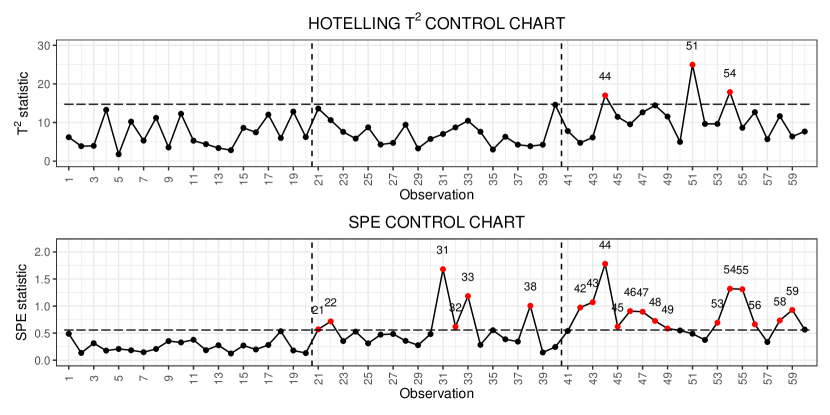
Figure 3: Control charts for multivariate functional data without covariates. Vertical lines separate the three groups of simulated Phase II data, generated as described in Section 3.1. Horizontal lines correspond to control chart limits, points correspond to the observations of the monitoring statistics for each Phase II observation. Red points highlights monitoring statistics that are out of the corresponding control limits; above each of them is reported the corresponding OC observation index.

From Figure 3, we see that the first group of 20 Phase II observations, which have been generated from the IC distribution rightly do not show up as OC points. Whereas, the second group of 20 Phase II observations, where a mean shift on the third functional variable was simulated contains OC points. Ultimately, the last group of 20 Phase II observations, where a more severe shift on the third functional variable was set, shows up as OC, except for 3 points. The funcharts package allows one to investigate also which original variable contributes the most and so may be responsible of any OC signal, through the cont_plot() function, which displays signal contributions to the Hotelling’s $T^{2}$ and $SPE$ monitoring statistics. For example, let us consider observation 59, which is OC in the $SPE$ control chart. The main arguments of cont_plot() are:

• cclist, the data frame returned by control_charts_sof_pc.

• id_num, the index of the observation whose contributions are to be plotted.

• which_plot, a vector containing the desired contribution to be plotted, where "T2" denotes the Hotelling’s $T^{2}$ statistic and "spe" denotes the $SPE$ statistic.

The contributions are shown as bar plots, where upper control limits are added as lines estimated on the Phase I tuning data. Contributions that exceed the limits are plotted in red color otherwise bar are plotted in gray. The contributions in Figure 4 show the second and third functional variables as the main responsible of the OC in the $SPE$ statistic, thus correctly signaling the simulated mean shift. Note that, even though we simulated a mean shift in varaible $X_{3}$, contribution of the functional variable $X_{2}$ is also particularly large. This is reasonable because variable $X_{3}$ affects the entire covariance structure in the data, which can turn into large contributions to the monitoring statistics also from other variables correlated with it.

R> cont_plot(cclist = cclist_pca, id_num = 59, which_plot = "spe")

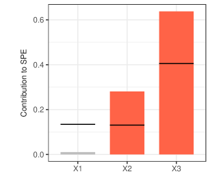
Figure 4: Contribution of the functional covariates to the Hotelling’s $SPE$ statistic for the Phase II observation 59. Contributions exceeding upper control limits depicted by horizontal lines are plotted in red.

Finally, we can also plot any future observation against the reference data set by using the plot_mon() function, as shown in Figure 5. Its main arguments are:

• cclist, the data frame returned by control_charts_pca.

• fd_train, an mfd object containing the data set to be plotted in the background in gray. Usually the reference data set of functional variables representing the IC performance is provided.

• fd_test, an mfd object containing the data to be monitored in Phase II and plotted on the foreground. Functions whose contribution to either the Hotelling’s $T^{2}$ and $SPE$ statistics is out of control are plotted in red.

R> plot_mon(cclist = cclist_pca, + fd_train = mfdI[, c("X1", "X2", "X3")], + fd_test = mfdII_pca[59])

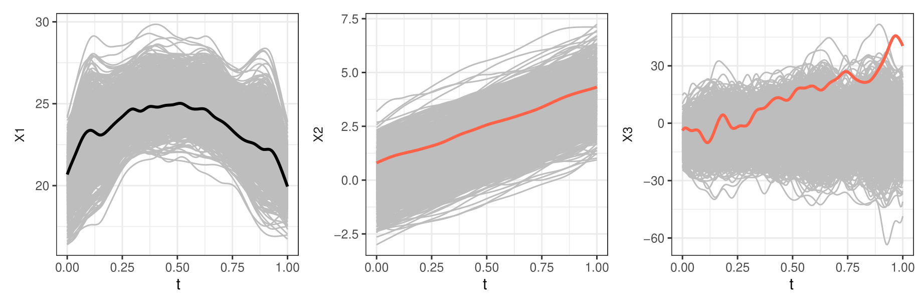
Figure 5: Observation 59 of the functional covariates in the Phase II data set, plotted against the observations of the reference data set used for model fitting, plotted in gray. Red curves correspond to functional variables whose contribution to at least one monitoring statistic exceeds its limit, while the other curves are plotted as black lines.

3.4 Functional control charts for a univariate quality characteristic adjusted by the influence of covariates

The use of the funcharts package to implement functional control charts for a univariate quality characteristic adjusted by the influence of covariates is illustrated in Sections 3.4.1 and 3.4.2 with reference to scalar-on-function and function-on-function regression cases, respectively introduced in Sections 2.3.1 and 2.3.2.

3.4.1 Control charts based on scalar-on-function regression

To fit a scalar-on-function regression model with the reference data set, the funcharts package provides the sof_pc() function. Its main arguments are:

• y, the vector containing the scalar response variable observations.

• mfdobj_x, an mfd object containing the observations of the functional covariates.

• tot_variance_explained, the minimum desired fraction of variance to be explained by the set of PCs retained into the MFPCA model fitted on the functional covariates. Default value is 0.9.

• selection, the criterion to choose the PCs to retain as predictors in regression model. "variance" (default) retains the first $M$ PCs such that together they explain a fraction of variance greater than tot_variance_explained, "PRESS" selects the $j$-th functional PC if, by adding it to the current set of selected PCs, the predicted residual error sum of squares (PRESS) statistic decreases. "gcv" is similar to "PRESS", where the PRESS statistic is substituted by the GCV score.

The following code uses default arguments and estimates the scalar-on-function regression model with the reference data set:

R> mod_sof <- sof_pc(y=d$datI$y_scalar, mfdobj_x=mfdI[,c("X1","X2","X3")])

The output of sof_pc is a list including the results of the regression of the scalar response on the scores, the results of the MFPCA obtained using pca_mfd() and the estimated functional regression coefficient, as an object of class mfd. The latter can be plotted using the plot_mfd() function. Moreover, the funcharts package allows the graphical uncertainty quantification of the functional coefficient estimates via the plot_bootstrap_sof_pc() function, which plots the coefficients estimated on the reference data set along with estimates obtained on bootstrap samples of the same data set, as in Figure 6:

R> plot_bootstrap_sof_pc(mod_sof, nboot = 100)

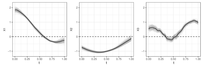
Figure 6: Estimated functional coefficients of the scalar-on-function regression model on the simulated reference data set, plotted in black, along with estimates of functional coefficients on 10 bootstrap samples, plotted in gray, for uncertainty quantification.

Once the model has been estimated on the reference data set, it is possible to build the control charts and plot them for the prospective monitoring of the process, given the new Phase II data set. As stated in Section 3.1, the first group of data contains IC observations, in the second group of data, the scalar response has a moderate mean ($d=1$), while in the third group of data, the scalar response has a more severe mean shift ($d=2$). Mean shifts of covariates are the same as in Section 3.3. As explained in Section 2.3.1, capezza2020control propose three control charts based on the Hotelling’s $T^{2}$ and SPE to monitor the multivariate functional covariates, together with the prediction error on the scalar response variable to monitor the scalar response variable, conditionally on the covariates. The control_charts_sof_pc() function provides a data frame with all the information required to plot the desired control charts. It has the following main arguments:

• mod, the fitted model obtained as output of sof_pc.

• mfdobj_x_tuning, an optional data set of IC observations of the functional covariates to be used for control charts tuning. If no argument is provided, limits will be calculated as quantiles of the statistics computed on the reference data set.

• y_test, the vector containing the observations of the scalar response variable to be monitored in Phase II.

• mfdobj_x_test, the mfd object containing the observations of the multivariate functional covariates, corresponding to y_test.

• alpha, a list containing the Type I error for each control chart. The default value is list(T2 = 0.0125, spe = 0.0125, y = 0.025), which uses the Bonferroni correction to ensure that the overall Type I error $\alpha$ is not larger than $0.05$.

The plot_control_charts() function can be used with the obtained data frame to plot the three control charts as shown in Figure 7.

R> cclist_sof_pc <- control_charts_sof_pc( + mod = mod_sof, + mfdobj_x_tuning = mfdI_tun[, c("X1", "X2", "X3")], + y_test = d$datII_{s}of$y_scalar, + mfdobj_x_test = mfdII[, c("X1", "X2", "X3")]) R> plot_control_charts(cclist_sof_pc) & + geom_vline(aes(xintercept = c(20.5)), lty = 2) + geom_vline(aes(xintercept = c(40.5)), lty = 2)

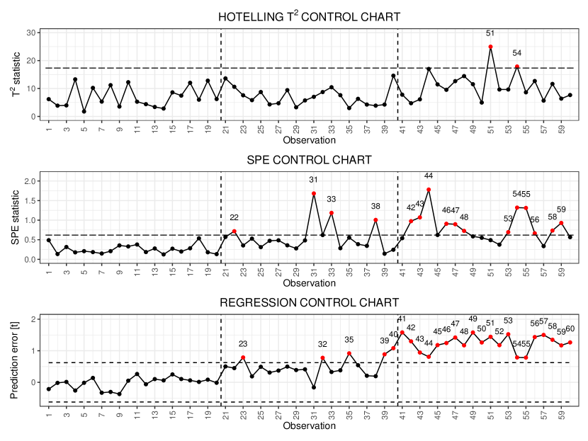
Figure 7: Functional control charts for the scalar-on-function regression case. Vertical lines separate the three groups of simulated Phase II data. Horizontal lines correspond to control chart limits, points correspond to the observations of the monitoring statistics for each Phase II observation. Red points highlights monitoring statistics that are out of the corresponding control limits; above each of them is reported the corresponding OC observation index.

Since the multivariate functional covariates observations are the same as the data used in Section 3.3, by comparing Figures 7 and 3, notice that the Hotelling’s $T^{2}$ and $SPE$ control charts plot the same values of the monitoring statistics. The control_charts_sof_pc() function calls in fact control_charts_pca() on the multivariate functional covariates. Control limits in Figure 7 are higher than those of Figure 3 because the Bonferroni correction takes into account the use of three control charts instead of two. The third control chart (for the scalar prediction error monitoring) signals 5 OC alarms over the second group of 20 data, while all 20 observations in the third group are above the upper control limit. When an OC alarm is signaled by the Hotelling’s $T^{2}$ or $SPE$ control charts, one can build contribution plots on the multivariate functional covariates as shown in Section 3.3 and further visualize any multivariate functional observation against a reference data set to perform fault detection on multivariate functional covariates. When instead the response prediction error control chart issues an OC alarm, while the Hotelling’s $T^{2}$ and $SPE$ charts do not, one concludes that possible anomalies may have occurred outside of the set of variables chosen as functional covariates.

3.4.2 Control charts based on function-on-function regression

To fit a function-on-function regression model with a reference data set, the funcharts package provides the fof_pc() function, having arguments

• mfdobj_y and mfdobj_x, the mfd objects with the Phase I observations of the functional response and covariates, respectively.

• tot_variance_explained_x, tot_variance_explained_y and tot_variance_explained_res, the minimum fraction of variance that have to be explained by the set of PCs retained into the MFPCA model fitted on the functional covariates, response and residuals, respectively. Default value is 0.95.

• type_residuals, the functional residual to be monitored (see choice (iii) of centofanti2020functional). If "standard" (default), the MFPCA is calculated on the functional residuals. If "studentized", the MFPCA is calculated on the studentized residuals.

The following code uses default arguments and estimates the function-on-function regression model with the reference data set:

R> mod_fof <- fof_pc(mfdobj_y = mfdI[, "Y"], + mfdobj_x = mfdI[, c("X1", "X2", "X3")])

As output, fof_pc returns a list including the results of the regression of the functional response scores on the functional covariate scores, the results of the MFPCA obtained using pca_mfd() on the functional response, the functional covariates and residuals. Moreover, the output list contains the estimated regression coefficient function, as an object of class bifd from the fda package. Thus, it can be plotted via the plot_bifd() function provided by the funcharts package, as in Figure 8.

R> plot_bifd(mod_fof$beta_{f}d)\begin{figure}\par{\centering\includegraphics[width=433.62pt]{fig/beta_fof.pdf}\par\@add@centering}\par\@@toccaption{{\lx@tag[ ]{{8}}{Plotofthethefunction-on-functionregressioncoefficientestimatedonthesimulatedreferencedataset.}}}\@@caption{{\lx@tag[: ]{{Figure 8}}{Plotofthethefunction-on-functionregressioncoefficientestimatedonthesimulatedreferencedataset.}}}\end{figure}\par\par Oncethemodelhasbeenestimatedonthereferencedataset,itispossibletobuildthecontrolchartsfortheprospectivemonitoringoftheprocess,giventhenewPhaseIIdataset.AsstatedinSection\ref{how_to_simulate},thefirstgroupofdatacontainsICobservations,whereas,inthesecondandthirdgroupsofdata,thefunctionalresponsehasamoderatemeanshiftoftypeDwithseverity$d=0.5$and$d=1.5$,respectively.TheconsideredmeanshiftsofcovariatesarethesameasinSection\ref{sec_using_colosimo}.AsexplainedinSection\ref{sec_methods_centofanti},twocontrolchartsareusedforSPMinthiscase,basedontheHotelling^{\prime}s$T^{2}$andthesquaredpredictionerrormonitoringstatistics,calculatedonthefunctionalresidualsofthefunction-on-functionregressionmodel.The\texttt{regr\_cc\_fof()}functionprovidesadataframewithalltheinformationrequiredtoplotthecontrolchart.Ithasthefollowingmainarguments:\par\begin{itemize} \par\itemize@item@{object}, the fitted model obtained as output of {fof\_pc}. \par\itemize@item@{mfdobj\_y\_tuning} and {mfdobj\_x\_tuning}, optional {mfd} objects of reference observations of the functional response and covariates, respectively, to be used for control chart tuning. If no argument is provided, limits will be calculated as quantiles of the statistics computed on the reference data set. \par\itemize@item@{mfdobj\_y\_new} and {mfdobj\_x\_new}, the {mfd} objects with the observations to be monitored in Phase II of the functional response and covariates, respectively. \par\itemize@item@{alpha}, the list containing the Type I error for the Hotelling's $T^{2}$ and the $SPE$ control charts. The default value is {list(T2\ =\ 0.025,\ spe\ =\ 0.025)}, which uses the Bonferroni correction to ensure the overall Type I error $\alpha$ is not larger than $0.05$. \par\end{itemize}\par The\texttt{plot\_control\_charts()}functioncanbeusedtoplotthecontrolchartsasinFigure\ref{fig:fof_cc}.\par\CodeChunk\CodeInput R>cclist_{f}of_{p}c<-regr_{c}c_{f}of(+object=mod_{f}of,+mfdobj_{y}{}_{t}uning=mfdI_{t}un[,"Y"],+mfdobj_{x}{}_{t}uning=mfdI_{t}un[,c("X1","X2","X3")],+mfdobj_{y}{}_{n}ew=mfdII_{f}of[,"Y"],+mfdobj_{x}{}_{n}ew=mfdII_{f}of[,c("X1","X2","X3")])R>plot_{c}ontrol_{c}harts(cclist_{f}of_{p}c)&+geom_{v}line(aes(xintercept=c(20.5)),lty=2)+geom_{v}line(aes(xintercept=c(40.5)),lty=2)\begin{figure}\par{\centering\includegraphics[width=433.62pt]{fig/cc_fof.pdf}\par\@add@centering}\par\@@toccaption{{\lx@tag[ ]{{9}}{PhaseIIcontrolchartingforthefunction-on-functionregressioncase.VerticallinesseparatethethreegroupsofsimulatedPhaseIIdata.Horizontallinescorrespondtocontrolchartlimits,pointscorrespondtotheobservationsofthemonitoringstatisticsforeachobservation.Redpointsandobservationindexhighlightmonitoringstatisticsthatareoutofthecorrespondingcontrollimits.}}}\@@caption{{\lx@tag[: ]{{Figure 9}}{PhaseIIcontrolchartingforthefunction-on-functionregressioncase.VerticallinesseparatethethreegroupsofsimulatedPhaseIIdata.Horizontallinescorrespondtocontrolchartlimits,pointscorrespondtotheobservationsofthemonitoringstatisticsforeachobservation.Redpointsandobservationindexhighlightmonitoringstatisticsthatareoutofthecorrespondingcontrollimits.}}}\end{figure}\par Inthefirstgroupofobservations(generatedfromICprocess)thereisafalsealarmsignaledbythe$SPE$controlchart,inthesecondgroupofobservations(whicharegeneratedwithmoderatemeanshiftonboththethirdfunctionalcovariateandthefunctionalresponse),onlythreeobservationswithinthecontrollimits,whileinthelastgroup(withmoreseveremeanshifts)allobservationsaresignaledasOC.\par Notethat\texttt{regr\_cc\_fof()}providescontrolchartsonthepredictionerrorofthefunctionalresponse,withoutmonitoringdirectlythemultivariatefunctionalcovariates.Thismeansthat,forexample,anobservationwithparticularlyanomalousvaluesofsomefunctionalcovariatesthatstillproducesgoodpredictionofthefunctionalresponse,suchthatthepredictionerrorplotsIC.Thishappensbecause\cite[cite]{\@@bibref{Authors Phrase1YearPhrase2}{centofanti2020functional}{\@@citephrase{(}}{\@@citephrase{)}}}focusedonansweringtotheresearchquestion:\textit{given the value of the functional covariates, is the observed response profile as expected?}\par$

The funcharts package provides the real-time functional control charts stated in Section 2.4 through the functions control_charts_pca_mfd_real_time(), control_charts_sof_pc_real_time(), and regr_cc_fof_real_time(), which are the real-time version of the main functions presented in Section 2.2, 2.3.1 and 2.3.2, respectively. For shortness, in this section we illustrate only the real-time version of the functional control chart based on function-on-function regression introduced in Section 2.3.2 and implemented in Section 3.4.2. Starting from the functional domain $\mathcal{T}=(a,b)$, in the following, we consider the evolution of the functional data over the subintervals $(a,a+k(b-a)))$, with $k$ varying along k_seq, which is an additional input vector containing values defining the fraction of domain over which functional data are partially observed. By default, k_seq is the sequence of values 0.2, 0.3, …, 1. In the same way as the corresponding functions developed for the completely observed functional data, the funcharts package provides the functions get_mfd_array_real_time(), get_mfd_list_real_time() and get_mfd_df_real_time(), which accept as input lists of matrices, arrays and data frames in the long format. These functions return as output a list of mfd objects, each partially observed on the interval $(a,a+k(b-a)))$ and create the data sets required to perform the real-time functional control charts, as per the following code.

R> xI <- get_mfd_list_real