IBP reduction via Gröbner bases
in a rational double-shift algebra

Abstract

We report on an approach to integration-by-parts reduction based on Gröbner bases. We establish the underlying noncommutative rational double-shift algebra wherein the integration-by-parts relations form a left ideal. We describe in detail the one-loop massless box as an example where we achieved the full reduction to master integrals by means of the Gröbner basis approach, and report on the performance of the implementation. We also identify potential bottlenecks in more complicated examples and elaborate on interesting further directions.

1 Introduction

Reduction of dimensionally regularized Feynman integrals based on integration-by-parts (IBP) relations [1, 2] is an indispensable tool for carrying out higher-order calculations in perturbative quantum field theory. Many sophisticated public and private codes to perform this task exist in various programming languages, for instance ${\mathtt{AIR}}$ [3], ${\mathtt{FIRE}}$ [4, 5, 6], ${\mathtt{Reduze}}$ [7, 8], ${\mathtt{LiteRed}}$ [9], and ${\mathtt{Kira}}$ [10, 11].

The reduction procedures that have been implemented in these programs are mostly based on Laporta’s algorithm [12] which solves the IBP equations for numerical values of the propagator powers of the integral using “bottom-up” Gaussian elimination. In recent years, several refinements of this algorithm have been developed to speed up the calculation, which are mostly based on parallelization and ideas from finite fields and rational reconstruction [13, 14, 6, 15, 16, 17].

The Laporta algorithm has served the community in countless multi-loop calculations over the past two decades. It has, however, also a couple of drawbacks. For instance, in many cases redundant integrals have to be computed during the reduction procedure in order to get access to those integrals that are required by the actual calculation of physical quantities. Consequently, storing the results of typically ${\cal O}(10^{\sim 4-6})$ integrals demands for large storage capacities. Moreover, plugging in integer values for the propagator powers generates a huge system of equations, whose solution via Gaussian elimination generates a considerable expression swell at intermediate stages, at least as long as none of the aforementioned refinements are applied.

More recently, new ideas towards a more direct reduction procedure have been developed. They are mostly based on syzygy equations [18, 19, 20, 21, 22], algebraic geometry [23, 24, 25], and intersection numbers [26, 27, 28, 29, 30, 31, 32, 33]. In these proceedings we report on work in progress [34], where we choose an approach to IBP reduction that is based on Gröbner bases and hence leaves the propagator powers parametric. While IBP reductions by means of Gröbner bases have been attempted in the past [35, 36, 37, 38, 39, 40, 41, 42], we formulate for the first time the appropriate noncommutative rational double-shift algebra wherein the IBP relations generate a left ideal. For selected examples of which we describe one representative below, we were able to compute the Gröbner basis for the left ideal of IBP relations in the noncommutative rational double-shift algebra and achieved the full reduction with the Gröbner basis technique.

This article is organized as follows. In the next section we recap the basics about Gröbner bases and related terms from algebraic geometry. In section 3 we establish the noncommutative rational double-shift algebra wherein the IBP relations form a left ideal. Section 4 contains the one-loop massless box as an explicit example where we achieved a full reduction with the Gröbner basis approach. We conclude in section 5.

2 Basics about Gröbner bases

We first give the definitions of a few key quantities necessary for our calculation and its description in the subsequent sections.

Let $R$ be a ring. A left ideal $I\subseteq R$ is an additive subgroup of $R$ fulfilling

$$r\in R\wedge a\in I\;\Longrightarrow\;ra\in I.$$ (1)

As a simple example, the set of even integers forms a (left) ideal in the ring $\mathbb{Z}$ of integers.

A monomial order on the polynomial algebra $R=\mathbb{K}[x]=\mathbb{K}[x_{1},\ldots,x_{n}]$ over a field $\mathbb{K}$ is a total order $>$ such that

$$x^{\alpha}>x^{\beta}\;\Longrightarrow\;x^{\gamma}x^{\alpha}>x^{\gamma}x^{\beta}\quad\forall\,\alpha,\beta,\gamma\in\mathbb{N}^{n}\,,$$ (2)

where $\alpha$, $\beta$, and $\gamma$ are multi-indices. The most prominent (global) monomial orders are the lexicographic order for which

$$x^{\alpha}>_{\mbox{{\scriptsize{lex}}}}x^{\beta}\quad\Longleftrightarrow\quad\mbox{first nonzero entry of }\alpha-\beta>0$$ (3)

has to hold, and the degree reverse lexicographic order with condition

$$x^{\alpha}>_{\mbox{{\scriptsize{drlex}}}}x^{\beta}\Longleftrightarrow(\mbox{\footnotesize{deg} }x^{\alpha}>\mbox{\footnotesize{deg} }x^{\beta})\mbox{ or }(\mbox{\footnotesize{deg} }x^{\alpha}=\mbox{\footnotesize{deg} }x^{\beta}\mbox{ and last nonzero entry of }\alpha-\beta<0).$$ (4)

For $f\in R$, the leading term ${\boldsymbol{L}}_{>}(f)$ with respect to a given monomial order $>$ is the largest term in $f$ with respect to $>$. A finite subset $G=\{f_{1},\ldots,f_{r}\}\subset I$ is a Gröbner basis for the (left) ideal $I$ if

$${\boldsymbol{L}}_{>}(I)={\boldsymbol{L}}_{>}(G)\,,$$ (5)

i.e. the leading (left) ideal of $I$ is generated by the leading terms of the elements of $G$. Hence $G$ generates $I$. One way of computing Gröbner bases in polynomial algebras is via Buchberger’s algorithm. In this work we use a generalization of Buchberger’s algorithm to the context of Ore algebras as developed in [43]. This class includes the aforementioned polynomial algebras, but also a wide class of noncommutative algebras, including the rational double-shift algebra which is central to this work.

The remainder $h$ of $g=\sum_{i=1}^{r}\,g_{i}\,f_{i}+h$ is uniquely determined by $g$, $I$, and $>$. Moreover, we will call $\operatorname{NF}_{I,>}(g)=\operatorname{NF}_{G}(g)=h$ the normal form of $g$ mod $I$ with respect to $>$.

3 Noncommutative rational double-shift algebra

We start from a generic $L$-loop integral

$$J(a_{1},\ldots,a_{n})=\int\operatorname{d}^{D}\ell_{1}\cdots\operatorname{d}^{D}\ell_{L}\,\frac{1}{P_{1}^{a_{1}}\cdots P_{n}^{a_{n}}}\mbox{,}$$ (6)

where $D$ is the number of space-time dimensions in dimensional regularization. Each of the propagators $P_{i}$, $i=1,\ldots,n$, is usually of the form $P_{i}=m_{i}^{2}-p_{i}^{2}$ with mass $m_{i}$ and $p_{i}$ a linear combination of the $L$ loop momenta $\ell_{1},\ldots,\ell_{L}$ and $E$ external momenta $k_{1},\ldots,k_{E}$. The integral therefore depends on the propagator powers (indices) $a_{i}$, the number of space-time dimensions $D$, the masses $m_{i}^{2}$ and kinematic invariants built out of the the external momenta which we collectively label $s_{ij}$. In the following we will suppress all dependence of $J$ but that on the indices $a_{i}$.

The $L(L+E)$ standard IBP relations that are derived from

$$\int\operatorname{d}^{D}\ell_{1}\cdots\operatorname{d}^{D}\ell_{L}\;\frac{\partial}{\partial\ell_{j}^{\mu}}\left(\frac{v_{k}^{\mu}}{P_{1}^{a_{1}}\cdots P_{n}^{a_{n}}}\right) =0\,\mbox{,}$$ (7)

with $v_{k}^{\mu}$ any loop or external momentum, can be expressed in terms of shift operators $D_{i}$, $D_{i}^{-}$ and multiplication operators $a_{i}$, $i=1,\ldots,n$, with the following partial right action on the space of loop integrals $J(z_{1},\ldots,z_{n})$:

$$J(\ldots,z_{i},\ldots)\bullet D_{i} =J(\ldots,z_{i}-1,\ldots), \quad\underbrace{J(\ldots,z_{i},\ldots)}_{\text{not scaleless}}\bullet D_{i}^{-} =J(\ldots,z_{i}+1,\ldots),$$

$$J(\ldots,z_{i},\ldots)\bullet a_{i} =z_{i}J(\ldots,z_{i},\ldots), \quad J(\ldots,\underbrace{z_{i}}_{\neq 0},\ldots)\bullet a_{i}^{-1} =\frac{1}{z_{i}}J(\ldots,z_{i},\ldots)\mbox{.}$$ (8)

Our computations take place in the noncommutative rational double-shift algebra

$$Y:=\mathbb{Q}(D,s_{ij},m_{i}^{2})(a_{1},\ldots,a_{n})\langle D_{j},D_{j}^{-}\mid j=1,\ldots,n\rangle$$ (9)

in the indeterminates $a_{1},\ldots,a_{n},D_{1},\ldots,D_{n},D_{1}^{-},\ldots,D_{n}^{-}$ which satisfy the relations

$$[a_{i},D_{j}]=\delta_{ij}D_{i}\,\mbox{,}\qquad[a_{i},D_{j}^{-}]=-\delta_{ij}D_{i}^{-}\,\mbox{,}\qquad D_{i}D_{i}^{-}=1=D_{i}^{-}D_{i}\,\mbox{,}$$

$$[a_{i},a_{j}]=[D_{i},D_{j}]=[D_{i}^{-},D_{j}^{-}]=[D_{i},D_{j}^{-}]=0\,\mbox{.}$$ (10)

The standard IBP relations generate a left ideal in the noncommutative rational double-shift algebra

$$I_{\mathrm{IBP}} \coloneqq\langle r_{i}\mid i=1,\ldots,L(L+E)\rangle_{Y}\lhd Y\mbox{.}$$

Our goal will be to compute a Gröbner basis for the left ideal $I_{\mathrm{IBP}}$ in $Y$.

We close this section by defining a standard monomial with respect to the Gröbner basis $G$ of $I_{\mathrm{IBP}}$, which is a monomial $m$ in the indeterminates $D_{i},D_{j}^{-}$ such that $\operatorname{NF}_{G}(m)=m$. The set of standard monomials forms a basis for the finite-dimensional vector space $Y/I_{\mathrm{IBP}}$ over the field $\mathbb{Q}(D,s_{ij},m_{i}^{2})$ of coefficients, and corresponds to a set of master integrals with respect to some fixed initial integral, usually taken to be the corner integral of the topology under consideration.

For the technical implementation we developed the GAP package $\mathtt{LoopIntegrals}$ [44], which relies on Chyzak’s Maple package $\mathtt{Ore\_algebra}$ [43] to perform Gröbner basis computations in the noncommutative double-shift algebra with rational coefficients. The interface between GAP [45] and $\mathtt{Ore\_algebra}$ is provided by the $\mathtt{homalg}$-project packages [46].

4 One-loop massless box

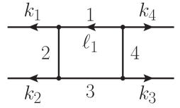
Figure 1: The Feynman graph of the one-loop box integral.

An example of a successful application of the Gröbner basis approach to IBP reduction is the one-loop massless box depicted in figure 1. It is defined by the loop momentum $\ell_{1}$ and the external momenta $k_{1},k_{2},k_{3},k_{4}$, of which we take $k_{1},k_{2},k_{4}$ to be the linearly independent ones. The external lines are on-shell and massless, i.e. $k_{i}^{2}=0$ for $i=1,2,3,4$, which results in the independent external kinematic invariants $s_{12}=2k_{1}\cdot k_{2}$ and $s_{14}=2k_{1}\cdot k_{4}$. Internal lines are also massless. The $n=4$ propagators are

$$P_{1} =-\ell_{1}^{2}\,\mbox{,} P_{2} =-(\ell_{1}-k_{1})^{2}\,\mbox{,} P_{3} =-(\ell_{1}-k_{1}-k_{2})^{2}\,\mbox{,} P_{4} =-(\ell_{1}+k_{4})^{2}\,\mbox{,}$$ (11)

from which we derive the four standard IBP relations

$$r_{1} =-a_{2}D_{1}D_{2}^{-}-a_{3}D_{1}D_{3}^{-}-a_{4}D_{1}D_{4}^{-}-s_{12}a_{3}D_{3}^{-}+(D-2a_{1}-a_{2}-a_{3}-a_{4}),$$

$$r_{2} =a_{1}D_{1}^{-}D_{2}-a_{2}D_{1}D_{2}^{-}-a_{3}D_{1}D_{3}^{-}+a_{3}D_{2}D_{3}^{-}-a_{4}D_{1}D_{4}^{-}+a_{4}D_{2}D_{4}^{-}-s_{12}a_{3}D_{3}^{-}+s_{14}a_{4}D_{4}^{-}-a_{1}+a_{2},$$

$$r_{3} =-a_{1}D_{1}^{-}D_{2}+a_{1}D_{1}^{-}D_{3}+a_{2}D_{2}^{-}D_{3}-a_{3}D_{2}D_{3}^{-}-a_{4}D_{2}D_{4}^{-}+a_{4}D_{3}D_{4}^{-}+s_{12}a_{1}D_{1}^{-}-s_{14}a_{4}D_{4}^{-}-a_{2}+a_{3},$$

$$r_{4} =a_{2}D_{1}D_{2}^{-}+a_{3}D_{1}D_{3}^{-}-a_{1}D_{1}^{-}D_{4}-a_{2}D_{2}^{-}D_{4}-a_{3}D_{3}^{-}D_{4}+a_{4}D_{1}D_{4}^{-}-s_{14}a_{2}D_{2}^{-}+s_{12}a_{3}D_{3}^{-}+a_{1}-a_{4}\mbox{.}$$ (12)

By means of the techniques described in the previous sections, we compute the reduced Gröbner basis $G$ in the noncommutative rational double-shift algebra

$$Y=\mathbb{K}(a_{1},a_{2},a_{3},a_{4})\langle D_{i},D_{i}^{-}\mid i=1,\ldots,4\rangle\,\mbox{.}$$ (13)

over the field $\mathbb{K}=\mathbb{Q}(D,s_{12},s_{14})$ of coefficients. It has the 9 elements

$$\allowdisplaybreaks G =\bigg{\{}D_{4}-D_{2}+\frac{(a_{2}-a_{4})s_{14}}{D-a_{1234}},D_{3}-D_{1}+\frac{(a_{1}-a_{3})s_{12}}{D-a_{1234}},$$

$$4(a_{2}-1)(D-a_{1234})D_{3}-2(D-2a_{134})(D-a_{1234})D_{4}+(D-2a_{14}-2)(D-2a_{234})s_{12}$$

$$-2(D-2a_{134})(a_{2}-a_{4})s_{14}-\frac{(D-2a_{14}-2)(D-2a_{34}-2)a_{4}s_{12}s_{14}}{D-a_{1234}-1}\,D_{4}^{-},$$

$$-2(D-2a_{234})(D-a_{1234})D_{3}+4(a_{1}-1)(D-a_{1234})D_{4}-2(a_{1}-a_{3})(D-2a_{234})s_{12}$$

$$+(D-2a_{23}-2)(D-2a_{134})s_{14}-\frac{(D-2a_{23}-2)a_{3}(D-2a_{34}-2)s_{12}s_{14}}{D-a_{1234}-1}\,D_{3}^{-},$$

$$4(D-a_{1234})(a_{4}-1)D_{3}-2(D-2a_{123})(D-a_{1234})D_{4}$$

$$+(D-2a_{12}-2)(D-2a_{234})s_{12}-\frac{(D-2a_{12}-2)a_{2}(D-2a_{23}-2)s_{12}s_{14}}{D-a_{1234}-1}\,D_{2}^{-},$$

$$-2(D-2a_{124})(D-a_{1234})D_{3}+4(a_{3}-1)(D-a_{1234})D_{4}$$

$$+(D-2a_{12}-2)(D-2a_{134})s_{14}-\frac{a_{1}(D-2a_{12}-2)(D-2a_{14}-2)s_{12}s_{14}}{D-a_{1234}-1}\,D_{1}^{-},$$

$$-2(D-2a_{1234}+4)(D-a_{1234}+1)D_{4}^{2}+(D-2a_{124}+2)(D-2a_{234}+2)s_{12}D_{4}$$

$$-2(D-2a_{1234}+4)(a_{2}-a_{4}+1)s_{14}D_{4}+4(a_{2}-1)(a_{4}-1)s_{14}D_{3}$$

$$-\frac{(D-2a_{124}+2)(D-2a_{34})(a_{4}-1)s_{12}s_{14}}{D-a_{1234}},$$

$$-(D-2a_{1234}+4)(D-a_{1234}+1)D_{3}D_{4}+(a_{3}-1)(D-2a_{234}+2)s_{12}D_{4}$$

$$+(D-2a_{134}+2)(a_{4}-1)s_{14}D_{3}-\frac{(a_{3}-1)(D-2a_{34})(a_{4}-1)s_{12}s_{14}}{D-a_{1234}},$$

$$-2(D-2a_{1234}+4)(D-a_{1234}+1)D_{3}^{2}+(D-2a_{123}+2)(D-2a_{134}+2)s_{14}D_{3}$$

$$-2(a_{1}-a_{3}+1)(D-2a_{1234}+4)s_{12}D_{3}+4(a_{1}-1)(a_{3}-1)s_{12}D_{4}$$

$$-\frac{(D-2a_{123}+2)(a_{3}-1)(D-2a_{34})s_{12}s_{14}}{D-a_{1234}}\bigg{\}}\mbox{,}$$ (14)

with the abbreviations $a_{i_{1}\ldots i_{k}}\coloneqq\sum_{j=1}^{k}a_{i_{j}}$. The Gröbner basis $G$ is rational in $D$, $a_{i}$, $s_{ij}$, and polynomial in $D_{i}$ and $D_{i}^{-}$, as expected.

We can now compute the normal forms of the indeterminates $D_{i}$, which reveal the $V_{4}$-symmetry of the problem,

$$\operatorname{NF}_{G}(D_{1})= D_{3}+\frac{(a_{1}-a_{3})s_{12}}{D-a_{1234}}\,, \operatorname{NF}_{G}(D_{3})= D_{3}\,,$$

$$\operatorname{NF}_{G}(D_{2})= D_{4}+\frac{(a_{2}-a_{4})s_{14}}{D-a_{1234}}\,, \operatorname{NF}_{G}(D_{4})= D_{4}\,.$$ (15)

The set of standard monomials with respect to $G$ is therefore $\{1,D_{3},D_{4}\}$, which correspond to the three master integrals

$$\{J(1,1,1,1),J(1,1,0,1),J(1,1,1,0)\}\mbox{,}$$ (16)

i.e. the Gröbner basis reduction yields the box and two triangles as basis of master integrals. Computing further the normal forms of the monomials $D_{1}D_{2}$, $D_{1}D_{4}$, $D_{2}D_{3}$, $D_{3}D_{4}$ with respect to the Gröbner basis $G$, one can easily verify that they are scaleless with respect to $J(1,1,1,1)$. Based on this and other examples we conjecture that the Gröbner basis reduction recognizes the scaleless integrals of a given topology.

We proceed by computing the normal form of the operators $a_{i}D_{i}^{-}$ with respect to the Gröbner basis $G$ of the left ideal $I_{\mathrm{IBP}}=\langle r_{i}\mid i=1,\ldots,4\rangle_{Y}\lhd Y$ generated by the standard IBP relations in eq. (12),

$$\allowdisplaybreaks\operatorname{NF}_{G}(a_{1}D_{1}^{-})= -\frac{2\left(D-2a_{124}\right)\!\left(D-a_{1234}\right)\!\left(D-a_{1234}-1\right)}{\left(D-2a_{12}-2\right)\left(D-2a_{14}-2\right)s_{12}s_{14}}D_{3}+\frac{4\left(a_{3}-1\right)\!\left(D-a_{1234}\right)\!\left(D-a_{1234}-1\right)}{\left(D-2a_{12}-2\right)\left(D-2a_{14}-2\right)s_{12}s_{14}}D_{4}$$

$$+\frac{\left(D-2a_{134}\right)\left(D-a_{1234}-1\right)}{\left(D-2a_{14}-2\right)s_{12}},$$

$$\operatorname{NF}_{G}(a_{2}D_{2}^{-})= \frac{4\left(a_{4}-1\right)\left(D-a_{1234}\right)\left(D-a_{1234}-1\right)}{\left(D-2a_{12}-2\right)\left(D-2a_{23}-2\right)s_{12}s_{14}}D_{3}-\frac{2\left(D-2a_{123}\right)\left(D-a_{1234}\right)\left(D-a_{1234}-1\right)}{\left(D-2a_{12}-2\right)\left(D-2a_{23}-2\right)s_{12}s_{14}}D_{4}$$

$$+\frac{\left(D-2a_{234}\right)\left(D-a_{1234}-1\right)}{\left(D-2a_{23}-2\right)s_{14}},$$

$$\operatorname{NF}_{G}(a_{3}D_{3}^{-})= -\frac{2\left(D-2a_{234}\right)\!\left(D-a_{1234}\right)\!\left(D-a_{1234}-1\right)}{\left(D-2a_{23}-2\right)\left(D-2a_{34}-2\right)s_{12}s_{14}}D_{3}+\frac{4\left(a_{1}-1\right)\!\left(D-a_{1234}\right)\!\left(D-a_{1234}-1\right)}{\left(D-2a_{23}-2\right)\left(D-2a_{34}-2\right)s_{12}s_{14}}D_{4}$$

$$+\frac{\left(D-2a_{134}\right)\left(D-a_{1234}-1\right)}{\left(D-2a_{34}-2\right)s_{12}}-\frac{2\left(a_{1}-a_{3}\right)\left(D-2a_{234}\right)\left(D-a_{1234}-1\right)}{\left(D-2a_{23}-2\right)\left(D-2a_{34}-2\right)s_{14}},$$

$$\operatorname{NF}_{G}(a_{4}D_{4}^{-})= \frac{4\left(a_{2}-1\right)\left(D-a_{1234}\right)\left(D-a_{1234}-1\right)}{\left(D-2a_{14}-2\right)\left(D-2a_{34}-2\right)s_{12}s_{14}}D_{3}-\frac{2\left(D-2a_{134}\right)\left(D-a_{1234}\right)\left(D-a_{1234}-1\right)}{\left(D-2a_{14}-2\right)\left(D-2a_{34}-2\right)s_{12}s_{14}}D_{4}$$

$$+\frac{\left(D-2a_{234}\right)\left(D-a_{1234}-1\right)}{\left(D-2a_{34}-2\right)s_{14}}-\frac{2\left(a_{2}-a_{4}\right)\left(D-2a_{134}\right)\left(D-a_{1234}-1\right)}{\left(D-2a_{14}-2\right)\left(D-2a_{34}-2\right)s_{12}}\mbox{.}$$ (17)

All $\operatorname{NF}_{G}(D_{i})$ and $\operatorname{NF}_{G}(a_{i}D_{i}^{-})$ are $\mathbb{K}$-linear combinations of the standard monomials, which leads us to conjecture that the Gröbner basis reduction also recognizes the symmetries of a problem. Moreover, we observe that in both equations (15) and (17) no nonconstant polynomials in $\mathbb{Q}[a_{1},\ldots,a_{4}]$ appear in the denominator, which means that these denominator factors in $\mathbb{K}[a_{1},\ldots,a_{4}]$ never vanish within dimensional regularization.

We conclude this section by some information on runtimes for various parts of the calculation. The Gröbner basis in eq. (14) was computed in less than 5 seconds on a modern laptop. We also implemented the computation of normal forms modulo $G$ in a FORM [47] code which we will provide electronically with [34]. The FORM program is able to do fast reductions, even for rather large values of the indices. For instance, it expresses $J(10,10,10,10)$ in terms of master integrals in less than 10 seconds on a desktop computer. However, we also mention that for problems that look at first glance only slightly more complicated than the one-loop massless box, we observe an extraordinary swell in runtime and memory consumption when attempting to compute a Gröbner basis. We will give more details on this circumstance in the next section.

5 Conclusion and outlook

We reported on recent progress in the Gröbner basis approach to IBP reduction. A key step towards a successful reduction of nontrivial Feynman integrals was to recognize that for our setup the noncommutative rational double-shift algebra is the proper algebra wherein the IBP relations generate a left ideal. The computations are organized by means of the GAP package $\mathtt{LoopIntegrals}$, which relies on the noncommutative Gröbner basis algorithms provided by Chyzak’s Maple package $\mathtt{Ore\_algebra}$.

We elaborated in detail on the one-loop massless box, for which we achieved a full reduction to master integrals within very short runtimes. This example also shows a number of appealing features of the Gröbner basis approach to IBP reduction. First, with the Gröbner basis at hand, the entire information required for reduction is available for any values of the propagator powers, which entails that no new bottom-up reduction is required if one seeks for the reduction of new or additional integrals of the same family. A second important feature that we observed in the example of the one-loop massless box is the recognition of symmetries and scaleless sectors of an integral family, which we conjecture to happen also for other, more complicated topologies.

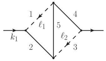
Figure 2: The Feynman graph for the kite integral. Dashed lines denote massless propagators and solid lines denote massive propagators of mass $m$. The on-shell condition implies $k_{1}^{2}=m^{2}$.

However, as so often, there is no free lunch, and hence, as the complexity of the problem increases, the Gröbner basis technique also reveals bottlenecks which potentially eat up parts of the virtues identified above. Let’s consider, for instance, the two-loop on-shell kite integral whose diagram is shown in figure 2. Compared to the one-loop massless box it has an extra loop but only a single scale. One might therefore expect the complexity of the kite to be moderately above that of the box. However, the computation of the Gröbner basis results in an extraordinary expression swell which as of now prevented us from finishing the computation. Still, we were able to compute the normal forms $\operatorname{NF}(a_{i}D_{i}^{-})$, $i=1,\ldots,5$ using a linear algebra ansatz [34], which allows, e.g., for the reduction of the top-level sector.

To conclude, the Gröbner basis technique is a viable approach to IBP reduction, of which potentially also synergies with existing implementations can be identified in the future. However, new conceptual ideas are needed to deal with the enormous intermediate expression swell with increasing complexity of reduction problems.

References

- [1] F.V. Tkachov, A Theorem on Analytical Calculability of Four Loop Renormalization Group Functions, Phys. Lett. B 100 (1981) 65.
- [2] K.G. Chetyrkin and F.V. Tkachov, Integration by Parts: The Algorithm to Calculate beta Functions in 4 Loops, Nucl. Phys. B 192 (1981) 159.
- [3] C. Anastasiou and A. Lazopoulos, Automatic integral reduction for higher order perturbative calculations, JHEP 07 (2004) 046 [hep-ph/0404258].
- [4] A.V. Smirnov, Algorithm FIRE – Feynman Integral REduction, JHEP 10 (2008) 107 [0807.3243].
- [5] A.V. Smirnov, FIRE5: a C++ implementation of Feynman Integral REduction, Comput. Phys. Commun. 189 (2015) 182 [1408.2372].
- [6] A.V. Smirnov and F.S. Chuharev, FIRE6: Feynman Integral REduction with Modular Arithmetic, Comput. Phys. Commun. 247 (2020) 106877 [1901.07808].
- [7] C. Studerus, Reduze-Feynman Integral Reduction in C++, Comput. Phys. Commun. 181 (2010) 1293 [0912.2546].
- [8] A. von Manteuffel and C. Studerus, Reduze 2 - Distributed Feynman Integral Reduction, 1201.4330.
- [9] R.N. Lee, Presenting LiteRed: a tool for the Loop InTEgrals REDuction, 1212.2685.
- [10] P. Maierhöfer, J. Usovitsch and P. Uwer, Kira—A Feynman integral reduction program, Comput. Phys. Commun. 230 (2018) 99 [1705.05610].
- [11] J. Klappert, F. Lange, P. Maierhöfer and J. Usovitsch, Integral reduction with Kira 2.0 and finite field methods, Comput. Phys. Commun. 266 (2021) 108024 [2008.06494].
- [12] S. Laporta, High precision calculation of multiloop Feynman integrals by difference equations, Int. J. Mod. Phys. A 15 (2000) 5087 [hep-ph/0102033].
- [13] A. von Manteuffel and R.M. Schabinger, A novel approach to integration by parts reduction, Phys. Lett. B 744 (2015) 101 [1406.4513].
- [14] T. Peraro, Scattering amplitudes over finite fields and multivariate functional reconstruction, JHEP 12 (2016) 030 [1608.01902].
- [15] T. Peraro, FiniteFlow: multivariate functional reconstruction using finite fields and dataflow graphs, JHEP 07 (2019) 031 [1905.08019].
- [16] J. Klappert and F. Lange, Reconstructing rational functions with FireFly, Comput. Phys. Commun. 247 (2020) 106951 [1904.00009].
- [17] J. Klappert, S.Y. Klein and F. Lange, Interpolation of dense and sparse rational functions and other improvements in FireFly, Comput. Phys. Commun. 264 (2021) 107968 [2004.01463].
- [18] J. Gluza, K. Kajda and D.A. Kosower, Towards a Basis for Planar Two-Loop Integrals, Phys. Rev. D 83 (2011) 045012 [1009.0472].
- [19] R.M. Schabinger, A New Algorithm For The Generation Of Unitarity-Compatible Integration By Parts Relations, JHEP 01 (2012) 077 [1111.4220].
- [20] R.N. Lee, Modern techniques of multiloop calculations, in 49th Rencontres de Moriond on QCD and High Energy Interactions, pp. 297–300, 2014 [1405.5616].
- [21] J. Böhm, A. Georgoudis, K.J. Larsen, M. Schulze and Y. Zhang, Complete sets of logarithmic vector fields for integration-by-parts identities of Feynman integrals, Phys. Rev. D 98 (2018) 025023 [1712.09737].
- [22] D.A. Kosower, Direct Solution of Integration-by-Parts Systems, Phys. Rev. D 98 (2018) 025008 [1804.00131].
- [23] K.J. Larsen and Y. Zhang, Integration-by-parts reductions from unitarity cuts and algebraic geometry, Phys. Rev. D 93 (2016) 041701 [1511.01071].
- [24] J. Böhm, A. Georgoudis, K.J. Larsen, H. Schönemann and Y. Zhang, Complete integration-by-parts reductions of the non-planar hexagon-box via module intersections, JHEP 09 (2018) 024 [1805.01873].
- [25] D. Bendle, J. Böhm, W. Decker, A. Georgoudis, F.-J. Pfreundt, M. Rahn et al., Integration-by-parts reductions of Feynman integrals using Singular and GPI-Space, JHEP 02 (2020) 079 [1908.04301].
- [26] P. Mastrolia and S. Mizera, Feynman Integrals and Intersection Theory, JHEP 02 (2019) 139 [1810.03818].
- [27] H. Frellesvig, F. Gasparotto, M.K. Mandal, P. Mastrolia, L. Mattiazzi and S. Mizera, Vector Space of Feynman Integrals and Multivariate Intersection Numbers, Phys. Rev. Lett. 123 (2019) 201602 [1907.02000].
- [28] H. Frellesvig, F. Gasparotto, S. Laporta, M.K. Mandal, P. Mastrolia, L. Mattiazzi et al., Decomposition of Feynman Integrals on the Maximal Cut by Intersection Numbers, JHEP 05 (2019) 153 [1901.11510].
- [29] S. Abreu, R. Britto, C. Duhr, E. Gardi and J. Matthew, From positive geometries to a coaction on hypergeometric functions, JHEP 02 (2020) 122 [1910.08358].
- [30] S. Weinzierl, On the computation of intersection numbers for twisted cocycles, J. Math. Phys. 62 (2021) 072301 [2002.01930].
- [31] S. Caron-Huot and A. Pokraka, Duals of Feynman Integrals. Part II. Generalized unitarity, JHEP 04 (2022) 078 [2112.00055].
- [32] J. Chen, X. Jiang, C. Ma, X. Xu and L.L. Yang, Baikov representations, intersection theory, and canonical Feynman integrals, 2202.08127.
- [33] V. Chestnov, F. Gasparotto, M.K. Mandal, P. Mastrolia, S.J. Matsubara-Heo, H.J. Munch et al., Macaulay Matrix for Feynman Integrals: Linear Relations and Intersection Numbers, 2204.12983.
- [34] M. Barakat, R. Brüser, C. Fieker, T. Huber and J. Piclum, Feynman integral reduction using Gröbner bases, in preparation (2022) .
- [35] O.V. Tarasov, Reduction of Feynman graph amplitudes to a minimal set of basic integrals, Acta Phys. Polon. B 29 (1998) 2655 [hep-ph/9812250].
- [36] O.V. Tarasov, Computation of Gröbner bases for two loop propagator type integrals, Nucl. Instrum. Meth. A 534 (2004) 293 [hep-ph/0403253].
- [37] V.P. Gerdt, Gröbner bases in perturbative calculations, Nucl. Phys. B Proc. Suppl. 135 (2004) 232 [hep-ph/0501053].
- [38] V.P. Gerdt and D. Robertz, A Maple package for computing Gröbner bases for linear recurrence relations, Nucl. Instrum. Meth. A 559 (2006) 215 [cs/0509070].
- [39] A.V. Smirnov and V.A. Smirnov, Applying Gröbner bases to solve reduction problems for Feynman integrals, JHEP 01 (2006) 001 [hep-lat/0509187].
- [40] A.V. Smirnov, An Algorithm to construct Gröbner bases for solving integration by parts relations, JHEP 04 (2006) 026 [hep-ph/0602078].
- [41] A.V. Smirnov and V.A. Smirnov, S-bases as a tool to solve reduction problems for Feynman integrals, Nucl. Phys. B Proc. Suppl. 160 (2006) 80 [hep-ph/0606247].
- [42] R.N. Lee, Group structure of the integration-by-part identities and its application to the reduction of multiloop integrals, JHEP 07 (2008) 031 [0804.3008].
- [43] F. Chyzak, Gröbner bases, symbolic summation and symbolic integration, in Gröbner Bases and Applications (Linz, 1998), vol. 251 of London Mathematical Society Lecture Note Series, (Cambridge), pp. 32–60, Cambridge Univ. Press (1998).
- [44] M. Barakat, R. Brüser, T. Huber and J. Piclum, “LoopIntegrals, compute master integrals using commutative and noncommutative methods from computational algebraic geometry.” https://homalg-project.github.io/pkg/LoopIntegrals, Apr, 2022.
- [45] The GAP Group, GAP – Groups, Algorithms, and Programming, Version 4.11.1, 2021.
- [46] homalg project authors, “The project – Algorithmic Homological Algebra.” (https://homalg-project.github.io/prj/homalg_project), 2003–2022.
- [47] B. Ruijl, T. Ueda and J. Vermaseren, FORM version 4.2, 1707.06453.