Static and dynamical signatures of Dzyaloshinskii-Moriya interactions in the Heisenberg model on the kagome lattice

Abstract

Motivated by recent experiments on Cs₂Cu₃SnF₁₂ and YCu₃(OH)₆Cl₃, we consider the ${S=1/2}$ Heisenberg model on the kagome lattice with nearest-neighbor super-exchange $J$ and (out-of-plane) Dzyaloshinskii-Moriya interaction $J_{D}$, which favors (in-plane) ${{\bf Q}=(0,0)}$ magnetic order. By using both variational Monte Carlo and tensor-network approaches, we show that the ground state develops a finite magnetization for $J_{D}/J\gtrsim 0.03\mathrm{-}0.04$; instead, for smaller values of the Dzyaloshinskii-Moriya interaction, the ground state has no magnetic order and, according to the fermionic wave function, develops a gap in the spinon spectrum, which vanishes for $J_{D}\to 0$. The small value of $J_{D}/J$ for the onset of magnetic order is particularly relevant for the interpretation of low-temperature behaviors of kagome antiferromagnets, including ZnCu₃(OH)₆Cl₂. For this reason, we assess the spin dynamical structure factor and the corresponding low-energy spectrum, by using the variational Monte Carlo technique. The existence of a continuum of excitations above the magnon modes is observed within the magnetically ordered phase, with a broad peak above the lowest-energy magnons, similarly to what has been detected by inelastic neutron scattering on Cs₂Cu₃SnF₁₂.

 

Contents

1. 1 Introduction
2. 2 Model and Methods
   1. 2.1 Tensor-network states
   2. 2.2 Gutzwiller-projected wave functions
3. 3 Results
   1. 3.1 Static properties: energy and magnetization
   2. 3.2 Dynamical properties: spin correlation functions
4. 4 Discussion
5. A Details on the tensor network calculations
   1. A.1 Extrapolations as a function of the CTM environment bond dimension $\chi$
   2. A.2 Analysis of Ansätze and optimizations
6. B Spin liquid wave function of VMC
7. C Dynamical variational Monte Carlo

 

1 Introduction

The Heisenberg model represents the simplest and most idealized way to describe the interaction among localized magnetic moments in a solid. It has been pivotal to explain conventional magnetic phase transitions, but also a wide range of unconventional phenomena, including the existence of topological phases, e.g., in two-dimensional systems with O(2) spin symmetry at finite temperature [1], and one-dimensional models with integer spin values at zero temperature [2]. Over the last 20 years, the interest shifted towards the investigation of frustrated spin systems, aiming to clarify the possibility of realizing quantum spin-liquid phases, which are characterized by long-range entanglement and sustain fractional excitations and (for gapped phases) topological order [3, 4]. Due to considerable recent developments of numerical methods, it is now possible to study the effect of different relevant perturbations on top of the pure Heisenberg interaction, reaching a high level of accuracy. For example, multi-spin interactions have been considered [5, 6, 7]. In this regard, chiral terms have also been investigated, to assess the possibility to stabilize bosonic analogues of the fractional quantum Hall states [8]. In addition, models with spatially-anisotropic exchange interactions (generated by a spin-orbit entanglement) have been explored [9, 10, 11], also motivated by Kitaev’s seminal work, which defined an exactly-solvable model with bond-dependent Ising-like interactions that hosts a spin-liquid ground state [12].

A particularly relevant interaction for several magnetic materials is the Dzyaloshinskii-Moriya (DM) term [13, 14], an anti-symmetric exchange coupling, which originates from spin-orbit effects. A non-vanishing DM interaction, which explicitly breaks the SU(2) spin symmetry, can only exist in structural geometries without bond-inversion symmetry. In this regard, the effect of the DM interaction on top of the Heisenberg model in the kagome lattice has been recently investigated, because of its relevance for a number of $S=1/2$ materials, e.g., ZnCu₃(OH)₆Cl₂, YCu₃(OH)₆Cl₃, and Cs₂Cu₃SnF₁₂. The first one, commonly known as Herbertsmithite, represents a particularly important compound, since its low-temperature behavior is compatible with the existence of a gapless (or weakly gapped) spin liquid [15, 16, 17, 18]; here, in addition to the nearest-neighbor coupling ${J\approx 180K}$ [19], a small out-of-plane DM interaction, $J_{D}/J\approx 0.04\mathrm{-}0.08$ may be present  [20, 21]. The second and third compounds are instead magnetically ordered, with a pitch vector ${\bf Q}=(0,0)$ in the kagome planes [22, 23]; the magnetic order is ascribed to the presence of a relatively large (out-of-plane) DM interaction, i.e., $J_{D}/J\approx 0.18$ for Cs₂Cu₃SnF₁₂ and $J_{D}/J\approx 0.25$ for YCu₃(OH)₆Cl₃.

From the theory side, the effect of the DM interaction in the Heisenberg model on the kagome lattice has been investigated in several works. An early exact diagonalization study [24] suggested that the magnetically ordered phase is stabilized for $J_{D}/J\gtrsim 0.1$. A similar outcome has also been obtained within functional renormalization-group approach [25]. By contrast, recent tensor-network (TN) calculations [26] have found that magnetic order sets in for $J_{D}/J\gtrsim 0.012(2)$, while a gapless spin liquid exists for smaller values of the DM interaction (as in the nearest-neighbor Heisenberg model [27, 28, 29]). Mean-field studies, based upon Schwinger-boson [30, 31] and Abrikosov-fermion [32, 33] approaches, have been employed to assess the magnetically disordered phase, including the possible existence of a $\mathbb{Z}_{2}$ chiral spin liquid [34]. In addition, the spectral properties have been investigated by exact diagonalization (at finite temperature) [35] and density-matrix renormalization group [36], to evaluate the evolution of the low-energy modes towards the onset of magnetic order.

In this work, we first revisit the phase diagram of the nearest-neighbor Heisenberg model on the kagome lattice in presence of an out-of-plane DM interaction. We employ both a variational Monte Carlo (VMC) technique, based upon Gutzwiller-projected fermionic states [37], and TN algorithms, based on infinite projected-entangled pair states (iPEPS) [38] and infinite projected-entangled simplex states (iPESS) [39, 40]. A consistent estimation of the transition point between the disordered phase and the ${\bf Q}=(0,0)$ ordered phase is obtained by these approaches, i.e., $J_{D}/J=0.030(5)$ within VMC and $0.040(5)$ within iPEPS and iPESS. The small, but significant, discrepancy between our TN estimation of the critical point and the one obtained in Ref. [26] can be ascribed to different optimization and extrapolation schemes. In this work, we employ the algorithmic differentiation [41] to optimize the tensors variationally and the finite-correlation length scaling [42, 43] to perform the thermodynamic extrapolations. In addition to ground-state properties, we assess the dynamical structure factor of the system by employing the dynamical VMC method, proposed in Ref. [44] and recently applied to a variety of frustrated Heisenberg models [45, 46, 47, 48, 49, 50, 51]. Here, we extend this approach to compute both in-plane and out-of-plane spin-spin correlations in the model with DM terms, which explicitly break the SU(2) spin symmetry. The low-energy spectrum shows an extended continuum with a broad peak just above the (damped) gapped magnons, which is particularly visible around the mid-point of the edges of the extended Brillouin zone. This feature resembles what has been detected in inelastic neutron scattering experiments on Cs₂Cu₃SnF₁₂ [23].

2 Model and Methods

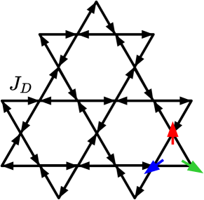
Figure 1: Definition of the bond orientations $\langle\overrightarrow{i,j}\rangle$ that determine the sign of the out-of-plane DM interactions in the Hamiltonian of Eq. (1). The orientation of the three spins in the unit cell for the ${\bf Q}=(0,0)$ magnetic order is also shown.

The spin Hamiltonian is defined by

$${\cal H}=J\sum_{\langle i,j\rangle}\mathbf{S}_{i}\cdot\mathbf{S}_{j}+J_{D}\sum_{\langle\overrightarrow{i,j}\rangle}\left(S^{x}_{i}S^{y}_{j}-S^{y}_{i}S^{x}_{j}\right),$$ (1)

where $\mathbf{S}_{i}=(S^{x}_{i},S^{y}_{i},S^{z}_{i})$ is the $S=1/2$ spin operator on site $i$ and $\langle\dots\rangle$ indicates nearest-neighboring sites. The super-exchange coupling $J$ is invariant under $i\leftrightarrow j$, while the DM term $J_{D}$ changes sign when exchanging $i$ and $j$, thus an orientation of the bonds needs to be specified in order to fully determine the Hamiltonian. The orientations, denoted by $\langle\overrightarrow{i,j}\rangle$, are represented by the arrows sketched in Fig. 1.

2.1 Tensor-network states

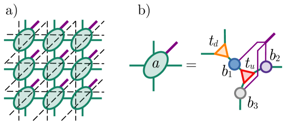
Figure 2: TN Ansätze for the kagome lattice. (a) The iPEPS state is defined by a single rank-5 on-site tensor $a$ associated to every down-pointing triangle of kagome lattice. The physical index of $a$ (violet) with dimension $d_{p}=2^{3}$ runs over all states of the three spin-$1/2$ degrees of freedom on vertices of down-pointing triangles. (b) The iPESS state is defined by the on-site tensor $a$, which is obtained by a contraction of five rank-3 tensors: Two trivalent tensors $t_{u}$ and $t_{d}$ associated to up- and down-pointing triangles, respectively, and three bond tensors $b_{1}$, $b_{2}$, and $b_{3}$, each one with single physical index (violet) representing one of the spin-$1/2$ degrees of freedom on vertices of down-pointing triangles. All auxiliary indices (green) of iPEPS and iPESS have bond dimension $D$.

TN calculations are based upon iPEPS [38] and iPESS [39, 40], which are constructed from an effective square lattice and a few tensors that contain the variational parameters. In particular, the iPEPS Ansatz approximates the ground states by a single rank-5 tensor $a$ placed at every down-pointing triangle of kagome lattice, see Fig. 2(a). The tensor $a^{s}_{uldr}$ has a physical index $s$ of dimension $d_{p}=2^{3}$, which runs over all spin states of the down-pointing triangle, and four auxiliary indices $u$, $l$, $d$, and $r$, with bond dimension $D$ corresponding to the directions of the square lattice. Then, the total number of variational parameters of this iPEPS is $d_{p}\times D^{4}$. Instead, the iPESS Ansatz restricts the form of on-site tensor $a$, defining it by a contraction of five rank-3 tensors, see Fig. 2(b). Two trivalent tensors $t_{u}$ and $t_{d}$, each with three auxiliary indices of bond dimension $D$, encode states of virtual degrees of freedom associated to up- and down-pointing triangles. Three bond tensors $b_{1}$, $b_{2}$, and $b_{3}$ host the physical spin-$1/2$ degrees of freedom and connect these trivalent tensors. Each bond tensor has two auxiliary indices of bond dimension $D$ and a physical index of dimension $2$. Therefore, the number of variational parameters in the iPESS Ansatz is $2\times D^{3}+3\times 2D^{2}$. The iPESS is constructed to treat bonds of kagome lattice faithfully, at the expense of variational freedom, whereas iPEPS favours bonds within up-pointing triangles. With growing $D$ these Ansätze are expected to reconcile. The expectation values of the Hamiltonian and local observables (e.g., $m^{2}$, the square of the magnetization) are evaluated using the corner-transfer matrix (CTM) method [52]. The CTM approximates the contraction of infinite networks by using a set of environment tensors $\{C,T\}$ with characteristic size $\chi$, dubbed environment bond dimension. The elements of these tensors are highly non-linear functions of the original tensor $a$. The variational energy is minimized by optimizing the elements of $a$ (for iPEPS) or tensors $t_{u}$, $t_{d}$, $b_{1}$, $b_{2}$, and $b_{3}$ (for iPESS), by employing the gradient descent method. The gradients are evaluated by automatic differentiation. The implementation of these Ansätze with CTM method and their optimization is provided by the peps-torch library [53]. In general, for fixed bond dimension $D$, iPEPS has lower variational energy and smaller magnetization than iPESS (since the iPEPS state has more variational parameters than the iPESS one). Quantitative comparisons between iPEPS and iPESS are reported in the Appendix A.

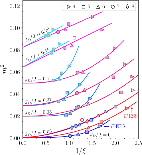
Figure 3: Finite-correlation length scaling of the antiferromagnetic order parameter (squared) $m^{2}$, for both iPEPS and iPESS Ansätze with bond dimension $D$ ranging from $4$ to $8$. The power-law fittings of Eqs. (2), (3), (4), and (5) are employed. The empty markers are excluded in the fits shown here, but contribute to the determination of the error bar on the extrapolated results.

All the tensor-network calculations are performed with finite values of the CTM environment dimension $\chi$ and the bond dimension $D$. The thermodynamic limit is then reached by taking $\chi\to\infty$ for each $D$ and then $D\to\infty$. To achieve the limit of $D\to\infty$, we use the finite-correlation length scaling [42, 43], which gives more accurate results than the straightforward $1/D$ extrapolation. Here, the correlation length $\xi$ of an infinite-size TN state plays the role of infrared cut-off, analogously to the linear lattice size of numerical methods based on finite-size calculations. An important aspect of our scaling analysis is that the same thermodynamic value of $m^{2}$ is imposed for both iPEPS and iPESS data, since they are expected to converge to the same (exact) ground state. For the magnetic phase with relatively large magnetization (i.e., for large values of $J_{D}/J>0.1$), we consider the fitting functions:

$$m_{\text{iPEPS}}^{2}(\xi)=m^{2}(\infty)+a/\xi,$$ (2)

$$m_{\text{iPESS}}^{2}(\xi)=m^{2}(\infty)+b/\xi.$$ (3)

By contrast, within the spin-liquid and weakly-ordered regimes (i.e., for small values of $J_{D}/J\leq 0.1$), an empirical fit turns out to be more suitable:

$$m_{\text{iPEPS}}^{2}(\xi)=m^{2}(\infty)+a/\xi^{b},$$ (4)

$$m_{\text{iPESS}}^{2}(\xi)=m^{2}(\infty)+c/\xi^{d}.$$ (5)

The smoothness of the scaling in both spin-liquid and magnetically ordered phases is demonstrated in Fig. 3 for a few values of $J_{D}/J$. The value of the thermodynamic magnetization is obtained by performing different extrapolations using different sets of points. The final $m^{2}$ value corresponds to the best fit (i.e., the fit with smallest fitting error) and the error bar is determined by combining the results of the different extrapolations. We emphasize that the variational optimization provides data with higher quality then the simple-update method used in Ref. [26] and is crucial for extrapolations, see Appendix A for a detailed discussion.

2.2 Gutzwiller-projected wave functions

VMC calculations are performed by using Gutzwiller-projected wave functions [54, 55, 56], constructed from the Abrikosov-fermion representation of the spin operators [57, 58, 59], $\mathbf{S}_{i}=\frac{1}{2}\sum_{\alpha,\beta}$ $c_{i,\alpha}^{\dagger}\bm{\sigma}_{\alpha,\beta}c_{i,\beta}^{\phantom{\dagger}}$, and the definition of an auxiliary Hamiltonian containing hoppings and a Zeeman field:

$${\mathcal{H}}_{\rm 0}=\sum_{\langle i,j\rangle,\alpha}\chi_{ij}^{\alpha}c_{i,\alpha}^{\dagger}c_{j,\alpha}+h\sum_{i}\mathbf{M}_{i}\cdot\mathbf{S}_{i}.$$ (6)

The first term is a nearest-neighbor hopping, including both “singlet” ($\chi_{ij}^{\uparrow}=\chi_{ij}^{\downarrow}$) and “triplet” ($\chi_{ij}^{\uparrow}=-\chi_{ij}^{\downarrow}$) complex-valued amplitudes [33]. In particular, we find that the optimal variational Ansatz contains a real singlet hopping and a purely imaginary triplet hopping [33], which reduces to the $U(1)$ Dirac state [60, 61] when restricted to the singlet part. The second term (for $h\neq 0$) induces magnetic order in the $XY$ plane, with the periodicity determined by the unit vector ${\mathbf{M}_{i}=[\cos({\bf Q}\cdot{\bf R}_{i}+\phi_{i}),\sin({\bf Q}\cdot{\bf R}_{i}+\phi_{i}),0]}$ (where ${\bf Q}$ is the pitch vector, ${\bf R}_{i}$ is the coordinate of the unit cell of site $i$, and $\phi_{i}$ is a sublattice-dependent angle). In the following, we consider the ${\bf Q}=(0,0)$ case, with $\phi_{i}$ giving $120^{\circ}$ order in all triangles (as sketched in the inset of Fig. 1), which is suitable for the out-of-plane DM interaction. The full variational wave function $|\Psi_{0}\rangle$ is built from the ground state $|\Phi_{0}\rangle$ of the Hamiltonian (6), applying the Gutzwiller projector, which enforces single fermionic occupations, ${{\cal P}_{G}=\prod_{i}(n_{i,\uparrow}-n_{i,\downarrow})^{2}}$, where ${n_{i,\alpha}=c_{i,\alpha}^{\dagger}c_{i,\alpha}^{\phantom{\dagger}}}$. In addition, a projector onto the subspace with $S^{z}=\sum_{i}S^{z}_{i}=0$ and a spin-spin Jastrow factor ${{\cal J}=\exp\left(1/2\sum_{i,j}v_{i,j}S^{z}_{i}S^{z}_{j}\right)}$ (where $v_{i,j}$ are variational parameters) are included:

$$|\Psi_{0}\rangle={\cal J}{\cal P}_{S_{z}=0}{\cal P}_{G}|\Phi_{0}\rangle.$$ (7)

Calculations are done on $N=3\times L\times L$ clusters and extrapolations to the thermodynamic limit are performed using standard finite-size scaling analysis [62, 63]. In Fig. 4, we show the extrapolation of the order parameter $m^{2}$ as a function of $L$, for several values of the ratio $J_{D}/J$. For $J_{D}/J<0.03$, the magnetization curves are fitted with a $1/L^{2}$ behavior.

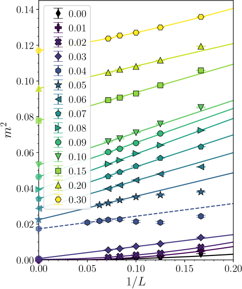
Figure 4: Finite-size scaling of the antiferromagnetic order parameter (squared) $m^{2}$ as computed by VMC. Different colors/markers indicate different values of $J_{D}/J$, as reported in the box.

Within the present variational approach, we can also define a set of excitations to approximate the low-energy spectrum of the system and compute the dynamical spin-spin correlations [44]. In fact, approximate excited states are constructed by linear superpositions of particle-hole (spinon) excitations, whose coefficients are determined by the Rayleigh-Ritz variational principle. Although the recipe to define two-spinon excitations with $S^{z}=0$ has been discussed in details in recent works [46, 47, 50] on frustrated spin models (with SU(2) spin symmetry), here we briefly outline the general construction for the case of a Bravais lattice with a basis, which is suitable for the kagome lattice under investigation (technical details can be found in Ref. [48]). For this purpose, we adopt an explicit notation in which sites are denoted by a Bravais vector ${\bf R}$ and a sublattice index $a$, such that $c_{i,\beta}^{\phantom{\dagger}}\to c_{R,a,\beta}^{\phantom{\dagger}}$. A (non-orthogonal) set of particle-hole spinon excitations with momentum ${\bf q}$ is defined by the states

$$|q;R,a;b\rangle=\mathcal{J}\mathcal{P}_{G}\mathcal{P}_{S^{z}=0}\sum_{R^{\prime}}e^{i{\bf q}\cdot{\bf R}^{\prime}}\left(c^{\dagger}_{R+R^{\prime},a,\uparrow}c^{\phantom{\dagger}}_{R^{\prime},b,\uparrow}-c^{\dagger}_{R+R^{\prime},a,\downarrow}c^{\phantom{\dagger}}_{R^{\prime},b,\downarrow}\right)|\Phi_{0}\rangle.$$ (8)

Then, the approximate excited states for the spin model are taken as linear combinations of $\{|q;R,a;b\rangle\}$ states

$$|\Psi_{n}^{q}\rangle=\sum_{R}\sum_{a,b}A^{n,q}_{R,a;b}|q;R,a;b\rangle,$$ (9)

where $n$ is an integer index labelling the variational excitations with momentum ${\bf q}$. The coefficients of the expansion, $A^{n,q}_{R,a;b}$, are obtained by solving the generalized eigenvalue problem

$$\sum_{R^{\prime},a^{\prime},b^{\prime}} H^{q}_{R,a;b|R^{\prime},a^{\prime};b^{\prime}}A^{n,q}_{R^{\prime},a^{\prime};b^{\prime}}$$

$$=E_{n}^{q}\sum_{R^{\prime},a^{\prime},b^{\prime}}O^{q}_{R,a;b|R^{\prime},a^{\prime};b^{\prime}}A^{n,q}_{R^{\prime},a^{\prime};b^{\prime}},$$ (10)

where $E_{n}^{q}$ are the energies of the excitations $|\Psi_{n}^{q}\rangle$, and

$$H^{q}_{R,a;b|R^{\prime},a^{\prime};b^{\prime}} = \langle q;R,a;b|\mathcal{H}|q;R^{\prime},a^{\prime};b^{\prime}\rangle$$ (11)

$$O^{q}_{R,a;b|R^{\prime},a^{\prime};b^{\prime}} = \langle q;R,a;b|q;R^{\prime},a^{\prime};b^{\prime}\rangle$$ (12)

are the Hamiltonian and overlap matrices, which can be efficiently evaluated by a suitable Monte Carlo scheme [47, 48]. Finally, assuming that all states are properly normalized, the out-of-plane dynamical structure factor is given by:

$$S^{z}({\bf q},\omega)=\sum_{n}|\langle\Psi_{n}^{q}|S^{z}_{q}|\Psi_{0}\rangle|^{2}\delta(\omega-E_{n}^{q}+E_{0}),$$ (13)

where $S^{z}_{q}=\frac{1}{\sqrt{N}}\sum_{j}e^{i{\bf q}\cdot{\bf r}_{j}}S^{z}_{j}$ (${\bf r}_{j}$ being the coordinate of site $j$); $E_{0}$ is the variational ground-state energy of $|\Psi_{0}\rangle$ defined in Eq. (7), $E_{n}^{q}$ are the energies of the excited states $|\Psi_{n}^{q}\rangle$ for the momentum ${\bf q}$, as obtained from Eqs. (9) and (2.2).

Following a similar construction, we can also define spinon excitations with $S^{z}=1$, and a different set of excited states and energies, which we still denote as $|\Psi_{n}^{q}\rangle$ and $E_{n}^{q}$, respectively, for simplicity of notation. By means of this variational set of excited states one can compute the in-plane dynamical structure factor:

$$S^{\pm}({\bf q},\omega)=\sum_{n}|\langle\Psi_{n}^{q}|S^{+}_{q}|\Psi_{0}\rangle|^{2}\delta(\omega-E_{n}^{q}+E_{0}).$$ (14)

The technical details for calculation of $S^{\pm}({\bf q},\omega)$ are reported in Appendix C.

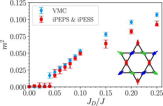
Figure 5: Antiferromagnetic order parameter (squared) at ${\bf Q}=(0,0)$ as a function of $J_{D}/J$. Both VMC and TN results are reported, as extrapolated in the thermodynamic limit (which is obtained by standard finite-size extrapolation ${L\to\infty}$ for VMC and finite-correlation-length scaling ${\xi\to\infty}$ for TN, combining iPEPS and iPESS results). The inset shows the ${\bf Q}=(0,0)$ coplanar order induced by the presence of the out-of-plane DM interaction.

3 Results

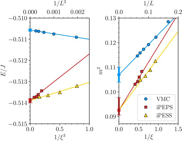
Figure 6: Thermodynamic extrapolations for VMC and TN (both iPEPS and iPESS) data for the ground-state energy per site (left panel) and the antiferromagnetic order parameter (squared) at ${\bf Q}=(0,0)$ (right panel), for $J_{D}/J=0.25$. VMC results are obtained on $3\times L\times L$ clusters and extrapolations are performed by using standard finite-size analysis for ${L\to\infty}$ (as shown in the upper $x$-axis). TN results are obtained by fixing the bond dimension $D$, evaluating the correlation length $\xi$, and then performing the finite-correlation-length scaling for $\xi\to\infty$ (as shown in lower $x$-axis).

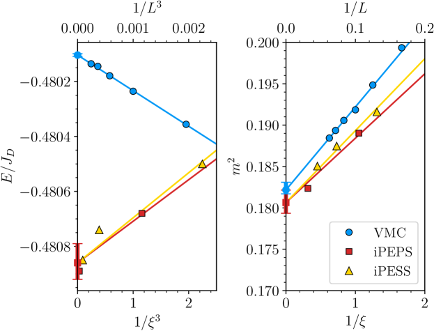
Figure 7: The same as in Fig. 6 for $J=0$ and $J_{D}=1$, i.e., the model with only DM interaction.

In this section, we discuss the numerical results that have been obtained within TN and VMC approaches. First, we show the ground-state properties, focusing on the magnetization curve when $J_{D}/J$ is varied from $0$ to $0.25$ (suitable for YCu₃(OH)₆Cl₃), including ${J_{D}/J=0.18}$ (suitable for Cs₂Cu₃SnF₁₂). Then, we present the results for the dynamical spin correlations, as obtained within the VMC technique. In particular, we concentrate on the case with $J_{D}/J=0.18$, which allows us to highlight the remarkable similarities between the experimental outcome of Ref. [23] and the spectral functions of the Hamiltonian (1).

3.1 Static properties: energy and magnetization

The results of the squared magnetization $m^{2}$ at ${\bf Q}=(0,0)$ for increasing values of $J_{D}/J$ are reported in Fig. 5, comparing VMC and TN results. Within VMC, we compute $m^{2}$ by evaluating the spin-spin correlations at the maximum distance for various cluster sizes $L$ and then perform the extrapolation $L\to\infty$. Within iPEPS and iPESS, instead, we measure the local magnetization $m^{2}=|\langle\vec{S}\rangle|^{2}$ (which is identical on every site with high precision) for different values of the bond dimension $D$. Then we perform the finite-correlation-length scaling, imposing the same extrapolated value for iPEPS and iPESS, which helps reducing the error in the thermodynamic estimate. Technical details have been discussed in Section 2. The transition between the magnetically disordered regime and the magnetically ordered phase is found to be in excellent agreement between VMC and TN techniques. Indeed, the transition point is estimated at $J_{D}/J=0.030(5)$ by VMC and $0.040(5)$ by iPEPS and iPESS. We mention that separate fits of iPESS and iPEPS datasets locate the transition at $J_{D}/J=0.04\textrm{-}0.05$, in agreement with the estimate obtained by combining the data in a single extrapolation. Similarly to the results of Ref. [26], our estimate for the $J_{D}/J$ value at the transition is considerably smaller than the one reported in Ref. [24] ($J_{D}/J\approx 0.1$). The latter is obtained by exact diagonalization on small clusters (up to $36$ sites) and the extrapolation of the order parameter to the thermodynamic limit is affected by strong finite size effects, especially close to the phase transition. According to the VMC wave function, the magnetically disordered phase found for $0<J_{D}/J\lesssim 0.03$ is a spin liquid state with a finite gap in the spinon spectrum (see Appendix B). The spinon gap closes in the Heisenberg limit ($J_{D}=0$) where the variational state reduces to the $U(1)$ Dirac spin liquid [60, 61].

Close to the transition point, the magnetizations obtained with VMC and TN are compatible within the errorbar, except for $J_{D}/J=0.04$, for which the TN estimation of $m^{2}$ is very small, while a finite value is obtained within VMC. For larger values of the DM interaction, i.e., $J_{D}/J\gtrsim 0.15$, VMC and TN give comparable values of $m^{2}$, the maximum difference being about $20\%$. Finally, for very large values of $J_{D}/J$, the agreement between VMC and TN is again excellent. For example, for the pure DM model with $J=0$ (and $J_{D}=1$), the energy difference between the two methods is smaller than $10^{-3}J_{D}$ and the estimated values of the order parameter, $m^{2}\approx 0.181$ (TN) and $m^{2}\approx 0.182$ (VMC), are compatible within errobars. These values of $m^{2}$ are also in good agreement with the one reported in Ref. [24], once the latter is corrected by a factor $1/2$ due to a different definition of the order parameter. The actual comparison between TN and VMC is highlighted in Figs. 6 and 7, where we report both energy and magnetization (squared) for $J_{D}/J=0.25$ and $J=0$, respectively. We remark that, in all cases we examined, the largest difference between the extrapolated energies $\Delta E=E_{\rm VMC}-E_{\rm TN}$ is small and it is found in the Heisenberg model limit (i.e., $J_{D}=0$), where $\Delta E/J\approx 0.007$.

3.2 Dynamical properties: spin correlation functions

Let us now focus on the low-energy spectrum as detected by the dynamical spin structure factor. Since, in presence of a finite DM interaction the SU(2) spin symmetry is explicitly broken, we consider both in-plane $S^{\pm}({\bf q},\omega)$ and out-of-plane $S^{z}({\bf q},\omega)$ responses. Before discussing the VMC results, it is instructive to look at the outcome of the linear spin-wave (LSW) approach, i.e., the simplest approximation for the low-energy spectrum of the ordered phase [64] (white lines in Fig. 8, for $J_{D}/J=0.18$). Here, the spectral weight is concentrated on three magnon modes. One of them, representing the Goldstone mode, is gapless at $\Gamma$ (i.e., the center of the Brillouin zone) and $\Gamma^{\prime}$ (i.e., the midpoint of the edges of the extended Brillouin zone). Its maximal intensity is observed in the in-plane response at $\Gamma^{\prime}$, see Fig. 8 for $J_{D}/J=0.18$. The other two magnon branches are gapped, one having a completely flat dispersion, and show the largest weight around the $\Gamma^{\prime}$ point in the out-of-plane correlations. We mention that the LSW approximation can be reproduced within our VMC approach by taking no spinon hopping in the auxiliary Hamiltonian that defines the unprojected wave funtion (see Section 2), such that its ground state becomes a spin produt state in real space [65] (for that, the presence of the spin-spin Jastrow factor is fundamental to reproduce the correct magnon dispersions). In order to go beyond the LSW approach and assess both the renormalization of magnon branches and the presence of a continuum at low energies, we employ the dynamical VMC previously discussed.

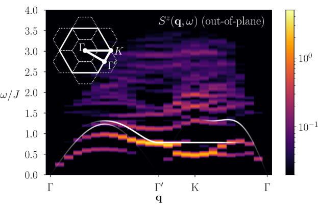
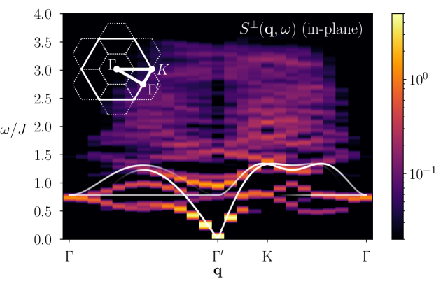
Figure 8: Out-of-plane [$S^{z}({\bf q},\omega)$, upper panel] and in-plane [$S^{\pm}({\bf q},\omega)$, lower panel] spin dynamical structure factor, as computed by dynamical VMC, see Eqs. (13) and (14), for $J_{D}/J=0.18$. Calculations are performed on the $3\times 12\times 12$ cluster. LSW results for the three magnon modes are also shown for comparison (the intensity of the signal is proportional to the thickness of the white lines; notice that a different scale for the in-plane and out-of-plane components is used) [64]. The inset in the upper left corner of the figures shows the first and extended Brillouin zones of the kagome lattice (with dashed and solid lines, respectively), and the high symmetry points $\Gamma$ and $\Gamma^{\prime}$.

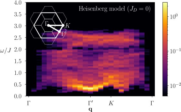
Figure 9: $S^{z}({\bf q},\omega)$ spin dynamical structure factor, as computed by the VMC approach, see Eqs. (13), for the Heisenberg model with $J_{D}=0$. Calculations are performed on the $3\times 12\times 12$ cluster.

The variational results for both in-plane and out-of-plane dynamical correlations are shown in Fig. 8, for $J_{D}/J=0.18$, along the high-symmetry path $\Gamma-\Gamma^{\prime}-K-\Gamma$ (qualitatively similar results are obtained for ${J_{D}/J=0.25}$). Additional spectral functions, close to the the quantum phase transition, are reported in Appendix C. Within the low-energy portion of the VMC spectrum, the three magnon branches can be recognized thanks to their different intensities in the $S^{z}({\bf q},\omega)$ and $S^{\pm}({\bf q},\omega)$ channels, which can be matched to the LSW predictions. The first aspect that is worth noticing when comparing the outcome of the variational calculations with the LSW theory is the sensible downward renormalization of the magnon dispersion, which has been also discussed in the analysis of experimental measurements [66]. Indeed, both the gapless and the gapped dispersive branches are squeezed in energy, with a corresponding reduced velocity of the Goldstone mode around $\Gamma^{\prime}$; by contrast, the flat magnon branch of the LSW theory acquires a (small) dispersion in the VMC spectrum, as can be seen in the in-plane response. Most importantly, the variational approach is able to describe a broad continuum above the magnon branches, i.e., a dense bunch of excitations with moderate weights which extends up to $\omega/J\approx 3.5$. Within the continuum, a relatively intense and weakly dispersing (damped) mode exists around $\Gamma^{\prime}$, right above the three magnon excitations, clearly visible in the in-plane structure factor. This is a genuine hallmark of the dynamical structure factor when magnetic order develops beyond the quantum critical point; indeed, in the Heisenberg model with no DM interaction, the spectrum looks very broad and uniform, with no particular features in the continuum, see Fig. 9. The energy of the damped mode is $\omega\approx J$, very similar to the one observed within the inelastic neutron scattering in Cs₂Cu₃SnF₁₂ [23]. The outcome clearly suggests that the continuum is not featureless, but instead possesses non-trivial aspects that go beyond what can be captured by the simple LSW approximation.

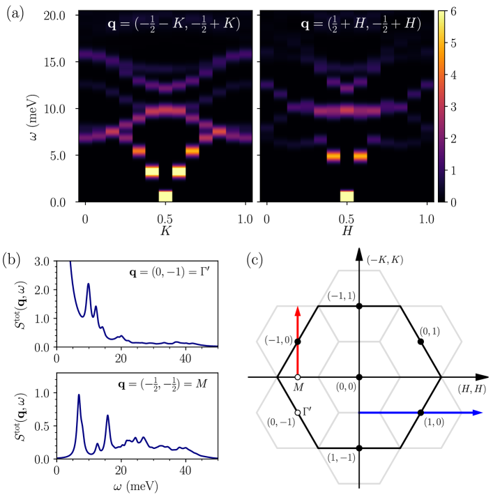
Figure 10: Panel (a): Total spin dynamical structure factor $S^{\rm tot}({\bf q},\omega)=S^{z}({\bf q},\omega)+S^{\pm}({\bf q},\omega)$ for $J_{D}/J=0.18$ on the $3\times 12\times 12$ cluster, along the cuts in momentum space shown in panel (c), reproducing the ones used in Ref. [23]. Here, the super-exchange coupling has been fixed to $J=12.8$ meV and $J_{D}/J=0.18$, as estimated in Ref. [23] for Cs₂Cu₃SnF₁₂. Panel (b): The dynamical structure factor as a function of $\omega$ at $\Gamma^{\prime}$ and $M$ points (a broadening of $\sigma=0.05J$ has been introduced to have a smooth curve). Panel (c): first (grey hexagons) and extended (black hexagon) Brillouin zones of the kagome lattice. The red and blue arrows depict the paths along $\mathbf{q}=(-\frac{1}{2}-K,-\frac{1}{2}+K)$ and $\mathbf{q}=(\frac{1}{2}+H,-\frac{1}{2}+H)$ considered in panel (a). The empty dots indicate the $\Gamma^{\prime}$ and $M$ points considered in panel (b).

The similarity between our VMC results and the experimental outcome is also evident from Fig. 10, where we report the total dynamical structure factor $S^{\rm tot}({\bf q},\omega)=S^{z}({\bf q},\omega)+S^{\pm}({\bf q},\omega)$ along the cuts in momentum space considered in Ref. [23]. For a direct comparison, we take $J=12.8$ meV, as estimated within the experimental work. Even though only a few ${\bf q}$ points are available along these cuts in the $3\times 12\times 12$ cluster, the global picture emerges. The most intense signal appears at very low energy around the $\Gamma^{\prime}$ point [obtained for $K=1/2$ and $H=1/2$ in the $x$ axes of Fig. 10(a)], corresponding to the gapless Goldstone mode; the other two (gapped) magnons are mostly visible around $\Gamma^{\prime}$, where their energies almost coincide, i.e., $\omega\approx 10$ meV. On top of these magnon modes, an additional branch is also visible, with the maximum intensity at $\omega\approx 13$ meV (again at $\Gamma^{\prime}$) and an upturning dispersion. This latter feature can be directly related to the one reported between $12$ and $14$ meV in inelastic neutron scattering experiments [23]. However, the relative intensities of the experimental peaks are not fully reproduced; in particular, at the $M$ point, the high-energy peak at $\omega\approx 15$ meV has a relatively large intensity, which is almost equal to the one of the magnons at $\omega\approx 7$ meV, see Fig. 10(b). By contrast, in experiments this feature is not observed. In general, a close comparison between the experimental results and numerical calculations is very difficult and goes beyond the scope of the present work. Indeed, many details (e.g., further super-exchange couplings, anisotropies, and disorder effects) may affect the outcome. In addition, within our variational approach, the number of excited states is limited by the cluster size; as a consequence, providing a reliable estimate for the boundaries of the continuum is not possible. Nevertheless, our results strongly suggest that the broad peak observed at $\Gamma^{\prime}$ is located above the magnon modes and can be thus expected to lie inside the continuum of excitations. The presence of an intense signal above the three magnon modes is a genuine feature of the model that cannot be described within a single-magnon picture.

4 Discussion

By employing a combination of VMC and TN methods, we have shown that the spin-$1/2$ kagome antiferromagnet develops a finite ${\bf Q}=(0,0)$ magnetic order when an out-of-plane DM interaction $J_{D}$ exceeds a small fraction $0.03\mathrm{-}0.04$ of the nearest-neighbor super-exchange $J$. In view of these results, a simple model with only $J$ and $J_{D}$ may not be suitable for the description of the Herbertsmithite material, since the value of $J_{D}$ interaction has been estimated to be above the critical value found here, while the compound does not show any sign of magnetic ordering down to the lowest temperature. In this regard, additional ingredients (e.g., substitutional disorder) should be included for a proper description of this material. By contrast, we believe that a model with only $J$ and DM interaction $J_{D}$ (above the critical value) may well capture the main features (at least at low temperature) of both Cs₂Cu₃SnF₁₂ and YCu₃(OH)₆Cl₃ materials. In particular, the dynamical structure factor of this minimal model can be directly compared to the results of inelastic neutron-scattering experiments on Cs₂Cu₃SnF₁₂. Within the magnetically ordered phase, besides the magnon branches, the existence of additional damped mode in the continuum is reported, in close similarity to what has been recently detected in Cs₂Cu₃SnF₁₂ [23]. Open questions remain to fully characterize the magnetically disordered regime. Within the Gutzwiller-projected fermionic approach, a triplet hopping develops as soon as $J_{D}$ is finite, opening a gap in the spinon spectrum. Nevertheless, the incipient magnetic phase does not allow the stabilization of a spin liquid state with a sufficiently large gap to be detected within the available numerical calculations, whose momentum resolution is limited by finite size effects. Understanding whether a detectable gapped state may exist when suitable perturbations are added on top of the Heisenberg model is an important issue that should be further addressed in future investigations.

Appendix A Details on the tensor network calculations

A.1 Extrapolations as a function of the CTM environment bond dimension $\chi$

For each fixed bond dimension $D$, the variational optimization are performed with different CTM environment bond dimensions $\chi$. Then, observables are evaluated for each value $\chi$ and finally etrapolated for $\chi\to\infty$. We show the case with $J_{D}/J=0.02$ in Fig. 11. In practice, local observables (e.g., energy and magnetization) converge very rapidly, with small linear corrections in $1/\chi$; instead, the correlation length displays slightly larger corrections, which typically require a quadratic fitting.

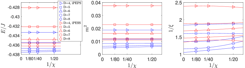
Figure 11: Extrapolations of the energy, magnetization (square), and correlation length as a function of the CTM environment dimension $\chi$ for $J_{D}/J=0.02$.

A.2 Analysis of Ansätze and optimizations

Here, we analyze the TN data in terms of Ansätze and optimizations. First, we consider the variational optimization, as adopted in this work, and compare energies and magnetizations for iPESS and iPEPS Ansätze, see Fig. 12. For every fixed value of $D$, iPEPS has lower energy and smaller magnetization than iPESS. This is due to the fact that the latter one is more constrained. On the other hand, symmetry properties of iPESS are better preserved, since iPESS treats down-pointing and up-pointing triangles equally, while in iPEPS only the entanglement inside the down-pointing triangle is restricted by finite $D$ (similar to the 9-iPESS Ansatz defined in Ref. [40]). In the worst case (i.e., within the spin liquid regime), the difference of the energy contributions coming from different bonds is about $1\%$ for the iPEPS with $D=7$ (the point-group symmetries are expected to be restored only for $D\to\infty$).

We now briefly discuss the comparison between variational and simple update (SU) method to optimize the TN states. Within the former approach, the tensors of iPESS and iPEPS states are optimized by using gradients of the total energy, taking into account the global environment. By contrast, the SU approach ignores the non-local environment tensors during optimization and is only applicable to the iPESS Ansatz [26]. The comparison of these methods for energies and magnetizations is shown in Fig. 12. For each bond dimension $D$, the two optimization techniques give similar energies (the variational one being slightly lower), but within the SU approach the magnetization is overestimated by roughly $10\%$ and the correlation length is considerably underestimated. The good quality provided by the variational optimization is particularly important when performing scalings. Indeed, while the extrapolations of $m^{2}$ are quite smooth within the variational approach, the behavior obtained within the SU technique is more erratic and may lead to unphysical negative values for the extrapolated quantities.

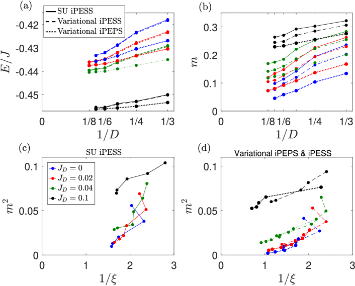
Figure 12: Comparison between SU iPESS (solid line), variational iPESS (dashed line) and variational iPEPS (dotted line) for different values of $J_{D}/J$ and $\chi=80$. Panels (a) and (b): energies and magnetizations as a function of $1/D$. Panels (c) and (d): square of magnetizations as a function of $1/\xi$ for SU and variational optimizations.

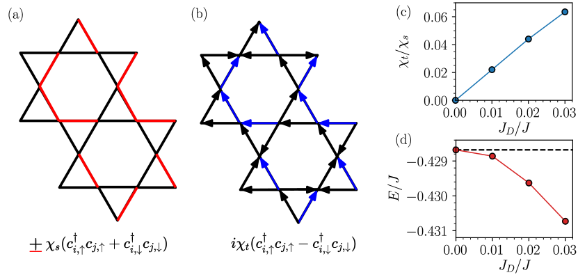
Figure 13: Spin liquid wave function used within the VMC approach. Panel (a): sign pattern of the real-valued singlet hoppings of the auxiliary Hamiltonian $\mathcal{H}_{0}$, with black (red) bonds denoting $\chi_{s}$ ($-\chi_{s}$) terms. This variational Ansatz corresponds to the Dirac spin liquid state [60, 61, 27]. Panel (b): sign pattern of the imaginary triplet hoppings of the auxiliary Hamiltonian $\mathcal{H}_{0}$. The arrows from $i\rightarrow j$ represent the triplet term $i\chi_{t}(c^{\dagger}_{i,\uparrow}c_{j,\uparrow}-c^{\dagger}_{i,\downarrow}c_{j,\downarrow})$, which is odd under the exchange of $i$ and $j$ sites. Note that the orientations of the black (blue) arrows is equal (opposite) to the ones of the DM interaction (see Fig. 1). Panel (c): optimal values of the ratio $\chi_{t}/\chi_{s}$ for the spin-liquid Ansatz in the thermodynamic limit. Panel (d): thermodynamic limit of the variational energy of the spin liquid state (with no Zeeman field and no Jastrow factor). The dashed line indicates the energy of the Dirac spin liquid state, which is independent on the value of $J_{D}$.

Appendix B Spin liquid wave function of VMC

The Gutzwiller-projected wave functions employed in the VMC approach are defined by means of the auxiliary Hamiltonian (6), which contains hopping terms and a Zeeman field that induces ${\bf Q}=(0,0)$ magnetic order in the $XY$ plane. For $J_{D}/J\lesssim 0.03$, the Zeeman field parameter $h$ is found to vanish in the thermodynamic limit, signalling the onset of a spin-liquid phase, which is described by the Hamiltonian with only hopping terms. The optimal variational Ansatz contains a real singlet hopping ($\chi_{s}$) and an imaginary triplet hopping ($\chi_{t}$) at first-neighbors. The sign structure of the hoppings is dictated by the projective symmetry group [33] and is schematically represented in Fig. 13. In the Heisenberg limit, $J_{D}=0$, $\chi_{t}$ vanishes (exactly) upon minimization of the variational energy and the auxiliary Hamiltonian reduces to the one of the $U(1)$ Dirac spin-liquid state [60, 61, 27], with gapless Dirac points in the spinon spectrum. On the other hand, for any $J_{D}/J>0$, the variational optimization of the wave function yields a finite value of the triplet hopping $\chi_{t}$ (see Fig. 13), which opens a gap in the spinon spectrum and provides a variational energy gain with respect to the Dirac spin-liquid state (whose energy is independent on the value of $J_{D}$). Unfortunately, we cannot give definitive statemets on the nature of the spin-liquid regime (e.g., whether it is a $U(1)$ or $\mathbb{Z}_{2}$ state), because additional superconducting pairings can be stabilized in the auxiliary Hamiltonian upon numerical optimizations [33], although they do not provide an appreciable energy gain.

Appendix C Dynamical variational Monte Carlo

As discussed in the main text, we compute both in-plane [$S^{\pm}({\bf q},\omega)$] and out-of-plane [$S^{z}({\bf q},\omega)$] dynamical structure factor by VMC. A detailed discussion of the method to compute $S^{z}({\bf q},\omega)$ is given in Refs. [46, 47, 48]. Here, we present an extension of the dynamical VMC technique for the calculation of the $S^{\pm}({\bf q},\omega)$ component.

Starting from the optimal fermionic wave function $|\Phi_{0}\rangle$, we define a set of projected particle-hole excitations with momentum ${\bf q}$ as follows

$$|q;R,a;b\rangle=\mathcal{J}\mathcal{P}_{G}\mathcal{P}_{S^{z}=1}\sum_{R^{\prime}}e^{i{\bf q}\cdot{\bf R}^{\prime}}c^{\dagger}_{R+R^{\prime},a,\uparrow}c^{\phantom{\dagger}}_{R^{\prime},b,\downarrow}|\Phi_{0}\rangle.$$ (15)

Here and in the following, we label lattice sites by specifying their Bravais lattice vector ${\bf R}$ (or ${\bf R^{\prime}}$) and their sublattice index, denoted by Latin letters, e.g., $a$ (or $b$). Then, we construct variational excited states for the system by taking linear combinations of the particle-hole excitations $|q;R,a;b\rangle$, namely

$$|\Psi_{n}^{q}\rangle=\sum_{R}\sum_{a,b}B^{n,q}_{R,a;b}|q;R,a;b\rangle,$$ (16)

where $n$ is an integer label. The coefficients $B^{n,q}_{R,a;b}$ are obtained by the Rayleigh-Ritz method, i.e., by solving the generalized eigenvalue problem

$$\sum_{R^{\prime},a^{\prime},b^{\prime}} H^{q}_{R,a;b|R^{\prime},a^{\prime};b^{\prime}}B^{n,q}_{R^{\prime},a^{\prime};b^{\prime}}$$

$$=E_{n}^{q}\sum_{R^{\prime},a^{\prime},b^{\prime}}O^{q}_{R,a;b|R^{\prime},a^{\prime};b^{\prime}}B^{n,q}_{R^{\prime},a^{\prime};b^{\prime}}.$$ (17)

for each desired momentum ${\bf q}$. Here, $E_{n}^{q}$ are the energies of the excitation $|\Psi_{n}^{q}\rangle$, and

$$H^{q}_{R,a;b|R^{\prime},a^{\prime};b^{\prime}} = \langle q;R,a;b|\mathcal{H}|q;R^{\prime},a^{\prime};b^{\prime}\rangle$$ (18)

$$O^{q}_{R,a;b|R^{\prime},a^{\prime};b^{\prime}} = \langle q;R,a;b|q;R^{\prime},a^{\prime};b^{\prime}\rangle$$ (19)

are the Hamiltonian and overlap matrices, respectively. Their entries are computed stochastically by a suitable Monte Carlo scheme, which is outlined in the following for the case of the overlap matrix (the Hamiltonian matrix can be treated analogously). By inserting a resolution of the identity over fermionic configurations $\{|x\rangle\}$, we can write

$$O^{q}_{R,a;b|R^{\prime},a^{\prime};b^{\prime}}=\sum_{x}\langle q;R,a;b|x\rangle\langle x|q;R^{\prime},a^{\prime};b^{\prime}\rangle.$$ (20)

Due to the presence of $\mathcal{P}_{G}$ and $\mathcal{P}_{S^{z}=1}$ in the definition of $|q;R,a;b\rangle$ states [see Eq. (15)], the states $\{|x\rangle\}$ are constrained to one-fermion-per-site configurations with $S^{z}=1$. Therefore, we can compute the entries of the overlap matrix by a Metropolis algorithm in which we sample the Hilbert space according to the probability function $|\langle x|\Psi_{0}^{\prime}\rangle|^{2}/\|\Psi_{0}^{\prime}\|^{2}$, where $|\Psi_{0}^{\prime}\rangle={\cal J}{\cal P}_{S_{z}=1}{\cal P}_{G}|\Phi_{0}\rangle$ and $\|\Psi_{0}^{\prime}\|^{2}=\langle\Psi_{0}^{\prime}|\Psi_{0}^{\prime}\rangle$. Thus, we can evaluate the rescaled overlap matrix

$$\tilde{O}^{q}_{R,a;b|R^{\prime},a^{\prime};b^{\prime}} =\frac{O^{q}_{R,a;b|R^{\prime},a^{\prime};b^{\prime}}}{\|\Psi_{0}^{\prime}\|^{2}}=\sum_{x}\frac{|\langle x|\Psi_{0}^{\prime}\rangle|^{2}}{\|\Psi_{0}^{\prime}\|^{2}}$$

$$\times\left[\frac{\langle q;R,a;b|x\rangle}{\langle\Psi_{0}^{\prime}|x\rangle}\frac{\langle x|q;R^{\prime},a^{\prime};b^{\prime}\rangle}{\langle x|\Psi_{0}^{\prime}\rangle}\right].$$ (21)

An analogous formula applies for the calculation of a rescaled Hamiltonian matrix

$$\tilde{H}^{q}_{R,a;b|R^{\prime},a^{\prime};b^{\prime}} =\frac{H^{q}_{R,a;b|R^{\prime},a^{\prime};b^{\prime}}}{\|\Psi_{0}^{\prime}\|^{2}}=\sum_{x}\frac{|\langle x|\Psi_{0}^{\prime}\rangle|^{2}}{\|\Psi_{0}^{\prime}\|^{2}}$$

$$\times\left[\frac{\langle q;R,a;b|x\rangle}{\langle\Psi_{0}^{\prime}|x\rangle}\frac{\langle x|\mathcal{H}|q;R^{\prime},a^{\prime};b^{\prime}\rangle}{\langle x|\Psi_{0}^{\prime}\rangle}\right].$$ (22)

Then, we solve the generalized eigenvalue problem of Eq. (C) with the rescaled matrices. The resulting $B^{n,q}_{R,a;b}$ coefficients are normalized such that

$$\sum_{R,R^{\prime}}\sum_{a,a^{\prime}}\sum_{b,b^{\prime}}[B^{n,q}_{R,a;b}]^{*}\tilde{O}^{q}_{R,a;b|R^{\prime},a^{\prime};b^{\prime}}B^{m,q}_{R^{\prime},a^{\prime};b^{\prime}}=\delta_{n,m}.$$ (23)

As a consequence, the variational excited states satisfy $\langle\Psi_{n}^{q}|\Psi_{m}^{q}\rangle=\|\Psi_{0}^{\prime}\|^{2}\delta_{n,m}$.

The excited state energies $\{E_{n}^{q}\}$ enter the Lehmann representation of $S^{\pm}({\bf q},\omega)$, together with the ground state energy $E_{0}$ (computed in the $S_{z}=1$ sector) and the spectral weights. The latter are evaluated as

$$\frac{\langle\Psi_{n}^{q}|S_{q}^{+}|\Psi_{0}\rangle}{\|\Psi_{n}^{q}\|\|\Psi_{0}\|}=\sum_{x}\frac{|\langle x|\Psi_{0}^{\prime}\rangle|^{2}}{\|\Psi_{0}^{\prime}\|^{2}}\left[\frac{\langle\Psi_{n}^{q}|x\rangle}{\langle\Psi_{0}^{\prime}|x\rangle}\frac{\langle x|S_{q}^{+}|\Psi_{0}\rangle}{\langle x|\Psi_{0}^{\prime}\rangle}\right]\frac{\|\Psi_{0}^{\prime}\|}{\|\Psi_{0}\|}.$$ (24)

In practice, directly computing the factor ${\|\Psi_{0}^{\prime}\|/\|\Psi_{0}\|}$ is an unfeasible task. Therefore, in the actual calculations, we sample only the quantity within square brackets in Eq. (24) and we correct the spectral weights a posteriori by enforcing the sum rule

$$\int d\omega\;S^{\pm}({\bf q},\omega)=\frac{\langle\Psi_{0}|S_{q}^{-}S_{q}^{+}|\Psi_{0}\rangle}{\|\Psi_{0}\|^{2}},$$ (25)

where the r.h.s. can be computed within standard VMC.

Finally, we note that, for momenta equivalent to ${{\bf q}=(0,0)}$ (e.g., $\Gamma$ and $\Gamma^{\prime}$ points), we include an additional projector in the definition of the $|q;R,a;b\rangle$ states, which makes them orthogonal to the $S_{z}=1$ variational ground state.

In conclusion, we observe that the main difference between the present Monte Carlo scheme and the one of Ref. [46] lies in the fact that here the $S_{z}=1$ sector is sampled. Both methods share a high degree of computational efficiency, since a single Monte Carlo run is sufficient to compute all the entries of the Hamiltonian and overlap matrices, and the spectral weights.

The results for $J_{D}/J=0.05$ and $0.1$ are reported in Figs. 14 and 15. By approaching the quantum phase transition to the spin-liquid regime, the whole lowest-energy magnon excitation is strongly renormalized towards smaller energies; in addition, the visible (damped) modes within the continuum lose spectral weight and the continuum becomes progressively broader upon decreasing the DM interaction. We note that our spectrum at $\Gamma^{\prime}$ for $J_{D}/J=0.05$ shares some similarities with the one of Ref. [36] at $J_{D}/J=0.06$. However, the latter, computed by density-matrix renormalization group calculations on finite-width cylinders, strongly depends on the choice of boundary conditions along the rungs [50]. In the case of anti-periodic boundary conditions, the in-plane dynamical structure factor at $\Gamma^{\prime}$ is dominated by an intense peak at $\omega\approx 0$, while the out-of-plane component is weaker and shows a peak around $\omega/J\approx 0.4$ [36]. This is comparable to our results in Fig. 14, although we ascribe the existence of the strong peak at $\omega\approx 0$ to the presence of magnetic order, contrary to the conclusions of Ref. [36].

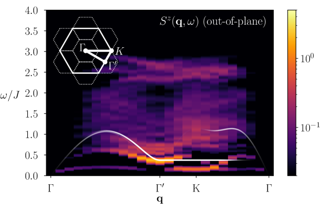
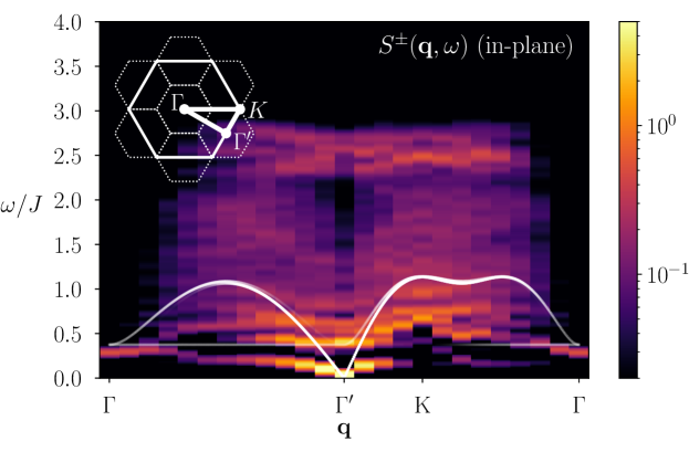
Figure 14: Out-of-plane [$S^{z}({\bf q},\omega)$, upper panel] and in-plane [$S^{\pm}({\bf q},\omega)$, lower panel] spin dynamical structure factor, for $J_{D}/J=0.05$. Calculations are performed on the $3\times 12\times 12$ cluster. LSW results for the three magnon modes are also shown for comparison (the intensity of the signal is proportional to the thickness of the white lines) [64]. The inset in the upper left corner of the figures shows the first and extended Brillouin zones of the kagome lattice (with dashed and solid lines, respectively), and the high symmetry points $\Gamma$ and $\Gamma^{\prime}$.

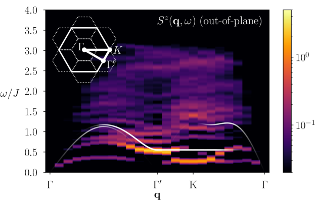
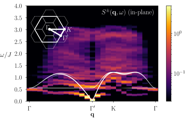
Figure 15: The same as in Fig. 14 for $J_{D}/J=0.1$.

References

- [1] J. Kosterlitz and D. Thouless, Ordering, metastability and phase transitions in two-dimensional systems, J. Phys. C: Solid State Phys. 6, 1181 (1973), 10.1088/0022-3719/6/7/010.
- [2] F. Haldane, Nonlinear Field Theory of Large-Spin Heisenberg Antiferromagnets: Semiclassically Quantized Solitons of the One-Dimensional Easy-Axis Néel State, Phys. Rev. Lett. 50, 1153 (1983), 10.1103/PhysRevLett.50.1153.
- [3] L. Savary and L. Balents, Quantum spin liquids: a review, Rep. Prog. Phys. 80, 016502 (2016), 10.1088/0034-4885/80/1/016502.
- [4] Y. Zhou, K. Kanoda and T.-K. Ng, Quantum spin liquid states, Rev. Mod. Phys. 89, 025003 (2017), 10.1103/RevModPhys.89.025003.
- [5] O. Motrunich, Variational study of triangular lattice spin-1/2 model with ring exchanges and spin liquid state in -(ET)2Cu2(CN)3, Phys. Rev. B 72, 045105 (2005), 10.1103/PhysRevB.72.045105.
- [6] A. Sandvik, Evidence for Deconfined Quantum Criticality in a Two-Dimensional Heisenberg Model with Four-Spin Interactions, Phys. Rev. Lett. 98, 227202 (2007), 10.1103/PhysRevLett.98.227202.
- [7] H.-Y. Yang, A. Läuchli, F. Mila and K. Schmidt, Effective Spin Model for the Spin-Liquid Phase of the Hubbard Model on the Triangular Lattice, Phys. Rev. Lett. 105, 267204 (2010), 10.1103/PhysRevLett.105.267204.
- [8] B. Bauer, L. Cincio, B. Keller, M. Dolfi, G. Vidal, S. Trebst and A. Ludwig, Chiral spin liquid and emergent anyons in a Kagome lattice Mott insulator, Nat. Commun. 5, 5137 (2014), 10.1038/ncomms6137.
- [9] W. Witczak-Krempa, G. Chen, Y. Kim and L. Balents, Correlated Quantum Phenomena in the Strong Spin-Orbit Regime, Annu. Rev. Condens. Matter Phys. 5, 57 (2014), 10.1146/annurev-conmatphys-020911-125138.
- [10] J. Rau, E.-H. Lee and H.-Y. Kee, Spin-Orbit Physics Giving Rise to Novel Phases in Correlated Systems: Iridates and Related Materials, Annu. Rev. Condens. Matter Phys. 7, 195 (2016), 10.1146/annurev-conmatphys-031115-011319.
- [11] K. Riedl, Y. Li, . Valentíand S. Winter, Ab Initio Approaches for Low-Energy Spin Hamiltonians, Phys. Status Solidi B 256(9), 1800684 (2019), https://doi.org/10.1002/pssb.201800684.
- [12] A. Kitaev, Anyons in an exactly solved model and beyond, Ann. Phys. 321(1), 2 (2006), https://doi.org/10.1016/j.aop.2005.10.005, January Special Issue.
- [13] I. Dzyaloshinsky, A thermodynamic theory of “weak” ferromagnetism of antiferromagnetics, J. Phys. Chem. Solids 4(4), 241 (1958), https://doi.org/10.1016/0022-3697(58)90076-3.
- [14] T. Moriya, Anisotropic Superexchange Interaction and Weak Ferromagnetism, Phys. Rev. 120, 91 (1960), 10.1103/PhysRev.120.91.
- [15] A. Olariu, P. Mendels, F. Bert, F. Duc, J. C. Trombe, M. A. de Vries and A. Harrison, NMR Study of the Intrinsic Magnetic Susceptibility and Spin Dynamics of the Quantum Kagome Antiferromagnet ZnCu3(OH)6Cl2, Phys. Rev. Lett. 100, 087202 (2008), 10.1103/PhysRevLett.100.087202.
- [16] T.-H. Han, J. Helton, S. Chu, D. Nocera, J. Rodriguez-Rivera, C. Broholm and Y. Lee, Fractionalized excitations in the spin-liquid state of a kagome-lattice antiferromagnet, Nature 492, 406 (2012), 10.1038/nature1165.
- [17] P. Khuntia, M. Velazquez, Q. Barthélemy, F. Bert, E. Kermarrec, A. Legros, B. Bernu, L. Messio, A. Zorko and P. Mendels, Gapless ground state in the archetypal quantum kagome antiferromagnet zncu3(oh)6cl2, Nature Physics 16(4), 469 (2020), 10.1038/s41567-020-0792-1.
- [18] J. Wang, W. Yuan, P. M. Singer, R. W. Smaha, W. He, J. Wen, Y. S. Lee and T. Imai, Emergence of spin singlets with inhomogeneous gaps in the kagome lattice heisenberg antiferromagnets zn-barlowite and herbertsmithite, Nature Physics 17(10), 1109 (2021), 10.1038/s41567-021-01310-3.
- [19] H. Jeschke, F. Salvat-Pujol and R. Valentí, First-principles determination of heisenberg hamiltonian parameters for the spin- kagome antiferromagnet zncu3(oh)6cl2, Phys. Rev. B 88, 075106 (2013), 10.1103/PhysRevB.88.075106.
- [20] A. Zorko, S. Nellutla, J. van Tol, L. Brunel, F. Bert, F. Duc, J.-C. Trombe, M. de Vries, A. Harrison and P. Mendels, Dzyaloshinsky-Moriya Anisotropy in the Spin-1/2 Kagome Compound ZnCu3(OH)6Cl2, Phys. Rev. Lett. 101, 026405 (2008), 10.1103/PhysRevLett.101.026405.
- [21] S. El Shawish, O. Cépas and S. Miyashita, Electron spin resonance in antiferromagnets at high temperature, Phys. Rev. B 81, 224421 (2010), 10.1103/PhysRevB.81.224421.
- [22] T. Arh, M. Gomilšek, P. Prelovšek, M. Pregelj, M. Klanjšek, A. Ozarowski, S. J. Clark, T. Lancaster, W. Sun, J.-X. Mi and A. Zorko, Origin of Magnetic Ordering in a Structurally Perfect Quantum Kagome Antiferromagnet, Phys. Rev. Lett. 125, 027203 (2020), 10.1103/PhysRevLett.125.027203.
- [23] M. Saito, R. Takagishi, N. Kurita, M. Watanabe, H. Tanaka, R. Nomura, Y. Fukumoto, K. Ikeuchi and R. Kajimoto, Structures of magnetic excitations in the spin- kagome-lattice antiferromagnets Cs2Cu3SnF12 and Rb2Cu3SnF12, Phys. Rev. B 105, 064424 (2022), 10.1103/PhysRevB.105.064424.
- [24] O. Cépas, C. Fong, P. Leung and C. Lhuillier, Quantum phase transition induced by Dzyaloshinskii-Moriya interactions in the kagome antiferromagnet, Phys. Rev. B 78, 140405 (2008), 10.1103/PhysRevB.78.140405.
- [25] M. Hering and J. Reuther, Functional renormalization group analysis of Dzyaloshinsky-Moriya and Heisenberg spin interactions on the kagome lattice, Phys. Rev. B 95, 054418 (2017), 10.1103/PhysRevB.95.054418.
- [26] C.-Y. Lee, B. Normand and Y.-J. Kao, Gapless spin liquid in the kagome Heisenberg antiferromagnet with Dzyaloshinskii-Moriya interactions, Phys. Rev. B 98, 224414 (2018), 10.1103/PhysRevB.98.224414.
- [27] Y. Iqbal, F. Becca, S. Sorella and D. Poilblanc, Gapless spin-liquid phase in the kagome spin- Heisenberg antiferromagnet, Phys. Rev. B 87, 060405 (2013), 10.1103/PhysRevB.87.060405.
- [28] H. Liao, Z. Xie, J. Chen, Z. Liu, H. Xie, R. Huang, B. Normand and T. Xiang, Gapless Spin-Liquid Ground State in the Kagome Antiferromagnet, Phys. Rev. Lett. 118, 137202 (2017), 10.1103/PhysRevLett.118.137202.
- [29] Y.-C. He, M. Zaletel, M. Oshikawa and F. Pollmann, Signatures of Dirac Cones in a DMRG Study of the Kagome Heisenberg Model, Phys. Rev. X 7, 031020 (2017), 10.1103/PhysRevX.7.031020.
- [30] L. Messio, O. Cépas and C. Lhuillier, Schwinger-boson approach to the kagome antiferromagnet with Dzyaloshinskii-Moriya interactions: Phase diagram and dynamical structure factors, Phys. Rev. B 81, 064428 (2010), 10.1103/PhysRevB.81.064428.
- [31] Y. Huh, L. Fritz and S. Sachdev, Quantum criticality of the kagome antiferromagnet with Dzyaloshinskii-Moriya interactions, Phys. Rev. B 81, 144432 (2010), 10.1103/PhysRevB.81.144432.
- [32] T. Dodds, S. Bhattacharjee and Y. Kim, Quantum spin liquids in the absence of spin-rotation symmetry: Application to herbertsmithite, Phys. Rev. B 88, 224413 (2013), 10.1103/PhysRevB.88.224413.
- [33] S. Bieri, C. Lhuillier and L. Messio, Projective symmetry group classification of chiral spin liquids, Phys. Rev. B 93, 094437 (2016), 10.1103/PhysRevB.93.094437.
- [34] L. Messio, S. Bieri, C. Lhuillier and B. Bernu, Chiral Spin Liquid on a Kagome Antiferromagnet Induced by the Dzyaloshinskii-Moriya Interaction, Phys. Rev. Lett. 118, 267201 (2017), 10.1103/PhysRevLett.118.267201.
- [35] P. Prelovšek, M. Gomilšek, T. Arh and A. Zorko, Dynamical spin correlations of the kagome antiferromagnet, Phys. Rev. B 103, 014431 (2021), 10.1103/PhysRevB.103.014431.
- [36] W. Zhu, S.-S. Gong and D. Sheng, Identifying spinon excitations from dynamic structure factor of spin-1/2 heisenberg antiferromagnet on the kagome lattice, Proceedings of the National Academy of Sciences 116(12), 5437 (2019), 10.1073/pnas.1807840116.
- [37] C. Gros, Physics of projected wavefunctions, Ann. Phys. 189(1), 53 (1989), https://doi.org/10.1016/0003-4916(89)90077-8.
- [38] F. Verstraete, V. Murg and J. Cirac, Matrix product states, projected entangled pair states, and variational renormalization group methods for quantum spin systems, Adv. Phys. 57(2), 143 (2008), 10.1080/14789940801912366.
- [39] N. Schuch, D. Poilblanc, J. Cirac and D. Pérez-García, Resonating valence bond states in the PEPS formalism, Phys. Rev. B 86, 115108 (2012), 10.1103/PhysRevB.86.115108.
- [40] Z. Xie, J. Chen, J. Yu, X. Kong, B. Normand and T. Xiang, Tensor Renormalization of Quantum Many-Body Systems Using Projected Entangled Simplex States, Phys. Rev. X 4, 011025 (2014), 10.1103/PhysRevX.4.011025.
- [41] H.-J. Liao, J.-G. Liu, L. Wang and T. Xiang, Differentiable Programming Tensor Networks, Phys. Rev. X 9, 031041 (2019), 10.1103/PhysRevX.9.031041.
- [42] M. Rader and A. Läuchli, Finite Correlation Length Scaling in Lorentz-Invariant Gapless iPEPS Wave Functions, Phys. Rev. X 8, 031030 (2018), 10.1103/PhysRevX.8.031030.
- [43] P. Corboz, P. Czarnik, G. Kapteijns and L. Tagliacozzo, Finite Correlation Length Scaling with Infinite Projected Entangled-Pair States, Phys. Rev. X 8, 031031 (2018), 10.1103/PhysRevX.8.031031.
- [44] T. Li and F. Yang, Variational study of the neutron resonance mode in the cuprate superconductors, Phys. Rev. B 81, 214509 (2010), 10.1103/PhysRevB.81.214509.
- [45] B. Dalla Piazza, M. Mourigal, N. Christensen, G. Nilsen, P. Tregenna-Piggott, T. Perring, M. Enderle, D. McMorrow, D. Ivanov and H. Rønnow, Fractional excitations in the square-lattice quantum antiferromagnet, Nat. Phys. 11(1), 62 (2015), 10.1038/nphys3172.
- [46] F. Ferrari and F. Becca, Spectral signatures of fractionalization in the frustrated Heisenberg model on the square lattice, Phys. Rev. B 98, 100405 (2018), 10.1103/PhysRevB.98.100405.
- [47] F. Ferrari and F. Becca, Dynamical Structure Factor of the Heisenberg Model on the Triangular Lattice: Magnons, Spinons, and Gauge Fields, Phys. Rev. X 9, 031026 (2019), 10.1103/PhysRevX.9.031026.
- [48] F. Ferrari and F. Becca, Dynamical properties of Néel and valence-bond phases in the model on the honeycomb lattice, J. Phys. Condens. Matter 32, 274003 (2020), 10.1088/1361-648X/ab7f6e.
- [49] C. Zhang and T. Li, Variational study of the ground state and spin dynamics of the spin- kagome antiferromagnetic Heisenberg model and its implication for herbertsmithite , Phys. Rev. B 102, 195106 (2020), 10.1103/PhysRevB.102.195106.
- [50] F. Ferrari, A. Parola and F. Becca, Gapless spin liquids in disguise, Phys. Rev. B 103, 195140 (2021), 10.1103/PhysRevB.103.195140.
- [51] D. Vörös and K. Penc, Dynamical structure factor of the SU(3) Heisenberg chain: Variational Monte Carlo approach, Phys. Rev. B 104, 184426 (2021), 10.1103/PhysRevB.104.184426.
- [52] P. Corboz, T. Rice and M. Troyer, Competing States in the - Model: Uniform -Wave State versus Stripe State, Phys. Rev. Lett. 113, 046402 (2014), 10.1103/PhysRevLett.113.046402.
- [53] J. Hasik and G. Mbeng, peps-torch: A differentiable tensor network library for two-dimensional lattice models, https://github.com/jurajHasik/peps-torch.
- [54] Y. Iqbal, F. Becca and D. Poilblanc, Projected wave function study of spin liquids on the kagome lattice for the spin- quantum Heisenberg antiferromagnet, Phys. Rev. B 84, 020407 (2011), 10.1103/PhysRevB.84.020407.
- [55] Y. Iqbal, D. Poilblanc, R. Thomale and F. Becca, Persistence of the gapless spin liquid in the breathing kagome Heisenberg antiferromagnet, Phys. Rev. B 97, 115127 (2018), 10.1103/PhysRevB.97.115127.
- [56] Y. Iqbal, F. Ferrari, A. Chauhan, A. Parola, D. Poilblanc and F. Becca, Gutzwiller projected states for the Heisenberg model on the Kagome lattice: Achievements and pitfalls, Phys. Rev. B 104, 144406 (2021), 10.1103/PhysRevB.104.144406.
- [57] G. Baskaran and P. Anderson, Gauge theory of high-temperature superconductors and strongly correlated Fermi systems, Phys. Rev. B 37, 580 (1988), 10.1103/PhysRevB.37.580.
- [58] I. Affleck and J. Marston, Large-n limit of the Heisenberg-Hubbard model: Implications for high- superconductors, Phys. Rev. B 37, 3774 (1988), 10.1103/PhysRevB.37.3774.
- [59] I. Affleck, Z. Zou, T. Hsu and P. Anderson, SU(2) gauge symmetry of the large- limit of the Hubbard model, Phys. Rev. B 38, 745 (1988), 10.1103/PhysRevB.38.745.
- [60] M. Hastings, Dirac structure, RVB, and Goldstone modes in the kagomé antiferromagnet, Phys. Rev. B 63, 014413 (2000), 10.1103/PhysRevB.63.014413.
- [61] Y. Ran, M. Hermele, P. Lee and X.-G. Wen, Projected-Wave-Function Study of the Spin- Heisenberg Model on the Kagomé Lattice, Phys. Rev. Lett. 98, 117205 (2007), 10.1103/PhysRevLett.98.117205.
- [62] H. Neuberger and T. Ziman, Finite-size effects in Heisenberg antiferromagnets, Phys. Rev. B 39, 2608 (1989), 10.1103/PhysRevB.39.2608.
- [63] D. Fisher, Universality, low-temperature properties, and finite-size scaling in quantum antiferromagnets, Phys. Rev. B 39, 11783 (1989), 10.1103/PhysRevB.39.11783.
- [64] S. Toth and B. Lake, Linear spin wave theory for single-Q incommensurate magnetic structures, J. Phys. Condens. Matter 27(16), 166002 (2015), 10.1088/0953-8984/27/16/166002.
- [65] F. Franjić and S. Sorella, Spin-Wave Wave Function for Quantum Spin Models, Prog. Theor. Phys. 97(3), 399 (1997), 10.1143/PTP.97.399.
- [66] T. Ono, K. Matan, Y. Nambu, T. Sato, K. Katayama, S. Hirata and H. Tanaka, Large Negative Quantum Renormalization of Excitation Energies in the Spin-1/2 Kagome Lattice Antiferromagnet Cs2Cu3SnF12, J. Phys. Soc. Japan 83(4), 043701 (2014), 10.7566/JPSJ.83.043701.