IDET: Iterative Difference-Enhanced Transformers for High-Quality Change Detection

Abstract

Change detection (CD) aims to detect change regions within an image pair captured at different times, playing a significant role in diverse real-world applications. Nevertheless, most of the existing works focus on designing advanced network architectures to map the feature difference to the final change map while ignoring the influence of the quality of the feature difference. In this paper, we study the CD from a different perspective, i.e., how to optimize the feature difference to highlight changes and suppress unchanged regions, and propose a novel module denoted as iterative difference-enhanced transformers (IDET). IDET contains three transformers: two transformers for extracting the long-range information of the two images and one transformer for enhancing the feature difference. In contrast to the previous transformers, the third transformer takes the outputs of the first two transformers to guide the enhancement of the feature difference iteratively. To achieve more effective refinement, we further propose the multi-scale IDET-based change detection that uses multi-scale representations of the images for multiple feature difference refinements and proposes a coarse-to-fine fusion strategy to combine all refinements. Our final CD method outperforms seven state-of-the-art methods on six large-scale datasets under diverse application scenarios, which demonstrates the importance of feature difference enhancements and the effectiveness of IDET.

I Introduction

Change detection (CD) aims to detect change areas caused by object variations (e.g., new objects appear in the scene) from an image pair captured at different times, which has wide applications in urban development [1], disaster assessment [2], resource monitoring, and utilization [3, 4, 5], abandoned object detection [6], illegally parked vehicles [7] and military [8, 9]. Change detection is challenging since the two images are captured at different angles and illuminations, and the scenes have unknown changes in the background. As the case in Fig. 1 (b), the color of the sky and the intensity of buildings vary dramatically within the two images, which, however, should not be identified as changes.

A straightforward idea is to calculate the differences between the features of the two images and map the feature difference to the final change map [10, 11]. The features and feature differences are desired to conquer the environment variation and position misalignment. A representative work [10] proposes cross-encoded features to calculate the feature differences of an image pair and generate a change map. FPIN [12] uses a complex feature extraction network (i.e., fluid pyramid integration network [13]) to improve the CD accuracy by improving feature representational capability. Another work [11] proposes position-correlated attention, channel-correlated attention and change difference modules to capture the correlation of the two images. The above state-of-the-art (SOTA) methods focus on designing advanced network architectures to map the feature difference to the final change map. Although achieving impressive detection accuracy, these methods ignore the influence of the quality of the feature difference. Intuitively, if the feature difference could clearly highlight the main changes while suppressing unchanged regions, we are able to achieve high-quality change maps more easily. As the cases shown in Fig. 1, when the feature difference (i.e., $\mathbf{D}$) is corrupted (e.g., noisy feature difference in Fig. 1 (b) and (c)), the detection results decrease significantly. Note that, the quality of feature difference may be affected by diverse environment variations like light or weather changes.

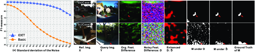
Figure 1: (a) Evaluation results on the VL-CMU-CD dataset by adding noise with different severities to the feature difference $\mathbf{D}$. (b) and (c) display two cases including the original feature difference, noisy feature difference $\mathbf{D}$, enhanced feature difference $\hat{\mathbf{D}}$, the detection results $\mathbf{M}$ under $\mathbf{D}$ and $\hat{\mathbf{D}}$, and the ground truth, respectively. The main changes are highlighted via red arrows.

To fill this gap, we study change detection from a different angle, i.e., how to optimize the feature difference to highlight main changes and suppress unchanged regions, and propose a novel module denoted as iterative difference-enhanced transformers (IDET). IDET contains three transformers, the first two transformers are to extract the global information of the two input images while the third transformer is to enhance the feature differences. Note that, the third transformer is different from existing transformers, taking the outputs of the first two transformers to guide the feature difference refinement iteratively. Then, we fuse these refinements for high-quality detection via a coarse-to-fine method. Overall, our contributions can be summarized as follows:

• We build a basic feature difference-based CD method and study the influence of feature difference quality on detection accuracy by adding random noise with different severities. The analysis infers that the feature difference quality is critical to high-quality detection.

• We propose an iterative difference-enhanced transformer (IDET) to refine the feature difference by extracting the long-range information within inputs as guidance. We further extend a multi-scale IDET with multi-scale representations and a coarse-to-fine fusion strategy.

• We perform extensive experiments on six datasets covering a wide range of scenarios, resolutions, and change ratios. Our method outperforms seven state-of-the-art methods.

II Related Work

Change detection methods. According to different applications, CD methods can be divided into two types: CD for common scenarios and remote sensing. Both types retrieve changes from an image pair. The main differences stem from the image resolutions and the size of the change regions.

CD methods for common scenarios [14, 12] use images captured by consumer cameras, and the results are affected by camera pose misalignment and illumination difference easily. The input images for remote sensing CD methods contain high-resolution remote sensing images [15, 16], hyperspectral images [17], SAR images [18], etc. However, the changes are usually subtle. Early works have demonstrated the effectiveness of principal component analysis (PCA) [19] and change vector analysis (CVA) [20] for CD. With the development of deep neural networks, recent methods also adopt deep neural networks as the mainstream solution. FPIN [12] employs different fluid pyramid integration networks to fuse multi-level features. Dual correlation attention modules are utilized to refine the change features on the same scale [11].

However, these works mainly focus on designing novel deep models. In contrast, we focus on a new problem, i.e., the influence of feature difference quality. With extensive study, we propose a feature difference enhancement method outperforming SOTA methods on diverse applications including the common and remote sensing scenarios.

Transformer for vision tasks. The transformer has been widely used in most natural language processing (NLP) tasks for its long-range dependency since it was proposed in [21]. Recently, the transformer has shown promising performance in computer vision tasks, such as image classification [22, 23, 24], object detection [25, 26, 27], semantic segmentation [28, 29, 30, 31], and crowd counting [32, 23]. The excellent performance of transformer models inspires us to study their application in CD. Till now, there are few works using the transformer for CD tasks. BiT [33] agrees that the transformer encoder can model the semantic information of change objects to refine the coarse change maps predicted by the decoder. However, it is difficult to learn the semantic tokens when the changed objects are small and diverse. ChangeFormer [34] is composed of a series of hierarchically structured transformer encoders for extracting the long-range features to generate change masks. Due to the low resolutions of its encoders, which can not capture the detailed changes at the boundary.

In contrast to BiT [33] and ChangeFormer [34], our work has totally different objectives and architecture. Specifically, the proposed module contains three transformers with a novel designed transformer for effective feature difference refinement.

III Feature Difference-based CD and Motivation

In this section, we first introduce a lightweight convolutional neural network, the basic feature difference-based CD model, and then analyze the issues from the viewpoint of the feature difference quality.

III-A Feature Difference-based CD

Given a reference image $\mathbf{X}$ and a query image $\mathbf{Y}$, a change detector $\phi(\cdot)$ takes the two images as the input and predicts a change map $\mathbf{M}$ that indicates changing regions between the two images, which are caused by object variations (e.g., new objects appearing in the scene) instead of the environment changes (e.g., light variations). We can represent the whole process as $\mathbf{M}=\phi(\mathbf{X},\mathbf{Y})$. The main challenge is how to distinguish the object changes from environmental variations. Previous works calculate the difference between the features of $\mathbf{X}$ and $\mathbf{Y}$ explicitly and map it to the final change mask, which is robust to diverse environment variations [10]. We follow the feature difference solution and build the basic change detection method via a CNN. Specifically, we feed $\mathbf{X}$ or $\mathbf{Y}$ to the CNN and get a series of features $\{\mathbf{F}^{l}_{\text{x}~{}\text{or}~{}\text{y}}\}_{l=1}^{L}$. Then, we can calculate the feature difference at each layer $l$ and fuse them by a convolution layer

$$\mathbf{D}=\text{Fuse}(\{\mathbf{D}^{l}\}_{l=1}^{L}),~{}\forall~{}l~{},\mathbf{D}^{l}=|\mathbf{F}^{l}_{\text{x}}-\mathbf{F}^{l}_{\text{y}}|,$$ (1)

where the feature difference $\mathbf{D}$ can be fed to the other two convolution layers to predict the final change map $\mathbf{M}$. We present all architecture details in Fig. 2. Previous works mainly design more advanced architecture to replace the basic CNN [35]. In contrast, we focus on the influence of the quality of $\mathbf{D}$, which is not explored yet.

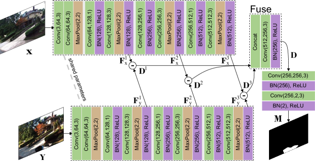
Figure 2: Architecture of feature difference-based change detection.

III-B Analysis and Motivation

Based on Fig. 2, we study the importance of the quality of $\mathbf{D}$ to the final change map. Given an image pair from VL-CMU-CD dataset  [36] (e.g., Fig. 1 (b) and (c)), we feed them to Eq. (1) and get the original feature difference denoted as $\mathbf{D}_{\text{o}}$. Then, we add random noise to the unchanged regions of $\mathbf{D}_{\text{o}}$ to simulate the feature difference with diverse qualities. Specifically, according to the ground truth of the change regions, we first calculate the averages of feature difference values inside and outside change regions, which are denoted as $d_{\text{o}}^{\text{inside}}$ and $d_{\text{o}}^{\text{outside}}$, respectively. Then, we set a zero-mean random noise with standard deviation as $\alpha|d_{\text{o}}^{\text{inside}}-d_{\text{o}}^{\text{outside}}|$ and add the noise to the unchanged regions in $\mathbf{D}_{\text{o}}$ to get a degraded version denoted as $\mathbf{D}$. We can conduct this process for all examples with the $\alpha$ from 5 to 100 with the interval of 5. Then, for each $\alpha$, we can evaluate the detection results via the F1-measure. According to the dark orange stars in Fig. 1 (a), we see that the basic CD method is very sensitive to the quality of the feature difference. Clearly, as the noise becomes larger, the F1 value decreases significantly. We have a similar conclusion on the visualization results in Fig. 1: the low-quality feature difference leads to incorrect detection.

IV Methodology

IV-A Problem Definition and Challenges

Due to the importance of feature difference quality, we formulate the feature difference enhancement as a novel task: given the representations of $\mathbf{X}$ and $\mathbf{Y}$ (i.e., $\mathbf{R}_{\text{x}}$ and $\mathbf{R}_{\text{y}}$) and an initialized feature difference $\mathbf{D}$, we aim to refine $\mathbf{D}$ and get a better one (i.e., $\hat{\mathbf{D}}$) where the object changes are highlighted and other distractions are suppressed.

The feature difference enhancement is a non-trivial task since pixel changes between $\mathbf{X}$ and $\mathbf{Y}$ stem from the object and environment changes and it is difficult to distinguish the changes from each other. To achieve this refinement, a feature difference enhancement method should first understand the whole scene in both reference and query images and know which regions are caused by object changes. Moreover, the extracted discriminative information should be effectively embedded into the initial feature difference $\mathbf{D}$ to guide the refinement.

IV-B Iterative Difference-enhanced Transformers

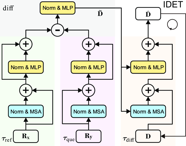
Figure 3: Architecture of Iterative Difference-enhanced Transformers (IDET).

Overview. We employ the transformer to achieve the feature difference enhancement due to the impressive improvements of transformer-based methods in diverse vision tasks [24, 31]. Note that, the transformer is able to capture the long-term dependency of the whole inputs, which meets the requirements of the feature difference enhancement. Nevertheless, how to adapt such an advanced technique to the new task is not clear. To this end, we propose the iterative difference-enhanced transformers (IDET) for feature difference enhancement.

IDET contains three transformers, i.e., reference transformer $\tau_{\text{ref}}(\cdot)$, query transformer $\tau_{\text{que}}(\cdot)$, and difference refinement transformer $\tau_{\text{diff}}(\cdot)$. The whole process of IDET is shown in Fig. 3 and can be formulated as:

$$\hat{\mathbf{D}}=\tau_{\text{diff}}(\mathbf{D},\tilde{\mathbf{D}}),~{}\text{with}~{}\tilde{\mathbf{D}}=\text{diff}(\tau_{\text{ref}}(\mathbf{R}_{\text{x}}),\tau_{\text{que}}(\mathbf{R}_{\text{y}})),$$ (2)

where the transformers $\tau_{\text{ref}}(\cdot)$ and $\tau_{\text{que}}(\cdot)$ are employed to extract the long-range information in $\mathbf{X}$ and $\mathbf{Y}$, respectively, while the function $\text{diff}(\tau_{\text{ref}}(\mathbf{R}_{\text{x}}),\tau_{\text{que}}(\mathbf{R}_{\text{y}}))$ is

$$\begin{split}\tilde{\mathbf{D}}&=\text{diff}(\tau_{\text{ref}}(\mathbf{R}_{\text{x}}),\tau_{\text{que}}(\mathbf{R}_{\text{y}}))\\ &=\text{MLP}(\text{Norm}(|\tau_{\text{ref}}(\mathbf{R}_{\text{x}})-\tau_{\text{que}}(\mathbf{R}_{\text{y}}|))).\end{split}$$ (3)

It aims to generate difference information (i.e., $\tilde{\mathbf{D}}$) from the two long-range features (i.e., $\tau_{\text{ref}}(\mathbf{R}_{\text{x}})$ and $\tau_{\text{que}}(\mathbf{R}_{\text{y}})$) through a multilayer perceptron (MLP) and a layer norm (Norm). Finally, the $\tilde{\mathbf{D}}$ is fed to the difference refinement transformer (i.e., $\tau_{\text{diff}}(\cdot)$) to guide the updating of the initial $\mathbf{D}$. Moreover, we can make the output $\hat{\mathbf{D}}$ as the initial feature difference and refine it again and again. As a result, the method becomes iterative. We show the whole architecture in Fig. 3 and detail them in the following subsections.

Architectures of $\tau_{\text{ref}}(\cdot)$ and $\tau_{\text{que}}(\cdot)$. We eliminate the position token and class token in the model designation because we don’t use patch embedding and ignore the object labels. The whole process can be formulated as

$$\begin{split}\tau_{*}(\mathbf{R}_{*})&=\text{MLP}(\text{Norm}(\mathbf{Z}))+\mathbf{Z},~{}\text{with}~{}\\ \mathbf{Z}&=\text{MSA}(\text{Norm}(\mathbf{R}_{*}))+\mathbf{R}_{*},\end{split}$$ (4)

where $\text{MSA}(\cdot)$ is the efficient multi-head self-attention introduced in [31].

Architecture of $\tau_{\text{diff}}(\cdot)$. In contrast to the above transformers, $\tau_{\text{diff}}(\cdot)$ uses the difference information $\tilde{\mathbf{D}}$ obtained by Eq. (3) to guide the refinement of the initial $\mathbf{D}$. To this end, we modify the Eq. (4) by

$$\begin{split}\tau_{\text{diff}}(\mathbf{D},\tilde{\mathbf{D}})&=\text{MLP}(\text{Norm}(\tilde{\mathbf{D}}))+\mathbf{Z},~{}\text{with}~{}\\ \mathbf{Z}&=\text{MSA}(\text{Norm}(\tilde{\mathbf{D}}))+\mathbf{D}.\end{split}$$ (5)

The intuitive idea is to use MSA and MLP to extract the long-term information in $\tilde{\mathbf{D}}$ and embed it to update $\mathbf{D}$.

IV-C Multi-scale IDET-based CD

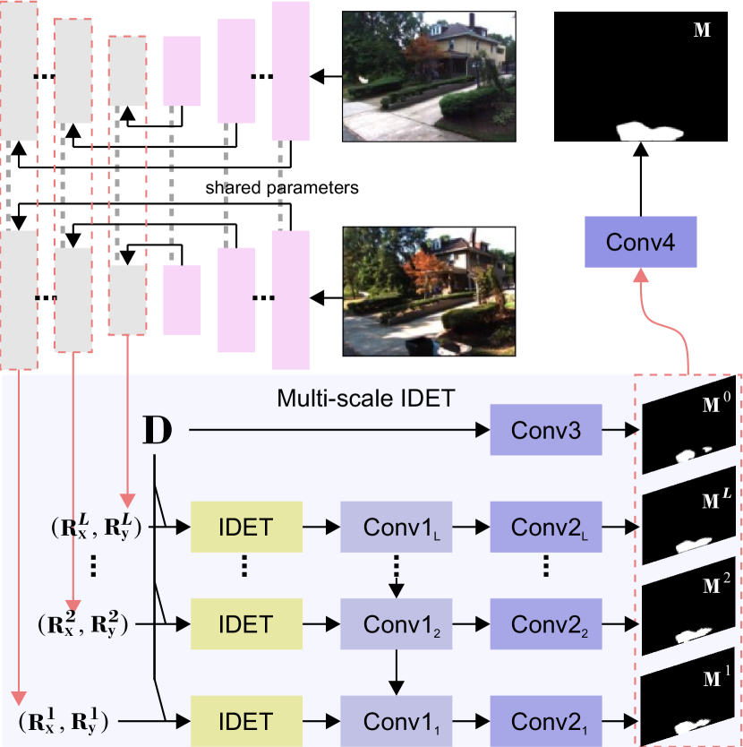
Figure 4: Multi-scale IDET-based change detection.

With the proposed IDET, we are able to update the basic feature difference-based CD introduced in above. The key problem is how to select the representations (i.e., $\mathbf{R}_{\text{x}}$ and $\mathbf{R}_{\text{y}}$ in Eq. (2)) to refine the feature difference $\mathbf{D}$ in Eq. (1) and how to fuse refined results from different representations. Here, we propose to use UNet [37] to extract multi-scale convolutional features as the representations and can get a refined feature difference for each scale, and then design a coarse-to-fine fusion method to combine multi-scale results. Specifically, given a UNet containing an encoder and a decoder, we feed $\mathbf{X}$ and $\mathbf{Y}$ to the network, respectively, and get multi-scale representations from all the layers of the decoder, which are denoted as $\{\mathbf{R}^{l}_{\text{x}}\}^{L}$ and $\{\mathbf{R}^{l}_{\text{y}}\}^{L}$ where $L$ denotes the number of scales. Note that, given $\mathbf{R}^{l}_{\text{x}}$, and $\mathbf{R}^{l}_{\text{y}}$, we still cannot refine $\mathbf{D}$ through the IDET directly since $\mathbf{D}$ from Eq. (1) has smaller resolution than $\mathbf{R}^{l}_{\text{x}}$ and $\mathbf{R}^{l}_{\text{y}}$. To use IDET at the scale $l$, we upsample $\mathbf{D}$ to the size of $\mathbf{R}^{l}_{\text{x}}$ and $\mathbf{R}^{l}_{\text{y}}$ and get a refined result $\hat{\mathbf{D}}^{l}$. For all scales, we have $\{\hat{\mathbf{D}}^{l}\}_{l=1}^{L}$ and fuse them via a coarse-to-fine strategy, i.e.,

$$\hat{\mathbf{D}}^{\prime l}=\text{Conv1}_{l}([\hat{\mathbf{D}}^{l},\hat{\mathbf{D}}^{\prime(l-1)}]),~{}\text{with}~{}l=1,\ldots,L,$$ (6)

where ‘$[\cdot]$’ denotes the concatenation operation and $~{}\hat{\mathbf{D}}^{\prime 0}=\text{empty}$. For $\hat{\mathbf{D}}^{\prime l}$ and the initial $\mathbf{D}$, we use a convolution layer to extract a change map

$$\mathbf{M}^{l}=\text{Conv2}_{l}(\hat{\mathbf{D}}^{\prime l}),~{}\text{and}~{}\mathbf{M}^{0}=\text{Conv3}(\mathbf{D}).$$ (7)

Then, the final output is obtained via $\mathbf{M}=\text{Conv4}([\mathbf{M}^{0},\ldots,\mathbf{M}^{L}]).$

IV-D Implementation Details

Architecture of UNet. As shown in Fig. 2, we conduct our UNet implementation. It has five squeeze modules to extract abstract features by reducing the spatial resolution and five expanded modules to restore the resolution of the features by incorporating high-resolution and low-level features from squeeze modules.

Setups of Conv* for fusion. $\text{Conv1}_{*}(\cdot)$ in Eq. (6) contains three modules, each of which has a convolutional layer and a ReLU layer. The first convolution is responsible for reducing the channel number to half of the channel number of the input feature. The second convolution has the same input and output channel number to further refine the feature. The third convolution produces a feature with a given output channel number. The filter size in convolutions are $3\times 3$. $\text{Conv2}_{*}(\cdot)$ in Eq. (7) is a convolutional layer with the size of $N\times 3\times 3\times 2$, where $N$ represents the input channel number. $\text{Conv3}(\cdot)$ is used to generate change map $\mathbf{M}^{0}$ from the feature difference $\mathbf{D}$. $\text{Conv4}(\cdot)$ consists of $12\times 3\times 3\times 2$ convolutional filters to generate final change map $\mathbf{M}$.

Loss functions. Given a prediction $\mathbf{M}^{*}$ and the ground truth, we can calculate the cross-entropy loss denoted as $\mathcal{L}_{\mathbf{M}^{*}}$. We employ the cross-entropy loss on all the predicted change maps of $\mathbf{M}^{0},\ldots,\mathbf{M}^{L}$ and $\mathbf{M}$, and get a total loss:

$$\mathcal{L}=\sum_{l=1}^{L}\mathcal{L}_{\mathbf{M}^{l}}+\mathcal{L}_{\mathbf{M}}.$$ (8)

Training parameters. Our model is implemented on PyTorch [38] and trained with a single NVIDIA Geforce 2080Ti GPU. The basic learning rate is set to 1e-3. We set the batch size to 4. The parameters are updated by Adam algorithm with a momentum of 0.9 and weight decay of 0.999. Note that we use the same training parameters for all six datasets. Following [39], we train all CD methods with 20 and 200 epochs for common scene datasets and remote sensing datasets, respectively.

TABLE I: Dataset details. The change ratio is the proportion of the number of changed pixels to the total number of pixels.

	VL-CMU-CD	PCD	CDnet	LEVIR-CD	CDD	AICD
Image number	1362	200	50209	637	11	1000
Resolution	$1024\times 768$	$1024\times 224$	$320\times 240$,	$1024\times 1024$	$4725\times 2700$	$800\times 600$
			$720\times 576$		$1900\times 1000$
Categories	bins, signs, maintenance, vehicles, etc.	trees, buildings, vehicles, etc.	person, vehicles, boats, etc.	buildings	buildings, vehicles, roads, etc.	pavilions, ships etc.
Change ratio	0.0716	0.2587	0.0479	0.1116	0.1234	0.0022
Training image number	16005	8000	40148	18015	12998	25074
Testing image number	332	120	10061	4674	3000	464
Training image size	$320\times 320$	$320\times 320$	$320\times 320$	$256\times 256$	$256\times 256$	$256\times 256$

TABLE II: Quantitative comparison of CD methods on VL-CMU-CD, PCD and CDnet. The bold is the best.

Method	VL-CMU-CD					PCD					CDnet
	P	R	F1	OA	IoU	P	R	F1	OA	IoU	P	R	F1	OA	IoU
FCNCD	84.2	84.3	84.2	98.4	72.9	68.7	61.7	65.0	94.1	48.0	82.9	88.3	85.5	99.2	76.0
ADCDnet	92.8	94.3	93.5	99.3	87.9	78.8	73.4	76.0	90.0	62.3	89.0	85.5	87.2	99.3	77.9
CSCDnet	89.2	91.1	90.1	98.7	82.1	66.0	72.6	69.1	83.7	51.9	93.9	82.3	87.7	99.0	78.4
IFN	93.1	75.9	83.6	98.1	71.4	69.5	75.7	72.5	87.2	57.7	93.1	80.0	86.1	98.9	75.3
BIT	90.5	87.6	89.0	98.8	80.6	77.7	57.3	66.0	85.4	50.1	95.4	81.9	88.1	99.1	78.9
STAnet	73.1	95.8	82.9	98.0	70.7	69.6	52.7	60.0	79.9	41.2	72.2	94.3	81.8	98.3	69.2
ChangeFormer	88.0	88.6	88.3	98.7	79.2	74.0	69.2	71.5	86.6	56.4	93.4	85.9	89.5	99.2	81.3
IDET (Ours)	93.5	94.5	94.0	99.4	88.7	74.2	77.9	76.0	88.8	61.9	90.8	94.1	92.4	99.7	86.2

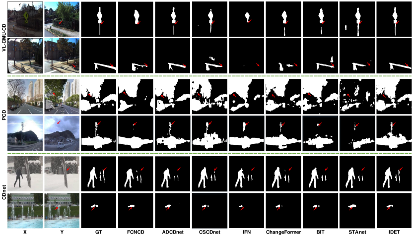
Figure 5: Detection results of different CD methods on VL-CMU-CD [36], PCD [40] and CDnet [41] datasets.

V Experiments

V-A Setup

Baselines. We compare our method with seven CD methods, i.e., FCNCD [42], ADCDnet [10], CSCDnet [43], BIT [33], IFN [35], STAnet [39] and ChangeFormer [34]. All compared methods are trained under the same setup.

TABLE III: Quantitative comparison of CD methods on LEVIR-CD, CDD and AICD. The bold is the best.

Method	LEVIR-CD					CDD					AICD
	P	R	F1	OA	IoU	P	R	F1	OA	IoU	P	R	F1	OA	IoU
FCNCD	89.7	84.0	86.8	97.7	77.1	85.1	69.8	76.7	97.5	63.7	81.4	87.7	84.4	99.9	72.7
ADCDnet	90.4	81.8	85.9	97.4	75.4	92.5	78.8	85.1	98.5	75.1	85.0	99.0	91.5	99.9	84.2
CSCDnet	84.6	81.6	83.1	96.8	71.5	79.1	48.9	60.4	90.9	42.7	92.5	88.9	90.7	99.9	82.6
IFN	89.7	79.8	84.5	96.9	72.7	94.2	69.2	79.8	97.7	66.5	84.6	97.7	90.7	99.9	82.9
BIT	92.1	81.6	86.5	97.7	76.3	93.5	80.2	86.3	98.7	76.6	94.2	92.4	93.2	99.9	87.4
STAnet	84.8	69.9	76.6	95.3	61.8	71.6	69.6	70.6	95.0	54.6	46.0	35.6	40.1	99.4	22.4
ChangeFormer	90.7	85.5	88.0	98.0	79.0	89.2	73.0	80.3	98.0	68.0	82.7	98.3	89.8	99.9	81.5
IDET (Ours)	91.3	86.6	88.9	98.1	80.2	91.1	83.1	86.9	98.7	77.6	96.2	90.4	93.2	99.9	87.2

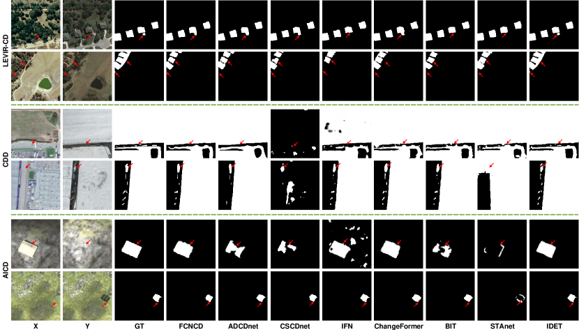
Figure 6: Detection results of different CD methods on LEVIR-CD [39], CDD [44] and AICD [45] datasets.

Datasets. We conduct experiments on three common-sense CD datasets, i.e., VL-CMU-CD [36], PCD [40] and CDnet [41], and three remote sensing CD datasets, i.e., LEVIR-CD [39], CDD [44] and AICD [45]. For VL-CMU-CD [36], we randomly select 80% image pairs for training and 20% for testing. The training images are augmented by randomly clipping and flipping. For PCD [40], we crop the image with a size of $224\times 224$, and partition the training and testing set with a ratio of 8:2. The training images are flipped to increase the number of training images. For CDnet [41], we use the training and testing dataset as proposed [10]. For LEVIR-CD [39], we crop images into small patches of size 256 × 256 without overlapping and augment training images with rotation and color transformation. Finally, we obtain 15835 and 4675 image pairs for training and testing, respectively. For CDD [44], we crop and rotate the original images to generate 10000 training and 3000 testing image pairs as proposed in [44]. For AICD [45], we crop image pairs randomly and augment the training images by rotation and color vibration. The details of these datasets are shown in Table. I.

Evaluation metrics. Following [33], we use precision (P), recall (R), F1-measure (F1), overall accuracy (OA) and intersection over union (IoU) to evaluate different CD methods, which can be calculated as:

$$P =\frac{TP}{TP+FP},$$ (9)

$$R =\frac{TP}{TP+FN},$$

$$F1 =\frac{2\times P\times R}{P+R},$$

$$OA =\frac{TP+TN}{TP+TN+FP+FN},$$

$$IoU =\frac{TP}{TP+FP+FN}$$

where $TP$, $TN$, $FP$ and $FN$, represent true positive, true negative, false positive, false negative, respectively.

V-B Comparison Result

Qualitative results analysis. Fig. 5 shows some representative CD examples of the state-of-the-art methods on VL-CMU-CD, PCD, and CDnet datasets. FCNCD [42] only captures the main parts of changes, which loses the details of the changes as shown in the 1st to 4th rows of Fig. 5. As illustrated in the 2nd and 3rd rows of Fig. 5, CSCDnet [43] is a weakness to detect changes in lighting difference scenes. IFN [35] also loses the detailed information of changes, even loses the change object in the 2nd row of Fig. 5. Transformer-based methods ChangeFormer [34] and BIT [33] are all easily affected by shadows and background clusters, which results in false detection in the 2nd and 4th rows of Fig. 5. STAnet [39] generates incomplete CD results as shown in the 4th and 5th rows of Fig. 5. Among the compared methods, ADCDnet [10] gains good CD results on all three CD datasets. However, we can find that the results of IDET are more complete and have more details as shown in the last column of Fig. 5.

Fig. 6 shows some typical detection results of different CD methods on LEVIR-CD, CDD and AICD datasets. IFN [35], BIT [33] and STAnet [39] fail to detect the small house in the 1st row of Fig. 6. In the 2nd row of Fig. 6, only IDET can detect the connected changes. CSCDnet [43] achieves the worst result on the CDD dataset, in the 3rd and 4th rows of Fig. 6, which demonstrates that CSCDnet cannot deal with the large changes. ADCDnet [10] is good at detecting the changes of the image pairs of common sense datasets, but failed to capture the integral changes of remote sensing datasets in the 4th and 5th rows of Fig. 5. IFN [35] is easily affected by season variation and lighting difference, resulting bad detection in the 3rd and 5th rows of Fig. 6. ChangeFormer [34] fails to detect the changes in fine-grained level in the 1st and 2nd rows of Fig. 6. BIT [33] is easily affected by shadows and lighting differences, leading to false detection in the 1st and 5th rows of Fig. 6. STAnet [39] has bad detection results (see the 2nd, 5th and 6th rows of Fig. 6) when there exist large lighting differences. In the last two image pairs of Fig. 6, we find that most of the compared methods are easily affected by overexposure. On the contrary, only IDET can generate promising CD results.

Quantitative results analysis. Table II shows the quantitative comparison on common sense datasets. On VL-CMU-CD, almost all the criteria of IDET are better than other compared methods. Take the ADCDnet [10] for example, whose F1, OA, and IoU are very close to IDET. Only 0.5% and 0.8% improvements are achieved by IDET on F1 and IoU, respectively. Compared with the best remote sensing CD method BIT [33], IDET achieves $5.6\%$, $0.6\%$, and $10.0\%$ relative F1, OA, and IoU improvements, respectively. The F1, OA, and IoU of ChangeFormer are 88.3%, 98.7%, and 79.2% respectively, which are lower than IDET by 5.7%, 0.7%, and 9.5%, respectively. On the PCD dataset, there are only four CD methods, whose F1 values are higher than 70%. ADCDnet [10] shows the best performance than other CD methods. Compared with ADCDnet [10], the IoU of IDET are a bit lower than ADCDnet [10]. Taking the IFN for example, IDET improves the F1, OA, and Iou from 72.5% to 76.0%, from 87.2% to 88.8, and from 57.7% to 61.9, respectively. On CDnet dataset, only the F1 value and IoU of IDET are higher than 90% and 85%, respectively. CHangeFormer [34] achieves the best CD performance than other comparison methods. However, compared with ChangeFormer, IDET achieves $3.2\%$, $0.5\%$, and $6.0\%$ relative F1, OA and IoU improvements, respectively.

Table III shows the quantitative comparison of different CD methods on remote sensing datasets. We can find that IDET has excellent performances on three remote sensing datasets in almost all criteria. Concretely, on LEVIR-CD, IDET achieves $1.0\%$, $0.1\%$ and $1.5\%$ relative F1, OA and IoU improvements than ChangeFormer [34], respectively. The F1, OA, and IoU of ADCDnet are 85.9%, 97.4%, and 75.4%, which are lower than IDET of 3%, 0.7%, and 4.8%, respectively. On CDD dataset, BIT [33] is the best CD method among the comparison CD methods. The F1 and IoU of IDET are higher than BIT by $1.1\%$ and $1.0\%$, respectively. Compared with another Transformer-based method, ChangeFormer, IDET achieves 6.6% and 9.6% improvements on F1 and IoU, respectively. On AICD, IDET has a similar performance to BIT. Except for FCNCD, STAnet, and ChangeFormer, the F1 values and IoU of all other CD methods are higher than 90% and 82%, respectively.

V-C Discussion

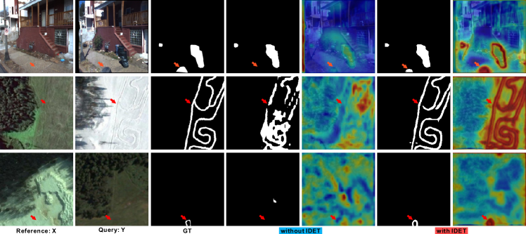
Figure 7: Three cases with/without IDET. The main advantages are highlighted via red arrows.

Differences to existing transformers. In this work, for the first attempt, explore the critical role of the feature difference quality to the CD (See Fig. 1). The intuitive idea of IDET is to extract difference information for the representations of input images (i.e., $\mathbf{R}_{\text{x}}$ and $\mathbf{R}_{\text{y}}$) and use them to guide the refinement of the feature difference $\mathbf{D}$. To this end, we propose a novel transformer-based module that is different from previous ones (See Fig. 4). First, the whole IDET is novel but not a naive combination of three transformers. The transformers $\tau_{\text{ref}}$ and $\tau_{\text{que}}$ are to extract difference-related information in corresponding features (i.e., $\mathbf{R}_{\text{x}}$ and $\mathbf{R}_{\text{y}}$), and we design an extra function $\text{diff}(\cdot)$ to further refine the semantic differences. Second, the transformer $\tau_{\text{diff}}$ is a dynamic transformer and basically different from existing ones while it allows borrowing the extra information (i.e., $\tilde{\mathbf{D}}$) to guide the updating of the input $\mathbf{D}$ dynamically (See Eq. (5)). Third, IDET allows the iterative optimization that benefits the detection accuracy significantly as demonstrated in Table IV. By replacing our IDET by a CNN model, we can see that F1 drops from 94.0 to 93.6. Also, $\tau_{\text{ref}}(\cdot)$, $\tau_{\text{que}}(\cdot)$ and $\tau_{\text{diff}}(\cdot)$ are replaced by a convolution layer to study each function in our IDET, which shows that $\tau_{\text{ref}}(\cdot)$ and $\tau_{\text{que}}(\cdot)$ benefit the CD performance more than $\tau_{\text{diff}}(\cdot)$.

TABLE IV: Ablation studies on multi scales and three transformers $\tau_{\text{ref}}(\cdot)$&$\tau_{\text{que}}(\cdot)$, $\tau_{\text{diff}}(\cdot)$ (3rd transformer). We use the convolution block (consists of four convolution layers with batch normalization and ReLU) to replace the IDET and get a variant (i.e., Multi-Scale-CNN-feat. diff. enhance.). We make this experiment on VL-CMU-CD. The bold is the best.

Methods	F1	OA	Iou
w/o feat. diff. enhance.	93.2	99.3	87.7
Multi-Scale-CNN-feat. diff. enhance.	93.6	99.3	88.0
Multi-Scale.IDET-feat. diff. enhance. (Ours)	94.0	99.4	88.7
Naive-Multi-Scale.IDET-feat. diff. enhance.	93.8	99.3	88.4
Single-Scale.IDET-feat. diff. enhance.	93.7	99.3	88.2
Multi-Scale.IDET w/o $\tau_{\text{diff}}(\cdot)$	0.935	0.993	0.879
Single-Scale.IDET w/o $\tau_{\text{diff}}(\cdot)$	0.933	0.993	0.875
Multi-Scale.IDET w/o $\tau_{\text{ref}}(\cdot)$&$\tau_{\text{que}}(\cdot)$	0.929	0.993	0.867
Single-Scale.IDET w/o $\tau_{\text{ref}}(\cdot)$&$\tau_{\text{que}}(\cdot)$	0.924	0.992	0.860

Visualization of the feature difference enhancement. We have visualized the importance of the feature difference enhancement in Fig. 1. Here, in Fig. 7, we further present three cases to compare the feature difference before and after enhancement ($5$th column vs. $7$th column) and detection results with/without IDET. Clearly, IDET enhances the desired changes in the feature difference map, leading to obvious advantages in final evaluations. Fig. 8 shows the detailed comparison of $\mathbf{M}$ under $\mathbf{D}$ and $\hat{\mathbf{D}}$ on six datasets, which can demonstrate that our IDET can improve the final results effectively.

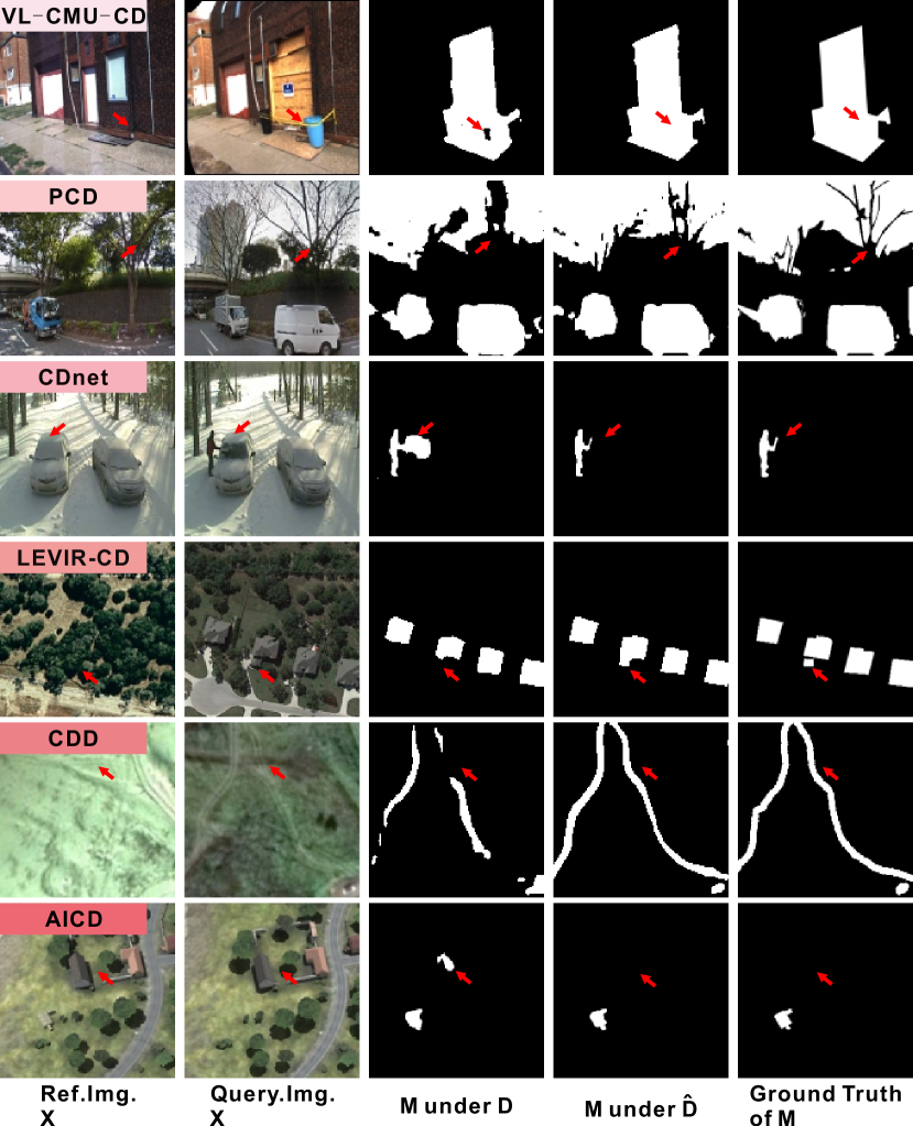
Figure 8: Comparison of M under D with M under $\hat{\textbf{D}}$ on six datasets.

TABLE V: Results of different $T$ in IDET. The bold is the best.

Dataset	CMU			PCD			CDnet			LEVIR			CDD			AICD
Iter	F1	OA	IoU	F1	OA	IoU	F1	OA	IoU	F1	OA	IoU	F1	OA	IoU	F1	OA	IoU
0	93.2	99.3	87.8	71.2	88.3	58.5	91.7	99.6	85.7	87.0	98.0	79.3	80.0	98.1	69.4	89.5	99.9	81.4
1	93.6	93.8	88.4	73.8	89.5	61.7	92.6	99.7	87.0	82.9	97.3	74.0	82.9	98.5	73.4	90.5	99.9	82.8
2	94.0	99.4	88.7	76.0	88.8	61.9	92.4	99.7	86.2	88.9	98.1	80.2	85.4	98.5	78.2	91.4	99.9	84.4
3	94.0	99.4	88.6	73.9	88.4	59.3	93.8	99.6	88.8	61.7	96.1	50.4	83.0	98.7	73.6	86.9	99.9	76.8
4	93.9	99.4	88.6	74.1	88.5	59.4	93.7	99.6	88.7	83.2	98.2	75.1	83.5	98.7	74.1	89.5	99.9	81.4
5	93.9	99.3	88.6	74.6	88.2	59.4	93.8	99.7	88.9	83.0	98.2	74.8	83.0	98.7	73.3	90.1	99.9	82.0

Effectiveness of multiple losses with Focal loss and Cross entropy loss. We add supervision on all predicted change maps of $\mathbf{M}^{0},\ldots,\mathbf{M}^{L}$ and $\mathbf{M}$ to train our model. To validate the effectiveness of using multiple supervision, we retrain our network only using single supervision on the final change map $\mathbf{M}$ with Cross entropy loss ($\mathcal{SS}+\mathcal{CE}$), multiple supervision with Focal loss ($\mathcal{MS}+\mathcal{F}$), and multiple supervision with Cross entropy loss ($\mathcal{MS}+\mathcal{CE}$). As shown in Table. VI, we find that ❶ using multiple supervisions ($\mathcal{MS}+\mathcal{CE}$) achieves consistently F1, OA and IoU improvements over using single supervision ($\mathcal{SS}+\mathcal{CE}$); ❷ using Cross entropy loss ($\mathcal{MS}+\mathcal{CE}$) is more suitable for CD than using Focal loss ($\mathcal{MS}+\mathcal{F}$).

TABLE VI: Results of our method with single supervision ($\mathcal{SS}$) on the final layer and multiple supervision ($\mathcal{MS}$), Focal loss ($\mathcal{F}$) and Cross entropy loss ($\mathcal{CE}$). The bold is the best.

Dataset	$\mathcal{SS}$+$\mathcal{C}$E			$\mathcal{MS}$+$\mathcal{F}$			$\mathcal{MS}$+$\mathcal{CE}$
	F1	OA	IoU	F1	OA	IoU	F1	OA	IoU
VL-CMU-CD	91.6	99.3	87.3	91.6	99.2	84.6	94.0	99.4	88.7
PCD	75.0	88.9	60.3	70.1	88.1	54.4	76.0	88.8	61.9
CDnet	92.4	99.6	86.1	89.9	99.5	81.6	92.4	99.7	86.2
LEVIR-CD	87.8	97.8	78.3	82.5	97.0	70.3	88.9	98.1	80.2
CDD	78.0	97.6	64.3	70.8	97.1	55.1	85.4	98.5	75.2
AICD	88.5	99.9	79.4	88.8	99.9	80.4	91.4	99.3	82.5

Iteration of IDET. We set different iteration numbers  ($T$) for IDET to study the influence of $T$. Table V shows the results of $T=0$, $T=1$ , …, and $T=5$ in IDET. Specifically, $T=0$ means that the difference convolutional features are directly used for CD without iterative difference-enhanced transformers. We can find that using our IDET can achieve better performances on each dataset than employing a convolution network, which demonstrates that IDET will improve the representational ability of different features. Specifically, our IDET achieves the best performances on most datasets when the $T=2$. Increasing $T$ does not further improve the CD performances on most of the datasets because larger $T$ makes the model become more complex, which needs longer training time. On CDnet, using $T=5$ achieves the best F1, OA, and IoU values than using $T=2$. A possible reason is that the training and testing image pairs on CDnet are captured from the same video, which results in a high correlation between the changes in the training and testing sets.

Results model complexity. In Table VII, we report the running time, GFLOPs and F1 of IDETs with $T\in\{0,1,2,3,4,5\}$ on VL-CMU-CD. We can find that the GFLOPS and running time become higher as $T$ increasing. The F1 values of our method increase from $T=0$ to $T=2$, dropping when continue increasing $T$. As the $T$ increasing, the running time and GELOPs are also increasing. Thus, $T=2$ is a good choice for the proposed method. To demonstrate the effectiveness of IDET, we replace IDET (T=2) with a CNN model containing four convolution blocks with convolution layer, batch normalization, and ReLU, which has much higher GFLOPS than IDET. As shown in Table VII, we find that the CNN-based method has a lower F1 value than IDET (T=2). Additionally, we also give the running time and GFLOPs of the compared methods in Table VII. CSCDnet has the longest running time with 214.8 ms. BIT has the shortest running time with 13.7 ms. Due to stacking four complex Transformer blocks, ChangeFormer has the highest GFLOPs of 316.9 among all the CD methods. IDET ($T=2$) has moderate GFLOPs and achieves the highest F1 value than other compared methods.

TABLE VII: Comparison on model efficiency. Running time (RT) and GFLOPs of IDET with different $T$ and comparison methods. We set a CNN model to replace the IDET and let it has even larger GFLOPS than the IDET (T=3). The input image size is $320\times 320\times 3$.

	RT(ms)	GFLOPs	F1
$T=0$	44.8	96.1	93.2
$T=1$	72.9	186.8	93.6
$T=2$	93.2	195.8	94.0
$T=3$	114.3	204.8	93.9
$T=4$	137.1	213.7	94.0
$T=5$	160.9	222.7	94.0
CNN w. similar model size	66.2	214.5	93.6
FCNCD	32.7	100.2	84.2
ADCDnet	41.3	217.4	93.5
CSCDnet	214.8	65.9	90.1
IFN	35.0	128.5	83.6
BIT	13.7	53.8	89.0
STAnet	66.2	20.1	82.9
ChangeFormer	100.2	316.9	88.3

Overfitting validation. We conduct cross-validation experiments across 3 datasets (i.e., VL-CMU-CD, CDnet, PCD) and compare with ADCDnet, CSCDnet, IFN, BIT in Fig. 9. ‘CMU2PCD’ means that we train detectors on VL-CMU-CD dataset and sample the testing images from the PCD dataset to evaluate. We can find that IDET has a higher generalization ability than all baseline methods.

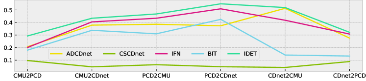
Figure 9: Cross validation of comparison methods (i.e. ADCDnet, CSCDnet, IFN, BIT) on VL-CMU-CD, PCD and CDnet datasets.

VI Conclusion

In this paper, we identify an important factor (i.e., the quality of feature difference) that affects the change detection accuracy significantly. To validate this, we built a basic feature difference-based change detection module and studied how the feature difference quality affects the final detection results. To fill this gap, we proposed a novel module (i.e., iterative difference-enhanced transformers (IDET)) to refine the feature difference. Moreover, to achieve better refinement, we proposed the multi-scale IDET and used it for the final change detection. We have conducted extensive experiments and ablation studies to compare the proposed method with the state-of-the-art methods as well as different variations on six large-scale datasets covering a wide range of application scenarios, image resolutions, and change ratios. Our method outperforms all baseline methods, which infers the importance of the feature difference quality.

References

- [1] N. Buch, S. A. Velastin, and J. Orwell, “A review of computer vision techniques for the analysis of urban traffic,” IEEE Transactions on intelligent transportation systems, vol. 12, no. 3, pp. 920–939, 2011.
- [2] D. Brunner, L. Bruzzone, and G. Lemoine, “Change detection for earthquake damage assessment in built-up areas using very high resolution optical and sar imagery,” in 2010 IEEE International Geoscience and Remote Sensing Symposium. IEEE, 2010, pp. 3210–3213.
- [3] M. Gong, J. Zhao, J. Liu, Q. Miao, and L. Jiao, “Change detection in synthetic aperture radar images based on deep neural networks,” IEEE transactions on neural networks and learning systems, vol. 27, no. 1, pp. 125–138, 2015.
- [4] S. H. Khan, X. He, F. Porikli, and M. Bennamoun, “Forest change detection in incomplete satellite images with deep neural networks,” IEEE Transactions on Geoscience and Remote Sensing, vol. 55, no. 9, pp. 5407–5423, 2017.
- [5] L. Mou, L. Bruzzone, and X. X. Zhu, “Learning spectral-spatial-temporal features via a recurrent convolutional neural network for change detection in multispectral imagery,” IEEE Transactions on Geoscience and Remote Sensing, vol. 57, no. 2, pp. 924–935, 2018.
- [6] K. Lin, S.-C. Chen, C.-S. Chen, D.-T. Lin, and Y.-P. Hung, “Abandoned object detection via temporal consistency modeling and back-tracing verification for visual surveillance,” IEEE Transactions on Information Forensics and Security, vol. 10, no. 7, pp. 1359–1370, 2015.
- [7] A. Albiol, L. Sanchis, A. Albiol, and J. M. Mossi, “Detection of parked vehicles using spatiotemporal maps,” IEEE Transactions on Intelligent Transportation Systems, vol. 12, no. 4, pp. 1277–1291, 2011.
- [8] H. Liu, S. Chen, and N. Kubota, “Intelligent video systems and analytics: A survey,” IEEE Transactions on Industrial Informatics, vol. 9, no. 3, pp. 1222–1233, 2013.
- [9] D. Liang, S. Kaneko, H. Sun, and B. Kang, “Adaptive local spatial modeling for online change detection under abrupt dynamic background,” in 2017 IEEE International Conference on Image Processing (ICIP). IEEE, 2017, pp. 2020–2024.
- [10] R. Huang, M. Zhou, Q. Zhao, and Y. Zou, “Change detection with absolute difference of multiscale deep features,” Neurocomputing, vol. 418, pp. 102–113, 2020.
- [11] L. Zhang, X. Hu, M. Zhang, Z. Shu, and H. Zhou, “Object-level change detection with a dual correlation attention-guided detector,” ISPRS Journal of Photogrammetry and Remote Sensing, vol. 177, pp. 147–160, 2021.
- [12] R. Huang, M. Zhou, Y. Xing, Y. Zou, and W. Fan, “Change detection with various combinations of fluid pyramid integration networks,” Neurocomputing, vol. 437, pp. 84–94, 2021.
- [13] J.-X. Zhao, Y. Cao, D.-P. Fan, M.-M. Cheng, X.-Y. Li, and L. Zhang, “Contrast prior and fluid pyramid integration for rgbd salient object detection,” in Proceedings of the IEEE/CVF Conference on Computer Vision and Pattern Recognition, 2019, pp. 3927–3936.
- [14] E. Guo, X. Fu, J. Zhu, M. Deng, Y. Liu, Q. Zhu, and H. Li, “Learning to measure change: Fully convolutional siamese metric networks for scene change detection,” arXiv preprint arXiv:1810.09111, 2018.
- [15] M. Zhang and W. Shi, “A feature difference convolutional neural network-based change detection method,” IEEE Transactions on Geoscience and Remote Sensing, vol. PP, no. 99, pp. 1–15, 2020.
- [16] J. Chen, Z. Yuan, J. Peng, L. Chen, H. Huang, J. Zhu, T. Lin, and H. Li, “Dasnet: Dual attentive fully convolutional siamese networks for change detection of high resolution satellite images,” IEEE Journal of Selected Topics in Applied Earth Observations and Remote Sensing, 2020.
- [17] Q. Wang, Z. Yuan, Q. Du, and X. Li, “Getnet: A general end-to-end 2-d cnn framework for hyperspectral image change detection,” IEEE Transactions on Geoscience and Remote Sensing, 2018.
- [18] R. Wang, F. Ding, J. W. Chen, B. Liu, and L. Jiao, “Sar image change detection method via a pyramid pooling convolutional neural network,” in IGARSS 2020 - 2020 IEEE International Geoscience and Remote Sensing Symposium, 2020.
- [19] X. Li and A. Yeh, “Principal component analysis of stacked multi-temporal images for the monitoring of rapid urban expansion in the pearl river delta,” International Journal of Remote Sensing, vol. 19, no. 8, pp. 1501–1518, 1998.
- [20] W. A. Malila, “Change vector analysis: an approach for detecting forest changes with landsat,” in LARS symposia, 1980, p. 385.
- [21] A. Vaswani, N. Shazeer, N. Parmar, J. Uszkoreit, L. Jones, A. N. Gomez, Ł. Kaiser, and I. Polosukhin, “Attention is all you need,” in Advances in neural information processing systems, 2017, pp. 5998–6008.
- [22] A. Dosovitskiy, L. Beyer, A. Kolesnikov, D. Weissenborn, X. Zhai, T. Unterthiner, M. Dehghani, M. Minderer, G. Heigold, S. Gelly, et al., “An image is worth 16x16 words: Transformers for image recognition at scale,” arXiv preprint arXiv:2010.11929, 2020.
- [23] G. Sun, Y. Liu, T. Probst, D. P. Paudel, N. Popovic, and L. Van Gool, “Boosting crowd counting with transformers,” arXiv preprint arXiv:2105.10926, 2021.
- [24] Y. Li, K. Zhang, J. Cao, R. Timofte, and L. Van Gool, “Localvit: Bringing locality to vision transformers,” arXiv preprint arXiv:2104.05707, 2021.
- [25] N. Carion, F. Massa, G. Synnaeve, N. Usunier, A. Kirillov, and S. Zagoruyko, “End-to-end object detection with transformers,” in European Conference on Computer Vision. Springer, 2020, pp. 213–229.
- [26] H. Touvron, M. Cord, M. Douze, F. Massa, A. Sablayrolles, and H. Jégou, “Training data-efficient image transformers & distillation through attention,” in International Conference on Machine Learning. PMLR, 2021, pp. 10 347–10 357.
- [27] X. Zhu, W. Su, L. Lu, B. Li, X. Wang, and J. Dai, “Deformable detr: Deformable transformers for end-to-end object detection,” arXiv preprint arXiv:2010.04159, 2020.
- [28] S. Zheng, J. Lu, H. Zhao, X. Zhu, Z. Luo, Y. Wang, Y. Fu, J. Feng, T. Xiang, P. H. Torr, et al., “Rethinking semantic segmentation from a sequence-to-sequence perspective with transformers,” in Proceedings of the IEEE/CVF Conference on Computer Vision and Pattern Recognition, 2021, pp. 6881–6890.
- [29] Z. Liu, Y. Lin, Y. Cao, H. Hu, Y. Wei, Z. Zhang, S. Lin, and B. Guo, “Swin transformer: Hierarchical vision transformer using shifted windows,” arXiv preprint arXiv:2103.14030, 2021.
- [30] X. Dong, J. Bao, D. Chen, W. Zhang, N. Yu, L. Yuan, D. Chen, and B. Guo, “Cswin transformer: A general vision transformer backbone with cross-shaped windows,” arXiv preprint arXiv:2107.00652, 2021.
- [31] E. Xie, W. Wang, Z. Yu, A. Anandkumar, J. M. Alvarez, and P. Luo, “Segformer: Simple and efficient design for semantic segmentation with transformers,” arXiv preprint arXiv:2105.15203, 2021.
- [32] D. Liang, X. Chen, W. Xu, Y. Zhou, and X. Bai, “Transcrowd: Weakly-supervised crowd counting with transformer,” arXiv preprint arXiv:2104.09116, 2021.
- [33] Z. Q. Hao Chen and Z. Shi, “Remote sensing image change detection with transformers,” IEEE Transactions on Geoscience and Remote Sensing, pp. 1–14, 2021.
- [34] W. G. C. Bandara and V. M. Patel, “A transformer-based siamese network for change detection,” arXiv preprint arXiv:2201.01293, 2022.
- [35] C. Zhang, P. Yue, D. Tapete, L. Jiang, B. Shangguan, L. Huang, and G. Liu, “A deeply supervised image fusion network for change detection in high resolution bi-temporal remote sensing images,” ISPRS Journal of Photogrammetry and Remote Sensing, vol. 166, pp. 183–200, 2020.
- [36] P. F. Alcantarilla, S. Stent, G. Ros, R. Arroyo, and R. Gherardi, “Street-view change detection with deconvolutional networks,” Autonomous Robots, vol. 42, no. 7, pp. 1301–1322, 2018.
- [37] O. Ronneberger, P. Fischer, and T. Brox, “U-net: Convolutional networks for biomedical image segmentation,” in International Conference on Medical image computing and computer-assisted intervention. Springer, 2015, pp. 234–241.
- [38] A. Paszke, S. Gross, S. Chintala, G. Chanan, E. Yang, Z. DeVito, Z. Lin, A. Desmaison, L. Antiga, and A. Lerer, “Automatic differentiation in pytorch,” 2017.
- [39] H. Chen and Z. Shi, “A spatial-temporal attention-based method and a new dataset for remote sensing image change detection,” Remote Sensing, vol. 12, no. 10, p. 1662, 2020.
- [40] K. Sakurada and T. Okatani, “Change detection from a street image pair using cnn features and superpixel segmentation,” in Proceedings of the British Machine Vision Conference (BMVC). BMVA Press, 2015, pp. 61.1–61.12.
- [41] N. Goyette, P.-M. Jodoin, F. Porikli, J. Konrad, and P. Ishwar, “Changedetection. net: A new change detection benchmark dataset,” in 2012 IEEE computer society conference on computer vision and pattern recognition workshops. IEEE, 2012, pp. 1–8.
- [42] J. Long, E. Shelhamer, and T. Darrell, “Fully convolutional networks for semantic segmentation,” in Proceedings of the IEEE conference on computer vision and pattern recognition, 2015, pp. 3431–3440.
- [43] K. Sakurada, M. Shibuya, and W. Wang, “Weakly supervised silhouette-based semantic scene change detection,” in 2020 IEEE International conference on robotics and automation (ICRA). IEEE, 2020, pp. 6861–6867.
- [44] Shunping, Ji, Shiqing, Wei, Meng, and Lu, “Fully convolutional networks for multisource building extraction from an open aerial and satellite imagery data set,” IEEE Transactions on Geoscience and Remote Sensing, vol. 57, no. 1, pp. 574–586, 2019.
- [45] N. Bourdis, D. Marraud, and H. Sahbi, “Constrained optical flow for aerial image change detection,” in 2011 IEEE International Geoscience and Remote Sensing Symposium. IEEE, 2011, pp. 4176–4179.