Assaying Out-Of-Distribution
Generalization in Transfer Learning

Abstract

Since out-of-distribution generalization is a generally ill-posed problem, various proxy targets (e.g., calibration, adversarial robustness, algorithmic corruptions, invariance across shifts) were studied across different research programs resulting in different recommendations. While sharing the same aspirational goal, these approaches have never been tested under the same experimental conditions on real data. In this paper, we take a unified view of previous work, highlighting message discrepancies that we address empirically, and providing recommendations on how to measure the robustness of a model and how to improve it. To this end, we collect $172$ publicly available dataset pairs for training and out-of-distribution evaluation of accuracy, calibration error, adversarial attacks, environment invariance, and synthetic corruptions. We fine-tune over $31\mathrm{k}$ networks, from nine different architectures in the many- and few-shot setting. Our findings confirm that in- and out-of-distribution accuracies tend to increase jointly, but show that their relation is largely dataset-dependent, and in general more nuanced and more complex than posited by previous, smaller scale studies¹.

1 Introduction

With deep learning enabling a variety of downstream applications [41, 53, 52, 29], failures of robustness leading to systematic [11, 33, 40] and catastrophic deployment errors [83, 25, 12] have become increasingly relevant. From early work on studying distribution shifts [e.g., 14, 15] and the classical “cow on the beach” example (e.g., in [13]), several works have highlighted sometimes spectacular failures of machine learning when the test distribution differs from training [100, 10, 98, 43, 48, 68, 88, 12, 94]. This has motivated the study of different types of distribution shifts, ultimately branching the field into several sub-communities that, while sharing the same underlying objective, rely on different evaluation protocols and provide different recommendations to practitioners.

(1) The studies [43, 68, 48, 88, 7, 10, 31] focused on algorithmically corrupting upstream pre-training datasets [90] to test generalization. Perhaps unsurprisingly, the choice of augmentations can significantly alter this notion of robustness [92, 22, 45, 44, 89]. (2) As synthetic corruptions need not transfer to real world distribution shifts [45], new realistic datasets were collected to test upstream robustness [10, 86, 97, 45, 110, 46]. Here, scale has been identified as a reliable ingredient [28, 69, 116, 86, 121], despite other works [118] arguing that extensive upstream pre-training can harm downstream robustness. (3) Exhaustive comparisons attempted to disentangle intrinsic architectural robustness from specific training schedules [16, 72, 9, 67, 78, 17], addressing underspecification [24] with inductive biases. Orthogonally, several (less scalable) works advocated for leveraging the compositional (perhaps causal [93]) structure in the underlying data-generative process to introduce suitable inductive biases [76, 37, 64, 63, 27, 81, 36]. (4) Simultaneously, Bayesian approaches for uncertainty predictions have been proposed to improve model calibration [73, 2, 65, 111, 59, 112, 123, 35] and robustness on new distributions [74, 113, 109]. Recent work, however, found that larger models were natively better calibrated [70]. (5) The adversarial training community developed an entire literature on different worst case local perturbations of training data [100, 66], with $5000$+ papers written to date [1] and a never ending cycle of new defenses and attacks [6, 75, 84, 85, 21]. (6) Other niche approaches investigated carefully designed test sets [91, 57, 38] and training protocols that promote invariance across several distributions [5, 91, 19, 77, 54]. Despite this progress, empirical risk minimization (ERM) remains a strong contender [38]. Overall, the significant community effort towards more robust machine learning models have resulted in diverse proxy evaluation targets yielding different practical recommendations.

At the same time, the workflow of successful applications developed in the opposite direction  [52, 29, 80, 82, 87]. Instead of collecting large application-specific datasets, one trains generalist backbones on the greatest possible amount of data and then transfers the model using available domain-specific examples. Besides the test data likely being “on manifold”, one is almost certainly guaranteed that there will be some sort of distribution shift at test time as the size of the fine-tuning dataset decreases.

Focusing on classification of visual data, we evaluate the different key metrics from these communities in a unified manner and under the same experimental conditions to investigate the gaps in common practices. We restrict ourselves to the realistic situation where we have an ImageNet pre-trained model available and a new target distribution as downstream task. After the model has been fine-tuned, the test data may be OOD. From $36$ existing datasets, we extract $172$ in-distribution (ID) and out-of-distribution (OOD) dataset pairs, fine-tuning and evaluating over $31\mathrm{k}$ models to gain a broader insight in the sometimes contradicting statements on OOD robustness in previous research. We organize our study around two key questions: (1) What are good proxy measures of OOD robustness when having access to a single dataset? (2) How do architecture choices and fine-tuning strategies affect robustness? We plan to publish the code with the camera-ready version of the paper.

Our key contributions are (1) We conduct a large systematic study of OOD robustness, evaluating the effect of architecture type, augmentation, fine-tuning strategies and few-shot learning. We investigate the interplay of robustness to corruptions, adversarial robustness, robustness to natural distribution shifts, calibration and other robustness metrics in a unified setting and under the same experimental conditions. (2) We find that out-of-distribution generalization has many facets. Insights of previous papers—sometimes presented as general conclusions— hold only on a subset of the tasks/datasets included in our study and hence actually only reflect a special case. (3) In general, in-distribution classification error (accuracy) is the best predictor of OOD accuracy, but other secondary metrics can provide additional insights. (4) With these results, we revisit previous studies and recommendations, reinterpreting their conclusions, resolving some contradictions, and suggesting critical areas for further research.

2 Experimental setup

We follow the modern workflow of applications of computer vision to (long-tail) downstream tasks from existing pre-trained backbones. The model is transferred using a set of (potentially few) examples from a new distribution. At test time, we assume that the classes remain the same (closed-world setting), but that the distribution may otherwise change. We specifically focus on the effect of distribution shifts after a model has been transferred to a new distribution (i.e., the downstream implications) and discuss the empirical differences and similarities compared to results concerning upstream OOD robustness that were discussed in previous studies [10, 86, 97, 110, 46, 28, 45].

Experimental protocol and datasets: We evaluate nine state-of-the-art deep learning models with publicly available pre-trained weights for ImageNet1k / ILSVRC2012 [90]. We consider $36$ datasets grouped into ten different tasks sharing the same labels. Datasets of the same task represent a set of natural distribution shifts. For each task, we take a single training dataset to fine-tune the model and report evaluation metrics on both its ID test set and all the other OOD test sets. We extract $172$ (ID, OOD) dataset pairs from the different domains of the ten tasks: DomainNet [79], PACS [56], SVIRO [26], Terra Incognita [13] as well as the Caltech101 [34], VLCS [104], Sun09 [18], VOC2007 [32] and the Wilds datasets [51] (from which we extract two tasks). In our experimental protocol we do not make any assumptions on the particular shift type and the considered tasks reflect multiple shift types (e.g., presumably a strong covariate shift in DomainNet and a partial label shift in Camelyon17 of the Wilds benchmark). See Appendix E for a detailed overview. Models are fine-tuned on a single GPU using Adam [50] with a batch-size of $64$ and a constant learning rate.

Evaluation on ID, OOD and corrupted data: Some tasks, such as DomainNet, PACS and SVIRO come with different datasets/domains. For those, we report for each dataset the ID (test) performance and the OOD (test) performances on the other datasets in the task. For the datasets from the WILDS benchmark, we use the provided ID test and OOD test splits. If a task consists of multiple OOD data we compute the metrics additionally on held-out OOD data. To do so, for each (ID, OOD) dataset pair, we average the performance on the remaining OOD datasets. This approach is sometimes called multi-domain evaluation [e.g., 109]. Alongside the provided OOD datasets, we evaluate the models on the corrupted ID test set. We apply $17$ types of corruptions from [43] each with $5$ severity levels. The corrupted version of the datasets can be viewed as a synthetic distribution shift and we investigate how informative they are of natural distribution shifts.

Models: To ensure that our results are relevant for researchers and practitioners alike, we consider both widely deployed and recent top-performing methods: Resnet50d [42], DenseNet [47], EfficientNetV2 [101], gMLP [58], MLP-Mixer [103], ResMLP [105], Vision Transformers [29], Deit [106], Swin Transformer [60]. We list the exact model names in Table S4. Our choice of models covers convolutional networks, transformer variants and mixers. Weights for the pre-trained models were taken from the PyTorch Image Models repository [114].

Model hyperparameters and augmentation strategies: For each model we consider the learning rate and the number of fine-tuning epochs. We first ran a large sweep over these two hyperparameters on a subset of the experiments and used it to pre-select a set of four parameter combinations that included the best performing models for each architecture. Additionally, we study three different augmentation strategies: standard ImageNet augmentation (i.e., no additional augmentation), RandAugment [23] and AugMix [44]. More details can be found in Appendix H.

Fine-tuning strategy and few-shot training: We investigate fine-tuning the full architecture and fine-tuning only the head. Additionally, we consider three training paradigms: training on the full downstream dataset, and two few-shot settings: “few-shot-$100$” (a subset with $100$ examples per class, if available) and “few-shot-$10$” (with $10$ examples per class). In the few-shot settings, the images are randomly selected, and classes that have fewer images as the cap of $10$ or $100$, respectively, are not over-sampled.

Metrics: We pick some of the most popular metrics that are used to measure progress towards robust machine learning. We report six different metrics: classification error, negative log-likelihood (NLL), demographic disparity [30, 61] on inferred groups [19] as a measure of invariance, the expected calibration error (ECE) [39], and adversarial classification error for two different $\ell_{2}$-attack sizes. The metrics are, where applicable, evaluated on ID, OOD, and corrupted test sets, (except adversarial error, which we did not evaluate on the corrupted test sets). See Appendix G for more details.

3 Additional related work

As much of the related work was already mentioned in the introduction we highlight two main areas of closely related works: one regarding benchmarks for generalization to new distributions and one on the interplay between different evaluation metrics.

Benchmarking robustness to OOD. Closely to our setting, [119] benchmarked models in a few-shot learning setting but did not analyze the robustness of the fine-tuned models. In follow up work, [28] related the results of [119] to upstream robustness but did not consider downstream distribution shifts. [38] analyzed a variety of domain generalization algorithm and found that none of them could beat a strong ERM baseline. While several of our datasets overlap with theirs, we consider the transfer learning setting as opposed to domain generalization. Their insights may be in part explained by the fact that the regularization is either orthogonal to OOD accuracy or simply harms accuracy overall as in [124]. [115, 94] proposed a model for analyzing different fine-grained distribution shifts. Their work is limited to few datasets and model types and only cover accuracy evaluations. [49] studied the effect of the pre-training strategy on domain generalization and [107] studied extensions to large pre-trained models for improved reliability, whereas our work analyzes fine-tuning protocols and the robustness on downstream tasks. [45] found that larger models and better augmentation techniques improve robustness but did not consider different model types, augmentation techniques or evaluation metrics. Our work studies robustness in a larger scope than previous work, which focused on certain dimensions of our empirical investigations. None of the previous work studied the interplay of different robustness metrics.

Studying the interplay of robustness metrics. There has been only limited work on analyzing informativeness of robustness metrics on OOD generalization. [102] analyzed distribution shifts of ImageNet and found that corruption metrics do not imply robustness to natural shift. Recently, [69], based on previous studies by [102, 95, 10, 96], observed a clear linear relationship between ID accuracy and OOD accuracy and hypothesized that this could be a general pattern in contradiction to [24]. [8] extended this line of work to agreement between networks and [4] found that large pre-trained models are above the linear trend in early stages of fine-tuning. However, our extended set of experiments show that a clear linear trend is only visible on some (ID, OOD) dataset pairings. [108] empirically investigated different generalization measures and found that measures relating to the Fisher information perform best.

4 A broad look at out-of-distribution generalization

In the following we explore the facets of out-of-distribution generalization, highlighting discrepancies to prior work and discuss their implications.

4.1 The main latent factors that explain the empirical results

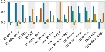
Figure 1: Factor loadings (contributions) of different metrics based on a factor analysis with 4 orthogonal factors (color-coded), highlighting similarities between the metrics. The factor Blue: captures classification error, adversarial error, log-likelihood, and their corrupted variants. Green: only in OOD metrics. Yellow: expected calibration error. Red: demographic disparity.

To get a first overview of the relations between the different metrics and their generalization properties, we perform a factor analysis to discover the main orthogonal latent factors that explain the variance in the metrics evaluated on each ID dataset, its corrupted variant, and the metrics averaged over all compatible OOD datasets for each fine-tuned model. For details, see Appendix B.

Based on the scree plot in Appendix B, we retain four factors. Their contributions (loadings) to each metric are shown in Fig. 1. Interestingly, each factor has a clear interpretation. Factor 1 (blue) is very well aligned with ID classification error, log-likelihood and adversarial attacks. Factor 2 (green) captures OOD-specific variance, since it is particularly pronounced in almost every out-of-distribution metric, and only there. Factor 3 (orange) relates mainly to the expected calibration error and factor 4 (red) to demographic disparity. The dominant presence of factor 1 (blue) in all classification error and log-likelihood metrics ID and OOD suggests that ID classification error can be a reasonably good predictor of OOD classification error, which we further discuss in Section 4.3. However, the presence of an OOD-specific factor also suggests that ID versus OOD accuracy (classification error) cannot always lie “on a line” [69]—we investigate this further in Section 4.2. Another noteworthy point is that the corrupted metrics and adversarial classification errors have almost no OOD component and are generally very close to the corresponding ID metric. Similarly, the loadings of the corrupted metrics are much closer to those of the ID metrics than to OOD metrics. This suggests that the performance on artificially corrupted data may not predict the OOD performance significantly better than the bare ID metrics. We further discuss this in Section 4.3.2. Finally, the fact that demographic disparity and expected calibration error are each mainly captured by their own, specific factor suggests that, maybe surprisingly, those metrics are largely independent of the networks’ classification error. Further details are discussed in Section 4.3.2.

4.2 The many facets of out-of-distribution generalization

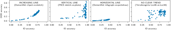
Figure 2: Typical scatter plot patterns observed in our data (see Appendix D for all plots). Increasing line: ID and OOD accuracy show a clear functional dependency. In contrast to previous claims this is not the typical setting (only observed on a subset of datasets). Vertical line: the same ID peformance leads to different OOD behavior (underspecification setting). Horizontal line close to zero accuracy: no transfer of information from the ID to the OOD dataset. No clear trend: random associations between ID and OOD accuracy (i.e., zero correlation).

Prior publications [69, 102, 28] observed that OOD accuracy strongly linearly correlates with ID accuracy, or, in other words, that ID vs OOD accuracy nearly lie “on a line”. In contrast, we find that this is not a general trend when tested on more tasks. Fig. 2 shows the four typical settings we observe. For some (ID, OOD) dataset pairs we observe a clear functional dependency as claimed by [69, 102] (increasing line). For other dataset pairs we observe a clear underspecification problem [24]: very similar ID performances (in most cases close to $1$) lead to different OOD performances (vertical line). In this setting, ID accuracy is not a sufficient model selection criterion for obtaining robust models. In some settings, the models do not transfer information from the ID to the OOD data at all and, despite having different ID performance, all models have very poor OOD performance. Finally, we observe a fourth setting, where OOD accuracy is hardly correlated to ID accuracy. Interestingly, we never see a decreasing trend, i.e., improved ID performance never systematically results into lower OOD performance. Hence, despite the many shapes of ID and OOD dependency, it is still a good strategy to maximize the ID accuracy in order to maximize the OOD accuracy.

Results can significantly change for different shift types. We highlighted how much ID to OOD generalization can change on different tasks/datasets. This is further confirmed by the task-specific correlation matrices in Sections A.3 and A.4, which, more generally, show that there can be significant differences in various metrics between different tasks or shift types. For example, comparing the terra-incognita and wilds-fmow specific correlation matrices, we see that for terra-incognita calibration and demographic disparity have a strong positive correlation with OOD accuracy, whereas for wilds-fmow the correlation is strongly negative. Similarly, multi-domain calibration as proposed by [109] only improves OOD robustness on some tasks, but has a negative effect on others (details in Section 4.3). Section A.4 shows that focusing on different shift types can also lead to contradicting findings. For instance, for models that were trained on artificial data (such as sketches, clipart, simulated environments) and evaluated on real OOD data, corruption metrics are more predictive of OOD robustness than for models that were trained on real data and tested on artificial OOD data. Additionally, we discuss in Section E.1 the dependence of the results on the task difficulty.

4.3 What are good proxies to measuring robustness to distribution shifts?

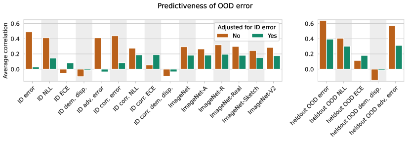
Figure 3: left: What is a good proxy for classification error under natural distribution shifts? We measure how well several popular robustness metrics on in-distribution (ID) data predict classification error on out-of-distribution (OOD) datasets. Red bars: The predictiveness score is computed based on Spearman’s rank correlation coefficient between the robustness metric and OOD classification error. We find that, among all considered metrics, ID classification error is the strongest predictor of OOD robustness. What is the additional information content of the robustness metrics adjusted for ID classification error? Green bars: We compute the adjusted predictiveness scores as outlined in Section 4.3. When adjusted for ID classification error, all secondary metrics only provide limited information. right: How predictive are the metrics on additional held-out OOD data? Evaluating accuracy on held-out OOD data (multi-domain evaluation) is the strongest predictor of OOD accuracy and provides significant additional information to ID accuracy (see adjusted scores).

Can we predict the robustness of a model by using a proxy measure? In other words, how predictive is a certain metric $A$ (e.g., ID expected calibration error) of another metric $B$ (e.g., OOD classification error)? To this end we compute the averaged correlation matrix which reports the rank correlation of all metrics, averaged over all tasks. The matrix and details on the method are deferred to Appendix A. We already saw –and the matrix confirms– that accuracy is a strong predictor of OOD accuracy. This raises the question if other metrics add any additional information on OOD accuracy which is not already provided by ID accuracy. To test this, we compute adjusted predictiveness scores as follows. For each dataset pair, we fit a linear regression to predict OOD accuracy from ID accuracy. We then report the averaged rank correlation coefficient between the obtained residuals and each metric. This measure is similar to the effective robustness proposed in [69]. Results are shown in Fig. 3 and discussed in the upcoming subsections.

4.3.1 Overall classification error is the best general predictor of OOD robustness

Fig. S1, derived from the full averaged correlation matrix in Appendix A, shows that among all considered metrics, ID classification error is the strongest predictor of OOD classification error. This finding is in contrast to works that hypothesized that evaluating the classification error on corrupted data (e.g., ImageNet-C [43]) or on adversarial perturbed data [117] provides additional information on how models perform under natural distribution shifts. Although these metrics show a high correlation with OOD classification error, we do not find that they add significant information when adjusting for ID classification error. However, when having access to additional OOD datasets, the classification error on the held-out OOD datasets is even more powerful predictor of the robustness of the OOD dataset of interest, see Fig. 3 (right). We find that this is the most reliable model selection procedure of all considered metrics.

Our findings imply that if practitioners want to make the model more robust on OOD data, the main focus should be to improve the ID classification error. This is in accordance with previous work that found that models with high ID classification error tend to be more robust [69, 28]. We speculate that the risk of “overfitting” large pre-trained models to the downstream test set is minimal, and it seems to be not a good strategy to, e.g., reduce the capacity of the model in the hope of better OOD generalization [118]. Finally, we recommend that architectural innovations and training techniques can leverage scale but that robustness comparisons should always be adjusted for classification error.

4.3.2 What can we learn from other metrics beyond accuracy?

The first interesting result is that calibration on ID data is not predictive of OOD robustness or OOD log-likelihood (see Fig. S1 in the appendix). Restricted to the ID regime, however, we observe a correlation between ID calibration and ID classification error, which is in accordance with [70]. This difference is explained by the fact that ID calibration is not predictive of OOD calibration without an OOD held-out set (see Section 4.4). In contrast to the observations in [109], we see that a model that is well-calibrated on multiple domains (held-out OOD data) may not always have lower OOD classification error (e.g., negative correlation for domain-net but positive on office-home, see Section A.3). Interestingly, invariance measured with environment inference [19] and demographic disparity [61] is not predictive of OOD robustness but seems to be a good proxy for calibration of OOD data (see Fig. S1) which is consistent with our observations on multi-domain calibration and may be useful for OOD detection.

ID log-likelihood and adversarial accuracy are both weak predictors of OOD robustness compared to ID accuracy, and when adjusted for ID accuracy they only add marginal to no information. Since the correlation between ID adversarial classification error and OOD classification error is fully explained by ID accuracy (see Fig. 3, left) suggests that adversarial distribution shifts do not characterize well natural distribution shifts.

Synthetic corruptions We apply the synthetic corruptions proposed by [43] to all datasets. First, we find that classification error and log-likelihood evaluated on the corrupted data are strongly correlated to OOD classification error (see Fig. 3, left). However, we find that the information provided by the corrupted metrics is significantly reduced when adjusted for ID accuracy. With the partial exception of corrupted calibration being more informative of OOD calibration than ID calibration (see Section 4.4). In summary, evaluation on corrupted data does not seem to bring the same benefits as using real held-out OOD data (see Fig. 3, right). Interestingly, we find that adversarial classification error is highly correlated to the classification error under synthetic corruptions (see Fig. S1). Therefore, if the practitioner cares about shifts defined by artificial corruptions, studying the adversarial robustness on ID data will be informative.

Robustness to upstream dataset shifts In our study all models are pre-trained on ImageNet (upstream dataset) and then fine-tuned on downstream data. In this section, we explore if upstream robustness propagates downstream. First, we notice in Fig. 3 (left) that the original performance on ImageNet is linked to OOD classification error in accordance to previous studies [28]. When we adjust for ID classification error, the clean ImageNet performance is among the strongest predictors for OOD classification error. Second, we find that robustness on ImageNet shifts does not give much additional information to the downstream robustness compared to clean performance. The performance on ImageNet shifts is almost perfectly correlated with the ID performance (in this setting accuracy is perfectly “on the line”, c.f. Section 4.2), but this relationship does not translate to our diverse set of downstream shifts.

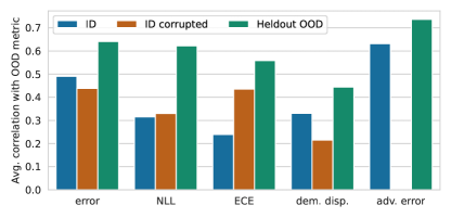
Figure 4: For each source metric on the x-axis we display the averaged correlation with the same metric evaluated on OOD data (target). The different colors indicate on which data domain the source metric was evaluated; either on ID, ID corrupted, or held-OOD data. Note that in our study we do not evaluate adversarial classification error on corrupted data.

4.4 On the transfer of metrics from ID to OOD data

The main focus of Section 4.3 was to analyze how informative the different metrics are of OOD classification error. In a more general setting, we now explore how well a metric evaluated on ID data predicts their score on OOD data. Fig. 4 shows the averaged correlation coefficient of each metric—evaluated either on ID, corrupted or held-out data—with the same metric evaluated on OOD data. First, we find that all ID metrics transfer moderately well to OOD data (blue bars). For adversarial attacks the transfer is highest. This suggests that the models respond similarly to adversarial attacks on ID data and on OOD data. On the other hand, ID calibration transfers worst among all metrics, i.e., a model that is well calibrated on ID data, is not necessarily well calibrated on OOD data. This points to an important problem, since in many production systems models are only calibrated on ID data. Second, we observe that the evaluation on corrupted data does not add significant information to the evaluation on ID data (blue vs. red bars) for most metrics. Interestingly, we observe one exception; for calibration the evaluation on corruptions is significantly more informative. Third, when having access to additional held-out data, the evaluation on this data is the strongest predictor for the OOD behavior for all metrics (green bars).

5 The effect of the training strategy on out-of-distribution robustness

We now investigate the influence of the training strategy and model architecture on OOD robustness for practitioners. Although we will observe clear trends, they should be taken with care, since each model was pre-trained with its own training procedure (with different optimizers, learning rate schedules, augmentations, sometimes even datasets, etc.), which is likely to confound downstream results even after using a unified fine-tuning procedure. This is a general problem since different architectures usually require a specific pre-training procedure. Most practitioners usually undergo the same pipeline, starting from a network with publicly available pre-trained weights.

5.1 The effect of augmentations, fine-tuning strategy and few-shot learning

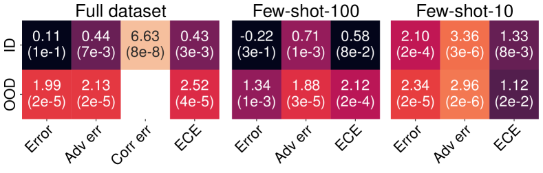
Figure 5: Performance gap (difference) between models trained with and without augmentations together with a p-value in parenthesis to assess its significance. Black fields indicate a p-value above the 0.05 significance threshold (i.e., non-significant); the other values are significant. Overall, augmentations help increasing the model’s accuracy and its robustness to all kinds of distribution shifts (artificial and adversarial corruptions, OOD generalization), more so when data is scarce (few-shot settings).

Model	ID Error	OOD Error	OOD-ID Gap
Deit	0.101 $\pm$ 0.005	0.364 $\pm$ 0.008	0.263 $\pm$ 0.006
Swin	0.111 $\pm$ 0.005	0.371 $\pm$ 0.008	0.260 $\pm$ 0.006
ViT-B	0.124 $\pm$ 0.005	0.384 $\pm$ 0.008	0.259 $\pm$ 0.006
ResNet50	0.124 $\pm$ 0.005	0.406 $\pm$ 0.008	0.283 $\pm$ 0.006
EfficientNet2	0.129 $\pm$ 0.005	0.407 $\pm$ 0.008	0.277 $\pm$ 0.006
GMLP	0.140 $\pm$ 0.006	0.413 $\pm$ 0.008	0.273 $\pm$ 0.006
ResMLP	0.134 $\pm$ 0.005	0.413 $\pm$ 0.008	0.279 $\pm$ 0.006
Mixer	0.142 $\pm$ 0.006	0.425 $\pm$ 0.008	0.282 $\pm$ 0.006
DenseNet169	0.145 $\pm$ 0.005	0.443 $\pm$ 0.008	0.298 $\pm$ 0.006

Table 2: Average classification error of model architectures with the standard error of this average in grey. To simulate a typical transfer learning workflow, we selected the best performing augmentations based on ID validation data for each fine tuning domain.

To evaluate the effect of augmentations during fine-tuning, we average the performance of networks trained with RandAugment [23] and AugMix [44] and compare it to fine-tuning without augmentations. Fig. 5 shows the performance gap between models trained with and without augmentations together with the p-value of a one-sided Wilcoxon signed-rank test that assesses whether the model trained without augmentations is better than the other one. Overall, augmentations appear to increase accuracy across all corruption types (natural, corrupted and adversarial data), particularly on OOD data. This suggests that augmentations not only improve accuracy in distribution, but also increase the model’s robustness under certain shifts. The effect is more pronounced when data is scarce (few-shot setting), although exceptions exist (accuracy in “few-shot-$100$”). We discuss additional results in Section C.2.

Previous studies have shown that the fine-tuning strategy significantly affects the robustness [115, 3, 55]. In our study we investigate two popular fine-tuning methods: (1) fine-tuning the full architecture and (2) fine-tuning the head only, while keeping the rest of the architecture frozen. We discuss the results in Section C.1 and find that fine-tuning the full architecture is better for most of the considered tasks when having access to the full datasets. However, in the low data regime (few-shot-10 setting), fine-tuning the head only is beneficial on 40% of the tasks.

5.2 The effect of the model architecture

With many pre-trained backbones available in libraries like [114] that often achieve very similar results on ImageNet, it is not obvious whether the architecture choice matters. Table 2 shows the average ID and OOD classification errors of each model. Interestingly, we observe that while the Vision Transformer ViT-B was trained on more data it performs worse than Swin- and Deit-Transformers both on ID and OOD data (both approx. $3\,\%$ higher error than Deit). This indicates that the extensions made to vision transformers improve generalization performance in the transfer learning and fine-tuning scenario, while additionally requiring less data. Further, we notice that the model with lowest average OOD classification error, does not show the lowest performance gap, i.e., the performance on ID data and OOD data are not necessarily more closely aligned when performance on ID and OOD accuracy increases.

6 Conclusions

In this paper, we thoroughly investigated out-of-distribution generalization and the interplay of several secondary metrics in the transfer learning setting. We focused on understanding sometimes contradicting empirical evidence from previous studies and on reconciling the results with anecdotal evidence from common practice in computer vision. We fine-tuned and evaluated over $31\mathrm{k}$ models across several popular architectures on $172$ (ID, OOD)-dataset pairs and found the following. (1) The risk of overfitting on the transfer distribution appears small: models that perform better in distribution tend to perform better OOD. All other proxy metrics convey only limited information on OOD performance after adjusting for ID accuracy. (2) Out-of-distribution generalization is a multi-faceted concept that cannot be reduced to a problem of “underspecification” [24] or to simple linear relations between ID and OOD accuracies [69]. However, we did not observe any trade-off between accuracy and robustness, as is commonly assumed in the domain generalization literature [5, 91, 19, 77, 54]. While such trade-offs may exist, we posit that they may not be very common in non-adversarially chosen test sets. (3) While calibration appears to transfer poorly to new distributions, adversarial examples and synthetic corruptions transfer well to OOD data but seem ill-suited to mimic natural distribution shifts. (4) Held-out OOD validation sets can be good proxies for OOD generalization. As such, they should be a key focus of any practitioner who worries about distribution shifts at test time.

In light of these results, we suggest three critical areas for further research. (1) Creating synthetic interventional distributions is an appealing alternative to hand-crafted augmentations and corruptions to both evaluate and improve robustness. High-fidelity generative models could be used to identify specific axes of variation that a model is not robust to. While this has been studied in the context of fairness with labelled sensitive attributes [e.g., 124], discovering such factors of variation remains an unsolved task that relates to disentanglement [62] and causal representation learning [93]. (2) While fine-grained studies of OOD performance can shed light into specific generalization properties of neural networks, they should be interpreted with care. In particular, conclusions from adversarially constructed test sets should not be generalized to broader settings. Instead, they may be useful to compile model cards [71] that contain specific strengths and weaknesses of a model, e.g., in terms of robustness to certain transformations, since we saw that these properties can transfer to new distributions. (3) More work is needed to understand whether inductive bias in the architecture is a meaningful tool to tackle generic distribution shifts. While we did observe some architecture-specific differences in performance, the many confounding factors during pre-training make it difficult to draw any definitive conclusion on this matter. Experimental protocols that specifically investigate the intrinsic robustness of architectures and its relation to ID accuracy are still required.

Contributions

Florian, Andrea, Peter, Carl-Johann, Max, Dominik, David and Francesco contributed to the codebase.

Max, David and Peter designed and implemented the first version of the code.

Andrea initiated the first robustness experiments.

Florian conducted the main experiments and prepared the results for further analysis.

Florian, Andrea, Carl-Johann, Max, Dominik, Chris and Francesco contributed to the analysis and the interpretation of the results.

Florian and Andrea conducted the correlation analysis of robustness metrics.

Carl-Johann and Chris conducted the factor analysis.

Carl-Johann prepared the factor loadings and scatter plots, and analyzed the “many facets of out-of-distribution generalization”.

Max analyzed the in-distribution vs. out-of-distribution performance gap.

Dominik analyzed the effect of augmentation and fine-tuning strategies on robustness.

Francesco proposed and advised the project.

Thomas, Bernt and Bernhard provided additional valuable insights and regular feedback.

All authors contributed to the writing of the paper.

Florian led the project.

Checklist

1. For all authors…

   1. Do the main claims made in the abstract and introduction accurately reflect the paper’s contributions and scope? [Yes] See Sections 1 and 6 and particularly the take-away messages in Sections 4 and 5

   2. Did you describe the limitations of your work? [Yes] See Sections 5 and I.1

   3. Did you discuss any potential negative societal impacts of your work? [Yes] See Section I.2

   4. Have you read the ethics review guidelines and ensured that your paper conforms to them? [Yes]

2. If you are including theoretical results…

   1. Did you state the full set of assumptions of all theoretical results? [N/A]

   2. Did you include complete proofs of all theoretical results? [N/A]

3. If you ran experiments…

   1. Did you include the code, data, and instructions needed to reproduce the main experimental results (either in the supplemental material or as a URL)? [No] See Section 1, we will release code with the camera-ready version.

   2. Did you specify all the training details (e.g., data splits, hyperparameters, how they were chosen)? [Yes] See Sections 2 and H

   3. Did you report error bars (e.g., with respect to the random seed after running experiments multiple times)? [No] For all the numbers/data points we report, we are averaging over multiple experiments (in most cases more than 100). However, we do not average over restarts of single configurations since restarts (multiple seeds) would have further increased the anyways high computational effort.

   4. Did you include the total amount of compute and the type of resources used (e.g., type of GPUs, internal cluster, or cloud provider)? [Yes] See Section I.3, $\sim 17$ GPU years on Nvidia T4 GPUs (cloud hosted)

4. If you are using existing assets (e.g., code, data, models) or curating/releasing new assets…

   1. If your work uses existing assets, did you cite the creators? [Yes] See Experimental protocol and datasets and Models in Section 2

   2. Did you mention the license of the assets? [No]

   3. Did you include any new assets either in the supplemental material or as a URL? [No]

   4. Did you discuss whether and how consent was obtained from people whose data you’re using/curating? [N/A]

   5. Did you discuss whether the data you are using/curating contains personally identifiable information or offensive content? [N/A]

5. If you used crowdsourcing or conducted research with human subjects…

   1. Did you include the full text of instructions given to participants and screenshots, if applicable? [N/A]

   2. Did you describe any potential participant risks, with links to Institutional Review Board (IRB) approvals, if applicable? [N/A]

   3. Did you include the estimated hourly wage paid to participants and the total amount spent on participant compensation? [N/A]

Appendix A Details on the averaged correlation matrices

A.1 Method details

Our goal is to measure how predictive a metric $A$ is of another metric $B$. We measure the predictiveness based on Spearman’s rank correlation coefficient between all combinations of metrics on ID, OOD, corrupted and held-out OOD data. One issue with this measure however is that, while our empirical study covers multiple tasks with multiple (ID, OOD) dataset pairs, a correlation coefficient can only be computed for a specific dataset pair: pooling the data together from multiple dataset pairs (experiments) would lead to skewed results. For instance, for one dataset pair the ID and OOD datasets could be intrinsically hard, leading to low metric values, and for another dataset pair, the datasets could be intrinsically easy, leading to high values. Pooling the data of those two dataset pairs would lead to the impression of a clear (linear) trend which would not be necessarily present when considering the dataset pairs individually. Hence, trends should only be considered at the individual dataset level. Other studies circumvent this problem by reporting the correlation coefficients for each dataset pair individually (e.g., see [69, Table 1]), but since we have a much larger study with $172$ dataset pairs, such a table would not be informative. Therefore, we report the averaged correlation coefficient of the $172$ dataset pairs. We note that this score cannot be interpreted as a statistical correlation (due to the averaging) but still serves as a meaningful measure of predictiveness. For example, if we think in terms of Pearson (rather than Spearman) correlations, then an average (Pearson) correlation of 1 would mean that, on every dataset pair, we observe a linear dependency, but the parameters of this dependency (slope and intercept) could be different for every dataset pair. In particular, it would not mean that the pooled data lies on a single straight line.

The averaged correlation matrix is displayed in Fig. S1 and computed as follows. For a given (ID, OOD) dataset pair, a metric $A$, and a metric $B$, we first compute the Spearman’s rank correlation coefficient [99] of the metrics on that dataset pair. To this end, we pool the data of all model architectures, augmentation and fine-tuning methods and compute the correlation of the corresponding metric scores. Second, to obtain an aggregated predictiveness score over all dataset pairs, we computed the weighted average of the correlation coefficients for all dataset pairs in each task. Since some tasks entail more dataset pairs then others, we compute a weighted average, such that each task has the same contribution to the final average predictiveness score. In summary, the averaged correlation coefficient between metric $A$ and metric $B$ is

$$\textrm{score}(A,B)=\sum_{i\in I}w_{i}\textrm{corr}\left(A|\textrm{ID}_{i};B|\textrm{OOD}_{i}\right),$$

where $A|\textrm{ID}_{i}$ are the metric scores of metric $A$ evaluated on the dataset $\textrm{ID}_{i}$ and $B|\textrm{OOD}_{i}$ are the metric scores of metric $B$ evaluated on the dataset $\textrm{OOD}_{i}$. $I$ is the index set of all dataset pairs. The weight $w_{i}=\nicefrac{{1}}{{|T_{i}|}}$ normalizes by the number of dataset pairs in task $T_{i}$. See Appendix E on how the tasks are defined. In addition to the (ID, OOD) dataset pairs, we also compute the correlation of metrics on all other combinations of ID, OOD, and held-out OOD domains.

Remark: Pearson correlation coefficients.

Instead of computing rank correlation coefficients between metrics, we also tried using Pearson (linear) correlation coefficients. Qualitatively, this led to similar results as using rank correlations (Fig. S1). The order of the predictiveness of metrics stayed the same (e.g., ID classification error still had the highest correlation coefficient with OOD classification error). However, since some trends are not linear (see Appendix D) we found that rank correlation coefficients lead to more robust results.

Adjusted predictiveness scores.

As briefly described in Section 4.3, we assess the usefulness of a metric to explain OOD accuracy by the additional information they provide on top of what is already explained by ID accuracy. The adjustment is similarly done as in [102]. For each (ID, OOD) dataset pair, we first compute a linear regression between ID and OOD classification error. The residuals of that regression is the variance in the data that is not explained by ID classification error. Second, we compute the correlation coefficient of the metric of interest with the residuals, i.e., we compute how informative the metric is of the variance that is not already explained by ID accuracy. Again, we repeat this procedure for all (ID, OOD) dataset pairs and compute the weighted average as explained in Section 4.3. The adjusted predictiveness scores are displayed in Fig. 3 (green bars).

The adjusted predictiveness scores give a better sense of the usefulness of the metrics. For instance, inspecting Fig. S1, the averaged correlation between ID corrupted classification error and OOD classification error is $0.44$, which is only $0.05$ points lower than the score for ID classification error. Only looking at this number, we would be tempted to conclude that the ID corrupted classification error is actually a good predictor of robustness and, hence, might be worth the additional compute burden. However, if we compute the adjusted predictiveness score we obtain a score of $0.01$, see Fig. 3 (left, green bar). Hence, ID corrupted classification error provides no information that is not already covered by the standard ID classification error. This is also reflected by the fact that ID classification error and ID corrupted classification error are highly correlated (with an averaged correlation coefficient of $0.68$, see Fig. S1).

A.2 The full correlation matrix

We display the full averaged correlation matrix in Fig. S1. It shows the pair-wise averaged correlation coefficient between all combination of metrics and is computed as described in Section A.1. This matrix is the main source for our evaluations. For instance, Fig. 3 highlights one part of this matrix, focusing on the correlation of metrics with OOD classification error. The relevant row in the matrix is marked by a green rectangle.

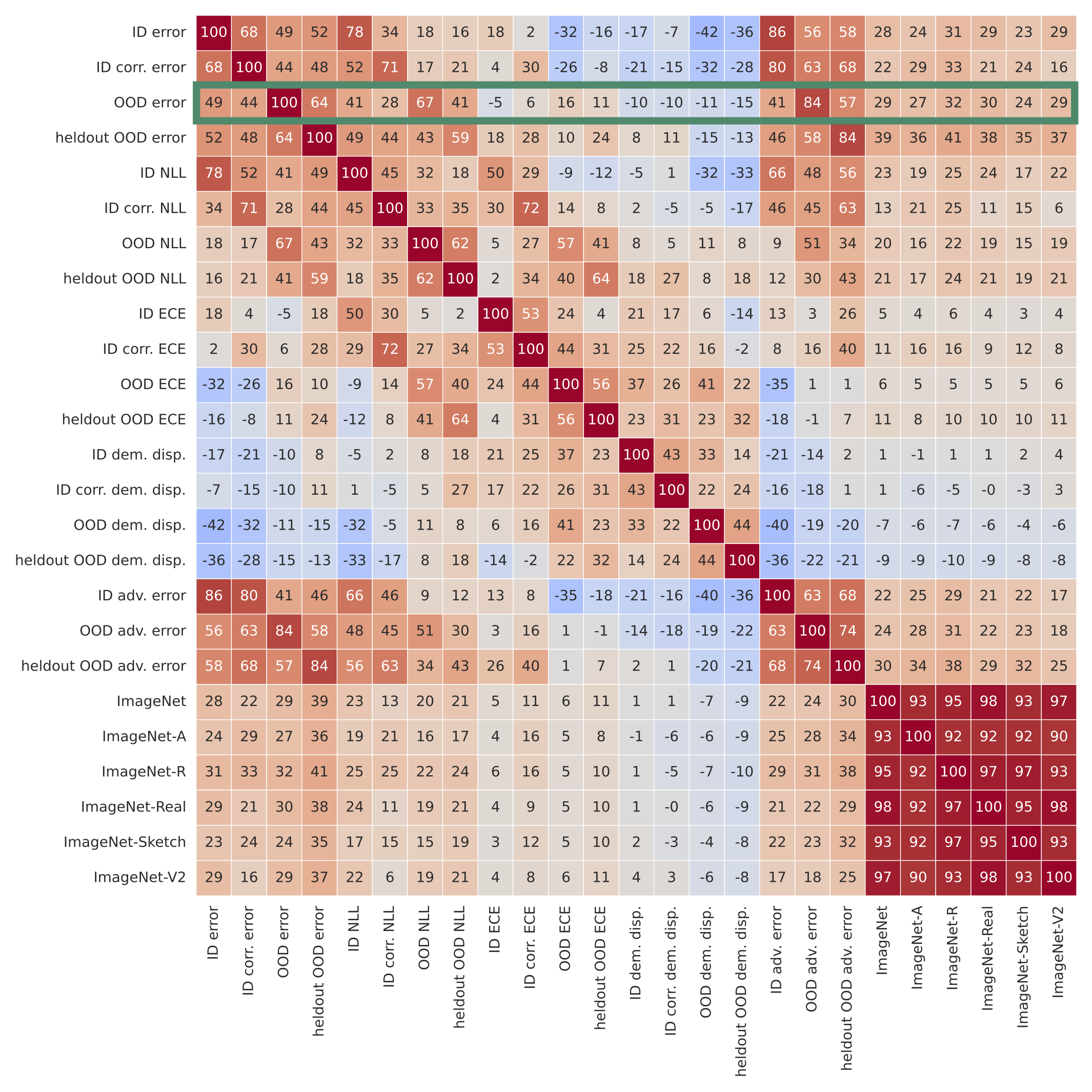
Figure S1: Rank correlation matrix averaged over all tasks. The matrix shows the predictiveness of a metric (either evaluated on ID data, ID corrupted data, OOD, held-out OOD data or ImageNet) of another metric. Positive values indicate a positive link between the metrics, i.e. better results for one metric tend to lead to better results for the other metric. Negative values indicate a negative link, i.e. better results for one metric tend to lead to worse results for the other metric. All averaged correlation coefficients are multiplied by a factor of $100$ for better readability. As an example, the highlighted green rectangle shows how well metrics predict OOD classification error, this information is shown separately as a bar plot in Fig. 3 (red bars) in the main text.

A.3 Analyzing each task separately

In Section 4.2 in the main text we argue that out-of-distribution generalization has many facets. Some patterns observed in prior work actually only hold on a subsets of the tasks included in our study. To investigate the stability of observations across different tasks we compute the averaged correlation matrices for each task separately. For each task, we only include the datasets that belong to that tasks (see Appendix E) and show the matrices in Figs. S2 and S3.

Some observations are stable across all tasks (e.g., classification error is always the strongest predictors on ID and held-out data, respectively). For other metrics we observe large variability across tasks. For instance for some tasks, demographic disparity has a strong positive link to OOD accuracy, for others it is reversed (i.e., here lower demographic disparity leads to a higher classification error). This also holds for calibration error. We marked the according cells in the task-specific correlation matrices with a green square. We also observe mixed positive and negative links for multi-domain calibration (held-out OOD ECE, marked by yellow squares in the plots). This is in contrast to the claims by [109] that multi-domain calibration is generally a good indicator for OOD robustness since it actually only holds on a subset of the tasks.

A.4 Analyzing each shift type separately

In this section we investigate how results change for different shift types. We define the shift type based on ID dataset regime and the OOD dataset regime as follows. First, we label each dataset by one of the domain types artificial and real, see Table S1. For instances, the label artificial refers to datasets of images composed from sketches, clipart or simulated environments. Second, for an (ID, OOD) dataset pair the shift is derived by the ID (source) domain type and the OOD (target) domain type. E.g., the dataset pair: (OfficeHome-ClipArt, OfficeHome-RealWorld) is labeled by the shift type artificial $\rightarrow$ real.

Similarly, as in Section A.3, we compute the averaged correlation matrix for the subset of dataset pairs corresponding to each shift type separately. The matrices are displayed in the figures Fig. S4. For instance, for the shift type artificial $\rightarrow$ real, corruption metrics are more predictive of OOD accuracy then for the reversed shift type real $\rightarrow$ artificial, see the highlighted green cells in the plots.

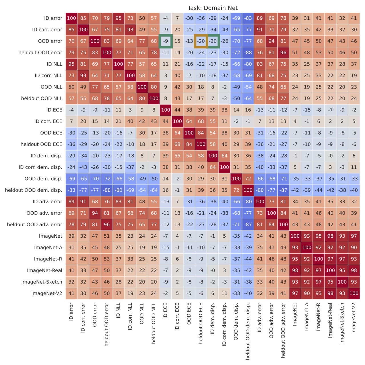
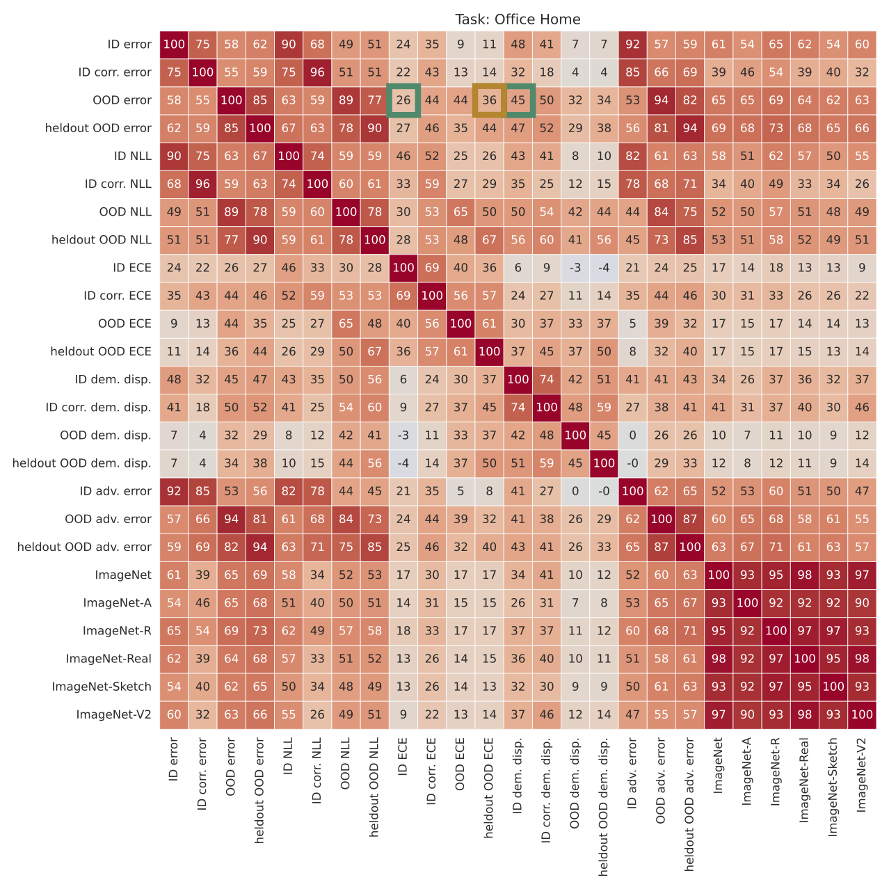
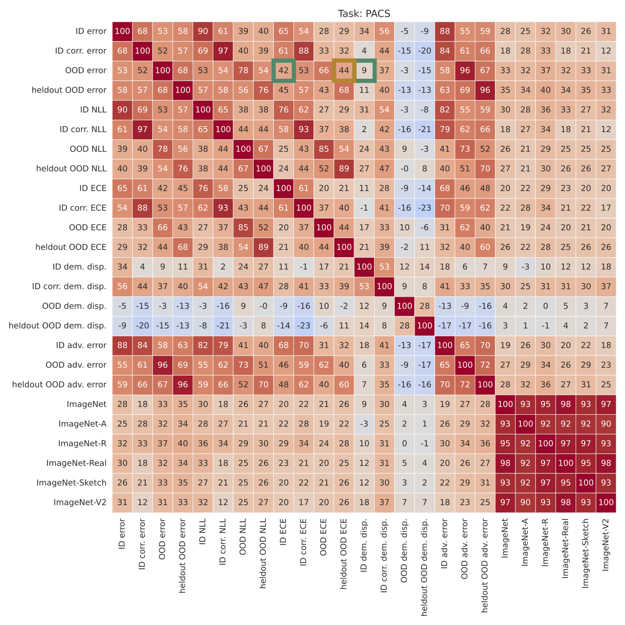
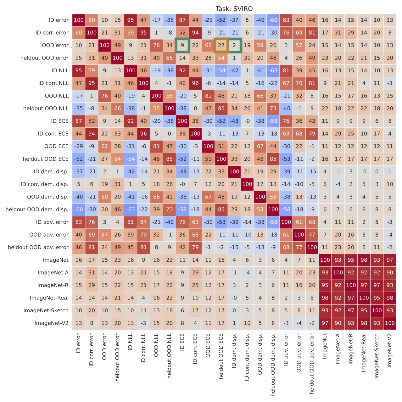
Figure S2: Averaged correlation matrices for each task separately. For each task we only consider the corresponding datasets and compute the correlation coefficients separately. We highlight differences between tasks for ID demographic disparity, ID calibration with green squares and differences for held-out ECE with yellow squares.

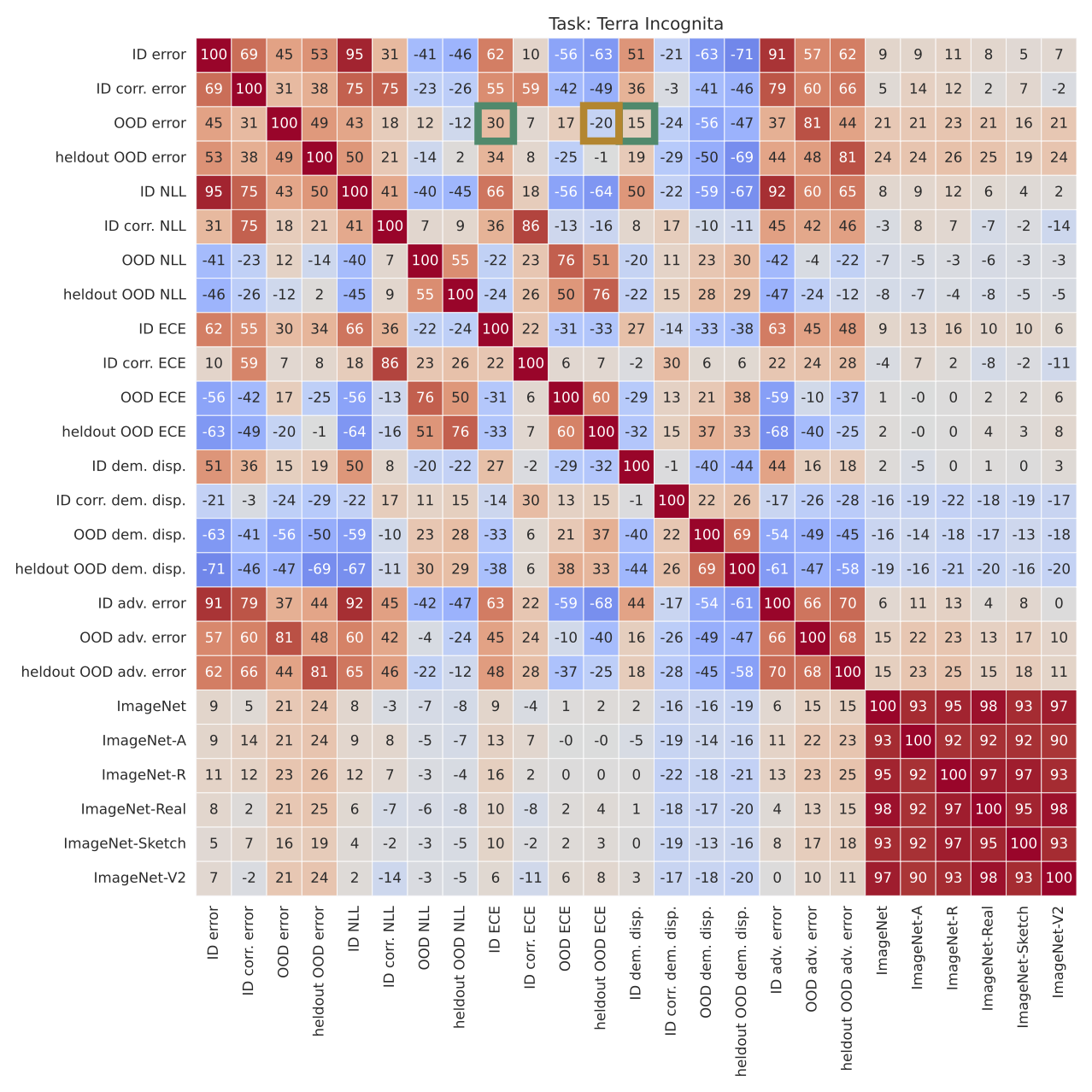
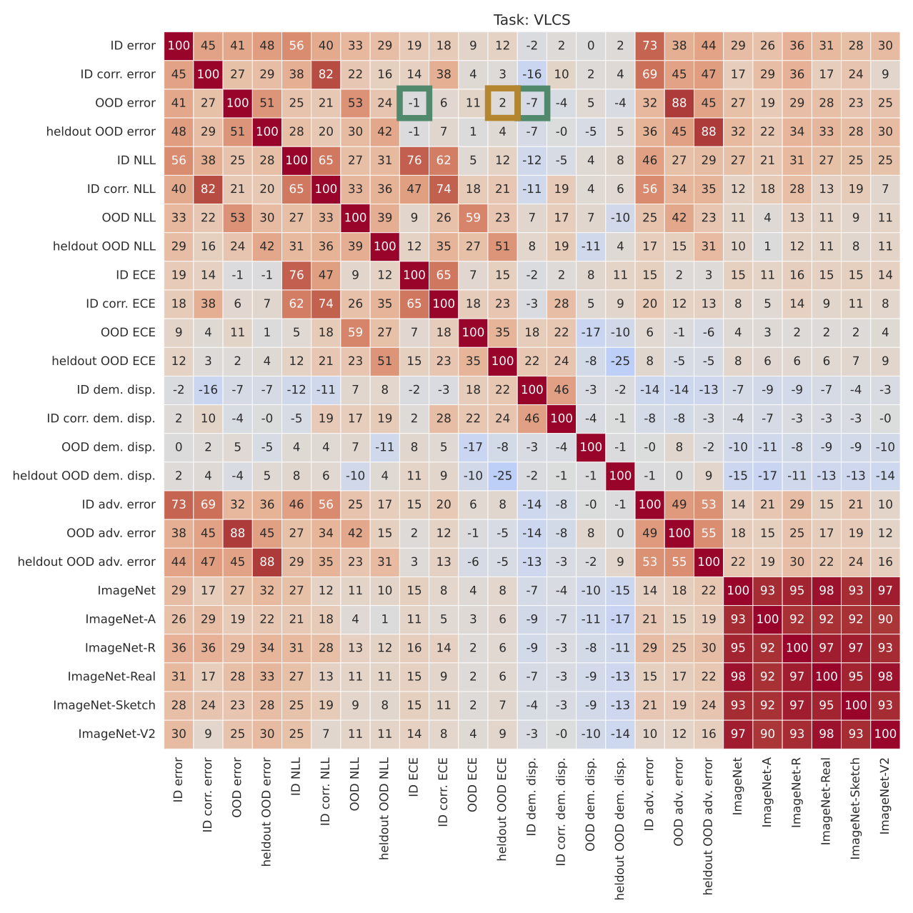
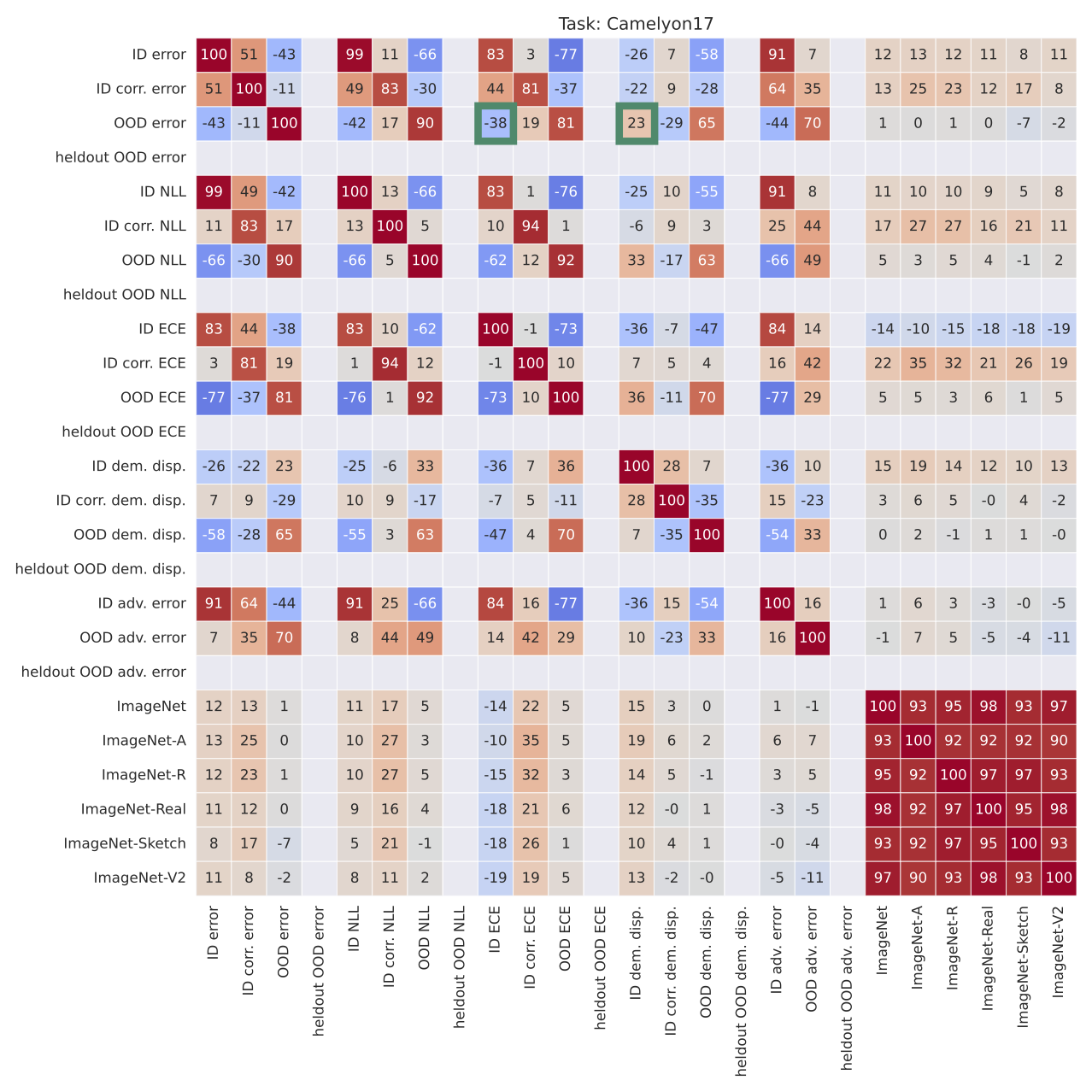
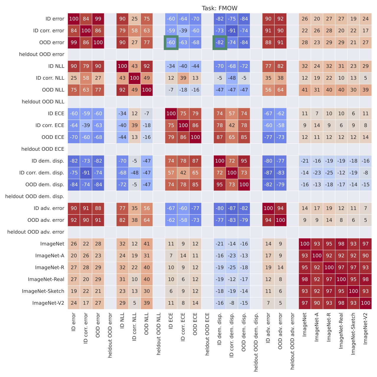
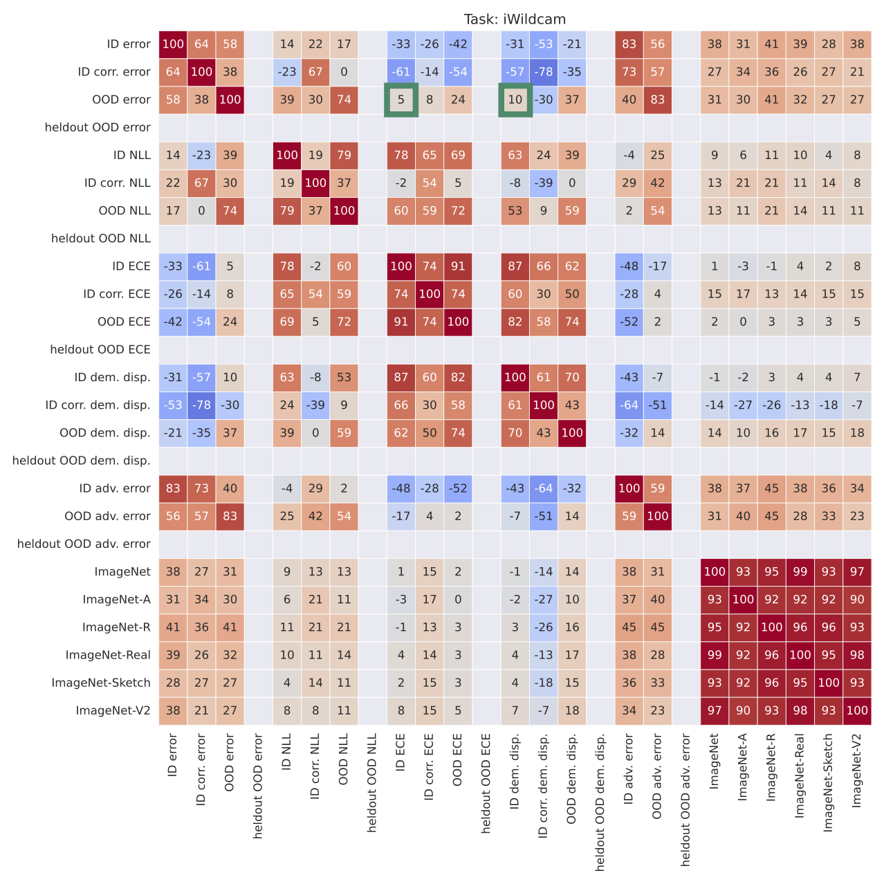
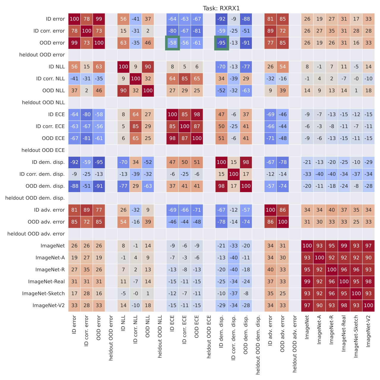
Figure S3: Averaged correlation matrices for each task separately (continued). We highlight differences between tasks for ID demographic disparity, ID calibration with green squares and differences for held-out ECE with yellow squares. Note that for the tasks Camelyon17, FMOW, iWildcam and RXRX1, no held-out OOD data is available (i.e., only one OOD split is provided).

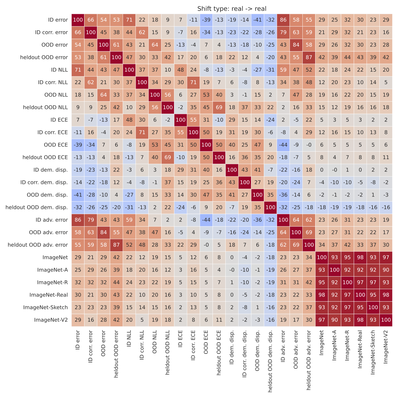
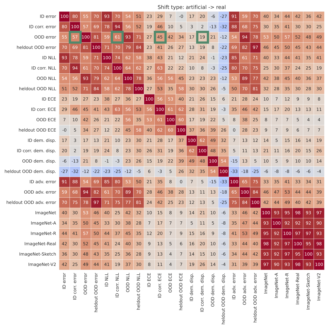
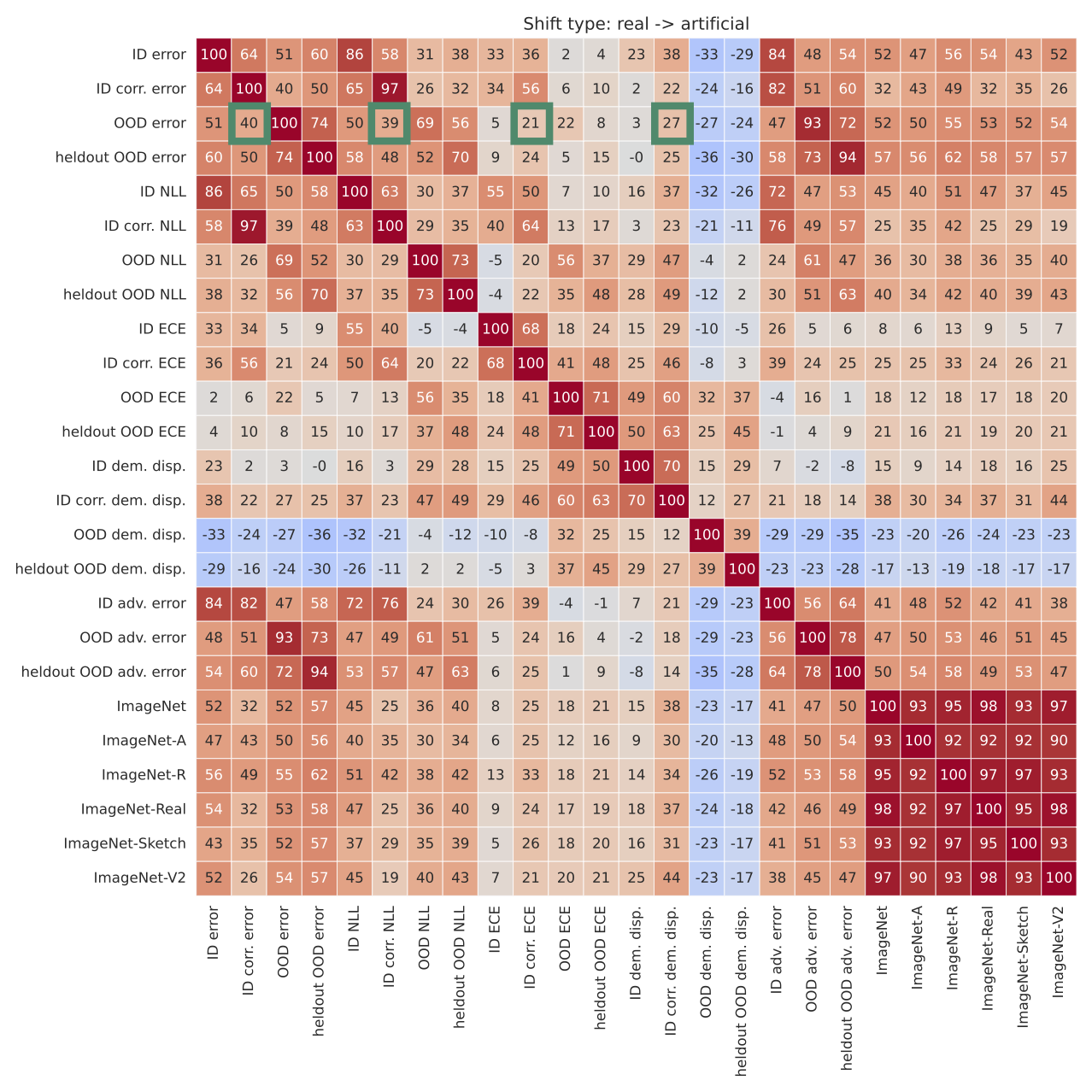
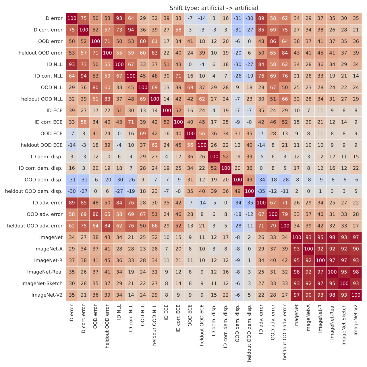
Figure S4: Averaged correlation matrices for each shift type separately. The shift types are defined based on the source and target domain, see Table S1. Using green squares we highlight differences of the corruption metrics predicting OOD accuracy for the shift types real $\rightarrow$ artificial and artificial $\rightarrow$ real.

Appendix B Factor analysis: details and background

This section gives a short introduction to factor analysis, provides details about the data and the pre-processing used for the factor analysis of Section 4.1 and presents the data’s scree plot in Fig. S5.

Background.

Factor analysis is a well-established tool from statistics used to analyze tabular data, such as data arising from a poll, where the columns would be the questions and the rows the answers of each individual. It aims at finding a minimal amount of latent variables called factors that suffice to explain the data and reflect the main dependencies between columns. In particular, given $k$ factors $f_{1},f_{2},\ldots,f_{k}$, each column $c_{i}$ gets approximated as $c_{i}=\lambda_{i1}f_{1}+\cdots\lambda_{ik}f_{k}$ where the $\lambda_{ij}$s are called factor loadings. Because columns get standardized prior to the analysis and factors are scaled to have unit norm, the loadings lie between $-1$ and $1$. While the factors are a priori abstract variables with no pre-defined interpretation, one of the main challenges and goals of factor analysis is to understand what variability they capture by analyzing their loadings. Note that the first $k$ factors span the subspace defined by the first $k$ eigenvectors of the data matrix. However, the factors themselves are only defined up to a rotation, since rotating the factors and the loadings accordingly, the $c_{i}$s remain unchanged. Some rotations lead to factors whose loadings are easier to interpret than others. Therefore, the typical workflow of a factor analysis is as follows. (1) Decompose the data into eigenvectors and use the eigenvalues to choose the number $k$ of factors to keep. The simplest rule of thumb is to keep all eigenvectors with eigenvalues $\geq$ 1. (2) Try out different rotations of the $k$ first eigenvectors, to make the loadings as easy as possible to explain or interpret. To do so, one typically just tests several standard rotation methods such as the varimax, quartimax, or equamax methods (which typically try to promote some form of sparse loadings). (3) Interpret the obtained factors and conclude on the relations between the columns that they show.

Data preprocessing.

We organize our data in a table with rows being fine-tuned networks and columns the metrics. Specifically, each network is defined by its model architecture, the adaptation dataset used for fine-tuning and the training parameters (augmentation strategy, learning rate, number of training epochs, and fine-tuning method), leading in theory to a total of $7776$ networks ($9$ architectures $\times$ $36$ datasets $\times$ $3\cdot 2\cdot 2\cdot 2$ parameters). Note that we considered only those networks finetuned on full datasets, ignoring the few-shot data. For each network, we considered a total of $16$ metrics: the $6$ base metrics (cf. Section 2) computed respectively on the held-out test data from the adaptation domain (the in-distribution metrics), on its corrupted variant (except adversarial accuracy, which we did not compute on corrupted data), and, for each metric, its average over all out-of-distribution datasets from the adaptation dataset’s task. Concerning the log-likelihood metric, most values lied between $0$ and $5$, but some outliers could take values up to $1\mathrm{e}{10}$. We therefore mapped all log-likelihood values through the following function: $f(x)=10(1-\exp(-\nicefrac{{x}}{{10}}))$. Doing so ensures that all typical log-likelihood values remain nearly unchanged up to a rescaling factor ($f$ is almost linear in $0$), while bigger values saturate at $10$. We used python’s factor_analyzer package for the analysis.

Factor analysis and factor loading plot.

The scree plot in Fig. S5 shows the eigenvalues of the data in decreasing order. We decided to retain $4$ factors, since only $4$ eigenvalues were $\geq 1$. We then used the equamax rotation method, but the results do not change significantly with other standard methods. The factor loadings for each metric are shown in Fig. 1 in the main text and discussed there (see Section 4.1).

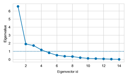
Figure S5: Scree plot: Eigenvalues of the standardized data from the factor analysis, sorted by decreasing order of magnitude. As explained in Section 4.1, we decided to take the first $4$ factors, since only the first $4$ eigenvalues are above the usual threshold value of $1$.

Appendix C Detailed analysis on the effect of the fine-tuning and augmentation strategies

In the following we provide additional studies on the effect of the augmentation and fine-tuning method on the ID and OOD performance. The main results are summarized in the main text in Section 5.

C.1 The effect of the fine-tuning strategy

Fig. S6 shows the average ID and OOD accuracy for the two considered fine-tuning strategies: fine-tuning the full architecture and the linear probe classifier (fine-tuning the head only). To make the difference of both strategies more clear we show the normalized accuracy gap of both fine-tuning approaches in Fig. S7. The gap is computed by

$$\textrm{gap}=\frac{\textrm{acc}_{\textrm{full}}-\textrm{acc}_{\textrm{head only}}}{\textrm{acc}_{\textrm{full}}},$$ (S1)

where the accuracy terms are averaged over all datasets within a task. We find that fine-tuning the full architecture is usually superior when using the full fine-tuning dataset. Interestingly, when having access to less data (especially in the few-shot-10 setting), we observe that the linear probe classifier can be better, especially when evaluating on OOD data. This may confirm the idea that changing the last layer only leads to a higher inductive bias by the pre-training data. This is particularly beneficial in low-data regimes when generalizing to OOD data. This insights are in line with previous work (e.g., [120], Fig. 4).

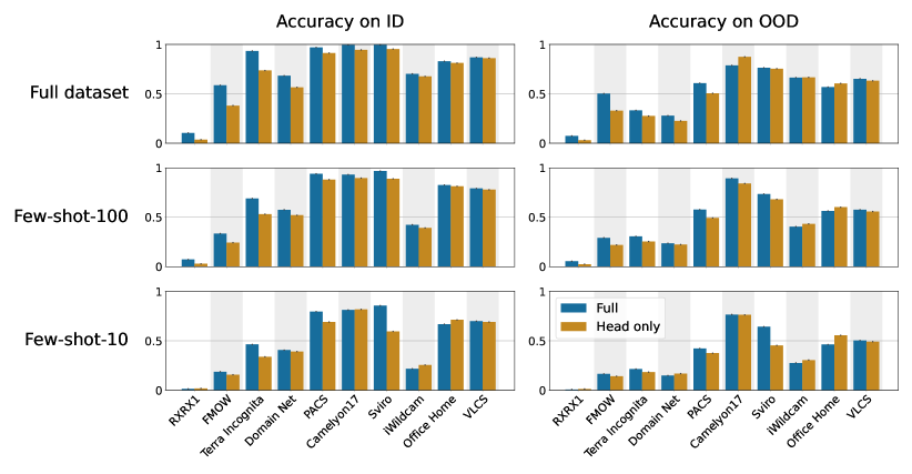
Figure S6: Each bar plot shows the average ID (left) and OOD accuracy (right) obtained by fine-tuning the full architecture or the head only. We compare the results in the setting of training on the full dataset and the few-shot settings (columns). In all plots, the black bars (which are very small and hence barely visible) indicate the standard error.

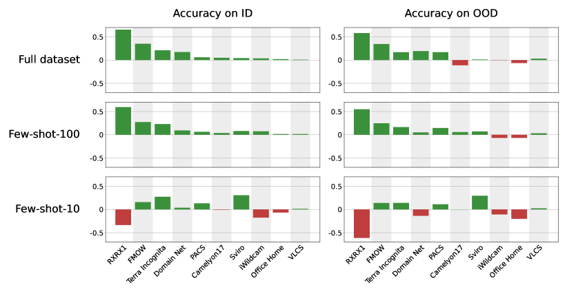
Figure S7: Each bar plot shows the normalized accuracy gap between fine-tuning the full architecture or the head only. We report the average ID (left) and OOD (right) accuracy in setting of training on the full dataset and the few-shot settings (columns). In the low data regime fine-tuning the head only can be beneficial, especially for OOD accuracy.

C.2 The effect of the augmentation strategy

In addition to Fig. 5 in the main text, we report the average ID and OOD accuracy for each augmentation method for each tasks separately. We do not observe a significant difference between the tasks.

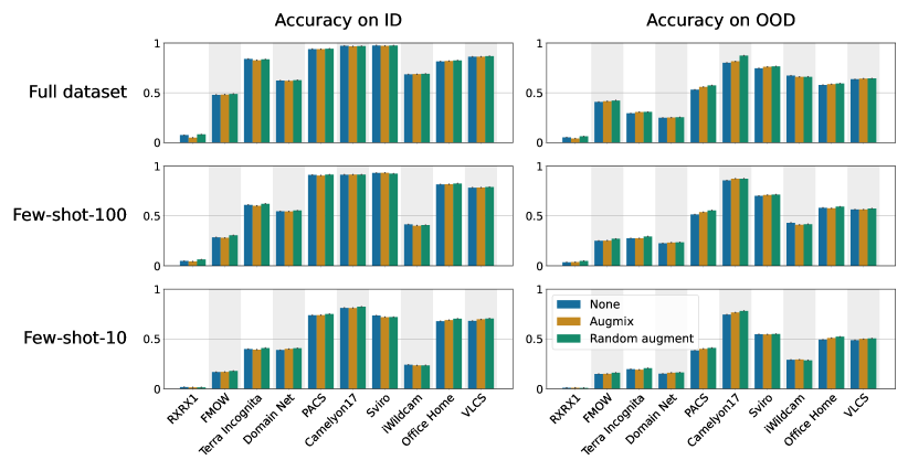
Figure S8: Each bar plot shows the average ID (left) and OOD accuracy (right) obtained by using the different augmentation strategies. We compare the results in the setting of training on the full dataset and the few-shot settings (columns). In all plots, the black bars (which are very small and hence barely visible) indicate the standard error.

Appendix D Detailed scatter plots for the relationship of ID vs. OOD accuracy

Figure 2 in the main text shows four prototypical patterns of ID versus OOD accuracy plots, taken from four exemplary dataset pairs out of the $172$ dataset pairs considered in this study. This section now shows all $172$ ID-vs-OOD-accuracy scatter plots in Fig. S9, grouped by task. Each column corresponds to one adaptation (i.e., fine-tuning) dataset. Interestingly, the exemplary scatter plot patterns described in Fig. 2 (functional relationship, vertical line/underspecification, no generalization/ horizontal line, and random generalization/point-cloud) appear to be essentially task related. For example, in OfficeHome and DomainNet, almost all (ID, OOD) dataset pairs exhibit a clear functional relationship. In Terra Incognita, generalization never works (horizontal line) or is near-random (unstructured point cloud). The SVIRO dataset pairs almost systematically fall into the underspecification/vertical line category, and PACS and VLCS exhibit either a relatively clear functional relationships or an underspecification pattern (vertical line).

For better readability, the plots do not include all degrees of freedom of our study. Specifically, we plot only those networks that were trained on the full adaptation dataset (i.e., we do not include the few-shot settings) and focus on the fine-tuning strategy where all weights of the network get fine-tuned (in contrast to fine-tuning the head only).

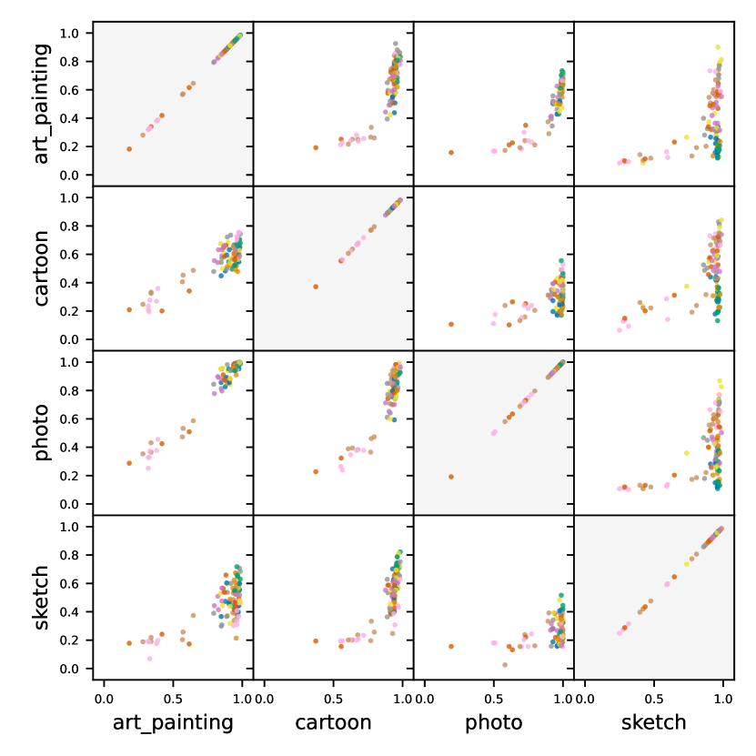
(a) PACS: We observe either a clear functional relationships or an “underspecified” regime (vertical line).

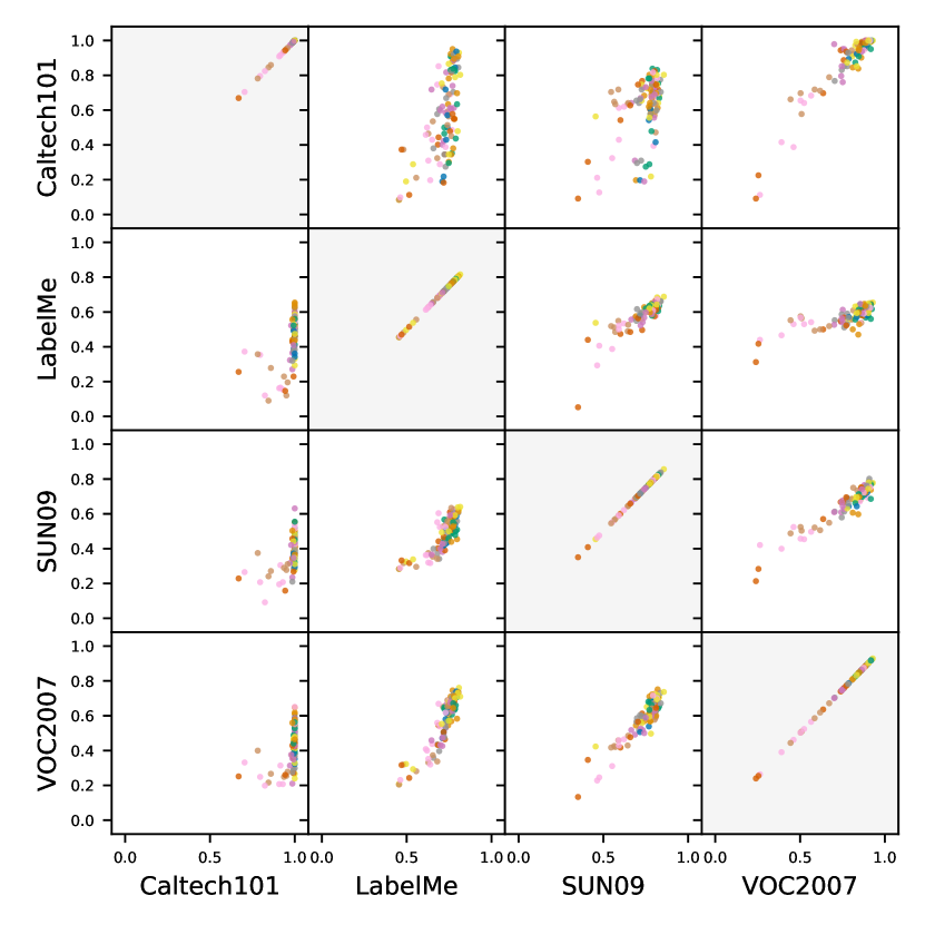
(b) VLCS: We observe similar patterns as for PACS.

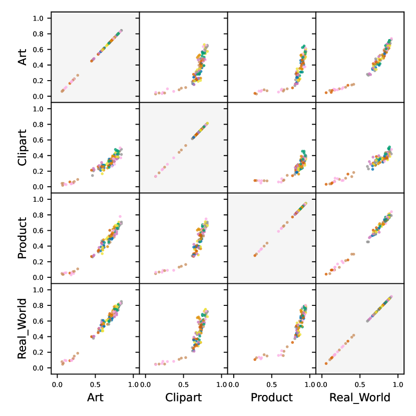
(c) Office Home: For all dataset pairs we observe clear functional relationships.

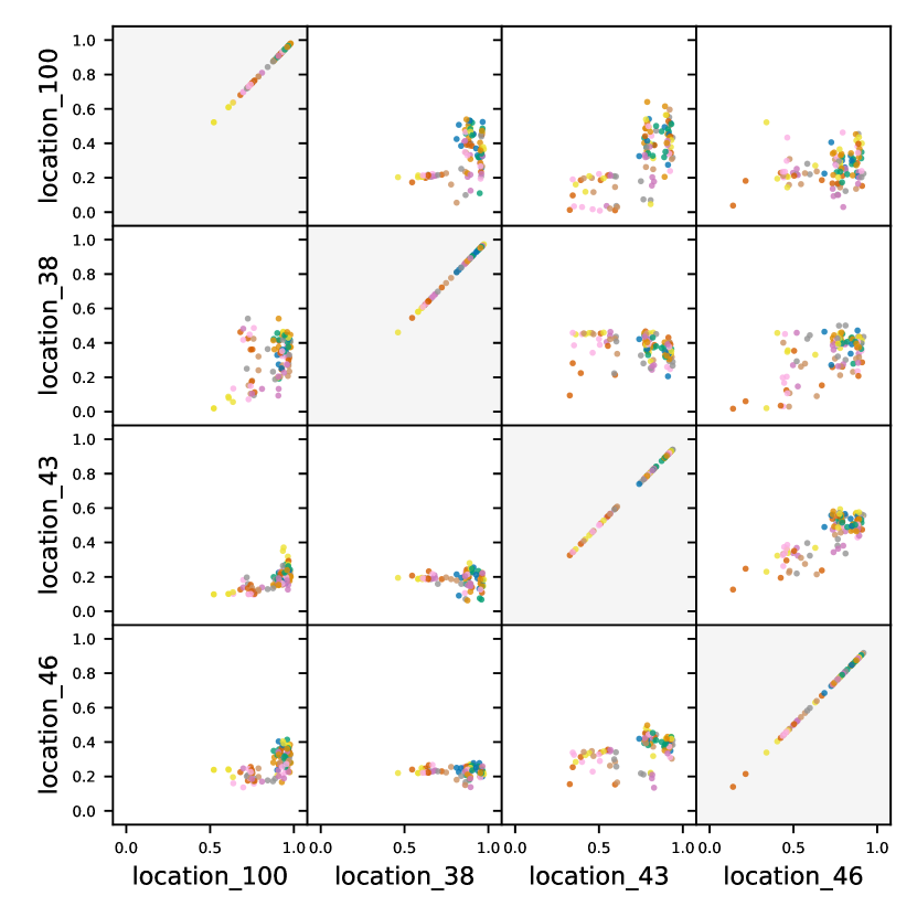
(d) Terra Incognita: Either no transfer (horizontal line) or random associations (scattered point cloud).

Figure S9: ID versus OOD accuracy for various tasks and dataset pairs. Every point represents one fine-tuned network. The domains on the x-axis are the ones used for fine-tuning and measuring the ID test accuracy. The datasets on the y-axis are the OOD datasets. We plot only networks that were trained on the full dataset (no few-shot datasets) and with all their weights (no head-only fine-tuning). All points in a same column with the same x-axis value represent the same fine-tuned network. Interestingly, the different patterns described in Fig. 2 (clear functional relationship, underspecification / vertical line, no generalization / horizontal line, random generalization / point-cloud) appear to be essentially task dependent. The reader may want to focus on the regions with higher point densities, since the networks outside those denser regions typically correspond to a suboptimal combination of hyperparameters that did not allow to reach convergence.

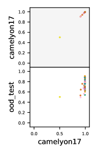
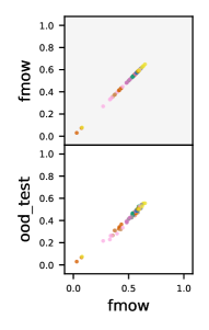
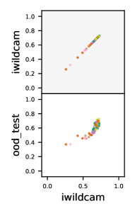
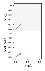
(a) WILDS Camelyon17, FMoW, iWildCam, RXRX1: We observe underspecification (Camelyon17) or clear functional relationships (others).

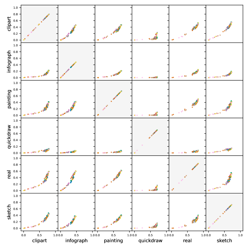
(b) Domain Net: For all dataset pairs we observe clear functional relationships.

Figure S10: (Continued) ID vs OOD accuracy for various tasks and dataset pairs. For a longer caption, see previous page.

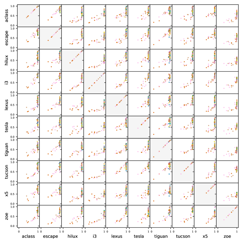
(a) SVIRO: almost always underspecified regime (vertical line).

Figure S11: (Continued) ID vs OOD accuracy for various tasks and dataset pairs. For a longer caption, see previous page.

Appendix E Details on the tasks and datasets

We use 36 datasets collected from different benchmarks: DomainNet [79], PACS [56], SVIRO [26], Terra Incognita [13] as well as the Caltech101 [34], VLCS [104], Sun09 [18], VOC2007 [32] and the Wilds datasets [51]. We group the domains (datasets) into ten different tasks, see Table S1 list. For all tasks besides the wilds tasks, we consider all possible (ID, OOD) dataset pairs, i.e., we fine-tune on one dataset in the task (ID dataset) and evaluate the model on all the others (which are considered to be the OOD datasets). For the Wilds datasets we use the predefined ID and OOD splits.

Table S1: Overview over tasks and their associated domains (datasets), along with a domain type tag.

Task	Domain	Domain type
PACS	art_painting	Artificial
	cartoon	Artificial
	photo	Real
	sketch	Artificial
VLCS	Caltech101	Real
	LabelMe	Real
	SUN09	Real
	VOC2007	Real
domain_net	clipart	Artificial
	infograph	Artificial
	painting	Artificial
	quickdraw	Artificial
	real	Real
	sketch	Artificial
office_home	Art	Artificial
	Clipart	Artificial
	Product	Real
	Real_World	Real
sviro	aclass	Artificial
	escape	Artificial
	hilux	Artificial
	i3	Artificial
	lexus	Artificial
	tesla	Artificial
	tiguan	Artificial
	tucson	Artificial
	x5	Artificial
	zoe	Artificial
terra_incognita	location_100	Real
	location_38	Real
	location_43	Real
	location_46	Real
wilds-camelyon17	camelyon17-id	Real
	camelyon17-ood	Real
wilds-fmow	fmow-id	Real
	fmow-ood	Real
wilds-iwildcam	iwildcam-id	Real
	iwildcam-ood	Real
wilds-rxrx1	rxrx1-id	Real
	rxrx1-ood	Real

E.1 Comparison of the task difficulty

In the following we discuss the difficulty of the different tasks. In our context, the difficulty of a task might be defined by how hard it is to transfer from the ID dataset to the OOD dataset. In other words, a task is more difficult if the distribution of the OOD data is more distant from the distribution of the ID data. It is not obvious how to measure this distance and multiple approaches have been proposed [e.g., 15, 122]. Here we choose a more direct measure and compare the ID and OOD performance for each task averaged over all dataset pairs in the task, and all models and training hyperparameters. Fig. S12 shows the average accuracy obtained on all datasets within each task. In the top plot we compare the average ID accuracy and OOD accuracy. In the bottom plot we display the normalized ID vs. OOD accuracy gap computed by

$$\textrm{gap}=\frac{\textrm{acc}_{\textrm{ID}}-\textrm{acc}_{\textrm{OOD}}}{\textrm{acc}_{\textrm{ID}}},$$ (S2)

where the accuracy terms are averaged over all datasets within a task. The average ID vs. OOD accuracy gap can serve as a proxy measure of the difficulty of a task. It indicates how hard the OOD prediction task is in average for a model that was trained on the ID data.

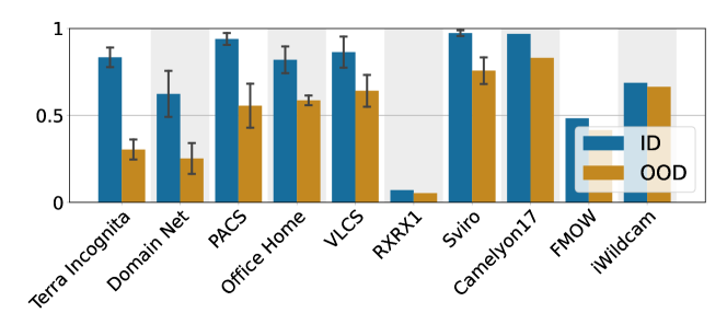
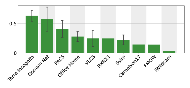
Figure S12: top: Mean accuracy on ID data and OOD data for each task (averaged over all datasets in the task, architectures, augmentation and fine-tuning strategies, c.f. Table S1). bottom: Normalized mean ID vs. OOD accuracy gap for each task, see Eq. S2. This indicates the average difficulty of the domain generalization. In all plots, the black bars indicate the standard deviation (not the standard error as in the other plots) across the datasets within the task if the tasks contains multiple dataset pairs.

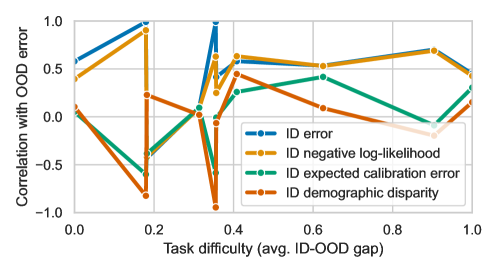
Figure S13: Each line shows the correlation coefficients between an ID metric and the OOD prediction error as a function of task difficulty. The task difficulty was computed by the normalized ID vs. OOD gap as shown in Fig. S12 and was linearly mapped to values between 0 and 1. No clear pattern is visible and the correlation coefficients seem to be rather independent of the task difficulty.

Next we discuss how the predictiveness of the different metrics depend on the task difficulty. Fig. S13 shows the correlation coefficients (between the ID metrics and OOD prediction error) as a function of task difficulty. We observe that ID error is the best predictor of the ID error for most difficulty levels. Besides this observation we find that the results are noisy and no clear pattern can be observed. Surprisingly, the correlation coefficients seem to be rather independent of the task difficulty.

Appendix F Detailed comparison of model performances

We compare the in-distribution (ID) and out-of-distribution (OOD) performance for each model on all tasks. Here we follow the scenario where the hyperparameters are selected on an held-out ID validation split (this mimics the usual hyperparameter selection approach used in practice). We then compute the ID performance on the ID test set and the mean OOD performance on all other (OOD) domains of a task. Finally, we report the mean ID and OOD accuracy within each task and the gap between ID and OOD performance in LABEL:tab:model_comparison. The numbers in gray represent the standard error of these means. This table represents a more details view on the performance of each individual model compared to Table 2 in the main text, where the performance is averaged over tasks.

Table S2: Average ID and OOD accuracy of each model on each task over all domains in the task.

Model	Domain	ID Error	OOD Error	OOD-ID Gap
Deit	PACS	0.033 $\pm$ 0.003	0.333 $\pm$ 0.022	0.299 $\pm$ 0.023
	VLCS	0.118 $\pm$ 0.010	0.328 $\pm$ 0.017	0.210 $\pm$ 0.022
	domain_net	0.316 $\pm$ 0.009	0.703 $\pm$ 0.014	0.387 $\pm$ 0.017
	office_home	0.131 $\pm$ 0.008	0.341 $\pm$ 0.017	0.209 $\pm$ 0.020
	sviro	0.014 $\pm$ 0.001	0.219 $\pm$ 0.005	0.205 $\pm$ 0.005
	terra_incognita	0.127 $\pm$ 0.011	0.661 $\pm$ 0.013	0.533 $\pm$ 0.020
	wilds-camelyon17	0.022 $\pm$ 0.007	0.156 $\pm$ 0.036	0.134 $\pm$ 0.040
	wilds-fmow	0.468 $\pm$ 0.036	0.543 $\pm$ 0.030	0.074 $\pm$ 0.007
	wilds-iwildcam	0.275 $\pm$ 0.007	0.289 $\pm$ 0.009	0.014 $\pm$ 0.006
	wilds-rxrx1	0.925 $\pm$ 0.005	0.939 $\pm$ 0.004	0.014 $\pm$ 0.002
DenseNet169	PACS	0.061 $\pm$ 0.006	0.523 $\pm$ 0.031	0.463 $\pm$ 0.031
	VLCS	0.137 $\pm$ 0.011	0.365 $\pm$ 0.018	0.228 $\pm$ 0.024
	domain_net	0.387 $\pm$ 0.011	0.788 $\pm$ 0.012	0.401 $\pm$ 0.015
	office_home	0.209 $\pm$ 0.010	0.496 $\pm$ 0.017	0.287 $\pm$ 0.019
	sviro	0.047 $\pm$ 0.003	0.274 $\pm$ 0.005	0.227 $\pm$ 0.006
	terra_incognita	0.186 $\pm$ 0.015	0.725 $\pm$ 0.015	0.539 $\pm$ 0.019
	wilds-camelyon17	0.036 $\pm$ 0.012	0.169 $\pm$ 0.038	0.133 $\pm$ 0.047
	wilds-fmow	0.526 $\pm$ 0.046	0.593 $\pm$ 0.037	0.067 $\pm$ 0.009
	wilds-iwildcam	0.319 $\pm$ 0.010	0.364 $\pm$ 0.012	0.046 $\pm$ 0.021
	wilds-rxrx1	0.911 $\pm$ 0.039	0.937 $\pm$ 0.027	0.026 $\pm$ 0.014
EfficientNet2	PACS	0.053 $\pm$ 0.005	0.469 $\pm$ 0.032	0.416 $\pm$ 0.032
	VLCS	0.140 $\pm$ 0.012	0.374 $\pm$ 0.018	0.234 $\pm$ 0.023
	domain_net	0.369 $\pm$ 0.012	0.734 $\pm$ 0.014	0.365 $\pm$ 0.017
	office_home	0.172 $\pm$ 0.009	0.403 $\pm$ 0.015	0.230 $\pm$ 0.017
	sviro	0.031 $\pm$ 0.002	0.249 $\pm$ 0.005	0.218 $\pm$ 0.005
	terra_incognita	0.187 $\pm$ 0.016	0.703 $\pm$ 0.013	0.516 $\pm$ 0.017
	wilds-camelyon17	0.039 $\pm$ 0.015	0.194 $\pm$ 0.039	0.155 $\pm$ 0.049
	wilds-fmow	0.530 $\pm$ 0.053	0.588 $\pm$ 0.047	0.059 $\pm$ 0.006
	wilds-iwildcam	0.325 $\pm$ 0.022	0.383 $\pm$ 0.017	0.058 $\pm$ 0.009
	wilds-rxrx1	0.901 $\pm$ 0.032	0.927 $\pm$ 0.022	0.025 $\pm$ 0.013
GMLP	PACS	0.070 $\pm$ 0.007	0.434 $\pm$ 0.026	0.363 $\pm$ 0.027
	VLCS	0.136 $\pm$ 0.011	0.361 $\pm$ 0.016	0.225 $\pm$ 0.022
	domain_net	0.404 $\pm$ 0.012	0.753 $\pm$ 0.013	0.348 $\pm$ 0.017
	office_home	0.195 $\pm$ 0.009	0.409 $\pm$ 0.016	0.214 $\pm$ 0.020
	sviro	0.034 $\pm$ 0.002	0.260 $\pm$ 0.006	0.226 $\pm$ 0.006
	terra_incognita	0.180 $\pm$ 0.016	0.708 $\pm$ 0.010	0.528 $\pm$ 0.021
	wilds-camelyon17	0.041 $\pm$ 0.016	0.214 $\pm$ 0.032	0.173 $\pm$ 0.042
	wilds-fmow	0.556 $\pm$ 0.056	0.624 $\pm$ 0.046	0.069 $\pm$ 0.011
	wilds-iwildcam	0.338 $\pm$ 0.009	0.329 $\pm$ 0.006	-0.008 $\pm$ 0.011
	wilds-rxrx1	0.972 $\pm$ 0.008	0.977 $\pm$ 0.006	0.005 $\pm$ 0.002
Mixer	PACS	0.091 $\pm$ 0.009	0.469 $\pm$ 0.028	0.378 $\pm$ 0.029
	VLCS	0.150 $\pm$ 0.011	0.386 $\pm$ 0.017	0.236 $\pm$ 0.022
	domain_net	0.433 $\pm$ 0.014	0.785 $\pm$ 0.012	0.352 $\pm$ 0.016
	office_home	0.215 $\pm$ 0.011	0.472 $\pm$ 0.016	0.257 $\pm$ 0.020
	sviro	0.023 $\pm$ 0.001	0.251 $\pm$ 0.005	0.228 $\pm$ 0.005
	terra_incognita	0.172 $\pm$ 0.015	0.737 $\pm$ 0.013	0.565 $\pm$ 0.018
	wilds-camelyon17	0.025 $\pm$ 0.008	0.154 $\pm$ 0.029	0.129 $\pm$ 0.036
	wilds-fmow	0.534 $\pm$ 0.042	0.608 $\pm$ 0.038	0.074 $\pm$ 0.005
	wilds-iwildcam	0.333 $\pm$ 0.005	0.374 $\pm$ 0.009	0.041 $\pm$ 0.012
	wilds-rxrx1	0.983 $\pm$ 0.006	0.985 $\pm$ 0.005	0.002 $\pm$ 0.001
ResMLP	PACS	0.066 $\pm$ 0.006	0.465 $\pm$ 0.026	0.398 $\pm$ 0.026
	VLCS	0.145 $\pm$ 0.011	0.395 $\pm$ 0.017	0.250 $\pm$ 0.022
	domain_net	0.398 $\pm$ 0.011	0.764 $\pm$ 0.012	0.367 $\pm$ 0.016
	office_home	0.203 $\pm$ 0.010	0.453 $\pm$ 0.018	0.250 $\pm$ 0.021
	sviro	0.027 $\pm$ 0.001	0.245 $\pm$ 0.005	0.218 $\pm$ 0.005
	terra_incognita	0.164 $\pm$ 0.014	0.694 $\pm$ 0.013	0.530 $\pm$ 0.020
	wilds-camelyon17	0.032 $\pm$ 0.012	0.157 $\pm$ 0.015	0.125 $\pm$ 0.025
	wilds-fmow	0.544 $\pm$ 0.047	0.613 $\pm$ 0.039	0.069 $\pm$ 0.009
	wilds-iwildcam	0.317 $\pm$ 0.006	0.343 $\pm$ 0.009	0.026 $\pm$ 0.008
	wilds-rxrx1	0.949 $\pm$ 0.010	0.959 $\pm$ 0.005	0.010 $\pm$ 0.005
ResNet50	PACS	0.054 $\pm$ 0.005	0.499 $\pm$ 0.032	0.445 $\pm$ 0.033
	VLCS	0.137 $\pm$ 0.011	0.325 $\pm$ 0.017	0.189 $\pm$ 0.022
	domain_net	0.359 $\pm$ 0.011	0.749 $\pm$ 0.014	0.390 $\pm$ 0.016
	office_home	0.180 $\pm$ 0.010	0.431 $\pm$ 0.017	0.251 $\pm$ 0.020
	sviro	0.025 $\pm$ 0.001	0.244 $\pm$ 0.005	0.220 $\pm$ 0.006
	terra_incognita	0.176 $\pm$ 0.014	0.698 $\pm$ 0.015	0.521 $\pm$ 0.019
	wilds-camelyon17	0.036 $\pm$ 0.013	0.195 $\pm$ 0.045	0.159 $\pm$ 0.052
	wilds-fmow	0.512 $\pm$ 0.045	0.579 $\pm$ 0.036	0.067 $\pm$ 0.010
	wilds-iwildcam	0.313 $\pm$ 0.015	0.328 $\pm$ 0.007	0.015 $\pm$ 0.010
	wilds-rxrx1	0.894 $\pm$ 0.032	0.925 $\pm$ 0.021	0.030 $\pm$ 0.012
Swin	PACS	0.048 $\pm$ 0.006	0.393 $\pm$ 0.027	0.345 $\pm$ 0.027
	VLCS	0.121 $\pm$ 0.010	0.350 $\pm$ 0.017	0.230 $\pm$ 0.021
	domain_net	0.340 $\pm$ 0.010	0.718 $\pm$ 0.014	0.378 $\pm$ 0.017
	office_home	0.152 $\pm$ 0.009	0.351 $\pm$ 0.018	0.199 $\pm$ 0.022
	sviro	0.019 $\pm$ 0.001	0.218 $\pm$ 0.005	0.199 $\pm$ 0.005
	terra_incognita	0.144 $\pm$ 0.012	0.643 $\pm$ 0.013	0.498 $\pm$ 0.019
	wilds-camelyon17	0.026 $\pm$ 0.010	0.137 $\pm$ 0.020	0.111 $\pm$ 0.028
	wilds-fmow	0.481 $\pm$ 0.053	0.548 $\pm$ 0.045	0.067 $\pm$ 0.008
	wilds-iwildcam	0.290 $\pm$ 0.004	0.282 $\pm$ 0.004	-0.007 $\pm$ 0.004
	wilds-rxrx1	0.875 $\pm$ 0.042	0.905 $\pm$ 0.027	0.029 $\pm$ 0.016
ViT-B	PACS	0.063 $\pm$ 0.008	0.415 $\pm$ 0.027	0.352 $\pm$ 0.027
	VLCS	0.137 $\pm$ 0.011	0.341 $\pm$ 0.017	0.205 $\pm$ 0.020
	domain_net	0.378 $\pm$ 0.013	0.736 $\pm$ 0.014	0.357 $\pm$ 0.017
	office_home	0.163 $\pm$ 0.011	0.367 $\pm$ 0.019	0.204 $\pm$ 0.023
	sviro	0.023 $\pm$ 0.001	0.223 $\pm$ 0.006	0.200 $\pm$ 0.006
	terra_incognita	0.155 $\pm$ 0.012	0.697 $\pm$ 0.011	0.542 $\pm$ 0.018
	wilds-camelyon17	0.024 $\pm$ 0.007	0.148 $\pm$ 0.022	0.124 $\pm$ 0.029
	wilds-fmow	0.495 $\pm$ 0.038	0.565 $\pm$ 0.033	0.070 $\pm$ 0.006
	wilds-iwildcam	0.303 $\pm$ 0.006	0.334 $\pm$ 0.021	0.031 $\pm$ 0.017
	wilds-rxrx1	0.951 $\pm$ 0.013	0.966 $\pm$ 0.008	0.015 $\pm$ 0.005

Appendix G Details on the metrics

We choose a representative set of six metrics used in the robustness literature and describe the details below.

Some quantities are standard metrics, such as classification error (top-1 classification error) and negative log-likelihood (NLL). To account for outliers we capped the extreme values of the NLL in the factor analysis as described in B.

We also evaluate the expected calibration error (ECE) [39]. The ECE is zero for perfectly calibrated models, i.e., if the predicted probabilities by the model match their true probabilities. We calculate the ECE using $10$ bins.

Additionally, two variants of adversarial classification error are evaluated by perturbing each test set image using the APGD (Automated Projected Gradient Descent) adversarial attack [20] with an $\ell_{2}$-attack of size $0.001$ and of size $0.02$. If not noted otherwise, we only report the mean classification error resulting from both attack sizes.

Lastly we report Demographic disparity, which can be interpreted as a measure of invariance. We first split the data into two environments using the method of [19], which maximizes the invariant risk minimization penalty [5]. As the transfer data comes from a single distribution, we would not expect meaningful partitions of the data with systematic differences in the predictions, which we measure with the metric introduced in [61]. Note that, while this metric was introduced to evaluate fairness, it should not be interpreted as such in this paper. The discovered groups may not have any semantic meaning nor fairness implication, so it should not be used to justify that a particular model is fairer than another.

Appendix H Details on the degrees of freedom and hyperparameter selection

In our study, we evaluate each model listed in Table S4 for all combinations of the hyperparameters listed in Table S3. In order to reduce the overall number of models to train, we first derived good candidates for the learning rate and number of epochs hyperparameters by a larger sweep on a subset of the datasets. For all models we run a large sweep on the the datasets VLCS-Caltech101, OfficeHome-RealWorld and DomainNet-Infograph on the the extended grid of hyperparameters: learning rate ($5\mathrm{e}{-5}$, $5\mathrm{e}{-4}$, $5\mathrm{e}{-3}$, $5\mathrm{e}{-2}$) and the number of training epochs ($3$, $10$, $100$, $1000$). From this we derived the $2\times 2$ grid of the parameters listed in Table S3. We chose the reduced grid of hyperparameter that lead to the best performance for all models (we made sure that for each model, the best performance is attained by at least one of the hyperparameter combinations in the selected grid). A similar hyperparameter pre-selection strategy was used in [119].

Table S3: In our study, each model is trained for all combinations of hyperparameters listed in this table.

Training set size	Learning Rate	Train Epochs	Fine-tune	Augmentations
full few-shot-10 few-shot-100	$5\mathrm{e}{-4}$ $5\mathrm{e}{-5}$	$10$ $100$	Only head Whole model	No augmentation RandAugment AugMix

Table S4: The list of models used in our study. The pre-trained weights were taken from the PyTorch Image Models package [114] using the displayed model names.

Model	Timm model name
Deit	deit_base_distilled_patch16_224
DenseNet	densenet169
EfficientNetV2	efficientnetv2_rw_s
gMLP	gmlp_s16_224
MLP-Mixer	mixer_b16_224
ResMLP	resmlp_24_224
ResNet50d	resnet50d
Swin Transformer	swin_small_patch4_window7_224
Vision Transformer	vit_base_patch16_224

Appendix I Societal impact, limitations and hardware overview

I.1 Limitations

Despite best efforts, a large scale experiment like this can never be fully extensive in terms of hyperparameter selection, the choice of model architectures, the evaluated metrics and the overall statistics. We address the limitations by cautious interpretation of the experimental results and the conclusions, see Sections 4 and 5 and particularly the take-away messages therein.

I.2 Societal impact

This work analyzes how in-distribution metrics relate to out-of-distribution performance. Such questions are often highly relevant when deploying machine learning algorithms to real world systems, since those algorithms get typically trained in specific, possibly idealized environments, which differ from the application environment. Understanding the in- to out-of-distribution generalization properties can therefore easily become relevant for the customer’s satisfaction and security. The challenge for improved in- and out-of-distribution generalization is also closely linked to algorithmic fairness [124], which has become a highly relevant societal topic.

I.3 Computer overview

All $31\mathrm{k}$ experiments were conducted on a cloud hosted cluster using Nvidia T4 GPUs. The aggregated compute time is 17 (GPU-)years.

References

- all [2022] A complete list of all (arXiv) adversarial example papers. https://nicholas.carlini.com/writing/2019/all-adversarial-example-papers.html, 2022. Accessed: 2022-05-17.
- Abdar et al. [2021] Moloud Abdar, Farhad Pourpanah, Sadiq Hussain, Dana Rezazadegan, Li Liu, Mohammad Ghavamzadeh, Paul Fieguth, Xiaochun Cao, Abbas Khosravi, U. Rajendra Acharya, Vladimir Makarenkov, and Saeid Nahavandi. A review of uncertainty quantification in deep learning: Techniques, applications and challenges. Information Fusion, 2021.
- Andreassen et al. [2021a] Anders Andreassen, Yasaman Bahri, Behnam Neyshabur, and Rebecca Roelofs. The evolution of out-of-distribution robustness throughout fine-tuning. 2021a.
- Andreassen et al. [2021b] Anders Andreassen, Yasaman Bahri, Behnam Neyshabur, and Rebecca Roelofs. The evolution of out-of-distribution robustness throughout fine-tuning. arXiv, 2021b.
- Arjovsky et al. [2019] Martin Arjovsky, Léon Bottou, Ishaan Gulrajani, and David Lopez-Paz. Invariant risk minimization. arXiv, 2019.
- Athalye et al. [2018] Anish Athalye, Nicholas Carlini, and David Wagner. Obfuscated gradients give a false sense of security: Circumventing defenses to adversarial examples. In ICML, 2018.
- Azulay and Weiss [2019] Aharon Azulay and Yair Weiss. Why do deep convolutional networks generalize so poorly to small image transformations? JMLR, 2019.
- Baek et al. [2022] Christina Baek, Yiding Jiang, Aditi Raghunathan, and Zico Kolter. Agreement-on-the-line: Predicting the performance of neural networks under distribution shift. arXiv, 2022.
- Bai et al. [2021] Yutong Bai, Jieru Mei, Alan L Yuille, and Cihang Xie. Are transformers more robust than CNNs? In NeurIPS, 2021.
- Barbu et al. [2019] Andrei Barbu, David Mayo, Julian Alverio, William Luo, Christopher Wang, Dan Gutfreund, Josh Tenenbaum, and Boris Katz. ObjectNet: A large-scale bias-controlled dataset for pushing the limits of object recognition models. In NeurIPS, 2019.
- Barocas et al. [2017] Solon Barocas, Moritz Hardt, and Arvind Narayanan. Fairness in machine learning. In NeurIPS tutorial, 2017.
- Beede et al. [2020] Emma Beede, Elizabeth Baylor, Fred Hersch, Anna Iurchenko, Lauren Wilcox, Paisan Ruamviboonsuk, and Laura M Vardoulakis. A human-centered evaluation of a deep learning system deployed in clinics for the detection of diabetic retinopathy. In Conference on Human Factors in Computing Systems, 2020.
- Beery et al. [2018] Sara Beery, Grant Van Horn, and Pietro Perona. Recognition in Terra Incognita. In ECCV, 2018.
- Ben-David et al. [2006] Shai Ben-David, John Blitzer, Koby Crammer, and Fernando Pereira. Analysis of representations for domain adaptation. In NeurIPS, 2006.
- Ben-David et al. [2010] Shai Ben-David, John Blitzer, Koby Crammer, Alex Kulesza, Fernando Pereira, and Jennifer Wortman Vaughan. A theory of learning from different domains. In Machine Learning, 2010.
- Bhojanapalli et al. [2021] Srinadh Bhojanapalli, Ayan Chakrabarti, Daniel Glasner, Daliang Li, Thomas Unterthiner, and Andreas Veit. Understanding robustness of transformers for image classification. In ICCV, 2021.
- Chen et al. [2022] Xiangning Chen, Cho-Jui Hsieh, and Boqing Gong. When vision transformers outperform ResNets without pre-training or strong data augmentations. In ICLR, 2022.
- Choi et al. [2010] Myung Jin Choi, Joseph J. Lim, Antonio Torralba, and Alan S. Willsky. Exploiting hierarchical context on a large database of object categories. In CVPR, 2010.
- Creager et al. [2021] Elliot Creager, Jörn-Henrik Jacobsen, and Richard Zemel. Environment inference for invariant learning. In ICML, 2021.
- Croce and Hein [2020] Francesco Croce and Matthias Hein. Reliable wvaluation of adversarial robustness with an ensemble of diverse parameter-free attacks. In ICML, 2020.
- Croce et al. [2021] Francesco Croce, Maksym Andriushchenko, Vikash Sehwag, and Edoardo Debenedetti. RobustBench: A standardized adversarial robustness benchmark. In ICLR, 2021.
- Cubuk et al. [2019] Ekin D Cubuk, Barret Zoph, Dandelion Mane, Vijay Vasudevan, and Quoc V Le. AutoAugment: Learning augmentation policies from data. In CVPR, 2019.
- Cubuk et al. [2020] Ekin Dogus Cubuk, Barret Zoph, Jon Shlens, and Quoc Le. RandAugment: Practical automated data augmentation with a reduced search space. In NeurIPS, 2020.
- D’Amour et al. [2020] Alexander D’Amour, Katherine Heller, Dan Moldovan, Ben Adlam, Babak Alipanahi, Alex Beutel, Christina Chen, Jonathan Deaton, Jacob Eisenstein, Matthew D Hoffman, et al. Underspecification presents challenges for credibility in modern machine learning. arXiv, 2020.
- Deng et al. [2020] Yao Deng, Xi Zheng, Tianyi Zhang, Chen Chen, Guannan Lou, and Miryung Kim. An analysis of adversarial attacks and defenses on autonomous driving models. In PerCom, 2020.
- Dias Da Cruz et al. [2020] Steve Dias Da Cruz, Oliver Wasenmüller, Hans-Peter Beise, Thomas Stifter, and Didier Stricker. SVIRO: Synthetic vehicle interior rear seat occupancy dataset and benchmark. In Winter Conference on Applications of Computer Vision, 2020.
- Dittadi et al. [2022] Andrea Dittadi, Samuele Papa, Michele De Vita, Bernhard Schölkopf, Ole Winther, and Francesco Locatello. Generalization and robustness implications in object-centric learning. In ICML, 2022.
- Djolonga et al. [2021] Josip Djolonga, Jessica Yung, Michael Tschannen, Rob Romijnders, Lucas Beyer, Alexander Kolesnikov, Joan Puigcerver, Matthias Minderer, Alexander D’Amour, Dan Moldovan, Sylvain Gelly, Neil Houlsby, Xiaohua Zhai, and Mario Lucic. On robustness and transferability of convolutional neural networks. In CVPR, 2021.
- Dosovitskiy et al. [2021] Alexey Dosovitskiy, Lucas Beyer, Alexander Kolesnikov, Dirk Weissenborn, Xiaohua Zhai, Thomas Unterthiner, Mostafa Dehghani, Matthias Minderer, Georg Heigold, Sylvain Gelly, Jakob Uszkoreit, and Neil Houlsby. An image is worth 16x16 words: Transformers for image recognition at scale. In ICLR, 2021.
- Dwork et al. [2012] Cynthia Dwork, Moritz Hardt, Toniann Pitassi, Omer Reingold, and Richard Zemel. Fairness through awareness. In Innovations in Theoretical Computer Science Conference, 2012.
- Engstrom et al. [2019] Logan Engstrom, Brandon Tran, Dimitris Tsipras, Ludwig Schmidt, and Aleksander Madry. Exploring the landscape of spatial robustness. In ICML, 2019.
- Everingham et al. [2007] M. Everingham, L. Van Gool, C. K. I. Williams, J. Winn, and A. Zisserman. The PASCAL Visual Object Classes Challenge 2007 (VOC2007) Results. http://www.pascal-network.org/challenges/VOC/voc2007/workshop/index.html, 2007.
- Eyuboglu et al. [2021] Sabri Eyuboglu, Maya Varma, Khaled Kamal Saab, Jean-Benoit Delbrouck, Christopher Lee-Messer, Jared Dunnmon, James Zou, and Christopher Re. Domino: Discovering systematic errors with cross-modal embeddings. In ICLR, 2021.
- Fei-Fei et al. [2004] Li Fei-Fei, Rob Fergus, and Pietro Perona. Learning generative visual models from few training examples: An incremental Bayesian approach tested on 101 object categories. In CVPR Workshop, 2004.
- Fortuin et al. [2021] Vincent Fortuin, Mark Collier, Florian Wenzel, James Allingham, Jeremiah Liu, Dustin Tran, Balaji Lakshminarayanan, Jesse Berent, Rodolphe Jenatton, and Effrosyni Kokiopoulou. Deep classifiers with label noise modeling and distance awareness. In NeurIPS Workshop: Bayesian Deep Learning, 2021.
- Goyal et al. [2021a] Anirudh Goyal, Aniket Didolkar, Nan Rosemary Ke, Charles Blundell, Philippe Beaudoin, Nicolas Heess, Michael C. Mozer, and Yoshua Bengio. Neural production systems. In NeurIPS, 2021a.
- Goyal et al. [2021b] Anirudh Goyal, Alex Lamb, Jordan Hoffmann, Shagun Sodhani, Sergey Levine, Yoshua Bengio, and Bernhard Schölkopf. Recurrent independent mechanisms. In ICLR, 2021b.
- Gulrajani and Lopez-Paz [2021] Ishaan Gulrajani and David Lopez-Paz. In search of lost domain generalization. In ICLR, 2021.
- Guo et al. [2017] Chuan Guo, Geoff Pleiss, Yu Sun, and Kilian Q Weinberger. On calibration of modern neural networks. In ICML, 2017.
- Hardt et al. [2016] Moritz Hardt, Eric Price, and Nati Srebro. Equality of opportunity in supervised learning. In NeurIPS, 2016.
- He et al. [2016] Kaiming He, Xiangyu Zhang, Shaoqing Ren, and Jian Sun. Deep residual learning for image recognition. In CVPR, 2016.
- He et al. [2019] Tong He, Zhi Zhang, Hang Zhang, Zhongyue Zhang, Junyuan Xie, and Mu Li. Bag of tricks for image classification with convolutional neural networks. In CVPR, 2019.
- Hendrycks and Dietterich [2019] Dan Hendrycks and Thomas G. Dietterich. Benchmarking neural network robustness to common corruptions and perturbations. In ICLR, 2019.
- Hendrycks et al. [2020] Dan Hendrycks, Norman Mu, Ekin Dogus Cubuk, Barret Zoph, Justin Gilmer, and Balaji Lakshminarayanan. AugMix: A simple data processing method to improve robustness and uncertainty. In ICLR, 2020.
- Hendrycks et al. [2021a] Dan Hendrycks, Steven Basart, Norman Mu, Saurav Kadavath, Frank Wang, Evan Dorundo, Rahul Desai, Tyler Zhu, Samyak Parajuli, Mike Guo, Dawn Song, Jacob Steinhardt, and Justin Gilmer. The many faces of robustness: A critical analysis of out-of-distribution generalization. In ICCV, 2021a.
- Hendrycks et al. [2021b] Dan Hendrycks, Kevin Zhao, Steven Basart, Jacob Steinhardt, and Dawn Song. Natural adversarial examples. In CVPR, 2021b.
- Huang et al. [2017] Gao Huang, Zhuang Liu, Laurens Van Der Maaten, and Kilian Q Weinberger. Densely connected convolutional networks. In CVPR, 2017.
- Karahan et al. [2016] Samil Karahan, Merve Kilinc Yildirum, Kadir Kirtac, Ferhat Sukru Rende, Gultekin Butun, and Hazim Kemal Ekenel. How image degradations affect deep CNN-based face recognition? In International Conference of the Biometrics Special Interest Group (BIOSIG), 2016.
- Kim et al. [2022] Donghyun Kim, Kaihong Wang, Stan Sclaroff, and Kate Saenko. A broad study of pre-training for domain generalization and adaptation. 2022.
- Kingma and Ba [2015] Diederik P. Kingma and Jimmy Ba. Adam: A method for stochastic optimization. In ICLR, 2015.
- Koh et al. [2021] Pang Wei Koh, Shiori Sagawa, Henrik Marklund, Sang Michael Xie, Marvin Zhang, Akshay Balsubramani, Weihua Hu, Michihiro Yasunaga, Richard Lanas Phillips, Irena Gao, Tony Lee, Etienne David, Ian Stavness, Wei Guo, Berton A. Earnshaw, Imran S. Haque, Sara Beery, Jure Leskovec, Anshul Kundaje, Emma Pierson, Sergey Levine, Chelsea Finn, and Percy Liang. WILDS: A benchmark of in-the-wild distribution shifts. In ICML, 2021.
- Kolesnikov et al. [2020] Alexander Kolesnikov, Lucas Beyer, Xiaohua Zhai, Joan Puigcerver, Jessica Yung, Sylvain Gelly, and Neil Houlsby. Big transfer (BiT): General visual representation learning. In ECCV, 2020.
- Krizhevsky et al. [2012] Alex Krizhevsky, Ilya Sutskever, and Geoffrey E. Hinton. ImageNet classification with deep convolutional neural networks. In NeurIPS, 2012.
- Krueger et al. [2021] David Krueger, Ethan Caballero, Joern-Henrik Jacobsen, Amy Zhang, Jonathan Binas, Dinghuai Zhang, Remi Le Priol, and Aaron Courville. Out-of-distribution generalization via risk extrapolation (REx). In ICML, 2021.
- Kumar et al. [2022] Ananya Kumar, Aditi Raghunathan, Robbie Matthew Jones, Tengyu Ma, and Percy Liang. Fine-tuning can distort pretrained features and underperform out-of-distribution. In ICLR, 2022.
- Li et al. [2017] Da Li, Yongxin Yang, Yi-Zhe Song, and Timothy M Hospedales. Deeper, broader and artier domain generalization. In ICCV, 2017.
- Liang and Zou [2022] Weixin Liang and James Zou. MetaShift: A dataset of datasets for evaluating contextual distribution shifts and training conflicts. In ICLR, 2022.
- Liu et al. [2021a] Hanxiao Liu, Zihang Dai, David So, and Quoc V Le. Pay attention to MLPs. In NeurIPS, 2021a.
- Liu et al. [2022] Jeremiah Zhe Liu, Shreyas Padhy, Jie Ren, Zi Lin, Yeming Wen, Ghassen Jerfel, Zack Nado, Jasper Snoek, Dustin Tran, and Balaji Lakshminarayanan. A simple approach to improve single-model deep uncertainty via distance-awareness. arXiv, 2022.
- Liu et al. [2021b] Ze Liu, Yutong Lin, Yue Cao, Han Hu, Yixuan Wei, Zheng Zhang, Stephen Lin, and Baining Guo. Swin transformer: Hierarchical vision transformer using shifted windows. In CVPR, 2021b.
- Locatello et al. [2019a] Francesco Locatello, Gabriele Abbati, Thomas Rainforth, Stefan Bauer, Bernhard Schölkopf, and Olivier Bachem. On the fairness of disentangled representations. In NeurIPS, 2019a.
- Locatello et al. [2019b] Francesco Locatello, Stefan Bauer, Mario Lucic, Gunnar Raetsch, Sylvain Gelly, Bernhard Schölkopf, and Olivier Bachem. Challenging common assumptions in the unsupervised learning of disentangled representations. In ICML, 2019b.
- Locatello et al. [2020a] Francesco Locatello, Ben Poole, Gunnar Rätsch, Bernhard Schölkopf, Olivier Bachem, and Michael Tschannen. Weakly-supervised disentanglement without compromises. In ICML, 2020a.
- Locatello et al. [2020b] Francesco Locatello, Dirk Weissenborn, Thomas Unterthiner, Aravindh Mahendran, Georg Heigold, Jakob Uszkoreit, Alexey Dosovitskiy, and Thomas Kipf. Object-centric learning with slot attention. In NeurIPS, 2020b.
- Maddox et al. [2019] Wesley J. Maddox, Pavel Izmailov, Timur Garipov, Dmitry P. Vetrov, and Andrew Gordon Wilson. A simple baseline for Bayesian uncertainty in deep learning. In NeurIPS, 2019.
- Madry et al. [2018] Aleksander Madry, Aleksandar Makelov, Ludwig Schmidt, Dimitris Tsipras, and Adrian Vladu. Towards deep learning models resistant to adversarial attacks. In ICLR, 2018.
- Mao et al. [2021] Xiaofeng Mao, Gege Qi, Yuefeng Chen, Xiaodan Li, Ranjie Duan, Shaokai Ye, Yuan He, and Hui Xue. Towards robust vision transformer. arXiv, 2021.
- Michaelis et al. [2019] Claudio Michaelis, Benjamin Mitzkus, Robert Geirhos, Evgenia Rusak, Oliver Bringmann, Alexander S Ecker, Matthias Bethge, and Wieland Brendel. Benchmarking robustness in object detection: Autonomous driving when winter is coming. In NeurIPS Workshop: Machine Learning for Autonomous Driving, 2019.
- Miller et al. [2021] John P Miller, Rohan Taori, Aditi Raghunathan, Shiori Sagawa, Pang Wei Koh, Vaishaal Shankar, Percy Liang, Yair Carmon, and Ludwig Schmidt. Accuracy on the line: on the strong correlation between out-of-distribution and in-distribution generalization. In ICML, 2021.
- Minderer et al. [2021] Matthias Minderer, Josip Djolonga, Rob Romijnders, Frances Hubis, Xiaohua Zhai, Neil Houlsby, Dustin Tran, and Mario Lucic. Revisiting the calibration of modern neural networks. In NeurIPS, 2021.
- Mitchell et al. [2019] Margaret Mitchell, Simone Wu, Andrew Zaldivar, Parker Barnes, Lucy Vasserman, Ben Hutchinson, Elena Spitzer, Inioluwa Deborah Raji, and Timnit Gebru. Model cards for model reporting. In Conference on Fairness, Accountability, and Transparency, 2019.
- Naseer et al. [2021] Muhammad Muzammal Naseer, Kanchana Ranasinghe, Salman H Khan, Munawar Hayat, Fahad Shahbaz Khan, and Ming-Hsuan Yang. Intriguing properties of vision transformers. In NeurIPS, 2021.
- Nixon et al. [2019] Jeremy Nixon, Michael W Dusenberry, Linchuan Zhang, Ghassen Jerfel, and Dustin Tran. Measuring calibration in deep learning. In CVPR Workshop, 2019.
- Ovadia et al. [2019] Yaniv Ovadia, Emily Fertig, Jie Ren, Zachary Nado, D. Sculley, Sebastian Nowozin, Joshua Dillon, Balaji Lakshminarayanan, and Jasper Snoek. Can you trust your model's uncertainty? Evaluating predictive uncertainty under dataset shift. In NeurIPS, 2019.
- Papernot et al. [2016] Nicolas Papernot, Fartash Faghri, Nicholas Carlini, Ian Goodfellow, Reuben Feinman, Alexey Kurakin, Cihang Xie, Yash Sharma, Tom Brown, Aurko Roy, et al. Technical report on the CleverHans v2.1.0 adversarial examples library. arXiv, 2016.
- Parascandolo et al. [2018] G. Parascandolo, N. Kilbertus, M. Rojas-Carulla, and B. Schölkopf. Learning independent causal mechanisms. In ICML, 2018.
- Parascandolo et al. [2021] Giambattista Parascandolo, Alexander Neitz, Antonio Orvieto, Luigi Gresele, and Bernhard Schölkopf. Learning explanations that are hard to vary. In ICLR, 2021.
- Paul and Chen [2022] Sayak Paul and Pin-Yu Chen. Vision transformers are robust learners. In AAAI, 2022.
- Peng et al. [2019] Xingchao Peng, Qinxun Bai, Xide Xia, Zijun Huang, Kate Saenko, and Bo Wang. Moment matching for multi-source domain adaptation. In ICCV, 2019.
- Radford et al. [2021] Alec Radford, Jong Wook Kim, Chris Hallacy, Aditya Ramesh, Gabriel Goh, Sandhini Agarwal, Girish Sastry, Amanda Askell, Pamela Mishkin, Jack Clark, et al. Learning transferable visual models from natural language supervision. In ICML, 2021.
- Rahaman et al. [2021] Nasim Rahaman, Muhammad Waleed Gondal, Shruti Joshi, Peter Gehler, Yoshua Bengio, Francesco Locatello, and Bernhard Schölkopf. Dynamic inference with neural interpreters. In NeurIPS, 2021.
- Ramesh et al. [2021] Aditya Ramesh, Mikhail Pavlov, Gabriel Goh, Scott Gray, Chelsea Voss, Alec Radford, Mark Chen, and Ilya Sutskever. Zero-shot text-to-image generation. In ICML, 2021.
- Ranjan et al. [2019] Anurag Ranjan, Joel Janai, Andreas Geiger, and Michael J Black. Attacking optical flow. In ICCV, 2019.
- Rauber et al. [2017] Jonas Rauber, Wieland Brendel, and Matthias Bethge. Foolbox: A Python toolbox to benchmark the robustness of machine learning models. In ICML Workshop: Reliable Machine Learning in the Wild, 2017.
- Rauber et al. [2020] Jonas Rauber, Roland Zimmermann, Matthias Bethge, and Wieland Brendel. Foolbox Native: Fast adversarial attacks to benchmark the robustness of machine learning models in PyTorch, TensorFlow, and JAX. Journal of Open Source Software, 2020.
- Recht et al. [2019] Benjamin Recht, Rebecca Roelofs, Ludwig Schmidt, and Vaishaal Shankar. Do ImageNet classifiers generalize to ImageNet? In International Conference on Machine Learning, 2019.
- Reed et al. [2022] Scott Reed, Konrad Zolna, Emilio Parisotto, Sergio Gomez Colmenarejo, Alexander Novikov, Gabriel Barth-Maron, Mai Gimenez, Yury Sulsky, Jackie Kay, Jost Tobias Springenberg, Tom Eccles, Jake Bruce, Ali Razavi, Ashley Edwards, Nicolas Heess, Yutian Chen, Raia Hadsell, Oriol Vinyals, Mahyar Bordbar, and Nando de Freitas. A generalist agent. arXiv, 2022.
- Roy et al. [2018] Prasun Roy, Subhankar Ghosh, Saumik Bhattacharya, and Umapada Pal. Effects of degradations on deep neural network architectures. arXiv, 2018.
- Rusak et al. [2020] Evgenia Rusak, Lukas Schott, Roland S Zimmermann, Julian Bitterwolf, Oliver Bringmann, Matthias Bethge, and Wieland Brendel. A simple way to make neural networks robust against diverse image corruptions. In ECCV, 2020.
- Russakovsky et al. [2015] Olga Russakovsky, Jia Deng, Hao Su, Jonathan Krause, Sanjeev Satheesh, Sean Ma, Zhiheng Huang, Andrej Karpathy, Aditya Khosla, Michael Bernstein, Alexander C. Berg, and Li Fei-Fei. ImageNet large scale visual recognition challenge. International Journal of Computer Vision, 2015.
- Sagawa* et al. [2020] Shiori Sagawa*, Pang Wei Koh*, Tatsunori B. Hashimoto, and Percy Liang. Distributionally robust neural networks. In ICLR, 2020.
- Saikia et al. [2021] Tonmoy Saikia, Cordelia Schmid, and Thomas Brox. Improving robustness against common corruptions with frequency biased models. In ICCV, 2021.
- Schölkopf et al. [2021] Bernhard Schölkopf, Francesco Locatello, Stefan Bauer, Nan Rosemary Ke, Nal Kalchbrenner, Anirudh Goyal, and Yoshua Bengio. Towards causal representation learning. Proceedings of the IEEE, 2021.
- Schott et al. [2022] Lukas Schott, Julius von Kügelgen, Frederik Träuble, Peter Gehler, Chris Russell, Matthias Bethge, Bernhard Schölkopf, Francesco Locatello, and Wieland Brendel. Visual representation learning does not generalize strongly within the same domain. In ICLR, 2022.
- Shankar et al. [2019] Vaishaal Shankar, Achal Dave, Rebecca Roelofs, Deva Ramanan, Benjamin Recht, and Ludwig Schmidt. A systematic framework for natural perturbations from videos. In ICLR Workshop: Deep Phenomena, 2019.
- Shankar et al. [2020] Vaishaal Shankar, Rebecca Roelofs, Horia Mania, Alex Fang, Benjamin Recht, and Ludwig Schmidt. Evaluating machine accuracy on ImageNet. In ICML, 2020.
- Shankar et al. [2021] Vaishaal Shankar, Achal Dave, Rebecca Roelofs, Deva Ramanan, Benjamin Recht, and Ludwig Schmidt. Do image classifiers generalize across time? In ICCV, 2021.
- Shetty et al. [2019] Rakshith Shetty, Bernt Schiele, and Mario Fritz. Not using the car to see the sidewalk–Quantifying and controlling the effects of context in classification and segmentation. In CVPR, 2019.
- Spearman [1904] Charles E. Spearman. The proof and measurement of association between two things. American Journal of Psychology, 1904.
- Szegedy et al. [2014] Christian Szegedy, Wojciech Zaremba, Ilya Sutskever, Joan Bruna, Dumitru Erhan, Ian Goodfellow, and Rob Fergus. Intriguing properties of neural networks. In ICLR, 2014.
- Tan and Le [2021] Mingxing Tan and Quoc Le. EfficientNetV2: Smaller models and faster training. In ICML, 2021.
- Taori et al. [2020] Rohan Taori, Achal Dave, Vaishaal Shankar, Nicholas Carlini, Benjamin Recht, and Ludwig Schmidt. Measuring robustness to natural distribution shifts in image classification. In NeurIPS, 2020.
- Tolstikhin et al. [2021] Ilya O Tolstikhin, Neil Houlsby, Alexander Kolesnikov, Lucas Beyer, Xiaohua Zhai, Thomas Unterthiner, Jessica Yung, Andreas Steiner, Daniel Keysers, Jakob Uszkoreit, Mario Lucic, and Alexey Dosovitskiy. MLP-Mixer: An all-MLP architecture for vision. In NeurIPS, 2021.
- Torralba and Efros [2011] Antonio Torralba and Alexei A. Efros. Unbiased look at dataset bias. In CVPR, 2011.
- Touvron et al. [2021a] Hugo Touvron, Piotr Bojanowski, Mathilde Caron, Matthieu Cord, Alaaeldin El-Nouby, Edouard Grave, Gautier Izacard, Armand Joulin, Gabriel Synnaeve, Jakob Verbeek, et al. ResMLP: Feedforward networks for image classification with data-efficient training. arXiv, 2021a.
- Touvron et al. [2021b] Hugo Touvron, Matthieu Cord, Matthijs Douze, Francisco Massa, Alexandre Sablayrolles, and Herve Jegou. Training data-efficient image transformers and distillation through attention. In ICML, 2021b.
- Tran et al. [2022] Dustin Tran, Jeremiah Liu, Michael W. Dusenberry, Du Phan, Mark Collier, Jie Ren, Kehang Han, Zi Wang, Zelda Mariet, Huiyi Hu, Neil Band, Tim G. J. Rudner, Karan Singhal, Zachary Nado, Joost van Amersfoort, Andreas Kirsch, Rodolphe Jenatton, Nithum Thain, Honglin Yuan, Kelly Buchanan, Kevin Murphy, D. Sculley, Yarin Gal, Zoubin Ghahramani, Jasper Snoek, and Balaji Lakshminarayanan. Plex: Towards reliability using pretrained large model extensions. 2022.
- Vedantam et al. [2021] Ramakrishna Vedantam, David Lopez-Paz, and David J Schwab. An empirical investigation of domain generalization with empirical risk minimizers. In M. Ranzato, A. Beygelzimer, Y. Dauphin, P.S. Liang, and J. Wortman Vaughan, editors, NeurIPS, 2021.
- Wald et al. [2021] Yoav Wald, Amir Feder, Daniel Greenfeld, and Uri Shalit. On calibration and out-of-domain generalization. In NeurIPS, 2021.
- Wang et al. [2019] Haohan Wang, Songwei Ge, Zachary Lipton, and Eric P Xing. Learning robust global representations by penalizing local predictive power. In NeurIPS, 2019.
- Wen et al. [2020] Yeming Wen, Dustin Tran, and Jimmy Ba. BatchEnsemble: An alternative approach to efficient ensemble and lifelong learning. In ICLR, 2020.
- Wenzel et al. [2020a] Florian Wenzel, Kevin Roth, Bastiaan S. Veeling, Jakub Swiatkowski, Linh Tran, Stephan Mandt, Jasper Snoek, Tim Salimans, Rodolphe Jenatton, and Sebastian Nowozin. How good is the Bayes posterior in deep neural networks really? In ICML, 2020a.
- Wenzel et al. [2020b] Florian Wenzel, Jasper Snoek, Dustin Tran, and Rodolphe Jenatton. Hyperparameter ensembles for robustness and uncertainty quantification. In NeurIPS, 2020b.
- Wightman [2019] Ross Wightman. PyTorch image models v0.4.12. https://github.com/rwightman/pytorch-image-models, 2019.
- Wiles et al. [2022] Olivia Wiles, Sven Gowal, Florian Stimberg, Sylvestre-Alvise Rebuffi, Ira Ktena, Krishnamurthy Dj Dvijotham, and Ali Taylan Cemgil. A fine-grained analysis on distribution shift. In ICLR, 2022.
- Xie et al. [2020] Qizhe Xie, Minh-Thang Luong, Eduard Hovy, and Quoc V Le. Self-training with noisy student improves ImageNet classification. In CVPR, 2020.
- Yi et al. [2021] Mingyang Yi, Lu Hou, Jiacheng Sun, Lifeng Shang, Xin Jiang, Qun Liu, and Zhiming Ma. Improved OOD generalization via adversarial training and pre-training. In ICML, 2021.
- Yue et al. [2020] Zhongqi Yue, Hanwang Zhang, Qianru Sun, and Xian-Sheng Hua. Interventional few-shot learning. In NeurIPS, 2020.
- Zhai et al. [2020] Xiaohua Zhai, Joan Puigcerver, Alexander Kolesnikov, Pierre Ruyssen, Carlos Riquelme, Mario Lucic, Josip Djolonga, Andre Susano Pinto, Maxim Neumann, Alexey Dosovitskiy, Lucas Beyer, Olivier Bachem, Michael Tschannen, Marcin Michalski, Olivier Bousquet, Sylvain Gelly, and Neil Houlsby. A large-scale study of representation learning with the visual task adaptation benchmark. arXiv, 2020.
- Zhai et al. [2021] Xiaohua Zhai, Xiao Wang, Basil Mustafa, Andreas Steiner, Daniel Keysers, Alexander Kolesnikov, and Lucas Beyer. Lit: Zero-shot transfer with locked-image text tuning. In arXiv, 2021.
- Zhai et al. [2022] Xiaohua Zhai, Alexander Kolesnikov, Neil Houlsby, and Lucas Beyer. Scaling vision transformers. In CVPR, 2022.
- Zhang et al. [2021] Guojun Zhang, Han Zhao, Yaoliang Yu, and Pascal Poupart. Quantifying and improving transferability in domain generalization. In NeurIPS, 2021.
- Zhang et al. [2020] Ruqi Zhang, Chunyuan Li, Jianyi Zhang, Changyou Chen, and Andrew Gordon Wilson. Cyclical stochastic gradient MCMC for Bayesian deep learning. In ICLR, 2020.
- Zietlow et al. [2022] Dominik Zietlow, Michael Lohaus, Guha Balakrishnan, Matthäus Kleindessner, Francesco Locatello, Bernhard Schölkopf, and Chris Russell. Leveling down in computer vision: Pareto inefficiencies in fair deep classifiers. In CVPR, 2022.