Change point detection in high dimensional data with U-statistics

Abstract.

We consider the problem of detecting distributional changes in a sequence of high dimensional data. Our approach combines two separate statistics stemming from $L_{p}$ norms whose behavior is similar under $H_{0}$ but potentially different under $H_{A}$, leading to a testing procedure that that is flexible against a variety of alternatives. We establish the asymptotic distribution of our proposed test statistics separately in cases of weakly dependent and strongly dependent coordinates as $\min\{N,d\}\to\infty$, where $N$ denotes sample size and $d$ is the dimension, and establish consistency of testing and estimation procedures in high dimensions under one-change alternative settings. Computational studies in single and multiple change point scenarios demonstrate our method can outperform other nonparametric approaches in the literature for certain alternatives in high dimensions. We illustrate our approach through an application to Twitter data concerning the mentions of U.S. Governors.

1. Introduction

Detecting changes in a given sequence of data is a problem of critical importance in a variety of disparate fields and has been studied extensively in the statistics and econometrics literature for the past 40+ years. Recent applications include finding changes in terrorism-related online content (Theodosiadou et al., 2021), intrusion detection for cloud computing security (Aldribi et al., 2020), and monitoring emergency floods through the use of social media data (Shoyama et al., 2021), among many others. The general problem of change point detection may be considered from a variety of viewpoints; for instance, it may be considered in either “online” (sequential) and “offline” (retrospective) settings, under various types of distributional assumptions, or under specific assumptions on the type of change points themselves. See, for example, Horváth and Rice (2014) for a survey on some traditional approaches and some of their extensions.

The importance of traditional univariate and multivariate contexts notwithstanding, it is increasingly common in contemporary applications to encounter high-dimensional data whose dimension $d$ may be comparable or even substantially larger than the number of observations $N$. Popular examples include applications in genomics (Amaratunga and Cabrera, 2018), or in the analysis of social media data (Gole and Tidke, 2015), where $d$ can be up to several orders of magnitude larger than $N$. However many classical inferential methods provide statistical guarantees only in “fixed-$d$” large-sample asymptotic settings that implicitly require the sample size $N$ to overwhelm the dimension $d$, rendering several traditional approaches to change-point detection unsuitable for modern applications in which $N$ and $d$ are both large. Accordingly, there has been a surge of research activity in recent years concerning methodology and theory for change-point detection in the asymptotic setting most relevant for applications to high dimensional data, i.e., where both $N,d\to\infty$ in some fashion; see Liu et al. (2022) for a survey regarding new developments. Commonly, asymptotic results in this context require technical restrictions on the size of $d$ relative to $N$, ranging from more stringent conditions such as $d$ having logarithmic-type or polynomial growth in $N$ (Jirak, 2012), to milder conditions that permit $d$ to have possibly exponential growth in $N$ (Liu et al., 2020). However, for maximal flexibility in practice, it is desirable to have methods that require as little restriction as possible on the rate at which $d$ grows relative to $N$.

In this work, we are concerned with change-point detection problem in the “offline” setting in which a given sequence of historical data is analyzed for the presence of changes. Specifically, we are concerned with the following: let ${\bf X}_{1},{\bf X}_{2},\ldots,{\bf X}_{N}$ be random vectors in $\mathbb{R}^{d}$ with distribution functions $F_{1}({\bf x}),F_{2}({\bf x}),\ldots,F_{N}({\bf x})$. We aim to test the null hypothesis

$$H_{0}:\;\;F_{1}({\bf x})=F_{2}({\bf x})=\ldots=F_{N}({\bf x})\quad\mbox{for all}\;{\bf x}\in\mathbb{R}^{d}$$

against the alternative

$$H_{A}:\;\;\; \mbox{there are}\;1=k_{0}<k_{1}<k_{2}<\ldots<k_{R}<k_{R+1}=N\;\mbox{and}\;{\bf x}_{1},{\bf x}_{2},\ldots,{\bf x}_{R}\;~{}\mbox{such that}\;$$

$$F_{k_{i-1}+1}({\bf x})=F_{k_{i-1}+2}({\bf x})=\ldots=F_{k_{i}}({\bf x}),\quad 1\leq i\leq R+1\;\mbox{for all}\;{\bf x}\in\mathbb{R}^{d}$$

$$\;\mbox{and}~{}F_{k_{i}}({\bf x}_{i})\neq F_{k_{i}+1}({\bf x}_{i}),\quad 1\leq i\leq R$$

where $R\geq 1$ is unknown. The central contribution of this work is a flexible method for testing the hypotheses above whose asymptotic properties are supported theoretically in high dimensions; namely, when $d$ is potentially large relative to $N$. To accommodate this mathematically, we provide asymptotic statements in the asymptotic regime $\min\{N,d\}\to\infty$. The novelty of our approach lies in combining two separate statistics stemming from $L_{p}$ norms whose behavior is similar under $H_{0}$ but potentially different under $H_{A}$, each individual statistic measuring related but different aspects of the data, leading to a procedure that that is flexible for testing against a variety of alternatives. To the best of our knowledge, it is the only method in this setting that retains relatively standard asymptotic behavior, thereby admitting critical values that are readily obtained. Ultimately, this leads to a straightforward asymptotic test and estimation procedure that is easy to implement and requires little restriction on the size of $d$ relative to $N$ for use in practice.

The problem of testing the hypotheses above has been been studied by several authors in recent years in both multivariate and high-dimensional settings; e.g., Lung-Yut-Fong et al. (2011); Chen and Zhang (2015); Arlot et al. (2019); Chu and Chen (2019), among others. Concerning some approaches related to U-statistics, Matteson and James (2014) proposed the use of empirical divergence measures based on the energy distance (Székely and Rizzo, 2005) assuming that $d$ is fixed. Though their method has gained some popularity in applications and can perform quite well in certain settings, it lacks theoretical support in high dimensions and has some noteworthy drawbacks. It has recently been shown by Chakraborty and Zhang (2021b) and Zhu et al. (2020) that such divergence measures are potentially unsuitable for detecting certain types of changes in data when the dimension $d$ is large, since they capture primarily only second-order structure in the data in certain settings and can be insensitive to changes beyond first and second moments (see also recent work of Chakraborty and Zhang (2021a) that addresses some of these issues).

We also note test statistics employed in Matteson and James (2014) are related to so-named degenerate U-statistics and therefore have a limit distribution that is nonstandard; an explicit expression for the limit (with fixed $d$) was first given by Biau et al. (2016) based on an infinite series representation that depends on a sequence of eigenvalues $\lambda_{1},\lambda_{2},\ldots$ that must be estimated from data for its practical implementation. Biau et al. (2016) point out that resampling methods for such approaches can be computationally burdensome over large samples due to quadratic (in $N$) computational cost required by their method, illustrating asymptotic tests for U-statistic-based approaches can be especially advantageous over larger sample sizes.

Recently, Liu et al. (2020) proposed a flexible framework for detecting change points based on $q$-dimensional U-statistics in the setting where $q,d,N\to\infty$. Though their method is quite flexible, the authors do not obtain the limit distribution of their test statistics and rely on high-dimensional bootstrapping methods to obtain critical values. Our detection method is based on somewhat simpler one-dimensional U-statistics whose distribution may be explicitly obtained, bypassing the need for bootstrapping, permutation tests, or similar methods.

This paper is organized as follows. Section 2 contains framework, notation, and a brief discussion regarding the principle behind our approach. Section 3 contains our supporting theory in high dimensions and discussions of practical implementation of the test statistics. Section 4 contains simulation studies, and Section 5 contains an illustration of our method in an application based on Twitter data concerning mentions of the U.S. governors. Appendix A contains some important examples, and all proofs are given in Appendices B through D.

2. Framework

In what follows, $\|\cdot\|_{p}$ denotes the vector $L_{p}$ norm in $\mathbb{R}^{d}$ for some arbitrary fixed $1\leq p<\infty$, and $\lfloor x\rfloor$ denotes the integer part of $x\in\mathbb{R}$. For $x<0$ we denote $x^{\beta}=-(-x)^{\beta}$ for any $\beta\in\mathbb{R}$, and for any sequences $a_{N},b_{N}>0$, we write $a_{N}\gg b_{N}$ if $a_{N}b^{-1}_{N}\to\infty$ as $N\to\infty$. We work with the (idealized) assumption

Assumption 2.1.

${\bf X}_{1},{\bf X}_{2},\ldots,{\bf X}_{N}$ are independent random vectors.

Assumption 2.1 is in force throughout the paper.

Our proposed method is based on weighted functionals of two processes constructed from U-statistics. We first define some intermediate quantities. For $2\leq k<N-2$, we set

(2.1) $$\begin{gathered}U_{N,d,1}(k)=\frac{1}{\displaystyle\begin{pmatrix}k\\ 2\end{pmatrix}}\sum_{1\leq i<j\leq k}\|{\bf X}_{i}-{\bf X}_{j}\|_{p},\quad\quad U_{N,d,2}(k)=\frac{1}{\displaystyle\begin{pmatrix}N-k\\ 2\end{pmatrix}}\sum_{k+1\leq i<j\leq N}\|{\bf X}_{i}-{\bf X}_{j}\|_{p},\\ U_{N,d,3}(k)=\frac{1}{k(N-k)}\sum_{i=1}^{k}\sum_{j=k+1}^{N}\|{\bf X}_{i}-{\bf X}_{j}\|_{p},\quad\quad U_{N,d,4}=\frac{1}{N^{2}}\sum_{i=1}^{N}\sum_{j=1}^{N}\|{\bf X}_{i}-{\bf X}_{j}\|_{p}.\end{gathered}$$

We now proceed to define two processes $V_{N,d}=\{V_{N,d}(t),0\leq t\leq 1\}$ and $Z_{N,d}=\{Z_{N,d}(t),0\leq t\leq 1\}$, each meant to capture different aspects of the data. They are constructed based on the differences of the statistics $U_{N,d,\ell}(k)$ (suitably normalized to account for the differing sample sizes among each statistic $U_{N,d,\ell}(k)$ as $k$ runs through the set $2\leq k\leq N-2$.) For each $t\in[2/N,1-2/N]$, let

$$V_{N,d}(t)=t(1-t)d^{-1/p}\big{[}U_{N,d,1}(\lfloor Nt\rfloor)-U_{N,d,2}(\lfloor Nt\rfloor)\big{]},$$

and for any $0\leq\beta<1$, set

$$Z_{N,d}(t)=2t(1-t)\big{(}|1-2t|+\tfrac{1}{\sqrt{N}}\big{)}^{-\beta}d^{-1/p}\left[U_{N,d,3}(\lfloor Nt\rfloor)-U_{N,d,4}\right]$$

and we set $V_{N,d}(t)=Z_{N,d}(t)=0$ if $t\not\in[2/N,1-2/N]$. Our approach is based on the following test statistic:

(2.2) $$T_{N,d}=\sup_{0<t<1}\frac{\max\{|V_{N,d}(t)|,|Z_{N,d}(t)|\}}{w(t)}$$

In (2.2), $w(t)$ is a weight function defined on $[0,1]$ satisfying the following properties:

1. $\inf_{\delta\leq t\leq 1-\delta}w(t)>0$ for all $0<\delta<1/2$

2. $w(t)$ is nondecreasing in a neighborhood of 0 and nonincreasing in a neighborhood of 1.

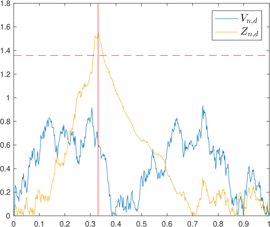
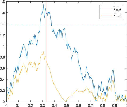
Figure 1. Paths of $|Z_{n,d}(t)|$ and $|V_{N,d}(t)|$ with $w(t)\equiv 1$, $p=1$ based on a single change at $k_{1}=\lfloor N/3\rfloor$ (vertical line) for independent Gaussian observations, $N=d=500$; horizontal dashed line is associated critical value at size $0.05$. In the left figure there is only shift in the mean; on the right, only a change in scale. Jointly maximizing $Z_{N,d}$ and $V_{N,d}$ leads to increased power against a broader array of alternatives in high dimensions.

Though tests based on either $Z_{N,d}$ or $V_{N,d}$ alone are suitable themselves, use of both $Z_{N,d}$ and $V_{N,d}$ together allows for increased power against a broader array of alternatives; see Figure 1. Each is suitable for detecting changes of various types, but $V_{N,d}$ is especially sensitive to scale changes, whereas $Z_{N,d}$ is more sensitive to location changes, and both take into account information concerning $p$-th moments in different capacities. Combining them by jointly maximizing them leads to a testing approach and estimation procedure that are sensitive to a larger variety of distributional changes in high-dimensional contexts. (Note $T_{N,d}$ can be interpreted a test statistic based on a union-intersection test (Roy, 1953) formed from two tests: one based on $V_{N,d}$ and one based on $T_{N,d}$.) In contrast, both $Z_{N,d}$ and $V_{N,d}$ behave somewhat similarly under $H_{0}$, and owing to this, the statistic $T_{N,d}$ in fact enjoys standard limit behavior in high dimensions under $H_{0}$, leading to a straightforward asymptotic test.

The use of the parameter $\beta$ and weight functions $w(t)$ also allows for increased power against certain alternatives regarding type or location of change point(s). Very roughly speaking, the parameter $\beta$ can be viewed a proxy for the relative importance of alternatives measured by $Z_{N,d}(t)$ compared to those measured by $V_{N,d}(t)$, and the weight function $w(t)$ can be chosen to boost power when change points may be near the boundary of an interval. We further discuss the effect of selection of $w(t)$ and the auxiliary parameter $\beta$ in Section 4.

3. Theoretical results

In the statements that follow, we make use of the integral functional

(3.1) $$I(w,c)=\int_{0}^{1}\frac{1}{t(1-t)}\exp\left(-\frac{cw^{2}(t)}{t(1-t)}\right)dt$$

to determine necessary and sufficient conditions to obtain a finite limit for the weighted supremum functionals of $V_{N,d}(t)$ and $Z_{N,d}(t)$.

3.1. Size

We separately consider two distinct settings concerning possible types of dependence in the coordinates of the $\mathbf{X}_{i}$. We defer discussion of implementation of the tests in practice to Section 3.1.3.

3.1.1. Weak dependence

We first turn to the case of weakly dependent coordinates. For the statements below, we define the functions

(3.2) $$g_{j}(x_{j})=E|X_{1,j}-x_{j}|^{p},\;\;1\leq j\leq d,$$

where $x_{1},\ldots,x_{d}\in\mathbb{R}$.

Assumption 3.1.

For some $\alpha>\max\{p,10-4/p,14-8/p\}$, and some constant $C>0$ independent of $d$ and $N$, we have $\max_{1\leq j\leq d}E|X_{1,j}|^{\alpha}\leq C$,

(3.3) $$E\bigg{|}\sum_{j=1}^{d}\big{[}\left|X_{1,j}-X_{2,j}\right|^{p}-E\left|X_{1,j}-X_{2,j}\right|^{p}\big{]}\bigg{|}^{\alpha}\leq Cd^{\alpha/2},$$

and

(3.4) $$E\bigg{|}\sum_{j=1}^{d}\big{[}g_{j}(X_{1,j})-Eg_{j}(X_{1,j})\big{]}\bigg{|}^{\alpha}\leq Cd^{\alpha/2}.$$

Moreover, the limits

(3.5) $$\mathcal{a}(p)=\lim_{d\to\infty}\frac{1}{d}\sum_{j=1}^{d}Eg_{j}(X_{1,j}),\quad\tau^{2}=\lim_{d\to\infty}\frac{1}{d}E\bigg{(}\sum_{j=1}^{d}[g_{j}(X_{1,j})-Eg_{j}(X_{1,j})]\bigg{)}^{2}$$

exist.

Expressions (3.3) and (3.4) roughly state that the coordinates of $\mathbf{X}_{1}$ and of ${\bf X}_{1}-{\bf X}_{2}$ behave like weakly dependent random variables. In particular, they are satisfied for AR(1)-type coordinates (c.f. Example A.2). In Appendix A, we give explicit examples of settings in which Assumptions 3.1 and 3.2 are satisfied. Note when $g_{1}(X_{1,1}),g_{2}(X_{1,2}),\ldots$ is a wide-sense stationary sequence, $\mathcal{a}(p)$ is its mean and $\tau^{2}$ is its corresponding long-run variance. Furthermore, note the distribution of ${\bf X}_{1}$ depends on $d$ and is also allowed to depend on $N$, so our assumptions allow for triangular arrays of random vectors.

Next we define the limiting variance of $V_{N,d}(t)$ and $Z_{N,d}(t)$ for the case of weakly dependent coordinates. Let

(3.6) $$\sigma^{2}=\left(\frac{2}{p}\mathcal{a}^{-1+1/p}(p)\right)^{2}\tau^{2}.$$

Note $\sigma^{2}$ is well-defined under Assumption 3.1. Since we will normalize with $\sigma^{2}$, it is natural to require

Assumption 3.2.

$\sigma^{2}>0$.

Assumption 3.2 amounts to a high-dimensional non-degeneracy condition. Note that similar assumptions are typically not met in fixed dimensions when the underlying U-statistics are of degenerate type.

Theorems 3.1 and 3.2, stated next, are our main results in the context of Assumption 3.1, which provide the asymptotic distribution under of our test statistics under $H_{0}$ after appropriate rescaling. This lays the foundation for our asymptotic testing procedure.

Theorem 3.1.

Assume that $H_{0}$ holds, and Assumptions 2.1, 3.1 and 3.2 are satisfied. If $I(w,c)<\infty$ in (3.1) is finite for some $c>0$, then as $\min\{N,d\}\to\infty,$

(3.7) $$\sigma^{-1}(Nd)^{1/2}T_{N,d}\stackrel{{\scriptstyle{\mathcal{D}}}}{{\to}}\sup_{0<t<1}\frac{|B(t)|}{w(t)},$$

where $\{B(t),0\leq t\leq 1\}$ is a Brownian bridge.

Theorem 3.1 allows for a variety of possible weight functions $w(t)$; since the limit in (3.7) is finite with probability 1 if and only if $I(w,c)<\infty$ with some $c>0$, the conditions on the weight function for Theorem 3.1 are sharp (see Csörgő and Horváth (1993)), as no other classes of weight functions can lead to such a limit.

However, it is sometimes desirable to self-normalize maximally selected statistics, i.e., to use a weight function that is proportional to the standard deviation of the limit, at least in a neighborhood of 0 and 1. In this case, the corresponding weight function is $w(t)=(t(1-t))^{1/2}$, but Theorem 3.1 cannot be applied since $I((t(1-t))^{1/2},c)=\infty$ for all $c>0$. Thus, Theorem 3.2, stated next, can be regarded as a counterpart to Theorem 3.1 for the choice of weight function $w(t)=(t(1-t))^{1/2}$. It is a nonstandard Darling–Erdős–type result, showing Gumbel-type limit behavior emerges under the choice $w(t)=(t(1-t))^{1/2}$.

Before giving its statement, we define some auxiliary quantities based on the projections of U-statistics (e.g., Lee (1990)). For ${\bf x}=(x_{1},x_{2},\ldots,x_{d})$, let

(3.8) $$H({\bf x})=E\left(\frac{1}{d}\sum_{\ell=1}^{d}|X_{1,\ell}-x_{\ell}|^{p}\right)^{1/p},\quad\theta=E[H({\bf X}_{1})].$$

and

(3.9) $$\zeta_{i}=H({\bf X}_{i})-\theta,\;\;\;1\leq i\leq N;\quad\mathcal{s}^{2}(d)=E\zeta_{1}^{2}.$$

i.e., $\zeta_{i}$ are centered projections of the normalized $L_{p}$ norms of the differences $\mathbf{X}_{i}-\mathbf{X}_{j}$ onto the linear space of all measurable functions of $\mathbf{X}_{i}$.

Theorem 3.2.

Define the quantities

(3.10) $$a(x)=(2\log x)^{1/2}\quad\mbox{and}\quad b(x)=2\log x+\tfrac{1}{2}\log\log x-\tfrac{1}{2}\log\pi.$$

If $H_{0}$ holds, and Assumptions 2.1, 3.1, and 3.2 are satisfied, then with $\mathcal{s}(d)$ as in (3.9) and the choice $w(t)=(t(1-t))^{1/2}$, as $\min\{N,d\}\to\infty$,

(3.11) $$P\biggl{\{}\frac{a(\log N)N^{1/2}}{2\mathcal{s}(d)}~{}\!T_{N,d}\leq x+b(\log N)\biggl{\}}\to\exp\left(-2e^{-x}\right)$$

for all $x$. Furthermore,

(3.12) $$\mathcal{s}^{2}(d)=\frac{\sigma^{2}}{4d}+o\left(\frac{1}{d}\right),\;\;\;\;d\to\infty.$$

Theorems 3.1 and 3.2 together provide the high-dimensional theoretical foundation for asymptotic tests based on $T_{N,d}$, encompassing essentially all possible weight functions of practical interest under the weak-type dependence context of Assumption 3.1. Upon selection of $w(t)$, an asymptotic size $\alpha$ test can be conducted simply by rejecting $H_{0}$ if $T_{N,d}$ exceeds the $1-\alpha$ quantile of the corresponding limit, provided a consistent estimate of $\sigma$ is available (on estimating $\sigma$, see Section 3.1.3.)

Remark 3.1.

The processes $V_{N,d},Z_{N,d}$ underlying $T_{N,d}$ are clearly highly dependent since they are both computed from the same sequence of data. Under $H_{0}$, our proofs reveal the joint weak convergence of the $\mathbb{R}^{2}$-valued process $\sigma^{-1}(Nd)^{1/2}\big{(}V_{N,d}(t),Z_{N,d}(t)\big{)}^{\top}$ in the space ${\mathcal{D}}[0,1]$ of $\mathbb{R}^{2}$-valued càdlàg functions on [0,1] to the process

$$\big{(}B(t),(1-2t)^{1-\beta}B(t)\big{)}^{\top},\quad 0\leq t\leq 1,$$

where $B(t)$ is a standard Brownian bridge, which ultimately drives the asymptotic behavior of $T_{N,d}$ under $H_{0}$.

In the next section, we demonstrate the test can also be used under certain types of strong coordinate dependence as well.

3.1.2. Strong dependence.

Next we consider the setting when the coordinates are potentially strongly dependent, in the sense that they are discretely sampled observations of random functions $Y_{i}=\{Y_{i}(t),0\leq t\leq 1\}$, $i=1,\ldots,N$, i.e.,

$${\bf X}_{i}=(Y_{i}(t_{1}),Y_{i}(t_{2}),\ldots,Y_{i}(t_{d}))\;\;\mbox{with some }\;0<t_{1}<t_{2}<\ldots<t_{d}\leq 1.$$

Below is our main assumption in this setting.

Assumption 3.3.

(i) $Y_{1},\ldots,Y_{N}$ are independent and identically distributed and have continuous sample paths with probability 1,
(ii) $d\max_{1\leq i\leq d}(t_{i}-t_{i-1})\to 1,$ $t_{0}=0,t_{d}=1$
(iii)  $E\int_{0}^{1}|Y_{1}(t)|^{r}dt<\infty$ for some $r\geq\max\{4,p\}$,
(iv)  and with some $\nu>2$

$$E\left|\frac{1}{d}\sum_{j=1}^{d}|X_{1,j}|^{p}-\int_{0}^{1}|Y_{1}(t)|^{p}dt\right|^{\nu}\to 0.$$

The projections $H(\mathbf{x})$ in (3.9) can also be approximated with functionals of $Y_{i}(t)$. For any measurable function $g$, we define

$$\mathcal{H}(g)=E\left(\int_{0}^{1}\left|Y_{1}(t)-g(t)\right|^{p}dt\right)^{1/p}$$

whenever the expectation exists and is finite. Next we define the asymptotic variance in the context of strongly dependent coordinates. Let

$$\gamma^{2}=\mbox{\rm var}\left(\mathcal{H}(Y_{1})\right).$$

Note $\gamma^{2}<\infty$ under Assumption 3.3(iii). Since we normalize with $\gamma^{2}$, we naturally require

Assumption 3.4.

$\gamma^{2}>0.$

Theorems 3.3 and 3.4, stated next, are our main results in the context of Assumption 3.3.

Theorem 3.3.

Assume that $H_{0}$ holds and Assumptions 3.3 and 3.4 are satisfied. If $I(w,c)<\infty$ is finite for some $c>0$, then

(3.13) $$\gamma^{-1}N^{1/2}T_{N,d}\stackrel{{\scriptstyle{\mathcal{D}}}}{{\to}}\sup_{0<t<1}\frac{|B(t)|}{w(t)}$$

The next statement is based on the choice of weight function $w(t)=(t(1-t))^{1/2}$ and is the analog of Theorem 3.2 in our strong dependence framework.

Theorem 3.4.

If $H_{0}$ holds and Assumptions 3.3 and 3.4 are satisfied, then with ${\mathcal{s}}(d)$ as in (3.9) and the choice $w(t)=(t(1-t))^{1/2}$, as $\min\{N,d\}\to\infty$,

(3.14) $$P\biggl{\{}\frac{a(\log N)N^{1/2}}{2\mathcal{s}(d)}~{}\!T_{N,d}\leq x+b(\log N)\biggl{\}}=\exp\left(-2e^{-x}\right)$$

for all $x$. Furthermore, ${\mathcal{s}}^{2}(d)=\gamma^{2}/4+o(1)$.

Theorems 3.1 through 3.4 together illustrate our approach is suitable in a variety of distributional settings concerning the dependence of the coordinates. Though the scaling factor for $T_{N,d}$ in Theorems 3.1 and 3.2 is different than in Theorems 3.3 and 3.4 by a factor of $d^{1/2}$, conveniently, in practice the same implementation can be used in either case, as we discuss in the next section.

3.1.3. On implementation

Implementation of asymptotic tests based on Theorems 3.1–3.4 first requires consistent estimation of the asymptotic variances $\sigma^{2}$ and $\gamma^{2}$ and suitable normalization of the test statistics. Below we describe one such approach commonly used for $U$-statistics via the jackknife (e.g., Lee (1990)).

In what follows, let $U_{N,d}$ denote $d^{-1/p}U_{N,d,1}(N)$, and let $U_{N-1,d}^{(-i)}$ denote the value analogous to $U_{N,d}$ but based on the values ${\bf X}_{1},\ldots,{\bf X}_{i-1},{\bf X}_{i+1},\ldots,{\bf X}_{N}$; i.e. ${\bf X}_{i}$ is left out. Define the so-called pseudo-observations

$$\mathcal{U}_{i}=NU_{N,d}-(N-1)U_{N-1,d}^{(-i)}$$

and their corresponding average

$$\bar{\mathcal{U}}_{N}=\frac{1}{N}\sum_{i=1}^{N}\mathcal{U}_{i}.$$

The jackknife estimator for the variance is defined as

$$\hat{\sigma}_{N,d}^{2}=\frac{1}{(N-1)}\sum_{i=1}^{N}(\mathcal{U}_{i}-\bar{\mathcal{U}}_{N})^{2}.$$

The next statement shows that the same test statistic may be used in practice irrespective of which set of assumptions among Sections 3.1.1 and 3.1.2 hold.

Proposition 3.1.

Under either the conditions of Theorem 3.1 or of Theorem 3.3, as $\min\{N,d\}\to\infty$,

$$\frac{N^{1/2}}{\hat{\sigma}_{N,d}}T_{N,d}\stackrel{{\scriptstyle{\mathcal{D}}}}{{\to}}\sup_{0<t<1}\frac{|B(t)|}{w(t)}.$$

To replace the normalizations in the Darling–Erdős–type results of Theorems 3.2 and 3.4, we need an assumption on the rate of convergence of $\widehat{\sigma}^{2}_{N,d}$.

Proposition 3.2.

Under the conditions of Theorem 3.2, if

$$d^{1/2}\left|\hat{\sigma}_{N,d}-2d^{1/2}\mathcal{s}(d)\right|\log\log N\stackrel{{\scriptstyle P}}{{\to}}0$$

Then,

(3.15) $$P\biggl{\{}\frac{a(\log N)N^{1/2}}{\hat{\sigma}_{N,d}}~{}\!T_{N,d}\leq x+b(\log N)\biggl{\}}\to\exp\left(-2e^{-x}\right)$$

for all $x$. Under the conditions of Theorem 3.4, the limit (3.15) holds for all $x$ if

$$\left|\hat{\sigma}_{N,d}-\mathcal{s}(d)\right|\log\log N\stackrel{{\scriptstyle P}}{{\to}}0.$$

Thus, upon choosing the weight function $w(t)$, one can appropriately normalize $T_{N,d}$ using $\hat{\sigma}_{N,d}$ to obtain the same limit distribution under $H_{0}$ in either the weak- or strong- coordinate dependence case. This leads to a testing procedure that, with regards to its asymptotic size, remains indifferent conercerning which assumption among these two sets holds.

Critical values of the limiting test statistics in Theorem 3.1 and Theorem 3.3 may be obtained through various means. For instance, Franke et al. (2022) provide a fast adaptive method to approximate the critical values for the supremum of the Brownian bridge with weight function $w(t)=(t(1-t))^{\kappa}$, $0\leq\kappa<1/2$. Selected critical values for the weighted Brownian bridge are also tabulated in Olmo and Pouliot (2011). If desired, resampling methods can also be used to provide critical values; for instance, one can use the bootstrap as in Gombay and Horváth (1999) and Hušková and Kirch (2008); permutation-based methods can be also used to obtain critical values (cf. Antoch and Hušková (2001)), though at potentially at a substantial computational cost. This is discussed toward the end of Section 4.3.

3.2. Power.

Next we briefly discuss the behavior of the statistics under $H_{A}$. For simplicity we first consider the case of a single change point $(R=1)$ at location $k_{1}$. Power in both single and multiple change scenarios is examined numerically in Section 4.

The next result provides sufficient conditions for high-dimensional consistency of the asymptotic tests given in Section 3.1. For the statements ahead, define

(3.16) $$\mu_{1}=E\|{\bf X}_{1}-{\bf X}_{2}\|_{p},\quad\mu_{2}=E\|{\bf X}_{k_{1}+1}-{\bf X}_{k_{1}+2}\|_{p}$$

and

(3.17) $$\mu_{1,2}=E\|{\bf X}_{1}-{\bf X}_{k_{1}+1}\|_{p}.$$

(N.b.: $\mu_{1},\mu_{2},$ and $\mu_{1,2}$ depend on $d$ and are allowed to depend on $N$.) Also, set

(3.18) $$\widetilde{T}_{N,d}=\begin{cases}\displaystyle\frac{N^{1/2}T_{N,d}}{\mathcal{s}(d)}&\text{if $I(w,c)<\infty$ for some $c$,}\\ \displaystyle\frac{a(\log N)N^{1/2}}{\mathcal{s}(d)}~{}\!T_{N,d}-b(\log N)&w(t)=(t(1-t))^{1/2}.\end{cases}$$

Note that divergence of $\widetilde{T}_{N,d}$ implies the consistency of the associated test in Theorems 3.1–3.4. We also denote $0<\eta<1$ as the break fraction, i.e., the change point $k_{1}$ is given as $k_{1}=\lfloor N\eta\rfloor$.

Theorem 3.5.

Suppose $R=1$ and $k_{1}=\lfloor N\eta\rfloor,$ for some fixed $0<\eta<1$. Let

$$\Delta_{N,d}=d^{-1/p}\max\{|\mu_{1}-\mu_{2}|,|\mu_{1}-\mu_{1,2}|,|\mu_{2}-\mu_{1,2}|\}$$

Then, we have

(3.19) $$\widetilde{T}_{N,d}\stackrel{{\scriptstyle P}}{{\to}}\infty$$

whenever Assumptions 2.1, 3.1 and 3.2 hold, and

1. $(Nd)^{1/2}\Delta_{N,d}\to\infty$, if $w$ is chosen such that $I(w,c)<\infty$ for some $c$,

2. $(Nd)^{1/2}\left(\log\log N\right)^{-1/2}\Delta_{N,d}\to\infty$, if $w(t)=(t(1-t))^{1/2}$.

Under Assumptions 3.3–3.4, (3.19) holds whenever

1. $N^{1/2}\Delta_{N,d}\to\infty$, if $w$ is chosen such that $I(w,c)<\infty$ for some $c$,

2. $N^{1/2}\left(\log\log N\right)^{-1/2}\Delta_{N,d}\to\infty$, if $w(t)=(t(1-t))^{1/2}$.

Observe that the hypotheses of Theorem 3.5 require a stronger separation condition in the context of Assumptions 3.3–3.4 compared to the context of Assumptions 3.1–3.2. For instance, when $\Delta_{N,d}$ is held fixed, the conditions in $(i)$ and $(ii)$ suggest larger values of $d$ lead to improved test power under Assumptions 3.1–3.2, whereas this is not the case for conditions $(i^{\prime})$ and $(ii^{\prime})$ under Assumptions 3.3–3.4. This can roughly be seen as a reflection of the fact that a stronger signal is needed to overcome comparatively stronger coordinate-wise dependence.

It is also worth noting that even if the distributions change at location $k_{1}$, it is still possible that $\mu_{1}=\mu_{2}$ holds. For example, under a location shift, $\mu_{1}=\mu_{2}$, but $\mu_{1}\neq\mu_{1,2}$. Therefore, Theorem 3.5 demonstrates our tests are consistent against a variety of alternatives, encompassing changes in location, scale, and in higher moments.

Though our main focus is testing, the behavior of our test statistics under the alternative can be used to estimate the change point location. Below we provide one such possibility that is consistent under mild additional conditions. Let

$$Z_{N,d,0}(t)=t(1-t)d^{-1/p}\left[U_{N,d,3}(\lfloor Nt\rfloor)-U_{N,d,4}\right],$$

and let

$$k_{V}=\operatorname*{argmax}_{2<k<N-2}\big{|}V_{N,d}\big{(}\tfrac{k}{N}\big{)}\big{|},\quad k_{Z}=\operatorname*{argmax}_{2<k<N-2}\big{|}Z_{N,d,0}\big{(}\tfrac{k}{N}\big{)}\big{|},$$

where the selection of $k_{V},k_{Z}$ is arbitrary among the respective maximizers in the case of ties. Set $t_{V}=k_{V}/N$ and $t_{Z}=k_{Z}/N$. Our estimator is then defined as

(3.20) $$\widehat{\eta}_{N,d}=\begin{cases}t_{V},&|V_{N,d}(t_{V})|\geq|Z_{N,d}(t_{Z})|,\\ t_{Z},&|V_{N,d}(t_{V})|<|Z_{N,d}(t_{Z})|.\end{cases}$$

The idea behind the estimator is as follows. Though the behavior of $Z_{N,d}$ and $V_{N,d}$ is quite similar under $H_{0}$, depending on the type of alternative, their paths under $H_{A}$ can be dramatically different. Selecting the maximizers $t_{Z}$ and $t_{V}$ of the unweighted $Z_{N,d,0}$ and $V_{N,d}$ is done at the first step so that $\beta$ does not influence the location of the estimated change. Then, the change point location is chosen among these candidate locations based on the associated value of the original processes $Z_{N,d}$ and $V_{N,d}$. (Note that, in principle, both $Z_{N,d}$ and $V_{N,d}$ may exceed the critical value: in these cases, the break location is simply selected as the larger among the two.)

The following theorem establishes the consistency of $\widehat{\eta}_{N,d}$.

Proposition 3.3.

Under the hypotheses of Theorem 3.5, for $\widehat{\eta}$ as in (3.20), we have

(3.21) $$\hat{\eta}_{N,d}\stackrel{{\scriptstyle P}}{{\to}}\eta$$

in the setting of Assumptions 2.1, 3.1 and 3.2 whenever

1. $\mu_{1,2}\gg\max\{\mu_{1},\mu_{2},d^{1/p-1/2}N^{-1/2}\}$,

2. $|\mu_{1}-\mu_{2}|\gg\max\{|\mu_{1,2}-\mu_{1}|,|\mu_{1,2}-\mu_{2}|\}\gg d^{1/p-1/2}N^{-1/2}$.

In the setting of Assumptions 3.2-3.3, (3.21) holds whenever

1. $\mu_{1,2}\gg\max\{\mu_{1},\mu_{2},d^{1/p}N^{-1/2}\}$,

2. $|\mu_{1}-\mu_{2}|\gg\max\{|\mu_{1,2}-\mu_{1}|,|\mu_{1,2}-\mu_{2}|\}\gg d^{1/p}N^{-1/2}$.

The conditions for consistency in Proposition 3.3 reflect two qualitatively different types of possible changes: the divergence $(i)$ (and $(i^{\prime})$) can occur due to a location shift, and the divergence $(ii)$ (and $(ii^{\prime})$) can result from scale changes, among other possibilities (in particular, the divergence in $(ii)$ cannot occur due to a location shift).

Remark 3.2.

Upon rejection of $H_{0}$, since $V_{N,d}$ is invariant under location shifts, it may be desirable to know which among $V_{N,d}$ and $Z_{N,d}$ contributed to rejection of $H_{0}$. By virtue of the joint maximization of these statistics through $T_{N,d}$, one can check which among $\sup_{0<t<1}|V_{N,d}(t)|/w(t)$ and $\sup_{0<t<1}|Z_{N,d}(t)|/w(t)$ has exceeded the critical value of the test without increasing the overall type I error rate.

The estimation and testing procedure above can be extended naturally and readily to estimate multiple changes via recursive procedures such as binary segmentation, which we illustrate in Section 4. Though in principle our estimation procedure can potentially be improved further via wild binary segmentation (Fryzlewicz, 2014) or possibly through customized methods that make separate use of $Z_{N,d}$ and $V_{N,d}$, for the sake of illustration and simplicity we focus on the case of ordinary binary segmentation in our numerical study.

4. Simulation study

To evaluate the numerical performance of our procedure, we examine its behavior in simulations based on the choice of the weight function

(4.1) $$w(u)=\frac{1}{(u(1-u))^{\kappa}}\quad\;\;0\leq\kappa\leq 1/2,$$

for various values of $\kappa$. In all settings, unless otherwise stated, we use $\beta=0.9$. Each reported estimate is based on 2000 independent realizations. The asymptotic variance estimates used in each case are based on the jackknife method described in Section 3.1.3.

4.1. Size

We examine empirical size of our test at the sample sizes $N=50,100,250,500$ with $d=N$ and $d=2N$ where $\mathbf{X}_{i}$ are independent copies of $\mathbf{X}=(X_{1},\ldots,X_{n})$, in the following settings:

1. $\mathbf{X}\sim N(0,\mathbf{I}_{d})$;

2. AR(1) coordinates: $X_{i}=\phi X_{i-1}+\varepsilon_{i}$, with $\phi=0.9$ and $\varepsilon_{i}\stackrel{{\scriptstyle iid}}{{\sim}}N(0,1)$.

3. $\mathbf{X}\sim\text{Multinomial}(5d,\mathbf{p})$, with $\mathbf{p}=(p_{1},\ldots,p_{d})$, where $p_{i}=(1/i)\big{(}\sum_{j=1}^{d}1/j\big{)}^{-1}$.

For brevity we display results only for $p=1$, though other cases of $p=2,3$ performed similarly in our simulations. Below are tables for nominal sizes $0.01$ and $0.05$.

Nominal size $0.01$
		$N=d$				$N=d/2$
	$\kappa$	50	100	250	500	50	100	250	500
Ex $(1)$	0	.007	.008	.008	.010	.004	.006	.006	.007
	.2	.005	.005	.009	.009	.005	.007	.011	.008
	.4	.013	.010	.007	.011	.015	.010	.009	.012
	.45	.024	.020	.021	.017	.017	.019	.016	.011
Ex (2)	0	.003	.003	.007	.010	.005	.010	.006	.007
	.2	.004	.005	.009	.006	.004	.009	.011	.008
	.4	.016	.011	.010	.009	.014	.009	.012	.009
	.45	.014	.017	.017	.015	.023	.029	.022	.020
Ex (3)	0	.007	.007	.009	.008	.004	.005	.005	.006
	.2	.006	.006	.008	.007	.006	.010	.0075	.006
	.4	.025	.014	.011	.012	.024	.019	.011	.010
	.45	.030	.027	.010	.016	.034	.017	.018	.016

Nominal size $0.05$
		$N=d$				$N=d/2$
	$\kappa$	50	100	250	500	50	100	250	500
Ex $(1)$	0	.026	.032	.039	.048	.028	.038	.047	.046
	.2	.036	.044	.040	.042	.037	.034	.043	.044
	.4	.064	.054	.044	.051	.053	.058	.050	.044
	.45	.065	.069	.064	.053	.061	.069	.079	.069
Ex (2)	0	.027	.033	.036	.043	.023	.035	.042	.036
	.2	.037	.033	.039	.045	.030	.040	.050	.049
	.4	.060	.058	.049	.047	.060	.063	.047	.042
	.45	.059	.067	.061	.06	.064	.071	.070	.062
Ex (3)	0	.034	.033	.039	.041	.024	.034	.036	.033
	.2	.044	.038	.049	.046	.029	.034	.035	.047
	.4	.070	.059	.058	.052	.069	.058	.058	.059
	.45	.072	.067	.061	.069	.064	.064	.066	.064

Table 1. Empirical size for nominal size $\alpha=0.01$ and $\alpha=0.05$ tests with $p=1$ in Examples $(1)$–$(3)$.

In general, the test tends to be more aggressive as $\kappa$ increases, particularly in the case of $\kappa=0.45$ when it is consistently oversized. (Since the convergence rate for $\kappa=0.5$ is particularly slow, we do not recommend use of $\kappa=0.5$ at this sample size.) Generally the size approximation is closest to the nominal value for the case $\kappa=0.2$ and $\kappa=0.4$ for values of $N\geq 100$. There is little difference between the settings with $d=2N$ and $d=N$, or between examples (1)–(3).

4.2. Power.

We study power and estimation performance in a variety of settings. For comparison against other methods suited for general changes, we compare our method with

• (E-div.): the nonparametric E–divisive method (Matteson and James, 2014) via the ecp package in R. This method involves choice of a parameter $\alpha\in(0,2)$; in our simulations we consider ordinary energy distance ($\alpha=1$). Unless otherwise indicated we use default settings for the e.divisive() method.

• (MEC): The graph-based max-type edge count method (Chu and Chen (2019)) via the gSeg package in R. This method is suitable for a variety of datatypes and is demonstrated in their work to have some advantages in high dimensions. Following their simulation examples, we apply their method using the $k$-minimum-spanning tree graph based on Euclidean distances with $k=5$.

In all of our simulations in this section, we consider tests at the 5% significance level.

4.2.1. Single change setting.

We first examine the effect of the various types of distributional changes for a single change point in high dimensions with $N=d$ at location $\lfloor k_{1}/N\rfloor=\eta\in\{0.5,0.75\}$. In what follows, we let $\mathbf{Y}(\phi)=(Y_{1},\ldots,Y_{d})^{\top}$ denote vector of AR(1) coordinates, where $Y_{i}=\phi Y_{i-1}+\varepsilon_{i}$ and $\varepsilon_{i}\stackrel{{\scriptstyle iid}}{{\sim}}N(0,1)$. Also, below, $t(\nu)$ denotes a Students’ $t$ random variable with $\nu$ degrees of freedom. For the single change-point setting, we consider:

1. Location change: $\mathbf{X}_{1}\stackrel{{\scriptstyle d}}{{=}}\mathbf{Y}(\phi)$ and $\mathbf{X}_{k_{1}+1}\stackrel{{\scriptstyle d}}{{=}}\mathbf{Y}(\phi)+\boldsymbol{\mu}$, with $\phi=0.5$, $\boldsymbol{\mu}=(0.2,\ldots,0.2)^{\top}$

2. Covariance change: $\mathbf{X}_{1}\stackrel{{\scriptstyle d}}{{=}}\mathbf{Y}(\phi)$, and $\mathbf{X}_{k_{1}+1}\stackrel{{\scriptstyle d}}{{=}}\mathbf{Y}(\phi^{\prime})$, with $\phi=0.5$, $\phi^{\prime}=0.55$. (Note this amounts to a roughly 7.5% gain in variance in addition to correlation changes.)

3. Tail change: $\mathbf{X}_{1}\sim N(0,\mathbf{I}_{d})$, and $\mathbf{X}_{k_{1}+1}=(X_{k_{1}+1,1},\ldots X_{k_{1}+1,d})$ with $X_{k_{1}+1,i}\stackrel{{\scriptstyle iid}}{{\sim}}t(\nu)/\sqrt{\operatorname{var}(t(\nu))}$, where $\nu=7$. (Note the first three moments remain constant throughout.)

For E-div, when $N\leq 100$, we set the minimum cluster size to 10; otherwise we leave it as its default value (30). For MEC, we use the function gSeg1(), as is recommended in the package documentation (Chen et al. (2021)) for the single change-point setting.

		$\eta=0.5$					$\eta=0.75$
	$N=d$	$p=1$	$p=2$	$p=3$	E-div.	MEC	$p=1$	$p=2$	$p=3$	E-div.	MEC
Ex (4)	50	.059	.045	.055	.210	.135	.057	.052	.049	.113	.117
	100	.094	.071	.093	.620	.277	.057	.049	.053	.381	.201
	150	.455	.446	.442	.985	.553	.058	.054	.065	.901	.376
	200	.937	.938	.923	.999	.826	.076	.075	.068	.998	.599
	250	1.00	1.00	.998	.991	.996	.114	.101	.112	1.00	.817
Ex (5)	50	.090	.092	.087	.045	.073	.092	.078	.078	.052	.076
	100	.274	.291	.268	.069	.085	.228	.197	.213	.052	.069
	150	.598	.617	.605	.043	.112	.492	.452	.478	.040	.110
	200	.884	.878	.878	.048	.141	.755	.760	.742	.041	.120
	250	.984	.982	.984	.042	.207	.907	.927	.925	.053	.203
Ex (6)	50	.087	.041	.064	.041	.208	.075	.067	.094	.048	.186
	100	.258	.060	.144	.035	.300	.227	.071	.204	.052	.337
	150	.561	.060	.347	.042	.396	.445	.070	.373	.057	.365
	200	.847	.055	.624	.041	.454	.720	.083	.625	.048	.426
	250	.971	.066	.864	.045	.392	.910	.092	.812	.037	.467

Table 2. Power in the single change-point settings of Examples $(4)$–$(6)$ at the changepoint locations $\eta=0.5$ and $\eta=0.75$. $T_{N,d}$ is calculated based on $\beta=0.9$ and $w(t)$ as in (4.1) with $\kappa=0.4$. We consider $p=1,2,3$ in (2.1) (corresponding to three leftmost columns in each group). Boldface numbers indicate the method with the highest power in each row.

In general we see that E-div performs extremely well under a mean change as in setting (4), though MEC and our method still have reasonably good power by comparison for $N=d=200$ and larger when $\eta=0.5$. Rather surprisingly, both E-div and MEC are severely underpowered in setting (5), and our method substantially outperforms both comparison methods in high dimensions. In setting (6), the MEC method has good power for smaller $d$, but ultimately in high dimensions our method outperforms both MEC and E-div, provided $p\neq 2$. Note that in (6), both the E-div method and our approach with $p=2$ have severe lack of power, in agreement with the phenomenon concerning limitations of Euclidean energy distance-related metrics pointed out in Chakraborty and Zhang (2021b). Since our method with $p=2$ is roughly similar to the Euclidean energy distance, this is somewhat expected.

In general our method has its highest power when $\eta=0.5$, as is expected and is common in most change-point methods. When $\eta=0.75$, at this sample size our approach displays a drop in power for mean changes compared to Ediv and MEC, but retains reasonably good power for settings (6) and (7). Though power certainly expected to decrease further in these settings as $\eta$ moves toward the boundary, this is partly compensated by the choice of weight function $w(t)$ with $\kappa=0.4$. This likely can be further mitigated by increasing $\kappa$, though potentially at the expense of some control over size in moderately sized samples.

4.2.2. Multiple change setting.

In practice, the number of change points $R$ and their locations are unknown. For illustration, below we examine the effect of multiple changes in settings with a random number $\mathcal{R}\sim 1+\text{Poisson(1)}$ of change points at locations $\eta_{i}=\lfloor k_{i}/N\rfloor=i/(R+1)$. For simplicity of exposition, we consider “switching” scenarios that alternate between two distributional behaviors analogous to Examples (4)–(6). Specifically, for every integer $j$ with $0\leq 2j\leq\mathcal{R}$, recalling $k_{0}=1$, $k_{R}=N$, we consider

1. Location change: $\mathbf{X}_{k_{2j}}\stackrel{{\scriptstyle d}}{{=}}\mathbf{Y}(\phi)$, and if $2j<\mathcal{R}$, $\mathbf{X}_{k_{2j}+1}\stackrel{{\scriptstyle d}}{{=}}\mathbf{Y}(\phi)+\mu$, with $\phi=0.5$, $\boldsymbol{\mu}=(0.2,\ldots,0.2)^{\top}$,

2. Covariance change: $\mathbf{X}_{k_{2j}}\stackrel{{\scriptstyle d}}{{=}}\mathbf{Y}(\phi)$, and if $2j<\mathcal{R}$, $\mathbf{X}_{k_{2j}+1}\stackrel{{\scriptstyle d}}{{=}}\mathbf{Y}(\phi^{\prime})$, with $\phi=0.5$, $\phi^{\prime}=0.55$.

3. Tail change: $\mathbf{X}_{k_{2j}}\sim N(0,\mathbf{I}_{d})$, and if $2j<\mathcal{R}$, $\mathbf{X}_{k_{2j}+1}=(X_{k_{2j}+1,1},\ldots X_{k_{2j}+1,d})$ with $X_{k_{2j}+1,i}\stackrel{{\scriptstyle iid}}{{\sim}}t(\nu)/\sqrt{\operatorname{var}(t(\nu))}$, $\nu=7$. (As in Example (6), the first three moments remain constant throughout.)

In scenarios $(7)$–$(9)$, each replication has its own independent realization of $\mathcal{R}\in\{1,2,\ldots\}$. In our simulations, we estimate the unknown number of change points $\mathcal{R}$ and change point locations recursively at the 5% level of significance using ordinary binary segmentation. To assess estimation performance of both the estimated number of changes $\widehat{\mathcal{R}}$ and the estimated change point locations in high dimensions, in the table below, we we consider the high dimensional setting of $N=d$, with $N=300,400,500,600$, and report

• The mean and median of the error $\widehat{\mathcal{R}}-\mathcal{R}$

• The average Rand index (RI) and average adjusted Rand index (ARI).

The RI and ARI are measures of agreement between two clusterings of data. In each realization, we compute the RI and ARI based on the estimated partition dictated by the estimated change point location(s) compared with the true partition for that realization consisting of $\mathcal{R}+1$ clusters. Values near 1 indicate strong agreement with the clusterings, i.e., between the estimated number of change points and their true values, in addition to estimated change point locations and their true values. Values near 0 indicate strong disagreement. For more details on the Rand and adjusted Rand indices, we refer to Rand (1971) and Morey and Agresti (1984).

		$T_{N,d}$,    Bin. Seg.				E-div.				MEC, Bin. Seg.
		$\widehat{\mathcal{R}}-\mathcal{R}$		Rand idx.		$\widehat{\mathcal{R}}-\mathcal{R}$		Rand idx.		$\widehat{\mathcal{R}}-\mathcal{R}$		Rand idx.
	$N=d$	$Q_{2}$	Mean	RI	ARI	$Q_{2}$	Mean	RI	ARI	$Q_{2}$	Mean	RI	ARI
Ex (7)	300	-2	-1.54	.524	.311	0	0.04	.985	.967	-2	-1.27	.610	.425
	400	-2	-1.50	.559	.369	0	0.04	.991	.978	0	-0.99	.684	.524
	500	-2	-1.42	.578	.398	0	0.05	.994	.986	0	-0.99	.684	.524
	600	-2	-1.33	.604	.430	0	0.05	.995	.989	0	-0.26	.847	.758
Ex (8)	300	-2	-0.62	.800	.675	-2	-1.91	.384	.023	-2	-1.51	.499	.233
	400	0	-0.09	.928	.862	-2	-1.89	.390	.025	-2	-1.34	.565	.350
	500	0	0.12	.969	.930	-2	-1.89	.391	.029	0	-0.96	.666	.500
	600	0	0.20	.978	.949	-2	-1.98	.384	.031	0	-0.52	.787	.673
Ex (9)	300	-2	-0.68	.784	.652	-2	-1.98	.377	.021	-2	-1.70	.411	.065
	400	0	-0.16	.918	.845	-2	-1.93	.384	.019	-2	-1.71	.431	.116
	500	0	0.05	.962	.918	-2	-1.90	.389	.019	-2	-1.59	.441	.134
	600	0	0.14	.976	.944	-2	-1.91	.383	.023	-2	-1.53	.471	.180

Table 3. Estimation accuracy with a random $\mathcal{R}\sim 1+\text{Poisson}(1)$ number of change points in the setting of Examples $(7)$–$(9)$. $Q_{2}$ denotes the median of $\widehat{\mathcal{R}}-\mathcal{R}$. $T_{N,d}$ (leftmost group) is calculated based on $\beta=0.9$, $w(t)$ as in (4.1) with $\kappa=0.4$, and in (2.1) we take $p=1$. Boldface numbers indicate the method with the highest average ARI in each row.

For E-div, we use the same settings as in the Section 4.2.1. For MEC, we continue to use the gSeg1() function with the same settings to accommodate the possibility of only one change point in each realization; repeated application of this method is recommended in the gSeg package documentation as an approach for detecting multiple changes. We implement ordinary binary segmentation to facilitate direct comparison with applying binary segmentation to our procedure.

In general our method has good estimation accuracy in settings (8) and (9). We see that in all settings, behavior analogous to the single change-point setting emerges: except for location changes, our method has dramatically higher performance by comparison to Ediv; the same is true in setting (9) compared to MEC, and in setting (8), our method outperforms both approaches, but MEC retains reasonable estimation performance. For the multiple mean-change setting (7), E-div still dominates for these parameter choices, followed by MEC, and by comparison to the single change-point setting, our estimation performance deteriorates though it retains moderate levels of ARI.

4.3. Discussion

Among the three types of changes considered, our test has reasonably good performance across an array of alternatives, and can have high power and good estimation accuracy in high-dimensional settings settings where other nonparametric methods are relatively powerless or have difficulty correctly estimating change points. Though no single method is expected to uniformly perform best against every type of alternative, our procedure still displays moderate power and estimation accuracy in high dimensions even when it is outperformed for location-only alternatives, whereas comparison methods can be severely underpowered for covariance or tail changes, indicating our approach may be a suitable for use when little knowledge about the anticipated change points is to be assumed. In settings in which location changes are of primary interest, however, likely a procedure suited specifically to location changes would be more appropriate.

In addition, though not explored in-depth in this study, there may be possible advantages of increasing $p$. As evident from Table 2, larger values of $p$ appear to lead to a decrease in power for the given alternatives in settings (4)–(6). However, for sparse alternatives in which only a small portion of coordinates change, increasing $p$ may provide some benefit; unreported simulation studies suggest increasing $p$ can help with power against sparse location alternatives, in particular, but less so for sparse covariance or sparse tail changes.

Further, unreported simulation studies suggest in most settings it is best to take $\beta$ close to 1; though control over size can degrade when making it extremely close to 1 (e.g., say 0.99) in moderate $(N\leq 500)$ sample sizes; in general recommend that $\beta\leq 0.9$ when $N\leq 500$, and $\beta\leq 0.5$ for small sample sizes. $\beta$ also influences the balance of the two statistics $V_{N,d}$ and $Z_{N,d}$ underlying our method; for smaller $\beta$, $Z_{N,d}$ is somewhat deprioritized and our test sensitivity is altered in a nontrivial way, partly becoming less sensitive to location alternatives. On the other hand, increasing $\beta$ over larger samples can lead to increases in power against location alternatives. To minimize the choice of tuning parameters in practice, we recommend in general setting $\beta=0.9$ which seems to work reasonably well in a variety of scenarios.

Our procedure can likely improved in a variety of ways without making significant changes to the underlying method. For instance, estimation performance in the multiple change point setting is expected to improve with wild binary segmentation (Fryzlewicz, 2014). Over moderate and smaller-sized samples in particular, power can likely also be improved though refined normalization of $Z_{N,d}(t)$, e.g., replacing $(|1-2t|+N^{-1/2})^{-\beta}$ by $(|1-2t|+h_{N}(t))^{-\beta}$ or similar, for a function $h_{N}(t)$ satisfying $h_{N}(1/2)\sim N^{-1/2}$ but equal to 1 outside a neighborhood of $t=1/2$. Also note in the multiple change setting, in (3.20), each of $t_{V}$ and $t_{Z}$ may concentrate around different change points, but only one of $t_{V}$ and $t_{Z}$ are chosen as the segmentation point, which may result in losses in power in the subsequent iteration of the binary segmention. This could potentially be improved by running parallel segmentations that take into account which statistic(s) exceed the critical value, which in principle would also provide a more detailed analysis of the observed sequence.

Lastly, in small samples, in lieu of using our asymptotic approach, a standard permutation-based test for $T_{N,d}$ can instead be used to retain control over size. However our method as well as E-div have quadratic complexity as the sample size increases, and permutation-based approaches require repeated rearrangements of $O(N^{2})$ distances for each permutation that can be computationally burdensome when $N$ is large (even when a small number of random permutations are chosen, c.f. Biau et al. (2016)). Our asymptotic approach has the benefit of avoiding this problem and makes our test suitable for testing potentially longer sequences compared with resampling approaches.

5. Application: mentions of U.S. governors on Twitter

We illustrate our method through an application involving Twitter data concerning mentions of U.S. governors. The data was collected using the full–archive tweet counts endpoint in the Twitter Developer API. The API allows retrieval of the count by day of tweets matching any query from the complete history of public tweets. Note that when using the full-archive tweet counts endpoint in the Twitter API, the filters -is:retweet -is:reply -is:quote were applied to remove retweets, replies and quote tweets respectively.

Our dataset consists of matching queries that reference any of the 50 U.S. governors from 1/1/21 to 12/31/21, resulting in a series of length and dimension $(N,d)=(365,50)$. Only governors holding office on the date 12/31/21 were included in this dataset; the full list of queried names is given in Table 5.4.

To accommodate variability in the total number of daily mentions among all governors, which range from roughly 1,000 to 20,000 mentions in a given day, a subset of $m=500$ observations on each day were randomly sampled without replacement, resulting in conditionally multivariate hypergeometric observations $\mathbf{X}_{i}$ with parameters $m=500$, $\mathbf{r}_{i}$, where the vector ${\mathbf{r}}_{i}=(r_{1,i},\ldots,r_{50,i})$ contains the observed number of daily mentions for each governor based on the random selection for that day. Test results did not substantially change for other choices of $m\leq 1000$, and repeated tests for different subsets of $m$ gave relatively consistent results.

U.S. Governors holding office on 12/31/21

Greb Abbott, Charlie Baker, Andy Beshear, Kate Brown, Doug Burgum, John Carney, Roy Cooper, Spencer Cox, Ron DeSantis, Mike Dewine, Doug Ducey, Mike Dunleavy, John Bel Edwards, Tony Evers, Greg Gianforte, Mark Gordon, Michelle Grisham, Kathy Hochul, Larry Hogan, Eric Holcomb, Asa Hutchinson, David Ige, Jay Inslee, Kay Ivey, Jim Justice, Laura Kelly, Brian Kemp, Ned Lamont, Bill Lee, Brad Little, Dan McKee, Henry McMaster, Janet Mills, Phil Murphy, Gavin Newsom, Kristi Noem, Ralph Northam, Mike Parson, Jared Polis, J.B. Pritzker, Tate Reeves, Kim Reynolds, Pete Ricketts, Phil Scott, Steve Sisolak, Kevin Stitt, Chris Sununu, Tim Walz, Gretchen Whitmer, Tom Wolf

Table 5.4. Governor names used for query in Twitter data collection

For our tests and estimation, we use $p=1$ and $\beta=0.9$ in accordance with favorable performance of these choices revealed in Section 4. After a change is detected, we estimate the location of change with $\hat{\eta}_{N,d}$, the estimator of (3.20) with weight function $w(t)=(t(1-t))^{\kappa}$ with for various $\kappa$ and continue to estimate changes via binary segmentation and tests were repeated in each subsegment until failure to reject the null hypothesis. Figure 5.1 contains detected change points for $p=1$, which were identical for choices of $\kappa=0.0,0.1,0.2,0.25,0.4$ and $\beta=0.9$ at significance level $0.01$.

Several detected changes apparently coincide with important dates or events in the U.S. news cycle. For instance, the date 9/12/21 (adjacent to 9/11) is detected as a change point, as is the date 11/25/21, coinciding with the weekend following Thanksgiving; some news events are apparent from other dates. For instance, the date 5/21/2021 coincides with several news stories following Texas Governor Greg Abbott’s signing of the controversial Texas Heartbeat Act into law; the date 8/1/2021 coincides with a news cycle immediately following Florida Governor Ron Desantis’ executive order on 7/30/2021 concerning masking. Interestingly, unreported results from repeated analysis on this dataset across various values of $\beta=0,0.1,0.2,0.3,0.4$ and $\kappa=0,0.2,0.4$ reveals the dates 5/21/21, 8/1/21, and 9/12/2021 are all detected in nearly every case.

for tree=grow=south,circle,draw,minimum size=1ex,inner sep=2mm,s sep=3mm, l sep+=-3ex [Nov. 27 [Aug. 1 [ Feb. 2    [,no edge, draw=none][,no edge, draw=none][,no edge, draw=none][,no edge, draw=none][,no edge, draw=none][,no edge, draw=none][,no edge, draw=none][,no edge, draw=none] [ Apr. 6 [,no edge, draw=none][,no edge, draw=none][Mar. 25][,no edge, draw=none][,no edge, draw=none][,no edge, draw=none][May 21 [May 9][,no edge, draw=none][,no edge, draw=none] ][,no edge, draw=none][,no edge, draw=none] ] ][,no edge, draw=none][,no edge, draw=none][,no edge, draw=none][,no edge, draw=none] [ Oct. 15 [ Sep. 12 [Aug 30] [,no edge, draw=none] ] [,no edge, draw=none] ][,no edge, draw=none][,no edge, draw=none][,no edge, draw=none][,no edge, draw=none][,no edge, draw=none] ][,no edge, draw=none][,no edge, draw=none][,no edge, draw=none][,no edge, draw=none][,no edge, draw=none][,no edge, draw=none][,no edge, draw=none][Dec. 15][,no edge, draw=none][,no edge, draw=none][,no edge, draw=none] ]

Figure 5.1. Change-point detection with size $0.01$ tests using $p=1$ for Governor dataset from January 1st, 2021 to December 31st, 2021. Bisection conducted until failure to reject null hypothesis. In the figure above, the top of each tree is the first estimated change point; subsequent estimated change points after bisection appear along each respective branch in the order of detection, displayed chronologically left–to–right.

6. Conclusion

In this paper, we construct an asymptotic testing procedure suitable for high-dimensional settings based on combining two maximally selected statistics stemming from $L_{p}$ norms. Our method is theoretically supported in high dimensional asymptotic settings and displays convenient limit behavior leading to a straightforward asymptotic test with readily available critical values. We have demonstrated our test has reasonably good power against a variety of alternatives, and has especially high power when there is no change in location by comparison to other nonparametric methods, making it suited to scenarios when little a priori knowledge is available about the type of possible change points or when location changes are not expected.

An underlying principle of our approach lies in combining two separate statistics – each measuring different aspects of the data – that behave similarly under $H_{0}$, leading to tractable and convenient limit behavior, but behave differently under $H_{A}$, thereby providing increased power. This general principle can likely be used in other high-dimensional change-point methods, or to develop more discerning change-point tests and estimation procedures. We leave this open as a topic for future research.

Appendix A Some examples

In this section, we provide some examples in which the assumptions in Section 3 are satisfied. Throughout, $C>0$ denotes a generic constant independent of $N,d$ whose value may change line-to-line.

Example A.1 (Independent coordinates).

Assume $X_{1,1},X_{1,2},\ldots,X_{1,d}$ are independent, and that (3.5) holds. For simplicity write ${\bf X}_{1}-{\bf X}_{2}=(Z_{1},Z_{2},\ldots,Z_{d})^{\top}$. Using Rosenthal’s inequality (Petrov, 1995, p. 59) we get for all $\beta\geq 2$

$$E\Bigg{|} \sum_{j=1}^{d}\big{(}|Z_{j}|^{p}-E|Z_{j}|^{p}\big{)}\bigg{|}^{\beta}$$

$$\leq C\Bigg{(}\sum_{j=1}^{d}E\big{|}|Z_{j}|^{p}-E|Z_{j}|^{p}\big{|}^{\beta}+\bigg{[}\sum_{j=1}^{d}\operatorname{var}\big{(}|Z_{j}|^{p}\big{)}\bigg{]}^{\beta/2}\Bigg{)},$$

where $C>0$ depends only on $p$. Similarly,

$$E\bigg{|} \sum_{j=1}^{d}\big{[}g_{j}(X_{1,j})-Eg_{j}(X_{1,j})\big{]}\bigg{|}^{\beta}$$

$$\leq C\Bigg{(}\sum_{j=1}^{d}E\big{|}g_{j}(X_{1,j})-Eg_{j}(X_{1,j})\big{|}^{\beta}+\bigg{[}\sum_{j=1}^{d}\operatorname{var}\big{(}g_{j}(X_{1,j})\big{)}\bigg{]}^{\beta/2}\Bigg{)}.$$

Note for all $\beta\geq 1$, $E|g_{j}(X_{1,j})|^{\beta}\leq CE|X_{1,j}|^{p\beta}$. Hence conditions (3.3) and (3.4) in Assumption 3.1 are satisfied if

$$\limsup_{d\to\infty}\frac{1}{d}\sum_{j=1}^{d}E|X_{1,j}|^{2p}<\infty$$

and

$$\limsup_{d\to\infty}\frac{1}{d^{\alpha/2}}\sum_{j=1}^{d}\left[E|X_{1,j}|^{p\alpha}+(E|X_{1,j}|^{p})^{\alpha}\right]<\infty.$$

Next we extend Example A.1 to dependent coordinates.

Example A.2 (Linear process coordinates).

Suppose for each $d$, $\mathbf{X}_{i}=(X_{i,1},\ldots,X_{i,d})^{\top}$ are given by $X_{i,\ell}=\sum_{j=-\infty}^{\infty}a_{\ell-j}\varepsilon^{(i)}_{j}$, where $\varepsilon^{(i)}_{j}$ are independent identically distributed variables with $E\varepsilon_{j}^{(i)}=0$, $E(\varepsilon_{i}^{(i)})^{2}=1$, $E|\varepsilon_{1}|^{p\alpha}<\infty$, and the coefficients $a_{k}$ satisfy

(A.1) $$|a_{k}|\leq c_{1}\exp(-c_{2}|k|)$$

with some $0<c_{1},c_{2}<\infty$. First we show (3.3) holds, i.e., that

(A.2) $$E\bigg{|}\sum_{j=1}^{d}\left[|Z_{j}|^{p}-E|Z_{j}|^{p}\right]\bigg{|}^{\alpha}\leq Cd^{\alpha/2}$$

where $(Z_{1},Z_{2},\ldots,Z_{d})^{\top}={\bf X}_{1}-{\bf X}_{2}$. For notational simplicity let $\varepsilon_{j}=\varepsilon_{j}^{(1)}-\varepsilon_{j}^{(2)}$, and for $c_{3}>0$, define

$$\bar{Z}_{j}=\sum_{|j-\ell|\leq c_{3}\log d}a_{\ell-j}\varepsilon_{\ell}+\sum_{|j-\ell|>c_{3}\log d}a_{\ell-j}\widetilde{\varepsilon}_{\ell},$$

where the sequence $\{\widetilde{\varepsilon}_{j}\}_{j=-\infty}^{\infty}$ is an independent copy of $\{\varepsilon_{j}\}_{j=-\infty}^{\infty}$. Let $q\geq 1$ be such that $q^{-1}+r^{-1}=1$, and take any $s>\frac{1}{r}$. The decay of $a_{j,k}$ implies we can choose $c_{3}=c_{3}(\alpha)$ large enough so that

$$E|Z_{j}-\bar{Z}_{j}|^{r} =E\bigg{|}\sum_{|j-\ell|>c_{3}\log d}a_{\ell-j}\widetilde{\varepsilon}_{\ell}\Big{|}^{r}$$

$$\leq\bigg{(}\sum_{|j-\ell|>c_{3}\log d}|j-\ell|^{sq}|a_{\ell-j}|^{q}\bigg{)}^{\frac{r}{q}}\bigg{(}\sum_{|j-\ell|>c_{3}\log d}|j-\ell|^{-sr}E|\widetilde{\varepsilon}_{\ell}|^{r}\bigg{)}$$

$$\leq C\bigg{(}\sum_{|j-\ell|>c_{3}\log d}|j-\ell|^{sq}|\exp\{-qc_{2}|j-\ell|\}\bigg{)}^{\frac{r}{q}}$$

$$\leq Cd^{-\alpha/2}.$$

Using the inequality $||x|^{p}-|y|^{p}|\leq C_{p}(|x|^{p-1}+|y|^{p-1})|x-y|$, this gives

(A.3) $$E\bigg{|}\sum_{j=1}^{d}\big{|}Z_{j}|^{p}-|\bar{Z}_{j}\big{|}^{p}\bigg{|}^{\alpha} \leq CE\Bigg{(}\sum_{j=1}^{d}(|Z_{j}|^{p-1}+|\bar{Z}_{j}|^{p-1})|Z_{j}-\bar{Z}_{j}|\Bigg{)}^{\alpha}$$

(A.4) $$\leq Cd^{\alpha-1}\sum_{j=1}^{d}E\Big{(}(|Z_{j}|^{p-1}+|\bar{Z}_{j}|^{p-1})|Z_{j}-\bar{Z}_{j}|\Big{)}^{\alpha}$$

(A.5) $$\leq d^{\alpha-1}C\sum_{j=1}^{d}\big{(}E|Z_{j}|^{p\alpha}\big{)}^{\frac{p-1}{p}}\big{(}E|Z_{j}-\bar{Z}_{j}|^{p\alpha}\big{)}^{1/p}\leq Cd^{\alpha/2}.$$

Thus, it suffices to establish (A.2) for the variables $\bar{Z}_{j}$ in place of $Z_{j}$. Note that by definition, $\bar{Z}_{1},\bar{Z}_{2},\ldots,\bar{Z}_{d}$ are $c_{3}\log d$–dependent random variables. For simplicity, for each $d$ we set $\bar{Z}_{\ell}=0$ whenever $\ell>d$. Now define $n_{k}=(k-1)\lfloor(\log d)^{2}\rfloor$, $\zeta_{j}=|\bar{Z}_{j}|^{p}-E|\bar{Z}_{j}|^{p}$. Let

$$Q_{k,1}=\sum_{\ell=n_{k-1}+1}^{n_{k}}\zeta_{\ell},\;\;\;k=1,3,\ldots,k^{*}_{1},\qquad Q_{k,2}=\sum_{\ell=n_{k-1}+1}^{n_{k}}\zeta_{\ell},\;\;\;k=2,4,\ldots,k^{*}_{2},$$

where $k_{1}^{*},$ and $k_{2}^{*}$ are the smallest odd and even integers, respectively, such that $n_{k_{i}^{*}}\geq d$. (Note the quantities $Q_{k^{*}_{1},1}$ and $Q_{k^{*}_{2},2}$ respectively may contain fewer than $n_{k^{*}_{1}}-n_{k^{*}_{1}-1}$ and $n_{k^{*}_{2}}-n_{k^{*}_{2}-1}$ terms.) By construction, the variables $Q_{k,1},k=1,3,\ldots,k^{*}_{1}$ are independent and similarly $Q_{k,2}$, $k=2,4,\ldots,k^{*}_{2}$ are independent. Thus, using Rosenthal’s inequality again, we obtain

(A.6) $$E\bigg{|}\sum_{k=1,3,\ldots,k^{*}_{1}}Q_{k,1}\bigg{|}^{\alpha}\leq c_{9}\left(\sum_{k=1,3,\ldots,k^{*}_{1}}E|Q_{k,1}|^{\alpha}+\Big{(}\sum_{k=1,3,\ldots,k^{*}_{1}}E(Q_{k,1})^{2}\Big{)}^{\alpha/2}\right)$$

and similarly for $Q_{k,2}$. We proceed to bound $E|Q_{k,1}|^{\alpha}$ and $E|Q_{k,1}|^{2}$ separately. For $E|Q_{k,1}|^{\alpha}$, we have

(A.7) $$E|Q_{k,1}|^{\alpha}\leq(n_{k}-n_{k-1})^{\alpha-1}\sum_{\ell=n_{k-1}+1}^{n_{k}}E|\zeta_{\ell}|^{\alpha}\leq C(n_{k}-n_{k-1})^{\alpha}\leq C(\log d)^{2\alpha}.$$

For $E|Q_{k,1}|^{2}$, we need a sharper bound. For each $j$, set

$$\bar{\varepsilon}_{\ell}^{(j)}=\begin{cases}\varepsilon_{\ell}&|\ell-j|\leq c_{3}\log d\\ \widetilde{\varepsilon}_{\ell}&|\ell-j|>c_{3}\log d\\ \end{cases}$$

so that $\bar{Z}_{j}=\sum_{\ell=-\infty}^{\infty}a_{\ell-j}\bar{\varepsilon}_{\ell}^{(j)}$. Now, for each $1\leq\ell,j\leq d$, $j\neq\ell$, set $I_{j,\ell}=\big{(}j-\lfloor|j-\ell|/2\rfloor,j+\lfloor|j-\ell|/2\rfloor\big{]}$, and define

$$\bar{Z}_{j,\ell}=\sum_{i\in I_{j,\ell}}a_{i-\ell}\bar{\varepsilon}_{i}^{(j)}+\sum_{i\notin I_{j,\ell}}a_{i-\ell}\bar{\varepsilon}_{i}^{(j,\ell)}$$

where $\bar{\varepsilon}_{i}^{(j,\ell)}$, $i\not\in I_{j,\ell}$ are independent copies of $\bar{\varepsilon}_{i}^{(j)}$. By construction, for each pair $(j,\ell)$, $j\neq\ell$, we have $\bar{Z}_{\ell,j}\stackrel{{\scriptstyle{\mathcal{D}}}}{{=}}\bar{Z}_{j}$, and the variables $\bar{Z}_{\ell,j}$ and $\bar{Z}_{\ell,j}$ are independent, since $I_{j,\ell}\cap I_{\ell,j}=\emptyset$. Further, if we define

$$\zeta_{j,\ell}=|\bar{Z}_{j,\ell}|^{p}-E|\bar{Z}_{j,\ell}|^{p}$$

we clearly have, for some constants $c_{11},c_{12}>0$ independent of $d$,

$$E|\zeta_{j}-\zeta_{j,\ell}|^{2}=\sum_{i\notin I_{j,\ell}}a_{i,j}^{2}\leq c_{11}\exp(-c_{12}|j-\ell|).$$

Therefore, from the decomposition $E|Q_{k,1}|^{2}=\sum_{\ell=n_{k-1}+1}^{n_{k}}E\zeta_{\ell}^{2}+2\sum_{n_{k-1}+1\leq j<\ell\leq n_{k}}E\zeta_{\ell}\zeta_{j}$, using $E\zeta_{j,\ell}\zeta_{\ell,j}=0$, we obtain

$$\Big{|}\sum_{n_{k-1}+1\leq j<\ell\leq n_{k}}E\zeta_{\ell}\zeta_{j}\Big{|} =\Big{|}\sum_{n_{k-1}+1\leq j<\ell\leq n_{k}}E\big{[}(\zeta_{\ell}-\zeta_{\ell,j})\zeta_{j}\big{]}+E\big{[}(\zeta_{j}-\zeta_{j,\ell})\zeta_{\ell,j})\big{]}\Big{|}$$

$$\leq\sum_{n_{k-1}+1\leq j<\ell\leq n_{k}}\Big{(}\big{(}E(\zeta_{\ell}-\zeta_{\ell,j})^{2}E\zeta_{j}^{2})\big{)}^{1/2}+\big{(}E(\zeta_{j}-\zeta_{j,\ell})^{2}E\zeta_{\ell,j}^{2}\big{)}^{1/2}\Big{)}$$

$$\leq C(n_{k}-n_{k+1}).$$

Thus,

(A.8) $$E|Q_{k,1}|^{2}\leq C(n_{k}-n_{k+1}).$$

Combining (A.7) and (A.8) with (A.6), we obtain $E\big{|}\sum_{k=1,3,\ldots,k^{*}_{1}}Q_{k,1}\big{|}^{\alpha}\leq Cd^{\alpha/2}$. The same arguments apply to $Q_{k,2}$, which establishes (A.2), i.e. (3.3) holds.

Turning to (3.4), observe

$$|g_{j}(x)-g_{j}(y)|\leq C(|x|^{p-1}+|y|^{p-1})|x-y|.$$

Thus, (3.4) can be established using the same arguments leading to (A.2) with minor adjustments.

For (3.5), note the sequence $g_{1}(X_{1}),g_{2}(X_{2}),\ldots$ is stationary and thus $\mathcal{a}(p)=Eg_{1}(X_{1})$ and the existence of $\tau^{2}$ follows, showing that Assumption 3.3 holds.

Example A.3 (Multinomial coordinates).

We assume that ${\bf X}_{1}$ has a multinomial distribution with parameter $(\gamma_{1}/d,\gamma_{2}/d,\ldots,\gamma_{d}/d,Cd)$, where $C$ is a positive integer, $0<c_{1}\leq\gamma_{i}\leq c_{2},1\leq i\leq d,\gamma_{1}+\gamma_{2}+\ldots+\gamma_{d}=d$. Under these assumptions, the coordinates of ${\bf X}_{1}$ are approximately independent Poisson random variables (cf.  McDonald (1980) and Deheuvels and Pfeifer (1988)) and the conditions of Theorems 3.1 and 3.2 are satisfied.

Appendix B Preliminary lemmas

In all asymptotic statements, $O_{P}(1)$ and $o_{P}(1)$ denote terms which are bounded in probability and tend to zero in probability, respectively, in the limit $\min\{N,d\}\to\infty$. Throughout, we continue to write $C>0$ to denote a generic constant, independent of $N,d$ whose value may change line-to-line.

Recall the independent and identically distributed random variables $\zeta_{i},1\leq i\leq N$ defined in (3.9). Let

(B.1) $$\psi_{i,j}=\left(\frac{1}{d}\sum_{\ell=1}^{d}|X_{i,\ell}-X_{j,\ell}|^{p}\right)^{1/p}-\theta.$$

First we provide a bound for the distance between the underlying U-statistics and their projections in terms of the (dimension-dependent) quantities $E\psi^{2}_{1,2}$ and $E\zeta_{1}^{2}$.

Lemma B.1.

For each pair $1\leq i\neq j\leq N$, let $y_{i,j}=\psi_{i,j}-(\zeta_{i}+\zeta_{j})$. Under either the conditions of Theorem 3.1 or 3.2 or under Theorem 3.3 and 3.4, for any $\bar{\alpha}>0$

(B.2) $$\max_{1\leq k\leq N}\frac{1}{k^{1+\bar{\alpha}}}\bigg{|}\sum_{1\leq i<j\leq k}y_{i,j}\bigg{|}=O_{P}\left(\left(E\psi^{2}_{1,2}+E\zeta_{1}^{2}\right)^{1/2}\right),$$

(B.3) $$\max_{1\leq k\leq N-1}\frac{1}{(N-k)^{1+\bar{\alpha}}}\bigg{|}\sum_{k+1\leq i<j\leq N}y_{i,j}\bigg{|}=O_{P}\left(\left(E\psi^{2}_{1,2}+E\zeta_{1}^{2}\right)^{1/2}\right),$$

and for any $\beta\geq 0$,

$$\max_{1\leq k\leq N-1}\displaystyle\frac{\left(\left|1-\displaystyle\frac{2k}{N}\right|+\displaystyle\frac{1}{\sqrt{N}}\right)^{-\beta}}{[k(N-k)]^{\frac{1}{2}+\bar{\alpha}}} \Bigg{|}\sum_{i=1}^{k}\sum_{j=k+1}^{N}y_{i,j}\Bigg{|}$$

(B.4) $$=O_{P}\left(\big{(}\log(N)N^{-\bar{\alpha}}+\log^{2}(N)N^{\frac{\beta}{2}-2\bar{\alpha})}\big{)}\left(E\psi^{2}_{1,2}+E\zeta_{1}^{2}\right)^{1/2}\right).$$

Proof.

We write

$$\sum_{1\leq i<j\leq k}[\psi_{i,j}-(\zeta_{i}+\zeta_{j})]=\sum_{j=2}^{k}\xi_{j},$$

where

$$\xi_{j}=\sum_{\ell=1}^{j-1}[\psi_{\ell,j}-(\zeta_{\ell}+\zeta_{j})],\quad\;\;2\leq j\leq N;$$

for convenience we set $\xi_{1}=0$. Using the definition of $\zeta_{i}$, we have

$$E\xi_{i}=0,\;\;E\xi_{i}\xi_{j}=0,\;\;\mbox{if}\;\;i\neq j\quad\mbox{and}\quad E\xi_{i}^{2}\leq 9i\left(E\psi^{2}_{1,2}+2E\zeta_{1}^{2}\right).$$

Hence by Menshov’s inequality (cf. Billingsley, 1968, p. 102)

(B.5) $$E\max_{1\leq k\leq m}\left(\sum_{i=1}^{k}\xi_{i}\right)^{2}\leq(\log_{2}(4m))^{2}\sum_{i=1}^{m}9i\left(E\psi^{2}_{1,2}+2E\zeta_{1}^{2}\right)\leq Cm^{2}(\log m)^{2}\left(E\psi^{2}_{1,2}+E\zeta_{1}^{2}\right).$$

Using (B.5) we get

$$P \bigg{\{}\max_{1\leq k\leq N}\frac{1}{k^{1+\bar{\alpha}}}\bigg{|}\sum_{i=1}^{k}\xi_{i}\bigg{|}>x\left(E\psi^{2}_{1,2}+E\zeta_{1}^{2}\right)^{1/2}\bigg{\}}$$

$$\leq P\left\{\max_{1\leq j\leq\log N}\max_{e^{j-1}\leq k\leq e^{j}}\frac{1}{k^{1+\bar{\alpha}}}\bigg{|}\sum_{i=1}^{k}\xi_{i}\bigg{|}>x{\left(E\psi^{2}_{1,2}+E\zeta_{1}^{2}\right)^{1/2}}\right\}$$

$$\leq\sum_{j=1}^{\log N}P\bigg{\{}\max_{e^{j-1}\leq k\leq e^{j}}\frac{1}{k^{1+\bar{\alpha}}}\bigg{|}\sum_{i=1}^{k}\xi_{i}\bigg{|}>x\left(E\psi^{2}_{1,2}+E\zeta_{1}^{2}\right)^{1/2}\bigg{\}}$$

$$\leq\sum_{j=1}^{\log N}P\bigg{\{}\max_{e^{j-1}\leq k\leq e^{j}}\bigg{|}\sum_{i=1}^{k}\xi_{i}\bigg{|}>xe^{(j-1)(1+\bar{\alpha})}\left(E\psi^{2}_{1,2}+E\zeta_{1}^{2}\right)^{1/2}\bigg{\}}$$

$$\leq\frac{C}{x^{2}}\sum_{j=1}^{\log N}e^{-2j(1+\bar{\alpha})}e^{2j}j^{2}$$

$$\leq\frac{C}{x^{2}},$$

completing the proof of (B.2). By symmetry, (B.2) implies (B.3). We now show (B.1). First, by Lemma D.1, for each fixed $1\leq m_{1}<m_{2}\leq N-1$,

(B.6) $$E\max_{m_{1}\leq k\leq m_{2}}\bigg{(}\sum_{i=1}^{k}\sum_{j=k+1}^{N}y_{ij}\bigg{)}^{2}\leq\big{[}\log_{2}(4m_{1})\log_{2}(4(N-m_{1})\big{]}^{2}m_{2}(N-m_{1})\left(E\psi^{2}_{1,2}+E\zeta_{1}^{2}\right).$$

For any $x>0$, let $x^{\prime}=x\log(N)N^{-\bar{\alpha}}$. Using (B.6), over the range $1\leq k<N/4$, for all large $N$, we have $\big{(}\big{|}1-\frac{2k}{N}\big{|}+\frac{1}{N}\big{)}^{-\beta}\leq 2$, and thus

$$P \left\{\max_{1\leq k\leq N/4}\displaystyle\frac{\left(\left|1-\displaystyle\frac{2k}{N}\right|+\displaystyle\frac{1}{\sqrt{N}}\right)^{-\beta}}{[k(N-k)]^{\frac{1}{2}+\bar{\alpha}}}\Bigg{|}\sum_{i=1}^{k}\sum_{j=1}^{N-k}y_{ij}\Bigg{|}>x^{\prime}\left(E\psi^{2}_{1,2}+E\zeta_{1}^{2}\right)^{1/2}\right\}$$

$$\leq P\bigg{\{}\max_{1\leq j\leq\log(N/4)}\max_{e^{j-1}\leq k\leq e^{j}-1}\frac{1}{k^{\frac{1}{2}+\bar{\alpha}}}\bigg{|}\sum_{i=1}^{k}\sum_{j=1}^{N-k}y_{ij}\bigg{|}>Cx^{\prime}N^{\frac{1}{2}+\bar{\alpha}}\left(E\psi^{2}_{1,2}+E\zeta_{1}^{2}\right)^{1/2}\bigg{\}}$$

$$\leq\sum_{j=1}^{\log(N/4)}P\bigg{\{}\max_{e^{j-1}\leq k\leq e^{j}-1}\bigg{|}\sum_{i=1}^{k}\sum_{j=1}^{N-k}y_{ij}\bigg{|}>x^{\prime}Ce^{(j-1)(\frac{1}{2}+\bar{\alpha})}N^{\frac{1}{2}+\bar{\alpha}}\left(E\psi^{2}_{1,2}+E\zeta_{1}^{2}\right)^{1/2}\bigg{\}}$$

$$\leq\frac{C}{(x^{\prime})^{2}}\sum_{j=1}^{\log(N/4)}e^{-(1+2\bar{\alpha})j}N^{-(1+2\bar{\alpha})}e^{j}(N-e^{j-1})\big{[}\log(4(N-e^{j-1}))\log(4e^{j})\big{]}^{2}$$

$$\leq\frac{C}{(x^{\prime})^{2}}[\log(N)]^{2}N^{-2\bar{\alpha}}\sum_{j=1}^{\log(N/4)}j^{2}e^{-j2\alpha}$$

(B.7) $$\leq\frac{C}{x^{2}}.$$

Over the range $N/4\leq k\leq N/2$, $[k(N-k)]^{\bar{\alpha}/2}\geq CN^{\bar{\alpha}}$, and applying (B.6) again,

$$P \left\{\max_{N/4\leq k\leq N/2}\displaystyle\frac{\left(\left|1-\displaystyle\frac{2k}{N}\right|+\displaystyle\frac{1}{\sqrt{N}}\right)^{-\beta}}{[k(N-k)]^{\frac{1}{2}+\bar{\alpha}}}\left|\sum_{i=1}^{k}\sum_{j=1}^{N-k}y_{ij}\right|>x\left(E\psi^{2}_{1,2}+E\zeta_{1}^{2}\right)^{1/2}\right\}$$

$$\leq P\left\{\max_{N/4\leq k\leq N/2}\left|\sum_{i=1}^{k}\sum_{j=1}^{N-k}y_{ij}\right|>x^{\prime}CN^{1+2\bar{\alpha}-\frac{\beta}{2}}\left(E\psi^{2}_{1,2}+E\zeta_{1}^{2}\right)^{1/2}\right\}$$

(B.8) $$\leq\frac{C}{x^{2}}\big{(}N^{\beta-4\alpha}\big{[}\log N\big{]}^{4}\big{)}$$

By (B.7) and (B.8),

$$\max_{1\leq k\leq N/2}\frac{\displaystyle\Big{(}\Big{|}1-\frac{2k}{N}\Big{|}+\frac{1}{\sqrt{N}}\Big{)}^{-\beta}}{[k(N-k)]^{\frac{1}{2}+\bar{\alpha}}} \Bigg{|}\sum_{i=1}^{k}\sum_{j=k+1}^{N}y_{i,j}\Bigg{|}$$

$$=O_{P}\left(\Big{(}\log(N)N^{-\bar{\alpha}}+[\log(N)]^{2}N^{\frac{\beta}{2}-2\bar{\alpha}}\Big{)}\left(E\psi^{2}_{1,2}+E\zeta_{1}^{2}\right)^{1/2}\right).$$

By symmetry, the same bound holds for the maximum taken over $N/2<k\leq N$, completing the proof of (B.1).

∎

Next we consider approximations for the sums of the projections. Let

$$\mathcal{s}^{2}(d)=E\zeta_{1}^{2}\quad\quad\mbox{and}\quad\quad\mathcal{m}(d,\nu)=E|\zeta_{1}|^{\nu}.$$

Lemma B.2.

Suppose $\mathcal{m}(d,\nu)<\infty$. If either the conditions of Theorem 3.1 or 3.2 or those of Theorem 3.3 and 3.4, are satisfied, then for each $N$ and $d$ we can define independent Wiener processes $\{W_{N,d,1}(x),0\leq x\leq N/2\}$ and $\{W_{N,d,2}(x),0\leq x\leq N/2\}$ such that,

(B.9) $$\sup_{1\leq x\leq N/2}\frac{1}{x^{\bar{\alpha}}}\left|\frac{1}{\mathcal{s}(d)}\sum_{i=1}^{\lfloor x\rfloor}\zeta_{i}-W_{N,d,1}(x)\right|=O_{P}(1),$$

and

(B.10) $$\sup_{N/2\leq x\leq N-1}\frac{1}{(N-x)^{\bar{\alpha}}}\left|\frac{1}{\mathcal{s}(d)}\sum_{i=\lfloor x\rfloor+1}^{N}\zeta_{i}-W_{N,d,2}(N-x)\right|=O_{P}(1)$$

for any $\bar{\alpha}>\max\{1/4,1/\nu\}$.

Proof.

Using the Skorokhod embedding scheme (e.g., Breiman, 1968) we can define Wiener processes $W_{N,d,3}(x)$ such that

$$\sum_{i=1}^{k}\zeta_{i}=W_{N,d,3}\left(\mathcal{t}_{i}\right),\qquad\mathcal{t}_{i}=\mathcal{r}_{1}+\mathcal{r}_{2}+\ldots+\mathcal{r}_{i},$$

where for each $N$ and $d$ the random variables $\mathcal{r}_{1},\mathcal{r}_{2}.\ldots,\mathcal{r}_{N/2}$ are independent and identically distributed with

$$E\mathcal{r}_{1}=\mathcal{s}^{2}(d)\quad\quad\mbox{and}\quad\quad E\mathcal{r}_{1}^{\nu/2}\leq c_{1}\mathcal{m}(d,\nu).$$

We can assume without loss of generality that $2<\nu<4$. Using the Marcinkiewicz–Zygmund and von Bahr–Esseén inequalities (Petrov, 1995, p. 82) we get

$$E\max_{1\leq j\leq k}\left|\sum_{i=1}^{j}(\mathcal{r}_{i}-\mathcal{s}^{2}(d))\right|^{\nu/2} \leq Ck\left(E\mathcal{r}_{1}^{\nu/2}+(\mathcal{s}^{2}(d))^{\nu/2}\right)$$

$$\leq Ck\left(\mathcal{m}(d,\nu)+(\mathcal{s}^{2}(d))^{\nu/2}\right).$$

We get for all $\nu/2<\lambda$ that

$$P \left\{\max_{1\leq k\leq N/2}\frac{1}{k^{\lambda}}\left|\sum_{i=1}^{k}(\mathcal{r}_{i}-\mathcal{s}^{2}(d))\right|>x\left(\mathcal{m}(d,\nu)+(\mathcal{s}^{2}(d))^{\nu/2}\right)^{2/\nu}\right\}$$

$$\leq P\left\{\max_{1\leq j\leq\log(N/2)}\max_{e^{j-1}\leq k\leq e^{j}}\frac{1}{k^{\lambda}}\left|\sum_{i=1}^{k}(\mathcal{r}_{i}-\mathcal{s}^{2}(d))\right|>x\left(\mathcal{m}(d,\nu)+(\mathcal{s}^{2}(d))^{\nu/2}\right)^{2/\nu}\right\}$$

$$\leq P\left\{\max_{1\leq j\leq\log(N/2)}\max_{e^{j-1}\leq k\leq e^{j}}\left|\sum_{i=1}^{k}(\mathcal{r}_{i}-\mathcal{s}^{2}(d))\right|>xe^{(j-1){\lambda}}\left(\mathcal{m}(d,\nu)+(\mathcal{s}^{2}(d))^{\nu/2}\right)^{2/\nu}\right\}$$

$$\leq\sum_{j=1}^{\log(N/2)}P\left\{\max_{e^{j-1}\leq k\leq e^{j}}\left|\sum_{i=1}^{k}(\mathcal{r}_{i}-\mathcal{s}^{2}(d))\right|^{\nu/2}>x^{\nu/2}e^{(j-1){\lambda}\nu/2}\left(\mathcal{m}(d,\nu)+(\mathcal{s}^{2}(d))^{\nu/2}\right)\right\}$$

$$\leq\frac{C}{x^{\nu/2}}\sum_{j=1}^{\log(N/2)}e^{j}e^{-(j-1){\lambda}\nu/2}$$

(B.11) $$\leq\frac{C}{x^{\nu/2}}.$$

For $s>0$, and any $c_{1}>0$, let

$$h({s},d)=c_{1}{s}^{\lambda}\left(\mathcal{m}(d,\nu)+(\mathcal{s}^{2}(d))^{\nu/2}\right)^{2/\nu}$$

The bound (B.11) implies

$$\lim_{c_{1}\to\infty}\liminf_{N\to\infty}P\Big{\{}\mathcal{t}_{\lfloor x\rfloor}\in\big{\{}y>0:|y-x\mathcal{s}^{2}(d)|\leq h(x,d)\big{\}},~{}1\leq x\leq N/2\Big{\}}=1.$$

In turn, this implies

$$\lim_{c_{1}\to\infty}\liminf_{N\to\infty}P\biggl{\{} \max_{1\leq x\leq N/2}\frac{1}{\mathcal{s}(d)x^{\bar{\alpha}}}\left|W_{N,d,3}\left(\mathcal{t}_{\lfloor x\rfloor}\right)-W_{N,d,3}\left(\mathcal{s}^{2}(d)x\right)\right|$$

$$\leq\sup_{1\leq x\leq N/2}\sup_{\{y>0:|y-\mathcal{s}^{2}(d)x|\leq h(x,d)\}}\frac{1}{\mathcal{s}(d)x^{\bar{\alpha}}}\left|W_{N,d,3}\left(y\right)-W_{N,d,3}\left(\mathcal{s}^{2}(d)x\right)\right|\Biggl{\}}=1.$$

By the scale transformation of the Wiener process

$$\sup_{1\leq x\leq N/2} \sup_{\{y>0:|y-\mathcal{s}^{2}(d)x|\leq h(x,d)\}}\frac{1}{\mathcal{s}(d)x^{\bar{\alpha}}}\left|W_{N,d,3}\left(y\right)-W_{N,d,3}\left(\mathcal{s}^{2}(d)x\right)\right|$$

$$\stackrel{{\scriptstyle{\mathcal{D}}}}{{=}}\sup_{1\leq x\leq N/2}\sup_{\{z>0:|z-x|\leq h(x,d)/\mathcal{s}^{2}(d)\}}\frac{1}{x^{\bar{\alpha}}}\left|W(z)-W(x)\right|$$

(B.12) $$\leq\sup_{1\leq x\leq N/2}\sup_{\{z>0:|z-x|\leq c_{2}x^{\lambda}\}}\frac{1}{x^{\bar{\alpha}}}\left|W(z)-W(x)\right|,$$

where we used that $\sup_{d\geq 1}\left(\mathcal{m}(d,\nu)+(\mathcal{s}^{2}(d))^{\nu/2}\right)^{2/\nu}/\mathcal{s}^{2}(d)\leq c_{2}<\infty$ for some $c_{2}>0$ by Lemma D.3. Recall (e.g., Csörgő and Révész, 1981, p. 24) for every $\epsilon>0$ there exists a $c_{0}(\epsilon)$ such that

$$P\Big{\{}\sup_{0\leq x\leq T}\sup_{\{z>0:|z-x|\leq h\}}\left|W(z)-W(x)\right|>h^{1/2}y\Big{\}}\leq\frac{c_{0}(\epsilon)T}{h}\exp\Big{(}-\frac{y^{2}}{2+\epsilon}\Big{)},$$

for any $T>0$ and $0<h<T$. Therefore, for any $M>0$, $c>0$, and $\lambda<2\bar{\alpha}$, we have

$$P\Big{\{}\sup_{1\leq x\leq N} \sup_{\{z>0:|z-x|\leq cx^{\lambda}\}}\frac{1}{x^{\bar{\alpha}}}\left|W(z)-W(x)\right|>M\Big{\}}$$

$$\leq\sum_{j=1}^{\log N}P\Big{\{}\sup_{e^{j-1}\leq x\leq e^{j}}\sup_{\{z>0:|z-x|\leq cx^{\lambda}\}}\frac{1}{x^{\bar{\alpha}}}\left|W(z)-W(x)\right|>M\Big{\}}$$

$$\leq\sum_{j=1}^{\log N}P\Big{\{}\sup_{e^{j-1}\leq x\leq e^{j}}\sup_{\{z>0:|z-x|\leq cx^{\lambda}\}}\left|W(z)-W(x)\right|>Me^{\bar{\alpha}(j-1)}\Big{\}}$$

$$\leq\sum_{j=1}^{\log N}P\Big{\{}\sup_{0\leq x\leq e^{j}}\sup_{\{z>0:|z-x|\leq ce^{j\lambda}\}}\left|W(z)-W(x)\right|>c^{-1}e^{-\bar{\alpha}}(ce^{j\lambda/2})\cdot Me^{j(\bar{\alpha}-\lambda/2)}\Big{\}}$$

$$\leq C\sum_{j=1}^{\log N}e^{j(1-\lambda)}\exp\Big{(}-c_{3}M^{2}e^{j(2\bar{\alpha}-\lambda)}\Big{)}$$

$$\leq C\sum_{j=1}^{\infty}e^{j(1-\lambda)}\exp\Big{(}-c_{3}M^{2}e^{j(2\bar{\alpha}-\lambda)}\Big{)}$$

$$=C\mathcal{G}(M).$$

Note $\mathcal{G}(M)<\infty$ since $\lambda<2\bar{\alpha}$, and clearly $\mathcal{G}(M)\to 0$ as $M\to\infty$. Returning to (B.12), this implies

$$\sup_{1\leq x\leq N/2}\sup_{\{z>0:|z-x|\leq c_{2}x^{\lambda}\}}\frac{1}{x^{\bar{\alpha}}}\left|W(z)-W(x)\right|=O_{P}(1),\quad N\to\infty,$$

which establishes the result.

∎

Appendix C Proofs of Theorems 3.1–3.4

Proof of Theorem 3.1. Let $2/N\leq t\leq 1-2/N$. With $k=\lfloor Nt\rfloor$, and $k^{*}=N-k$, note

$$\sigma^{-1}(Nd)^{1/2}V_{N,d}(t) =N^{1/2}\frac{k}{N}\frac{k^{*}}{N}\frac{2d^{1/2}}{\sigma}\bigg{(}\frac{1}{k(k-1)}\sum_{1\leq i<j\leq k}\psi_{i,j}-\frac{1}{k^{*}(k^{*}-1)}\sum_{k+1\leq i<j\leq N}\psi_{i,j}\bigg{)}$$

$$=N^{1/2}\frac{k}{N}\frac{k^{*}}{N}\frac{2d^{1/2}}{\sigma}\bigg{(}\frac{1}{k}\sum_{i=1}^{k}\zeta_{i}-\frac{1}{k^{*}}\sum_{i=k+1}^{N}\zeta_{i}\bigg{)}+R^{V}_{N,d}(t)$$

(C.1) $$=N^{-1/2}\frac{2d^{1/2}}{\sigma}\bigg{(}\sum_{i=1}^{k}\zeta_{i}-\frac{k}{N}\sum_{i=1}^{N}\zeta_{i}\bigg{)}+R^{V}_{N,d}(t),$$

where, letting $y_{ij}=\psi_{i,j}-\zeta_{i}-\zeta_{j}$,

$$R^{V}_{N,d}(t)=N^{1/2}\frac{k}{N}\frac{k^{*}}{N}\frac{2d^{1/2}}{\sigma}\Big{(}\frac{1}{k(k-1)}\sum_{1\leq i<j\leq k}y_{ij}-\frac{1}{k^{*}(k^{*}-1)}\sum_{k+1\leq i<j\leq N}y_{ij}\Big{)}.$$

For $\bar{\alpha}>0$, observe

$$N^{1/2-\bar{\alpha}}\frac{|R_{N,d}(t)|}{(t(1-t))^{\bar{\alpha}}}=\frac{2d^{1/2}}{\sigma}\Big{(}\frac{(1-t)^{1-\bar{\alpha}}}{k^{\bar{\alpha}}(k-1)}\sum_{1\leq i<j\leq k}y_{ij}-\frac{t^{1-\bar{\alpha}}}{(k^{*})^{\bar{\alpha}}(k^{*}-1)}\sum_{k+1\leq i<j\leq N}y_{ij}\Big{)}.$$

Thus, if $0<\bar{\alpha}<1$, Lemmas B.1 and D.3 imply

$$N^{1/2-\bar{\alpha}}\sup_{2/N\leq t\leq 1-2/N}\frac{|R_{N,d}(t)|}{(t(1-t))^{\bar{\alpha}}}=O_{P}(1).$$

Similarly, writing $g_{N}(t)=\big{(}|1-2t|+\tfrac{1}{\sqrt{N}}\big{)}^{-\beta}$, we have

$$\sigma^{-1}(Nd)^{1/2}Z_{N,d}(t) =\frac{g_{N}(t)}{N^{3/2}}\frac{2d^{1/2}}{\sigma}\bigg{(}\sum_{i=1}^{k}\sum_{j=k+1}^{N}\psi_{i,j}-\frac{kk^{*}}{N^{2}}\sum_{i=1}^{N}\sum_{j=1}^{N}\psi_{i,j}\bigg{)}$$

$$=\frac{g_{N}(t)}{N^{3/2}}\frac{2d^{1/2}}{\sigma}\bigg{(}\sum_{i=1}^{k}\sum_{j=k+1}^{N}(\zeta_{i}+\zeta_{j})-\frac{kk^{*}}{N^{2}}\sum_{i=1}^{N}\sum_{j=1}^{N}(\zeta_{i}+\zeta_{j})\bigg{)}+R^{Z}_{N,d}(t)$$

(C.2) $$=g_{N}(t)\bigg{(}1-\frac{2k}{N}\bigg{)}N^{-1/2}\frac{2d^{1/2}}{\sigma}\bigg{(}\sum_{i=1}^{k}\zeta_{i}-\frac{k}{N}\sum_{i=1}^{N}\zeta_{i}\bigg{)}+R^{Z}_{N,d}(t),$$

where

$$R^{Z}_{N,d}(t)=\sigma^{-1}(Nd)^{1/2}t(1-t)\bigg{(}\frac{g_{N}(t)}{kk^{*}}\sum_{i=1}^{k}\sum_{j=k+1}^{N}y_{ij}-\frac{g_{N}(t)}{N^{2}}\sum_{i=1}^{N}\sum_{j=1}^{N}y_{ij}\bigg{)}.$$

Now, for every $0<\delta<1/2$,

$$N^{1/2-\bar{\alpha}} \frac{|R_{N,d}(t)^{Z}|}{(t(1-t))^{\bar{\alpha}}}$$

$$=\frac{d^{1/2}}{\sigma}\bigg{(}(t(1-t))^{\frac{1}{2}-\delta}\frac{N^{\bar{\alpha}-2\delta}g_{N}(t)}{(kk^{*})^{\frac{1}{2}+\bar{\alpha}-\delta}}\sum_{i=1}^{k}\sum_{j=k+1}^{N}y_{ij}-\frac{[t(1-t)]^{1-\bar{\alpha}}g_{N}(t)}{N^{\frac{3}{2}+\bar{\alpha}}}\sum_{i=1}^{N}\sum_{j=1}^{N}y_{ij}\bigg{)}.$$

Applying Lemmas B.1 and D.3, provided $\bar{\alpha}>\delta$, we obtain

$$N^{1/2-\bar{\alpha}}\sup_{2/N\leq t\leq 1-2/N}\frac{|R^{Z}_{N,d}(t)|}{(t(1-t))^{\bar{\alpha}}}=O_{P}\Big{(}N^{-\delta}\log N+(\log N)^{2}N^{\frac{\beta}{2}-\bar{\alpha}}\Big{)}+O_{P}(N^{\frac{\beta}{2}-\bar{\alpha}-\frac{1}{2}}\big{)}.$$

Now, let

(C.5) $$B_{N,d}(t)=\left\{\begin{array}[]{ll}\displaystyle N^{-1/2}\left[W_{N,d,1}(Nt)-t\left(W_{N,d,1}(N/2)+W_{N,d,2}(N/2)\right)\right],\;\;\;0\leq t\leq 1/2\vspace{.3cm}\\ \displaystyle N^{-1/2}\left[-W_{N,d,2}(N-Nt)+(1-t)\left(W_{N,d,1}(N/2)+W_{N,d,2}(N/2)\right)\right],\;\;\;1/2\leq t\leq 1.\end{array}\right.$$

The process $\{B_{N,d}(t),0\leq t\leq 1\}$ is Gaussian, and a straightforward computation of its covariance function shows it is a Brownian bridge in law for all $N$ and $d$. By (C.1) and (C.2),

$$\sigma^{-1}(Nd)^{1/2}Z_{N,d}(t)-R^{Z}_{N,d}(t) =(1-2t)g_{N}(t)\big{[}\sigma^{-1}(Nd)^{1/2}V_{N,d}(t)-R^{V}_{N,d}(t)\big{]}.$$

Observe $2d^{1/2}/\sigma=(1/\mathcal{s}(d))\big{(}1+o(1)\big{)}$ by Lemma D.3. Thus, based on expressions (C.1) and (C.2), using that $|(1-2t)g_{N}(t)|\leq 1$, Lemma B.2 implies

$$\sup_{2/N\leq t\leq 1-2/N} \frac{|\sigma^{-1}(Nd)^{1/2}Z_{N,d}(t)-R^{Z}_{N,d}(t)-g_{N}(t)(1-2t)B_{N,d}(t)|}{(t(1-t))^{\bar{\alpha}}}$$

$$\leq\sup_{2/N\leq t\leq 1-2/N}\frac{g_{N}(t)|1-2t||\sigma^{-1}(Nd)^{1/2}V_{N,d}(t)-R^{V}_{N,d}(t)-B_{N,d}(t)|}{(t(1-t))^{\bar{\alpha}}}$$

$$\leq\sup_{2/N\leq t\leq 1-2/N}\frac{|\sigma^{-1}(Nd)^{1/2}V_{N,d}(t)-R^{V}_{N,d}(t)-B_{N,d}(t)|}{(t(1-t))^{\bar{\alpha}}}$$

$$=O_{P}(N^{\bar{\alpha}-1/2})+o_{P}(1)$$

for all $\bar{\alpha}>\frac{1}{4}$. Thus, putting together Lemmas B.1 and B.2, taking $\bar{\alpha}$ and $\delta$ so that $\delta<\frac{\beta}{2}<\bar{\alpha}\leq 1/2$,

$$\sup_{2/N\leq t\leq 1-2/N}\frac{1}{(t(1-t))^{\bar{\alpha}}}\left|\sigma^{-1}(Nd)^{1/2}Z_{N,d}(t)-g_{N}(t)(1-2t)B_{N,d}(t)\right|$$

(C.6) $$\quad\quad+\sup_{2/N\leq t\leq 1-2/N}\frac{1}{(t(1-t))^{\bar{\alpha}}}\left|\sigma^{-1}(Nd)^{1/2}V_{N,d}(t)-B_{N,d}(t)\right|=O_{P}(N^{\bar{\alpha}-1/2})+o_{P}(1).$$

Using that $\big{|}g_{N}(t)(1-2t)-(1-2t)^{1-\beta}\big{|}\leq C(N^{\frac{\beta-1}{2}}{\mathbbm{1}}_{\{|u|\leq 2N^{-1/2}\}}+u^{-\beta}N^{-1/2}{\mathbbm{1}}_{\{|u|>2N^{-1/2}\}})\leq CN^{\frac{\beta-1}{2}}$,

$$\sup_{2/N\leq t\leq 1-2/N}\frac{1}{(t(1-t))^{\bar{\alpha}}}\left|g_{N}(t)(1-2t)B_{N,d}(t)-(1-2t)^{1-\beta}B_{N,d}(t)\right|=O_{P}(N^{\frac{\beta-1}{2}})=o_{P}(1).$$

Hence for $0<z<1/2$,

$$\frac{(Nd)^{1/2}}{\sigma}\bigg{(}\sup_{z\leq t\leq 1-z}\frac{|V_{N,d}(t)|}{w(t)},\sup_{z\leq t\leq 1-z}\frac{|Z_{N,d}(t)|}{w(t)}\bigg{)}\stackrel{{\scriptstyle{\mathcal{D}}}}{{\to}}\bigg{(}\sup_{z\leq t\leq 1-z}\frac{|B(t)|}{w(t)},\sup_{z\leq t\leq 1-z}\frac{|1-2t|^{1-\beta}|B(t)|}{w(t)}\bigg{)}$$

where $B(t)$ is a Brownian bridge. Using again (C) we get

$$\sup_{2/N\leq t\leq z}\frac{1}{w(t)}\left|\tfrac{(Nd)^{1/2}}{\sigma}V_{N,d}(t)-B_{N,d}(t)\right|+\sup_{2/N\leq t\leq z}\frac{1}{w(t)}\left|\tfrac{(Nd)^{1/2}}{\sigma}Z_{N,d}(t)-(1-2t)^{1-\beta}B_{N,d}(t)\right|$$

$$\leq\sup_{0<s\leq z}\frac{s^{1/2}}{w(s)}\bigg{(}\sup_{2/N\leq t\leq z}\frac{1}{t^{1/2}}\left|\tfrac{(Nd)^{1/2}}{\sigma}V_{N,d}(t)-B_{N,d}(t)\right|$$

$$\hskip 184.9429pt+\sup_{2/N\leq t\leq z}\frac{1}{t^{1/2}}\left|\tfrac{(Nd)^{1/2}}{\sigma}Z_{N,d}(t)-(1-2t)^{1-\beta}B_{N,d}(t)\right|\bigg{)}$$

$$\leq\sup_{0<s\leq z}\frac{s^{1/2}}{w(s)}\left(\frac{2}{N}\right)^{\bar{\alpha}-\tfrac{1}{2}}\bigg{(}\sup_{2/N\leq t\leq z}\frac{1}{t^{\bar{\alpha}}}\left|\tfrac{(Nd)^{1/2}}{\sigma}V_{N,d}(t)-B_{N,d}(t)\right|$$

$$\hskip 184.9429pt+\sup_{2/N\leq t\leq z}\frac{1}{t^{\bar{\alpha}}}\left|\tfrac{(Nd)^{1/2}}{\sigma}Z_{N,d}(t)-(1-2t)^{1-\beta}B_{N,d}(t)\right|\bigg{)}$$

(C.7) $$=\sup_{0<s\leq z}\frac{s^{1/2}}{w(s)}\Big{(}O_{P}(1)+O_{P}(N^{\frac{\beta}{2}-\bar{\alpha}-\frac{1}{2}})\Big{)}.$$

It is shown in Csörgő and Horváth (1993, p. 179) that $\lim_{z\to 0}t^{1/2}/w(t)=0.$ Moreover, according to Csörgő and Horváth (1993, p. 179)

$$\sup_{0<t\leq z}\frac{|B(t)|}{w(t)}\stackrel{{\scriptstyle P}}{{\to}}c_{1},\quad z\to 0,$$

for some $0\leq c_{1}<\infty$. Therefore, by (C.7)

$$\lim_{z\to 0}\limsup_{N\to\infty}P\left\{\left|\sup_{2/N\leq t\leq z}\frac{1}{w(t)}\left|\sigma^{-1}(Nd)^{1/2}V_{N,d}(t)\right|-c_{1}\right|>x\right\}=0$$

for all $x>0$. The same arguments give $\sup_{1-z\leq t<1}\frac{|B(t)|}{w(t)}\stackrel{{\scriptstyle P}}{{\to}}c_{2},$ as $z\to 0$ for some $c_{2}\geq 0$, and

$$\lim_{z\to 0}\limsup_{N\to\infty}P\left\{\left|\sup_{1-z\leq t\leq 1-2/N}\frac{1}{w(t)}\left|\sigma^{-1}(Nd)^{1/2}V_{N,d}(t)\right|-c_{2}\right|>x\right\}=0$$

for all $x>0$; similar arguments apply to $Z_{N,d}$. Since

$$\sup_{0<t<1}\frac{\max\{|B(t)|,|1-2t|^{1-\beta}|B(t)|\}}{w(t)}=\sup_{0<t<1}\frac{|B(t)|}{w(t)},$$

the proof of (3.7) is complete. ∎

Proof of Theorem 3.2. Following arguments leading to (C), using Lemmas B.1 and B.2, with $B_{N,d}(t)$ as in (C.5), we obtain

$$\sup_{2/N\leq t\leq 1-2/N}\frac{1}{(t(1-t))^{1/2}} \left|\frac{N^{1/2}}{2\mathcal{s}(d)}Z_{N,d}(t)-(1-2t)^{1-\beta}B_{N,d}(t)\right|$$

(C.8) $$+\sup_{2/N\leq t\leq 1-2/N}\frac{1}{(t(1-t))^{1/2}}\left|\frac{N^{1/2}}{2\mathcal{s}(d)}V_{N,d}(t)-B_{N,d}(t)\right|=O_{P}(1).$$

For $t$ in the range $2/N<t<1/2$, it follows from Csörgő and Horváth (1993, p. 256)

$$\frac{1}{(2\log\log N)^{1/2}}\max_{2/N<t<1/2}\frac{1}{t^{1/2}}\left|B_{N,d}(t)\right|$$

$$=\frac{1}{(2\log\log N)^{1/2}}\max_{2<u\leq N/2}\frac{1}{u^{1/2}}\Big{|}W_{N,d,1}(u)-\tfrac{u}{N}\big{(}W_{N,d,1}(N/2)+W_{N,d,2}(N/2)\big{)}\Big{|}\stackrel{{\scriptstyle P}}{{\to}}1,$$

$$\max_{1/N\leq t\leq(1/N)(\log N)^{4}}\frac{1}{t^{1/2}}\left|B_{N,d}(t)\right|=O_{P}\left(\left(\log\log\log N\right)^{1/2}\right).$$

and

$$\max_{1/(\log N)^{4}\leq t\leq 1/2}\frac{1}{t^{1/2}}\left|B_{N,d}(t)\right|=O_{P}\left(\left(\log\log\log N\right)^{1/2}\right).$$

For convenience write $S_{N,d}(t)=(2\mathcal{s}(d))^{-1}N^{1/2}\max\{|V_{N,d}(t)|,|Z_{N,d}(t)|\}$. Since

$$\max\{|B_{N,d}(t)|,|1-2t|^{1-\beta}|B_{N,d}(t)|\}=|B_{N,d}(t)|,$$

by (C)

(C.9) $$\sup_{0<t<1/2}|B_{N,d}(t)|-O_{P}(1)\leq\sup_{0<t<1/2}S_{N,d}(t)\leq\sup_{0<t<1/2}|B_{N,d}(t)|+O_{P}(1),$$

and we obtain

(C.10) $$\frac{\sup_{0<t<1/2}S_{N,d}(t)}{(2\log\log N)^{1/2}}\stackrel{{\scriptstyle P}}{{\to}}1,$$

(C.11) $$\max_{1/N\leq t\leq(1/N)(\log N)^{4}}S_{N,d}(t)=O_{P}\left(\left(\log\log\log N\right)^{1/2}\right),$$

and

(C.12) $$\max_{1/(\log N)^{4}\leq t\leq 1/2}S_{N,d}(t)=O_{P}\left(\left(\log\log\log N\right)^{1/2}\right).$$

Putting together (C.10)–(C.12) we conclude

$$\lim_{N,d\to\infty}P\Biggl{\{}\sup_{0<t\leq 1/2} S_{N,d}(t)=\sup_{N^{-1}(\log N)^{4}\leq t\leq 1/(\log N)^{4}}S_{N,d}(t)\Biggl{\}}=1.$$

By (C.9) we obtain

$$\max_{(\log N)^{4}\leq k\leq N/(\log N)^{4}}\left|S_{N,d}(k/N)-\frac{1}{k^{1/2}}W_{N,d,1}(k)\right|=o_{P}\left(\left(\log\log N\right)^{-1/2}\right).$$

The classical Darling–Erdős limit result yields (cf.  Csörgő and Horváth, 1993, p. 256)

(C.13) $$\lim_{N\to\infty}P\left\{a(\log N)\max_{(\log N)^{4}\leq k\leq N/(\log N)^{4}}\frac{1}{k^{1/2}}\left|W_{N,d,1}(k)\right|\leq x+b(\log N)\right\}=\exp(-e^{-x})$$

for all $x$, implying

(C.14) $$P\left\{a(\log N)\sup_{0\leq t\leq 1/2}S_{N,d}(t)\leq x+b(\log N)\right\}\to\exp(-e^{-x}).$$

Analogously, since

$$\max_{N-N/(\log N)^{4}\leq k\leq N-(\log N)^{4}}\left|S_{N,d}(k/N)-\frac{1}{(N-k)^{1/2}}W_{N,d,2}(N-k)\right|=o_{P}\left(\left(\log\log N\right)^{-1/2}\right).$$

then (C.14) holds when the $\sup$ instead taken over $1/2<t\leq 1$, and (3.11) follows from the independence of $W_{N,d,1}$ and $W_{N,d,2}$.

∎

Proof of Theorems 3.3 and 3.4. In Lemma D.4, the orders of $\mathcal{m}(d,\nu)$ and $\mathcal{s}(d)$ are established under Assumption 3.3. Combining this with Lemmas B.1 and B.2, the proofs of Theorems 3.1 and 3.2 can be repeated with minor modifications to establish the result. ∎

Proof of Propositions 3.1 and 3.2. Define, for $c=0,1,2$,

$$U_{c}=\left({N\choose c}{N-c\choose 2-c}{N-2\choose 2-c}\right)^{-1}\sum_{c}\psi_{i,j}\psi_{k,\ell}$$

where $\sum_{c}$ denotes the sum over pairs $(i,j)$, $i\neq j$ and $(k,\ell)$, $k\neq\ell$ in $\{1,\ldots,N\}$ with $c$ indices in common. Using $\frac{1}{N}\sum_{i=1}^{N}U_{N-1,d}^{(-i)}=U_{N,d}$, we can reexpress (Arvesen (1969), p. 2081)

$$\hat{\sigma}_{N,d}^{2} =(N-1)\sum_{i=1}^{N}(U_{N-1,d}^{(-i)}-U_{N,d})^{2}$$

$$=\frac{(N-1)}{N}{{N-1\choose 2}^{-2}}\sum_{c=0}^{2}(cN-4){N\choose c}{N-c\choose 2-c}{N-2\choose 2-c}U_{c}$$

(C.15) $$=O(1)U_{0}+(4+o(1))U_{1}+O(N^{-1})U_{2}.$$

Applying Theorem 1.3.3 in (Lee, 1990), we obtain $\operatorname{Var}(U_{c})\leq O(N^{-1}E\psi_{1,2}^{4})$, $c=0,1,2$, so under the conditions of Theorem 3.1 or of Theorem 3.3,

(C.16) $$U_{c}=EU_{c}+O_{P}(N^{-1/2}(E\psi_{1,2}^{4})^{1/2}),\quad c=0,1,2.$$

Note $EU_{0}=0$, $EU_{1}=E\psi_{1,2}\psi_{1,3}=E\big{[}E_{\bf X_{1}}\psi_{1,2}E_{\mathbf{X}_{1}}\psi_{1,3}\big{]}=E\zeta_{1}^{2}=\mathcal{s}^{2}(d),$ and $EU_{2}=E\psi_{1,2}^{2}$. Thus, under the conditions of Theorem 3.1, Lemma D.3 shows $E\psi_{1,2}^{4}=O(d^{-2})$, and using (C.15), we get

$$\hat{\sigma}^{2}_{N,d}=O_{P}(d^{-1}N^{-1/2})+(4+o(1))\big{[}\mathcal{s}^{2}(d)+O_{P}(N^{-1/2}d^{-1})\big{]}+O_{P}(N^{-1}d^{-1})$$

which, by (3.12), implies $d\sigma^{2}_{N,d}=4d\mathcal{s}^{2}(d)+o_{P}(1)\stackrel{{\scriptstyle P}}{{\to}}\sigma^{2}$.

On the other hand, under the conditions assumed in Theorem 3.3 we have $E\psi_{1,2}^{4}=O(1)$, so by (C.15) and (C.16),

(C.17) $$\hat{\sigma}_{N,d}^{2}\stackrel{{\scriptstyle P}}{{\to}}\gamma^{2},\quad\mbox{as}\;\;\min\{N,d\}\to\infty.$$

The proof of Proposition 3.2 is similar and is omitted.

∎

Proof of Proposition 3.3. Define

(C.18) $$q_{V}(t)=\begin{cases}\left(\displaystyle\frac{1-\eta}{1-t}\right)^{2}\big{(}\mu_{1}-\mu_{2}\big{)}-2\left(\displaystyle\frac{1-\eta}{1-t}\right)\left(1-\displaystyle\frac{1-\eta}{1-t}\right)\big{(}\mu_{12}-\mu_{1}\big{)}&t\leq\eta,\vspace{0.5ex}\\ \left(\displaystyle\frac{\eta}{t}\right)^{2}\big{(}\mu_{1}-\mu_{2}\big{)}-2\left(\displaystyle\frac{\eta}{t}\right)\left(1-\displaystyle\frac{\eta}{t}\right)\big{(}\mu_{12}-\mu_{2}\big{)}&t>\eta,\end{cases}$$

and

(C.19) $$q_{Z}(t)=\bigg{[}\eta^{2}-{\mathbbm{1}}_{\{t\leq\eta\}}\left(1-\displaystyle\frac{1-\eta}{1-t}\right)\bigg{]}\big{(}\mu_{1,2}-\mu_{1}\big{)}+\bigg{[}(1-\eta)^{2}-{\mathbbm{1}}_{\{t>\eta\}}\left(1-\displaystyle\frac{\eta}{t}\right)\bigg{]}\big{(}\mu_{1,2}-\mu_{2}\big{)}$$

We first consider $(ii)$. For $0\leq t\leq\eta$, with $u=\frac{1-\eta}{1-t}\in[1-\eta,1]$, observe

$$\frac{|q_{Z}(t)|}{|\mu_{1}-\mu_{2}|}=\big{|}u^{2}-2u(1-u)\times o(1)\big{|}$$

is eventually increasing for all $1-\eta\leq u\leq 1$, i.e., for all $0\leq t\leq\eta$, so $\operatorname*{argmax}_{0\leq t\leq\eta}|q_{Z}(t)|=\eta$ for all large $N,d$. Arguing analogously for $\eta\leq t\leq 1$, we therefore obtain $\operatorname*{argmax}_{0\leq t\leq 1}|q_{Z}(t)|=\eta$ for all large $N,d$, i.e., $\eta$ is the unique maximizer of $q_{Z}(t)$ for all large $N,d$. Now, applying Lemma D.2,

(C.20) $$\frac{|q_{V}(t)|}{|\mu_{1}-\mu_{2}|}-o_{P}(1)\leq\frac{|V_{N,d}(t)|}{d^{-1/p}|\mu_{1}-\mu_{2}|}\leq\frac{|q_{V}(t)|}{|\mu_{1}-\mu_{2}|}+o_{P}(1),$$

for all $2/N<t<1-2/N$. This gives

$$\frac{|q_{V}(\eta)|}{|\mu_{1}-\mu_{2}|}-o_{P}(1)\leq\frac{|V_{N,d}(\eta)|}{d^{-1/p}}\leq\frac{|V_{N,d}(t_{V})|}{d^{-1/p}}\leq\frac{|q_{V}(t_{V})|}{|\mu_{1}-\mu_{2}|}+o_{P}(1).$$

Thus, for every small $\delta>0$,

(C.21) $$P\Big{(}|t_{V}-\eta|>\delta\Big{)}\leq P\bigg{(}\frac{|q_{V}(\eta)|}{|\mu_{1}-\mu_{2}|}-o_{P}(1)\leq\frac{\sup_{t:|t-\eta|\geq\delta}|q_{V}(t)|}{|\mu_{1}-\mu_{2}|}+o_{P}(1)\bigg{)}\to 0.$$

Further, since $M_{N,d}=\max\{|\mu_{1,2}-\mu_{1}|,|\mu_{1,2}-\mu_{2}|\}\gg d^{\frac{1}{p}-\frac{1}{2}}N^{-1/2}$ applying Lemma D.2 again we have $|Z_{N,d,0}(t)|/M_{N,d}=o_{P}(1)+|q_{Z}(t)|/M_{N,d}$ for all $2/N<t<1-2/N$. It is easily seen $\operatorname*{argmax}_{t}|q_{Z}(t)|\subseteq\{0,\eta,1\}$ for all large $N,d$ (its exact values depending on the magnitude and signs of $\mu_{1,2}-\mu_{1}$ and $\mu_{1,2}-\mu_{2}$), and arguing in a similar fashion as for (C.21), for each $N,d$

$$P\Big{(}|t_{Z}|>\delta,~{}|t_{Z}-\eta|>\delta,~{}|t_{Z}-1|>\delta\Big{)}\leq P\bigg{(}\frac{|q_{Z}(t_{Z}^{*})|}{M_{N,d}}-o_{P}(1)\leq\frac{\sup_{t:\max\{|t-\eta|,t,1-t\}\geq\delta}|q_{Z}(t)|}{M_{N,d}}+o_{P}(1)\bigg{)}\to 0.$$

Thus, may pick a sequence $t^{*}_{Z}\in\operatorname*{argmax}_{t}|q_{Z}(t)|$ such that

(C.22) $$|t^{*}_{Z}-t_{Z}|=o_{P}(1).$$

Further, clearly, by condition $(ii)$,

$$\frac{\sup_{0<t<1}|Z_{N,d,0}(t)|}{d^{-1/p}|\mu_{1}-\mu_{2}|}\leq\frac{\sup_{0<t<1}|q_{Z}(t)|}{d^{-1/p}|\mu_{1}-\mu_{2}|}+\frac{\sup_{0<t<1}|Z_{N,d,0}(t)-q_{Z}(t)|}{d^{-1/p}|\mu_{1}-\mu_{2}|}=o_{P}(1),$$

whereas by (C.20), and the definition of $q_{V}$, $\sup_{0<t<1}|V_{N,d}(t)|/(d^{-1/p}|\mu_{1}-\mu_{2}|)\stackrel{{\scriptstyle P}}{{\to}}1,$ showing $|Z_{N,d,0}(t_{Z})|=o_{P}(|V_{N,d,0}(t_{V})|).$ In turn, this implies, in the case that $\eta\neq 1/2$,

(C.23) $$|Z_{N,d}(t_{Z})|=O_{P}(1)|Z_{N,d,0}(t_{Z})|=o_{P}(|V_{N,d}(t_{V})|).$$

This gives $\widehat{\eta}_{N,d}=t_{V}$ with probability tending to 1, which together with (C.21) gives $\widehat{\eta}_{N,d}\stackrel{{\scriptstyle P}}{{\to}}\eta$. If $\eta=1/2$, on the event $\{\omega:t_{Z}^{*}\in\{0,1\}\}$, (C.23) still holds, again implying $\widehat{\eta}_{N,d}\stackrel{{\scriptstyle P}}{{\to}}\eta$, and clearly on the event $\{\omega:t_{Z}^{*}=1/2\}$, we have $t_{Z}\stackrel{{\scriptstyle P}}{{\to}}1/2$. Since we also have $t_{V}\stackrel{{\scriptstyle P}}{{\to}}\eta=1/2$ then $\widehat{\eta}_{N,d}\stackrel{{\scriptstyle P}}{{\to}}1/2$ and the result is proven under condition $(ii)$.

For condition $(i)$, note $\mu_{1,2}-\min\{\mu_{1},\mu_{2}\}\geq\mu_{1,2}-\max\{\mu_{1},\mu_{2}\}\gg\max\{\mu_{1},\mu_{2}\}-\min\{\mu_{1},\mu_{2}\}=|\mu_{1}-\mu_{2}|$. From this it is readily seen under $(i)$ that $\operatorname*{argmax}|q_{Z}(t)|=\eta$ for all large $N,d$, and arguing similarly as in the case of $V_{N,d}$, we have

(C.24) $$t_{Z}\stackrel{{\scriptstyle P}}{{\to}}\eta.$$

Now, observe, for $0\leq t\leq\eta$,

$$\frac{|q_{V}(t)|}{\mu_{1,2}}=2\left(\frac{1-\eta}{1-t}\right)\left(1-\frac{1-\eta}{1-t}\right)+o(1)\leq\frac{1}{2}+o(1).$$

Arguing analogously for $\eta\leq t\leq 1$, we have $|q_{V}(t)|/\mu_{1,2}\leq\frac{1}{2}+o(1)$, giving $\limsup_{N,d\to\infty}\sup_{0\leq t\leq 1}|q_{V}(t)|/\mu_{1,2}\leq\frac{1}{2},$ which implies

$$\frac{|V_{N,d}(t_{Z})|}{d^{-1/p}\mu_{1,2}}=o_{P}(1)+\frac{\sup_{0\leq t\leq 1}|q_{V}(t)|}{\mu_{1,2}}\leq\frac{1}{2}+o_{P}(1).$$

On the other hand, by (C.24),

$$\frac{\sup_{0<t\leq 1}|Z_{N,d,0}(t)|}{d^{-1/p}\mu_{1,2}}=o_{P}(1)+\frac{\sup_{0<t\leq 1}|q_{Z}(t)|}{\mu_{1,2}}\stackrel{{\scriptstyle P}}{{\to}}\eta^{2}+(1-\eta)^{2}\geq\frac{1}{2}$$

so

$$\frac{|Z_{N,d}(t_{Z})|}{\mu_{1,2}}\stackrel{{\scriptstyle P}}{{\to}}\frac{\eta^{2}+(1-\eta)^{2}}{|1-2\eta|^{\beta}}>\frac{1}{2}+\delta,$$

for some $\delta>0$. In other words,

$$P(|Z_{N,d}(t_{Z})|>|V_{N,d}(t_{V})|) =P\Bigg{(}\frac{|Z_{N,d}(t_{Z})|}{\mu_{1,2}}\geq\frac{|V_{N,d}(t_{Z})|}{\mu_{1,2}}\Bigg{)}$$

$$\geq P\Bigg{(}\frac{1}{2}+\delta+o_{P}(1)\geq\frac{1}{2}+o_{P}(1)\Bigg{)}\to 1,$$

which gives the result under condition $(i)$. Cases $(i^{\prime}),(ii^{\prime})$ can be established arguing analogously to $(i),(ii)$ with minor changes.∎

Proof of Theorem 3.5. We provide proofs for $(i)$ and $(ii)$ under Assumptions 3.1–3.2, since cases $(i^{\prime}),(i^{\prime\prime})$ follow from a similar argument. First we consider $(i)$ in the case that $(Nd)^{1/2}d^{-1/p}|\mu_{1}-\mu_{2}|\to\infty$. Observe that

$$d^{-1/p}U_{N,d,1}(k_{1}) =d^{-1/p}\mu_{1}+{k\choose 2}^{-1}\sum_{1\leq i<j\leq k}\psi_{i,j}$$

$$=d^{-1/p}\mu_{1}+2\frac{1}{k}\sum_{i=1}^{k}\zeta_{i}+{k\choose 2}^{-1}\sum_{1\leq i<j\leq k}y_{ij}$$

$$=d^{-1/p}\mu_{1}+O_{P}(N^{-1/2}\mathcal{s}(d))+O_{P}\big{(}N^{-1}\left(E\psi^{2}_{1,2}+E\zeta_{1}^{2}\right)^{1/2}\big{)}$$

$$=d^{-1/p}\mu_{1}+O_{P}((Nd)^{-1/2}),$$

where we used Lemma (D.3) on the last line. Analogously, $U_{N,d,2}(k_{1})=\mu_{2}+O_{P}\left(d^{1/p-1/2}/N^{1/2}\right).$ Thus, for some $c_{0},c_{1}>0$,

$$T_{N,d}\geq c_{0}|V_{N,d}(k_{1}/N)| \geq c_{1}d^{-1/p}|U_{N,d,2}(k_{1})-U_{N,d,2}(k_{1})|$$

(C.25) $$\geq c_{1}d^{-1/p}|\mu_{1}-\mu_{2}|+O_{P}\big{(}(Nd)^{-1/2}\big{)}.$$

Thus, for $\widetilde{T}_{N,d}$ as in (3.18), we obtain $\widetilde{T}_{N,d}\geq c_{1}(Nd)^{1/2}d^{-1/p}|\mu_{1}-\mu_{2}|+O_{P}(1)\stackrel{{\scriptstyle P}}{{\to}}\infty$, giving $(i)$ whenever $(Nd)^{1/2}d^{-1/p}|\mu_{1}-\mu_{2}|\to\infty$. If $(Nd)^{1/2}d^{-1/p}|\mu_{1,2}-\mu_{2}|\to\infty$ but $(Nd)^{1/2}d^{-1/p}|\mu_{1}-\mu_{2}|=O(1)$, applying Lemma D.2, we obtain, for some $\delta>0$,

$$(Nd)^{1/2}T_{N,d} \geq C(Nd)^{1/2}|V_{N,d}(\eta-\delta)|$$

$$\geq C(Nd)^{1/2}d^{-1/p}|q_{Z}(\eta-\delta)|+O_{P}(1)$$

$$\geq C(Nd)^{1/2}d^{-1/p}|\mu_{1,2}-\mu_{1}|+O_{P}(1),$$

showing $\widetilde{T}_{N,d}\stackrel{{\scriptstyle P}}{{\to}}\infty$. An analogous argument shows $\widetilde{T}_{N,d}\stackrel{{\scriptstyle P}}{{\to}}\infty$ when $(Nd)^{1/2}d^{-1/p}|\mu_{1,2}-\mu_{2}|\to\infty$ but $(Nd)^{1/2}d^{-1/p}|\mu_{1}-\mu_{2}|=O(1)$, giving (3.19) in case $(i)$.

For $(ii)$, arguing as in (C.25) we have

$$a(\log N)(Nd)^{1/2}T_{N,d} \geq C[\log\log N]^{1/2}N^{1/2}d^{\frac{1}{2}-\frac{1}{p}}|\mu_{1}-\mu_{2}|+O_{P}\big{(}\log\log(N)\big{)}$$

$$=C\log\log N\Big{(}[\log\log N]^{-1/2}N^{1/2}d^{\frac{1}{2}-\frac{1}{p}}|\mu_{1}-\mu_{2}|+O_{P}(1)\Big{)},$$

which, since $(Nd)^{1/2}\left(\log\log N\right)^{-1/2}d^{-1/p}|\mu_{1}-\mu_{2}|\to\infty$, implies $\widetilde{T}_{N,d}\stackrel{{\scriptstyle P}}{{\to}}\infty$. If $(Nd)^{1/2}\left(\log\log N\right)^{-1/2}d^{-1/p}|\mu_{1}-\mu_{2}|-2\log\log N=O(1)$ but $(Nd)^{1/2}\left(\log\log N\right)^{1/2}d^{-1/p}|\mu_{1,2}-\mu_{i}|\to\infty,$ we may apply Lemma D.2 as in the case of $(i)$ to again obtain $\widetilde{T}_{N,d}\stackrel{{\scriptstyle P}}{{\to}}\infty$, giving (3.19) in case $(ii)$. ∎

Appendix D Auxiliary lemmas

Lemma D.1.

Expression (B.6) holds.

Proof.

Note the variables $y_{i,j}=\psi_{i,j}-\zeta_{i}-\zeta_{j}$ are uncorrelated for every pair $(i,j)\neq(i^{\prime},j^{\prime})$. For each fixed integer $k\in[m_{1},m_{2}]$, define

$$\widetilde{y}(i,j)=y_{i,N-j+1}I\{{i\leq m_{2},j\leq N-m_{1}\}}.$$

By considering the binary expansions $k=\sum_{i=0}^{\nu_{1}}a_{i}2^{\nu_{1}-i}$ and $N-k=\sum_{j=0}^{\nu_{2}}b_{j}2^{\nu_{2}-j}$ ($a_{i},b_{j}\in\{0,1\}$), we may rewrite

$$\sum_{i=1}^{k}\sum_{j=k+1}^{N}y_{ij}=\sum_{i=1}^{k}\sum_{j=1}^{N-k}y_{i,N-j+1}=\sum_{i=0}^{\nu_{1}}\sum_{j=0}^{\nu_{2}}\eta_{ij}$$

where $\eta_{ij}=0$ when $a_{i}b_{j}=0$, and for $a_{i}=b_{j}=1$,

$$\eta_{i,j}=\sum_{s=1}^{2^{(\nu_{1}-i)}}\sum_{t=1}^{2^{(\nu_{2}-j)}}\widetilde{y}(A_{i}+s,B_{j}+t)$$

with $A_{i}=\sum_{\ell=0}^{i-1}a_{\ell}2^{\nu_{1}-\ell}$ and $B_{j}=\sum_{\ell=0}^{j-1}b_{\ell}2^{\nu_{2}-\ell}$. Thus, by Cauchy-Schwarz,

$$\bigg{(}\sum_{i=1}^{k}\sum_{j=k+1}^{N}y_{ij}\bigg{)}^{2}\leq(\nu_{1}+1)(\nu_{2}+1)\sum_{i=0}^{\nu_{1}}\sum_{j=0}^{\nu_{2}}\eta_{ij}^{2}$$

We now provide an a.s. uniform bound for $\eta_{i,j}^{2}$. Let $r_{1},r_{2}$ be the unique integers such that

$$2^{r_{1}}<N-m_{1}\leq 2^{r_{1}+1}=L,\qquad 2^{r_{2}}<m_{2}\leq 2^{r_{2}+1}=M.$$

And define

$$S_{i,j}=\sum_{\ell=0}^{M/2^{i}-1}\sum_{\ell^{\prime}=0}^{L/{2^{j}}-1}\bigg{(}\sum_{s=1}^{2^{i}}\sum_{t=1}^{2^{j}}\widetilde{y}(s+\ell 2^{i},t+\ell^{\prime}2^{j})\bigg{)}^{2}$$

Since $\widetilde{y}(\ell,\ell^{\prime})=0$ for $\ell>m_{2}$ and $\ell^{\prime}>N-m_{2}$, we have, by orthogonality of $\widetilde{y}(\ell,\ell^{\prime})$,

$$ES_{i,j} =\sum_{\ell=0}^{M/2^{i}-1}\sum_{\ell^{\prime}=0}^{L/{2^{j}}-1}\sum_{s=1}^{2^{i}}\sum_{t=1}^{2^{j}}E\widetilde{y}(s+\ell 2^{i},t+\ell^{\prime}2^{j})^{2}$$

$$=\sum_{\ell=1}^{m_{2}}\sum_{\ell=1}^{N-m_{1}}E\widetilde{y}(\ell,\ell^{\prime})^{2}=m_{2}(N-m_{1})Ey_{1,2}^{2}.$$

So that $E\sum_{\ell=0}^{r_{1}+2}\sum_{\ell^{\prime}=0}^{r_{2}+2}S_{\ell,\ell^{\prime}}\leq(r_{1}+1)(r_{2}+1)m_{2}(N-m_{1})Ey_{1,2}^{2}$. Notice for each pair $(i,j)$ with $1\leq i\leq m_{2}$ and $1\leq j\leq N-m_{1}$, $\eta^{2}_{i,j}$ appears as a summand in $S_{\nu_{1}-i,\nu_{2}-j}$, implying $\eta_{i,j}^{2}\leq\sum_{\ell=0}^{r_{1}+1}\sum_{\ell^{\prime}=0}^{r_{2}+1}S_{\ell,\ell^{\prime}}$ for every such $i,j$. Putting this together with the above, we obtain

$$E\max_{m_{1}\leq k\leq m_{2}}\left(\sum_{i=1}^{k}\sum_{j=k+1}^{N}y_{ij}\right)^{2}\leq(r_{1}+2)^{2}(r_{2}+2)^{2}m_{2}(N-m_{1})Ey_{1,2}^{2},$$

which gives the desired bound. ∎

Lemma D.2.

Suppose the hypotheses of Theorem 3.5 hold. Let $\eta=k_{1}/N.$ Then,

$$\sup_{2/N<t<1-2/N}\ \big{|}V_{N,d}(t)-d^{-1/p}q_{V}(t)\big{|}=O_{P}((N\mathcal{s}(d)^{2})^{-1/2})$$

and

$$\sup_{2/N<t<1-2/N}\big{|}Z_{N,d,0}(t)-d^{-1/p}q_{Z}(t)\big{|}=O_{P}((N\mathcal{s}(d)^{2})^{-1/2}),$$

where $q_{V}(t)$ and $q_{Z}(t)$ are defined as in (C.18) and (C.19).

Proof.

We first turn to $V_{N,d}$. A straightforward computation shows $E[V_{N,d}(t)]=d^{-1/p}q_{V}(t)$, and we can reexpress

$$(Nd)^{1/2} \big{(}V_{N,d}(t)-d^{-1/p}q_{V}(t)\big{)}$$

$$=N^{1/2}\frac{k}{N}\frac{k^{*}}{N}2d^{1/2}\bigg{(}\frac{1}{k(k-1)}\sum_{1\leq i<j\leq k}\psi_{i,j}-\frac{1}{k^{*}(k^{*}-1)}\sum_{k+1\leq i<j\leq N}\psi_{i,j}\bigg{)}$$

Hence, using arguments along the lines of those in Theorem (3.1), we obtain

$$(N\mathcal{s}^{2}(d))^{1/2}\sup_{2/N\leq t\leq 1-2/N}|V_{N,d}(t)-d^{-1/p}q_{V}(t)\big{|}=O_{P}(1).$$

A similar reasoning applies to $Z_{N,d}$, establishing the claim.

∎

The proofs in Sections B and C use the following lemma when the coordinates satisfy the weak dependence assumption.

Lemma D.3.

If Assumptions 3.1–3.2 hold, then,

(D.1) $$E\psi_{1,2}^{4}\leq\frac{c}{d^{2}},$$

(D.2) $${\mathcal{s}^{2}(d)=}E\zeta_{1}^{2}=\frac{\sigma^{2}}{4d}(1+o(1))\quad{d\to\infty.}$$

Also,

(D.3) $$E|\zeta_{1}|^{4}\leq\frac{c}{d^{4}},$$

with $\sigma^{2}$ in (3.6), $\psi_{1,2}$ and $\zeta_{1}$ are defined in (B.1).

Proof.

We first establish (D.1). Let ${\bf Z}={\bf X}_{1}-{\bf X}_{2}=(Z_{1},Z_{2},\ldots,Z_{d})^{\top}$, so

$$\psi_{1,2} =\Bigg{[}\bigg{(}\frac{1}{d}\sum_{j=1}^{d}|Z_{j}|^{p}\bigg{)}^{1/p}-\bigg{(}\frac{1}{d}\sum_{j=1}^{d}E|Z_{j}|^{p}\bigg{)}^{1/p}\Bigg{]}+\Bigg{[}\bigg{(}\frac{1}{d}\sum_{j=1}^{d}E|Z_{j}|^{p}\bigg{)}^{1/p}-E\bigg{(}\frac{1}{d}\sum_{j=1}^{d}|Z_{j}|^{p}\bigg{)}^{1/p}\bigg{]}$$

$$=T_{1}+T_{2}.$$

By the mean value theorem,

(D.4) $$T_{1}=\bigg{(}\frac{1}{d}\sum_{j=1}^{d}|Z_{j}|^{p}\bigg{)}^{1/p}-\bigg{(}\frac{1}{d}\sum_{j=1}^{d}E|Z_{j}|^{p}\bigg{)}^{1/p}=\frac{1}{p}\xi^{-1+1/p}\frac{1}{d}\sum_{j=1}^{d}[|Z_{j}|^{p}-E|Z_{j}|^{p}],$$

where $\xi$ lies between $(1/d)\sum_{j=1}^{d}|Z_{j}|^{p}$ and $(1/d)\sum_{j=1}^{d}E|Z_{j}|^{p}$, i.e.,

(D.5) $$\bigg{|}\xi-\frac{1}{d}\sum_{j=1}^{d}E|Z_{j}|^{p}\bigg{|}\leq\bigg{|}\frac{1}{d}\sum_{j=1}^{d}[|Z_{j}|^{p}-E|Z_{j}|^{p}]\bigg{|}.$$

By Markov’s inequality we have for all $\alpha>0$ as in Assumption 3.1,

$$P\Bigg{\{}\bigg{|}\xi-\frac{1}{d}\sum_{j=1}^{d}E|Z_{j}|^{p}\bigg{|}>\frac{1}{2d}\sum_{j=1}^{d}E|Z_{j}|^{p}\Bigg{\}} \leq P\Bigg{\{}\bigg{|}\frac{1}{d}\sum_{j=1}^{d}[|Z_{j}|^{p}-E|Z_{j}|^{p}]\bigg{|}>\frac{1}{2d}\sum_{j=1}^{d}E|Z_{j}|^{p}\Bigg{\}}$$

$$\leq\bigg{(}\frac{1}{2d}\sum_{j=1}^{d}E|Z_{j}|^{p}\bigg{)}^{-\alpha}E\Bigg{|}\frac{1}{d}\sum_{j=1}^{d}[|Z_{j}|^{p}-E|Z_{j}|^{p}]\Bigg{|}^{\alpha}$$

$$\leq c_{1}d^{-\alpha/2}$$

by Assumptions 3.1 and 3.2 with some $c_{1}$. Since $\frac{1}{d}\sum_{j=1}^{d}E|Z_{j}|^{p}\to\mathcal{a}(p)>0$ there are constants $c_{2}>0$ and $c_{3}>0$ such that

(D.6) $$P\{A\}\leq c_{2}d^{-\alpha/2},\quad\mbox{where}\quad A=\left\{\omega:\;\xi\leq c_{3}\right\}.$$

Since $p\geq 1$ we get (cf. Hardy et al., 1934, p. 44)

$$\bigg{(}\sum_{j=1}^{d}|Z_{j}|^{p}\bigg{)}^{1/p}\leq\sum_{j=1}^{d}|Z_{j}|\quad\;\mbox{and}\quad\;\bigg{(}\sum_{j=1}^{d}E|Z_{j}|^{p}\bigg{)}^{1/p}\leq\sum_{j=1}^{d}(E|Z_{j}|^{p})^{1/p},$$

and therefore Hölder’s inequality with $r=\alpha/{4}$, $r^{\prime}=r/(r-1)=\alpha/(\alpha-4)$ yields

$$E\bigg{(}T_{1}I\{A\}\bigg{)}^{4} \leq\frac{1}{d^{4/p}}E\Bigg{[}\bigg{(}\sum_{j=1}^{d}|Z_{j}|+\sum_{j=1}^{d}(E|Z_{j}|^{p})^{1/p}\bigg{)}^{4}I\{A\}\Bigg{]}$$

$$\leq\frac{1}{d^{4/p}}\Bigg{\{}E\bigg{(}\sum_{j=1}^{d}|Z_{j}|+\sum_{j=1}^{d}(E|Z_{j}|^{p})^{1/p}\bigg{)}^{4r}\Bigg{\}}^{1/r}(P\{A\})^{1/r^{\prime}}$$

$$\leq c_{4}d^{4-(4/p)-(\alpha-4)/2}$$

(D.7) $$=o(d^{-1}),$$

since $6-(4/p)-\alpha/2<-1$ by Assumption (2.1). By (D.4) we obtain

$$E\Bigg{[}\Bigg{(}\bigg{(}\frac{1}{d}\sum_{j=1}^{d}|Z_{j}|^{p}\bigg{)}^{1/p}-\bigg{(}\frac{1}{d}\sum_{j=1}^{d}E|Z_{j}|^{p}\bigg{)}^{1/p}\Bigg{)}^{2}I\{\bar{A}\}\Bigg{]} \leq c_{5}E\left(\frac{1}{d}\sum_{j=1}^{d}[|Z_{j}|^{p}-E|Z_{j}|^{p}]\right)^{4}$$

(D.8) $$\leq\frac{c_{6}}{d^{2}}.$$

Thus,

$$E\Bigg{[}\bigg{(}\frac{1}{d}\sum_{j=1}^{d}|Z_{j}|^{p}\bigg{)}^{1/p}-\bigg{(}\frac{1}{d}\sum_{j=1}^{d}E|Z_{j}|^{p}\bigg{)}^{1/p}\Bigg{]}^{2}\leq cd^{-1}.$$

Next we show

(D.9) $$(T_{2})^{2}=\Bigg{(}E\bigg{(}\frac{1}{d}\sum_{j=1}^{d}|Z_{j}|^{p}\bigg{)}^{1/p}-\bigg{(}\frac{1}{d}\sum_{j=1}^{d}E|Z_{j}|^{p}\bigg{)}^{1/p}\Bigg{)}^{2}\leq c_{7}\left(d^{-1-\alpha/2}+d^{2-(2/p)-(\alpha/2)}\right)$$

which together with (D.7) and (D.8) will imply (D.1) since $\max\{-1-\alpha/2,~{}\!2-2/p-\alpha/2\}<-1$ giving $(T_{2})^{4}=O(d^{-2}).$ So, a Taylor expansion gives

(D.10) $$\bigg{(}\frac{1}{d}\sum_{j=1}^{d}|Z_{j}|^{p}\bigg{)}^{1/p}-\bigg{(}\frac{1}{d}\sum_{j=1}^{d}E|Z_{j}|^{p}\bigg{)}^{1/p}$$

$$=\frac{1}{p}\bigg{(}\frac{1}{d}\sum_{j=1}^{d}E|Z_{j}|^{p}\bigg{)}^{-1+1/p}\frac{1}{d}\sum_{j=1}^{d}[|Z_{j}|^{p}-E|Z_{j}|^{p}]$$

$$\hskip 28.45274pt+\frac{1}{p}\bigg{(}-1+\frac{1}{p}\bigg{)}\xi^{-2+1/p}\bigg{(}\frac{1}{d}\sum_{j=1}^{d}[|Z_{j}|^{p}-E|Z_{j}|^{p}]\bigg{)}^{2},$$

where $\xi$ satisfies (D.5). Similarly to our previous arguments, with $A$ as in (D.6), we have

$$E\bigg{(}\xi^{-2+1/p}\bigg{(}\frac{1}{d}\sum_{j=1}^{d}[|Z_{j}|^{p}-E|Z_{j}|^{p}]\bigg{)}^{4}I\{\bar{A}\}\bigg{)}\leq\frac{c_{8}}{d^{4}}E\bigg{(}\sum_{j=1}^{d}[|Z_{j}|^{p}-E|Z_{j}|^{p}]\bigg{)}^{4}\leq\frac{c_{9}}{d^{2}}.$$

By the Cauchy–Schwarz inequality and (D.6) we conclude

$$\bigg{|}E\frac{1}{d}\sum_{j=1}^{d}[|Z_{j}|^{p}-E|Z_{j}|^{p}]I\{\bar{A}\}\bigg{|} \leq\bigg{|}E\frac{1}{d}\sum_{j=1}^{d}[|Z_{j}|^{p}-E|Z_{j}|^{p}]I\{{A}\}\bigg{|}$$

$$\leq\Bigg{[}E\bigg{(}\frac{1}{d}\sum_{j=1}^{d}[|Z_{j}|^{p}-E|Z_{j}|^{p}]\bigg{)}^{2}\Bigg{]}^{1/2}(P\{{A}\})^{1/2}$$

$$\leq c_{10}d^{-{1/2}-\alpha/4}.$$

Using again (D.6) we obtain via the Cauchy–Schwarz inequality

$$\Bigg{|}E\Bigg{(}\bigg{[}\bigg{(}\frac{1}{d}\sum_{j=1}^{d}|Z_{j}|^{p}\bigg{)}^{1/p}-\bigg{(}\frac{1}{d}\sum_{j=1}^{d}E|Z_{j}|^{p}\bigg{)}^{1/p}\bigg{]}I\{A\}\Bigg{)}\Bigg{|}$$

$$\leq\frac{1}{d^{1/p}}\Bigg{[}E\bigg{(}\sum_{j=1}^{d}|Z_{j}|^{p}+\sum_{j=1}^{d}\left(E|Z_{j}|^{p}\right)^{1/p}\bigg{)}^{2}\Bigg{]}^{1/2}\left(P\{A\}\right)^{1/2}$$

$$\leq c_{11}d^{1-(1/p)-(\alpha/4)}.$$

This establishes (D.9), and thus (D.1) is proven.

We now turn to (D.2). Let $E_{{\bf X}_{1}}$ denote the conditional expected value, conditioning with respect to ${\bf X}_{1}$. We write

$$\zeta_{1} =E_{{\bf X}_{1}}\bigg{(}\frac{1}{d}\sum_{j=1}^{d}|X_{1,j}-X_{2,j}|^{p}\bigg{)}^{1/p}-E\bigg{(}\frac{1}{d}\sum_{j=1}^{d}|X_{1,j}-X_{2,j}|^{p}\bigg{)}^{1/p}$$

(D.11) $$=E_{{\bf X}_{1}}\bigg{(}\frac{1}{d}\sum_{j=1}^{d}|X_{1,j}-X_{2,j}|^{p}\bigg{)}^{1/p}-\bigg{(}\frac{1}{d}\sum_{j=1}^{d}E_{{\bf X}_{1}}|X_{1,j}-X_{2,j}|^{p}\bigg{)}^{1/p}$$

$$\hskip 28.45274pt+\bigg{(}\frac{1}{d}\sum_{j=1}^{d}E_{{\bf X}_{1}}|X_{1,j}-X_{2,j}|^{p}\bigg{)}^{1/p}-\bigg{(}\frac{1}{d}\sum_{j=1}^{d}E|X_{1,j}-X_{2,j}|^{p}\bigg{)}^{1/p}$$

$$\hskip 28.45274pt+\bigg{(}\frac{1}{d}\sum_{j=1}^{d}E|X_{1,j}-X_{2,j}|^{p}\bigg{)}^{1/p}-E\bigg{(}\frac{1}{d}\sum_{j=1}^{d}|X_{1,j}-X_{2,j}|^{p}\bigg{)}^{1/p}.$$

Recall $g_{j}$ as defined in (3.2), and note $g_{j}(X_{1,j})=E_{{\bf X}_{1}}|X_{1,j}-X_{2,j}|^{p}$. For the first term in (D.11), using a two term Taylor expansion, we get

(D.12) $$E_{{\bf X}_{1}}\bigg{(}\frac{1}{d}\sum_{j=1}^{d}|X_{1,j}-X_{2,j}|^{p}\bigg{)}^{1/p}-\bigg{(}\frac{1}{d}\sum_{j=1}^{d}g_{j}(X_{1,j})\bigg{)}^{1/p}$$

$$=\frac{1}{p}\bigg{(}\frac{1}{d}\sum_{j=1}^{d}g_{j}(X_{1,j})\bigg{)}^{-1+1/p}\frac{1}{d}\sum_{j=1}^{d}[E_{{\bf X}_{1}}|X_{1,j}-X_{2,j}|^{p}-g_{j}(X_{1,j})]$$

$$\hskip 28.45274pt+\frac{1}{p}\left(-1+\frac{1}{p}\right)E_{{\bf X}_{1}}\bigg{[}\xi^{-2+1/p}\bigg{(}\frac{1}{d}\sum_{j=1}^{d}[|X_{1,j}-X_{2,j}|^{p}-g_{j}(X_{1,j})]\bigg{)}^{2}\bigg{]}$$

$$=\frac{1}{p}\left(-1+\frac{1}{p}\right)E_{{\bf X}_{1}}\bigg{[}\xi^{-2+1/p}\bigg{(}\frac{1}{d}\sum_{j=1}^{d}[|X_{1,j}-X_{2,j}|^{p}-g_{j}(X_{1,j})]\bigg{)}^{2}\bigg{]},$$

where the random variable $\xi$ now satisfies

(D.13) $$\bigg{|}\xi-\frac{1}{d}\sum_{j=1}^{d}g_{j}(X_{1,j})\bigg{|}\leq\bigg{|}\frac{1}{d}\sum_{j=1}^{d}[|X_{1,j}-X_{2,j}|^{p}-g_{j}(X_{1,j})]\bigg{|}.$$

We define again, as in (D.6),

$$A=\{\omega:\;\xi\leq c_{12}\}$$

but now $\xi$ is from (D.12) and (D.13). Following the proof of (D.6), we can choose $c_{12}$ such that with some $c_{13}$

(D.14) $$P\{A\}\leq c_{13}d^{-\alpha/2}.$$

Squaring (D.12) and the using Minkowski’s inequality we have

(D.15) $$\Bigg{(}E_{{\bf X}_{1}}\bigg{(}\frac{1}{d}\sum_{j=1}^{d}|X_{1,j}-X_{2,j}|^{p}\bigg{)}^{1/p}-\bigg{(}\frac{1}{d}\sum_{j=1}^{d}E_{{\bf X}_{1}}|X_{1,j}-X_{2,j}|^{p}\bigg{)}^{1/p}\Bigg{)}^{2}$$

$$\hskip 28.45274pt\leq 4\bigg{(}\frac{1}{d^{1/p}}\sum_{j=1}^{d}E_{{\bf X}_{1}}|X_{1,j}-X_{2,j}|\bigg{)}^{2}+4\bigg{(}\frac{1}{d^{1/p}}\sum_{j=1}^{d}(E_{{\bf X}_{1}}|X_{1,j}-X_{2,j}|^{p})^{1/p}\bigg{)}^{2}.$$

The upper bound in (D.14) and the Cauchy–Schwarz inequality yield

$$E \Bigg{[}\bigg{(}\frac{1}{d^{1/p}}\sum_{j=1}^{d}E_{{\bf X}_{1}}|X_{1,j}-X_{2,j}|\bigg{)}^{2}I\{A\}\Bigg{]}$$

$$\leq\frac{1}{d^{2/p}}\Bigg{(}E\bigg{(}\sum_{j=1}^{d}E_{{\bf X}_{1}}|X_{1,j}-X_{2,j}|\bigg{)}^{4}\Bigg{)}^{1/2}(P\{A\})^{1/2}$$

$$\leq\frac{1}{d^{2/p}}\left(c_{13}d^{-\alpha/2}\right)^{1/2}\Bigg{(}E\bigg{(}\sum_{j=1}^{d}E_{{\bf X}_{1}}|X_{1,j}-X_{2,j}|\bigg{)}^{4}\Bigg{)}^{1/2}.$$

Applying Cauchy’s inequality (cf. Abadir and Magnus, 2005, p. 324), we get

$$\bigg{(}\sum_{j=1}^{d}E_{{\bf X}_{1}}|X_{1,j}-X_{2,j}|\bigg{)}^{4} \leq\bigg{(}d\sum_{j=1}^{d}(E_{{\bf X}_{1}}|X_{1,j}-X_{2,j}|)^{2}\bigg{)}^{2}$$

$$\leq d^{3}\sum_{j=1}^{d}(E_{{\bf X}_{1}}|X_{1,j}-X_{2,j}|)^{4}$$

$$\leq 2^{4}d^{3}\sum_{j=1}^{d}\left(|X_{2,j}|^{4}+(E|X_{1,j}|)^{4}\right)$$

$$=O(d^{4}).$$

Hence for the first term on the right-hand side of (D.15), on the set $A$, we obtain

$$E \bigg{[}\bigg{(}\frac{1}{d^{1/p}}\sum_{j=1}^{d}E_{{\bf X}_{1}}|X_{1,j}-X_{2,j}|\bigg{)}^{2}I\{A\}\bigg{]}\leq c_{14}d^{2-2/p-\alpha/4}=o(d^{-1})$$

For the second term on the right-hand side of (D.15) we have by Jensen’s inequality

$$E\bigg{(}\frac{1}{d^{1/p}}\sum_{j=1}^{d}(E_{{\bf X}_{1}}|X_{1,j}-X_{2,j}|^{p})^{1/p}\bigg{)}^{4} =d^{4-4/p}E\bigg{[}\frac{1}{d}\sum_{j=1}^{d}\left(E_{{\bf X}_{1}}|X_{1,j}-X_{2,j}|^{p}\right)^{1/p}\bigg{]}^{4}$$

$$\leq d^{4-4/p}\frac{1}{d}\sum_{j=1}^{d}E\left(E_{{\bf X}_{1}}|X_{1,j}-X_{2,j}|^{p}\right)^{4/p}$$

$$\leq 2^{p}d^{4-4/p}\frac{1}{d}\sum_{j=1}^{d}\left(E|X_{1,j}|^{4}+\left(E|X_{2,j}|^{p}\right)^{4/p}\right)$$

$$=O\left(d^{4-4/p}\right).$$

Thus we get

$$E \bigg{[}\bigg{(}\frac{1}{d^{1/p}}\sum_{j=1}^{d}(E_{{\bf X}_{1}}|X_{1,j}-X_{2,j}|^{p})^{1/p}\bigg{)}^{2}I\{A\}\bigg{]}$$

$$\hskip 28.45274pt\leq\bigg{(}E\bigg{(}\frac{1}{d^{1/p}}\sum_{j=1}^{d}(E_{{\bf X}_{1}}|X_{1,j}-X_{2,j}|^{p})^{1/p}\bigg{)}^{4}\bigg{)}^{1/2}\left(P\{A\}\right)^{1/2}$$

$$\hskip 28.45274pt=O\left(d^{2-2/p-\alpha/4}\right)$$

$$\hskip 28.45274pt=o(d^{-1})$$

We now turn to estimates of (D.12) on the set $\bar{A}$. By the definition of $A$ in (D.14), and using that $\alpha>4$, we obtain

$$E \Bigg{(}E_{{\bf X}_{1}}\Bigg{[}\bigg{(}\frac{1}{d}\sum_{j=1}^{d}|X_{1,j}-X_{2,j}|^{p}\bigg{)}^{1/p}-\bigg{(}\frac{1}{d}\sum_{j=1}^{d}g_{j}(X_{1,j})\bigg{)}^{1/p}I\{\bar{A}\}\Bigg{]}\Bigg{)}^{2}$$

$$\leq c_{15}E\Bigg{(}E_{{\bf X}_{1}}\bigg{(}\frac{1}{d}\sum_{j=1}^{d}[|X_{1,j}-X_{2,j}|^{p}-g_{j}(X_{1,j})]\bigg{)}^{2}\Bigg{)}^{2}.$$

$$\leq c_{15}E\Bigg{(}E_{{\bf X}_{1}}\bigg{|}\frac{1}{d}\sum_{j=1}^{d}[|X_{1,j}-X_{2,j}|^{p}-g_{j}(X_{1,j})]\bigg{|}^{\alpha}\Bigg{)}^{4/\alpha}$$

$$\leq c_{15}\Bigg{(}E\bigg{|}\frac{1}{d}\sum_{j=1}^{d}[|X_{1,j}-X_{2,j}|^{p}-g_{j}(X_{1,j})]\bigg{|}^{\alpha}\Bigg{)}^{4/\alpha}$$

$$\leq c_{16}d^{-2}.$$

where we used Assumption 3.1 on the last line. This completes the proof of

$$E\Bigg{(}E_{{\bf X}_{1}}\bigg{(}\frac{1}{d}\sum_{j=1}^{d}|X_{1,j}-X_{2,j}|^{p}\bigg{)}^{1/p}-\bigg{(}\frac{1}{d}\sum_{j=1}^{d}E_{{\bf X}_{1}}|X_{1,j}-X_{2,j}|^{p}\bigg{)}^{1/p}\Bigg{)}^{2}=o\left(\frac{1}{d}\right),$$

as $d\to\infty$. For the second term in (D.11), similar arguments give

$$\Bigg{(}\bigg{(}\frac{1}{d}\sum_{j=1}^{d}E|X_{1,j}-X_{2,j}|^{p}\bigg{)}^{1/p}-E\bigg{(}\frac{1}{d}\sum_{j=1}^{d}|X_{1,j}-X_{2,j}|^{p}\bigg{)}^{1/p}\Bigg{)}^{2}=o\left(\frac{1}{d}\right),$$

as $d\to\infty$. Now, for the third term in (D.11), it follows from the definition of $g_{j}$ and from a Taylor expansion

$$\bigg{(}\frac{1}{d}\sum_{j=1}^{d}E_{{\bf X}_{1}}|X_{1,j}-X_{2,j}|^{p}\bigg{)}^{1/p}-\bigg{(}\frac{1}{d}\sum_{j=1}^{d}E|X_{1,j}-X_{2,j}|^{p}\bigg{)}^{1/p}$$

$$=\bigg{(}\frac{1}{d}\sum_{j=1}^{d}g_{j}(X_{1,j})\bigg{)}^{1/p}-\bigg{(}\frac{1}{d}\sum_{j=1}^{d}Eg_{j}(X_{1,j})\bigg{)}^{1/p}$$

$$=\frac{1}{p}\bigg{(}\frac{1}{d}\sum_{j=1}^{d}Eg_{j}(X_{1,j})\bigg{)}^{-1+1/p}\frac{1}{d}\sum_{j=1}^{d}[g_{j}(X_{1,j})-Eg_{j}(X_{1,j})]$$

$$\hskip 28.45274pt+\frac{1}{p}\left(1-\frac{1}{p}\right)\xi^{-2+1/p}\bigg{(}\frac{1}{d}\sum_{j=1}^{d}[g_{j}(X_{1,j})-Eg_{j}(X_{1,j})]\bigg{)}^{{2}},$$

where $\xi$ satisfies

$$\bigg{|}\xi-\frac{1}{d}\sum_{j=1}^{d}Eg_{j}(X_{1,j})\bigg{|}\leq\bigg{|}\frac{1}{d}\sum_{j=1}^{d}[g_{j}(X_{1,j})-Eg_{j}(X_{1,j})]\bigg{|}.$$

Repeating our previous arguments we get

$$E \Bigg{(}\bigg{(}\frac{1}{d}\sum_{j=1}^{d}E_{{\bf X}_{1}}|X_{1,j}-X_{2,j}|^{p}\bigg{)}^{1/p}-\bigg{(}\frac{1}{d}\sum_{j=1}^{d}E|X_{1,j}-X_{2,j}|^{p}\bigg{)}^{1/p}\Bigg{)}^{2}$$

$$=\frac{1}{p^{2}}\bigg{(}\frac{1}{d}\sum_{j=1}^{d}Eg_{j}(X_{1,j})\bigg{)}^{-2+2/p}E\bigg{(}\frac{1}{d}\sum_{j=1}^{d}[g_{j}(X_{1,j})-Eg_{j}(X_{1,j})]\bigg{)}^{2}+o\left(\frac{1}{d}\right),$$

completing the proof of (D.2). (D.3) follows from (D.1). ∎

We use the following lemma in the proofs in Sections B and C; it is analogous to Lemma D.3 for the case of strongly dependent coordinates.

Lemma D.4.

If Assumptions 3.3 and 3.4 hold, then, as $d\to\infty$

(D.16) $$E\psi_{1,2}^{4}\leq c,$$

(D.17) $$E\zeta_{1}^{2}=\gamma^{2}(1+o(1))$$

and

(D.18) $$E|\zeta_{1}|^{4}\leq c$$

with some $c$.

Proof.

Statements (D.16) and (D.18) are straightforward consequences of Assumption 3.3. To establish statement (D.17), for a given function $Y=\{Y(t),0\leq t\leq 1\}$, we write $\|Y\|_{p}=\big{(}\int_{0}^{1}|Y(t)|^{p}dt\big{)}^{1/p}$. Let $Y_{\ell,d}(t)=\sum_{i=1}^{d}\mathbf{1}_{(t_{i-1},t_{i}]}(t)X_{\ell,i}=\sum_{i=1}^{d}\mathbf{1}_{(t_{i-1},t_{i}]}(t)Y_{\ell}(t_{i})$, and recall $\zeta_{1}=H(\mathbf{X}_{1})-\theta$. Reexpress

$$H({\bf X}_{1}) =[H({\bf X}_{1})-E_{{\bf X}_{1}}\|Y_{1,d}-Y_{2,d}\|_{p}]+[E_{{\bf X}_{1}}\|Y_{1,d}-Y_{2,d}\|_{p}-\mathcal{H}(Y_{1,d})]$$

(D.19) $$\quad+[\mathcal{H}(Y_{1,d})-\mathcal{H}(Y_{1})]+\mathcal{H}(Y_{1})$$

With $Z_{j}=X_{1,j}-X_{2,j}$, for the first term in (D.19), observe

$$E\big{|}H({\bf X}_{1})-E_{{\bf X}_{1}}\|Y_{1,d}-Y_{2,d}\|_{p}\big{|}^{2}=E\bigg{|}\Big{(}\sum_{\ell=1}^{d}|Z_{\ell}|^{p}d^{-1}\Big{)}^{1/p}-\Big{(}\sum_{\ell=1}^{d}|Z_{\ell}|^{p}(t_{\ell}-t_{\ell-1})\Big{)}^{1/p}\bigg{|}^{2}$$

$$\leq E\bigg{(}\sum_{\ell=1}^{d}|Z_{\ell}|^{p}\bigg{|}\frac{1}{d^{1/p}}-\frac{1}{(t_{\ell}-t_{\ell-1})^{1/p}}\bigg{|}^{p}\bigg{)}^{2/p}$$

$$\leq\max_{1\leq i\leq d}\bigg{|}1-\frac{d^{1/p}}{(t_{i}-t_{i-1})^{1/p}}\bigg{|}^{2}E\Big{(}\frac{1}{d}\sum_{\ell=1}^{d}|Z_{\ell}|^{p}\Big{)}^{2/p}\to 0,$$

since $\max_{1\leq i\leq d}\big{|}1-d^{1/p}/{(t_{i}-t_{i-1})^{1/p}}\big{|}\to 0$ by Assumption 3.3(ii), and

$$E\Big{(}d^{-1}\sum_{\ell=1}^{d}|Z_{\ell}|^{p}\Big{)}^{2/p}\leq CE\Big{(}d^{-1}\sum_{\ell=1}^{d}|X_{1,\ell}|^{p}\Big{)}^{2/p}=O(1)$$

due to Assumption 3.3(iv). For the second term in (D.19), note

$$\big{|}E_{{\bf X}_{1}}\|Y_{1,d}-Y_{2,d}\|_{p}-\mathcal{H}(Y_{1,d})\big{|}=\big{|}E_{\mathbf{X}_{1}}\big{(}\|Y_{1,d}-Y_{2,d}\|_{p}-\|Y_{1,d}-Y_{2}\|_{p}\big{)}\big{|}\leq E\|Y_{2,d}-Y_{2}\|_{p}.$$

By Assumption 3.3(iv), $E\|Y_{2,d}\|_{p}\to E\|Y_{2}\|_{p}$, and also $\|Y_{2,d}-Y_{2}\|_{p}\to 0$ a.s., which together imply $E\|Y_{2,d}-Y_{2}\|_{p}\to 0$. Thus, $E[H({\bf X}_{1})-\mathcal{H}(Y_{1,d})]^{2}\to 0$. For the third term in (D.19), a similar argument shows $E[\mathcal{H}(Y_{1,d})-\mathcal{H}(Y_{1})]^{2}\to 0$, implying $E[H({\bf X}_{1})-\mathcal{H}(Y_{1})]^{2}\to 0$, which gives (D.17). ∎

References

- (1)
- Aldribi et al. (2020) Aldribi, A., Traoré, I., Moa, B. and Nwamuo, O. (2020), ‘Hypervisor-based cloud intrusion detection through online multivariate statistical change tracking’, Computers and Security 88, 101646.
- Amaratunga and Cabrera (2018) Amaratunga, D. and Cabrera, J. (2018), High- dimensional data in genomics, in K. E. Peace, D.-G. Chen and S. Menon, eds, ‘Biopharmaceutical Applied Statistics Symposium : Volume 3 Pharmaceutical Applications’, Springer, pp. 65–73.
- Antoch and Hušková (2001) Antoch, J. and Hušková, M. (2001), ‘Permutation tests in change point analysis’, Statistics and Probability Letters 53, 37–46.
- Arlot et al. (2019) Arlot, S., Celisse, A. and Harchaoui, Z. (2019), ‘A kernel multiple change-point algorithm via model selection’, Journal of Machine Learning Research 20.
- Arvesen (1969) Arvesen, J. N. (1969), ‘Jackknifing U-Statistics’, The Annals of Mathematical Statistics 40(6), 2076–2100.
- Biau et al. (2016) Biau, G., Bleakley, K. and Mason, D. M. (2016), ‘Long signal change-point detection’, Electronic Journal of Statistics 10(2).
- Breiman (1968) Breiman, L. (1968), Probability, Addison-Wesley.
- Chakraborty and Zhang (2021a) Chakraborty, S. and Zhang, X. (2021a), ‘High-dimensional change-point detection using generalized homogeneity metrics’, arXiv e-prints , arXiv:2105.08976.
- Chakraborty and Zhang (2021b) Chakraborty, S. and Zhang, X. (2021b), ‘A new framework for distance and kernel-based metrics in high dimensions’, Electronic Journal of Statistics 15(2), 5455–5522.
- Chen and Zhang (2015) Chen, H. and Zhang, N. (2015), ‘Graph-based change-point detection’, The Annals of Statistics 43(1), 139–176.
- Chen et al. (2021) Chen, H., Zhang, N. R., Chu, L. and Song, H. (2021), gSeg: Graph-Based Change-Point Detection. R package version 1.0.
- Chu and Chen (2019) Chu, L. and Chen, H. (2019), ‘Asymptotic distribution-free change-point detection for multivariate and non-Euclidean data’, The Annals of Statistics 47(1), 382–414.
- Csörgő and Horváth (1993) Csörgő, M. and Horváth, L. (1993), Weighted Approximations in Probability and Statistics, Wiley, New York.
- Csörgő and Révész (1981) Csörgő, M. and Révész, P. (1981), Strong Approximations in Probability and Statistics, Probability and Mathematical Statistics, Acad. Press, New York.
- Deheuvels and Pfeifer (1988) Deheuvels, P. and Pfeifer, D. (1988), ‘Poisson approximations of multinomial distributions and point processes’, Journal of Multivariate Analysis 25, 65–89.
- Franke et al. (2022) Franke, J., Hefter, M., Herzwurm, A., Ritter, K. and Schwaar, S. (2022), ‘Adaptive quantile computation for Brownian bridge in change-point analysis’, Computational Statistics & Data Analysis 167, 107375.
- Fryzlewicz (2014) Fryzlewicz, P. (2014), ‘Wild binary segmentation for multiple change-point detection’, The Annals of Statistics 42(6), 2243–2281.
- Gole and Tidke (2015) Gole, S. and Tidke, B. (2015), A survey of big data in social media using data mining techniques, in ‘2015 International Conference on Advanced Computing and Communication Systems’, IEEE, pp. 1–6.
- Gombay and Horváth (1999) Gombay, E. and Horváth, L. (1999), ‘Change-points and bootstrap’, Environmetrics 10(6), 725–736.
- Horváth and Rice (2014) Horváth, L. and Rice, G. (2014), ‘Extensions of some classical methods in change point analysis’, TEST 23(2), 219–255.
- Hušková and Kirch (2008) Hušková, M. and Kirch, C. (2008), ‘Bootstrapping confidence intervals for the change-point of time series’, Journal of Time Series Analysis 29(6), 947–972.
- Jirak (2012) Jirak, M. (2012), ‘Change-point analysis in increasing dimension’, Journal of Multivariate Analysis 111, 136–159.
- Lee (1990) Lee, A. J. (1990), U-Statistics: Theory and Practice, M. Dekker, New York.
- Liu et al. (2022) Liu, B., Zhang, X. and Liu, Y. (2022), ‘High dimensional change point inference: Recent developments and extensions’, Journal of Multivariate Analysis 188, 104833.
- Liu et al. (2020) Liu, B., Zhou, C., Zhang, X. and Liu, Y. (2020), ‘A unified data-adaptive framework for high dimensional change point detection’, Journal of the Royal Statistical Society: Series B 82(4), 933–963.
- Lung-Yut-Fong et al. (2011) Lung-Yut-Fong, A., Lévy-Leduc, C. and Cappé, O. (2011), Robust changepoint detection based on multivariate rank statistics, in ‘2011 IEEE International Conference on Acoustics, Speech and Signal Processing (ICASSP)’, pp. 3608–3611.
- Matteson and James (2014) Matteson, D. S. and James, N. A. (2014), ‘A nonparametric approach for multiple change point analysis of multivariate data’, Journal of the American Statistical Association 109(505), 334–345.
- McDonald (1980) McDonald, D. R. (1980), ‘On the Poisson approximation to the multinomial distribution’, Canadian Journal of Statistics 8(1), 115–118.
- Morey and Agresti (1984) Morey, L. C. and Agresti, A. (1984), ‘The measurement of classification agreement: An adjustment to the Rand statistic for chance agreement’, Educational and Psychological Measurement 44(1), 33–37.
- Olmo and Pouliot (2011) Olmo, J. and Pouliot, W. (2011), ‘Early detection techniques for market risk failure’, Studies in Nonlinear Dynamics & Econometrics 15(4).
- Petrov (1995) Petrov, V. V. (1995), Limit Theorems of Probability Theory, Oxford University Press.
- Rand (1971) Rand, W. M. (1971), ‘Objective criteria for the evaluation of clustering methods’, Journal of the American Statistical Association 66(336), 846–850.
- Roy (1953) Roy, S. N. (1953), ‘On a heuristic method of test construction and its use in multivariate analysis’, Annals of Mathematical Statistics 24, 220–238.
- Shoyama et al. (2021) Shoyama, K., Cui, Q., Hanashima, M., Sano, H. and Usuda, Y. (2021), ‘Emergency flood detection using multiple information sources: Integrated analysis of natural hazard monitoring and social media data’, Science of The Total Environment 767, 144371.
- Székely and Rizzo (2005) Székely, G. J. and Rizzo, M. L. (2005), ‘Hierarchical clustering via joint between-within distances: Extending ward’s minimum variance method’, Journal of Classification 22(2), 151–183.
- Theodosiadou et al. (2021) Theodosiadou, O., Pantelidou, K., Bastas, N., Chatzakou, D., Tsikrika, T., Vrochidis, S. and Kompatsiaris, I. (2021), ‘Change point detection in terrorism-related online content using deep learning derived indicators’, Information 12(7), 274.
- Zhu et al. (2020) Zhu, C., Zhang, X., Yao, S. and Shao, X. (2020), ‘Distance-based and RKHS-based dependence metrics in high dimension’, The Annals of Statistics 48(6), 3366–3394.