iDriving: Toward Safe and Efficient Infrastructure-directed Autonomous Driving

Abstract.

Autonomous driving will become pervasive in the coming decades. iDriving improves the safety of autonomous driving at intersections and increases efficiency by improving traffic throughput at intersections. In iDriving, roadside infrastructure remotely “drives” an autonomous vehicle at an intersection by offloading perception and planning from the vehicle to roadside infrastructure. To achieve this, iDriving must be able to process voluminous sensor data at full frame rate with a tail latency of less than 100 ms, without sacrificing accuracy. We describe algorithms and optimizations that enable it to achieve this goal using an accurate and lightweight perception component that reasons on composite views derived from overlapping sensors, and a planner that jointly plans trajectories for multiple vehicles. In our evaluations, iDriving always ensures safe passage of vehicles, while autonomous driving can only do so 27% of the time. iDriving also results in 5$\times$ lower wait times than other approaches because it enables traffic-light free intersections.

1. Introduction

Autonomous driving has made rapid strides in the past few years, and full autonomy may be feasible for some cars by 2030 [60]. An autonomous vehicle’s software stack consists of three logical components [68, 69]: perception, planning, and control (Fig. 1).

Perception

extracts a vehicle’s surroundings, using one or more 3D depth-perception sensors (e.g., radars, stereo cameras, and LiDARs). A LiDAR, for example, sends millions of light pulses 10 or more times a second in all directions, whose reflections enable the LiDAR to estimate the position of points on objects or surfaces in the environment. The output of a LiDAR is a 3D point cloud that contains points with associated 3D positions (the same is true of stereo cameras). The perception module extracts an abstract scene description consisting of static and dynamic objects, from these point clouds. Static objects include road surfaces, lane markers [52], and safe drivable space [37]. The module also identifies dynamic objects (vehicles, pedestrians, bicyclists) and tracks them.

Planning

uses the abstract scene description from the perception component to plan and execute a safe path for the vehicle, while satisfying performance and comfort objectives [68] (e.g., smooth driving, minimal travel time etc.). Planning executes at the timescale of 100s of milliseconds and its output is a trajectory — a sequence of way-points, together with the precise times at which the vehicle must arrive at those way-points.

Control

takes a trajectory and converts it, at millisecond timescales, to actuator (e.g., throttle, steering, brake) signals.

iDriving: Infrastructure-directed Autonomous Driving. In some situations, roadside compute and sensing infrastructure can augment autonomous driving. In this approach, called iDriving:

• roadside LiDARs have an unobstructed view of the roadway and continuously perceive intersection dynamics. iDriving feeds LiDAR outputs to the iDriving stack running on edge compute (Fig. 1) at or near the intersection.

• iDriving’s perception module produces a continuously updated abstract scene description from the LiDARs.

• Its planning module plans trajectories for all autonomous vehicles, then transmits trajectories wirelessly (e.g., over 5G) to the autonomous vehicle, which feeds that trajectory to its control module (Fig. 1).

Thus, when iDriving infrastructure is available, autonomous vehicles use iDriving’s trajectories, else they use trajectories generated by their on-board planner. iDriving is fast becoming technically feasible because LiDARs are becoming cheaper [90, 10], and 5G [11, 12, 9] and edge computing [13] are seeing rapid ongoing deployment.

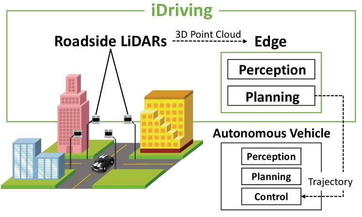
Figure 1. Autonomous vehicles run perception, planning and control on-board. iDriving augments autonomous driving; it runs perception and planning on edge-compute infrastructure, and transmits trajectories directly to an autonomous vehicle’s control module.

iDriving can help improve safety and traffic throughput at intersections. Annually, in the US, about 2.5 million accidents occur at intersections, which contribute to 50% of all serious accidents and 25% of fatalities [19]. As such, intersections are a focus area for the US Federal Highway Administration (FHWA) [21] with programs that improve current intersection designs and explore safer alternatives. Intersection safety is a challenge problem for autonomous vehicles as well [31] because of line-of-sight limitations [72]. In addition, wait times at intersections in major metropolitan areas can be significant, and higher traffic throughput can result in reduced wait times. A recent report [17] estimates that drivers in California spend, on aggregate, 2.7M hours in a 24-hour period waiting at intersections!

iDriving has two properties that enable it to address these problems at intersections:

1. LiDARs mounted at each corner of an intersection above car heights can get a comprehensive view of all vehicles and traffic participants at an intersection (Fig. 1). This improved perspective can help overcome safety issues caused by line-of-sight limitations. Consider Fig. 2, which illustrates a common and deadly safety issue at intersections: red-light violations, which account for 700-800 fatalities in the US annually [19]. In this figure, the yellow vehicle’s view of the red-light violator (the blue car) is blocked by a red truck. This scenario is known to be challenging for autonomous vehicles [31] as well. iDriving, because it notices the blue car, can generate a trajectory for the yellow vehicle to cause it to slow down, and thereby avoid a collision.

2. Because it jointly plans trajectories for all autonomous vehicles, at an intersection, iDriving can increase traffic throughput and even enable traffic-light free intersections [88]. To see why, consider the same scenario as in Fig. 2, but now suppose that all vehicles are autonomous. Also suppose there are no traffic lights at the intersection. Then, as the vehicles arrive, iDriving can develop trajectories that slow down the blue car or speed up the red truck and the yellow car (or both), so that all cars can safely traverse the intersection. More important, joint trajectory planning is necessary to achieve this capability. If iDriving had only offloaded perception to infrastructure (which provides comprehensive views of traffic analogous to cooperative perception in AVR [72] or EMP [102]), and left it to vehicles to plan trajectories based on its scene description, traffic can deadlock (§4.6), resulting in zero throughput.

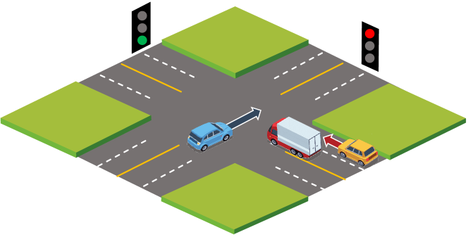
Figure 2. How iDriving works in a scenario from CarLA [41]. Roadside LiDARs transmit data over a wired network to an edge cluster. iDriving’s perception extracts vehicles and their motion information, and its planning component determines that the blue vehicle can safely pass the stalled vehicle. iDriving wirelessly delivers a trajectory designed for the blue vehicle, whose control component executes the trajectory.

iDriving Challenge. iDriving has stringent bandwidth, latency, accuracy and robustness requirements, and it must be possible to meet these requirements on commodity hardware deployed on edge computing infrastructure.

• LiDARs generate data at 10 frames per second. At 30 MB per frame, this translates to a raw data rate of nearly 10 Gbps for four LiDARs at an intersection. LiDARs can have wired network connections so the network is unlikely to be a bottleneck, but extracting scene understanding from voluminous data can stress compute.

• iDriving must produce trajectories within a tight latency (time taken to run a single frame from each LiDAR through its perception and planning) constraint. Industry players like Udacity [1], Mobileye [82, 83], and Tesla [23] argue that autonomous vehicles must make decisions with a tail latency of less than 100 ms. Other work exploring autonomous driving also suggests the same constraint [59].

• iDriving generates scene descriptions which consist of objects, their tracks, positions, heading, and speed. The accuracy of these quantities, must match or exceed the state-of-the-art.

• iDriving transmits trajectories wirelessly, and this must be robust to packet losses.

Strategy	Perception	Planning	Perf	Sfty	Tput
AVR [72]	Cooperative (V2V)	On-board	?	✘	✘
EMP [102]	Cooperative (V2I)	On-board	?	✘	✘
VI-Eye [51]	Cooperative (I-V)	On-board	✘	✘	✘
Autocast [73]	Cooperative (V2V)	On-board	✔	✔	✘
iDriving	Infrastructure	Infrastructure	✔	✔	✔

Table 1. Comparison to related work. Perf refers to achieving 100 ms end-to-end tail latency. A ? in this column suggests that the work has partially benchmarked performance (e.g., only perception) and this is within 100 ms. Sfty indicates whether the work has demonstrated safety in evaluations, and Tput indicates whether the work has demonstrated throughput in evaluations. In this paper, we show that, in certain cases, cooperative perception can result in deadlock, resulting in poor throughput.

It is not immediately obvious that iDriving can meet these requirements; for instance, the most accurate 2D and 3D object detectors on the KITTI leaderboard [47] incur a processing latency of 60-300 ms!

Contributions. To address these challenges, we make the following contributions:

• iDriving incorporates a novel stack for perception and planning, which is qualitatively different from existing autonomous driving stacks (§2).

• Its perception pipeline fuses multiple LiDAR outputs using a novel alignment algorithm whose accuracy is significantly higher than prior work (§2.2).

• Accurate alignment enables fast and cheap implementation of object extraction, tracking, and speed estimation, all centered around a single bounding box abstraction computed early in the pipeline (§2.3).

• However, cheap algorithms for estimating heading are inaccurate, so iDriving develops a more accurate heading estimator, and offloads this to a GPU to meet the latency constraint (§2.4).

• iDriving adapts an existing fast single-robot motion planner to jointly plan trajectories for multiple vehicles, and to account for real-world non-idealities, and wireless packet loss (§3).

		iDriving	Baidu Apollo [15]	Autoware [63]
Perception	Mapping	None	Pre-built HD-Map	Pre-built HD-Map
	Localization	Live Fused Point Cloud (§2.2)	LiDAR scan matching fused with GPS-RTK and IMU	LiDAR scan matching
	Object detection	3D Object Detection (§2.3)	Obstacle detection in 2D BEV projection	2D object detection in camera, projected to 3D
	Tracking and motion estimation	Kalman filter with matching, Heading Estimation (§2.4)	Kalman filter with matching	Kalman filter with matching
Planning		Centralized Interval Planner (§3)	Ego-planner using hybrid A$\star$ search	Ego-planner using conformal lattices

Table 2. iDriving uses a qualitatively different stack to meet throughput and latency requirements. Both perception and planning use different algorithms (highlighted in bold) than existing open-source stacks.

Summary of Results. Evaluations on a testbed, a deployment at a busy intersection in a large metropolitan city, and on a photorealistic autonomous driving simulator [41] validate these contributions and demonstrate its superiority relative to today’s autonomous driving and to cooperative perception (§4). iDriving achieves its performance objectives end-to-end, being able to process frames from 4 LiDARs at 10 fps with a 99-th percentile tail latency under 100 ms. Its perception component can track vehicles to centimeter-level accuracy (comparable to SLAM [100]-based positioning). Its planner ensures safe passage in all red-light violation and unprotected left-turn scenarios, while autonomous driving can do so only 27% of the time. It can reduce wait times 5$\times$ at intersections relative to intelligent traffic lights; in contrast, cooperative perception (e.g., [72, 73, 102]) can result in deadlock.

Related Work. iDriving falls into a qualitatively different point in the design space relative to the most closely related prior work (Tbl. 1); it is the first to explore completely moving perception and planning to the infrastructure. It is also the first to consider safety and throughput. Several pieces of work have considered various forms of cooperative perception. AVR [72] and Autocast [73] use vehicle-to-vehicle cooperative perception, EMP [102] uses edge compute infrastructure, and Vi-Eye [51] in addition uses infrastructure sensors. All of these approaches rely on on-board planning. Of these, only Autocast [73] demonstrates end-to-end performance (including perception and planning) and safety, but does not evaluate throughput. In this paper, we show that even with comprehensive views of traffic (as with cooperative perception), on-board planning can result in zero throughput in some cases due to deadlock.

2. Perception

iDriving consists of two components (Tbl. 2): perception and planning. In this section, we describe the former.

2.1. Perception Overview

Inputs and Outputs. The input to perception is a continuous sequence of LiDAR frames from each LiDAR in a set of overlapping LiDARs deployed roadside. To ground the discussion, consider four LiDARs deployed at an intersection. Fig. 3(a) shows a view of a busy intersection in a major metropolitan area. At this intersection, we mounted LiDARs at the four corners (§4).

The output of perception is a compact abstract scene description: a list of bounding boxes of moving objects in the environment together with their motion vectors (Fig. 3(e)). This forms the input to the planner (§3), which also requires other inputs that we describe later.

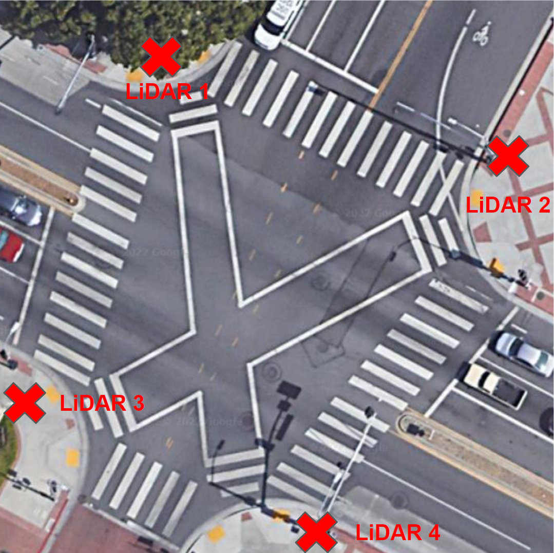
(a)

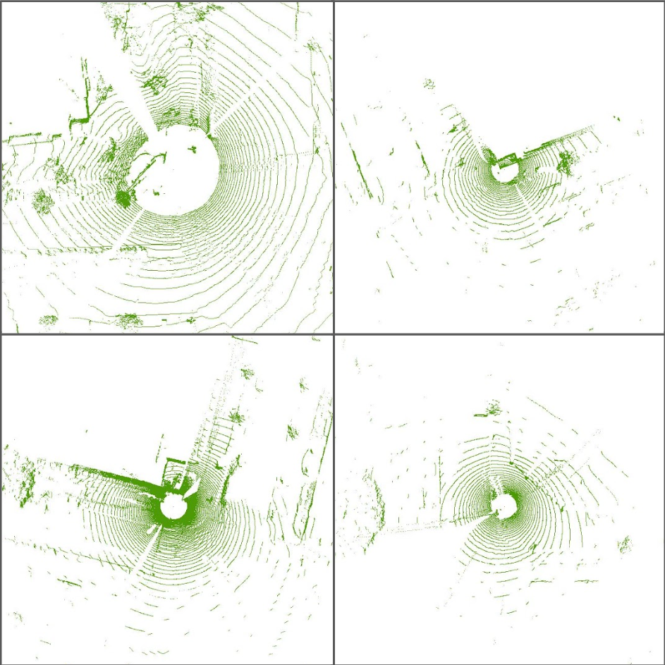
(b)

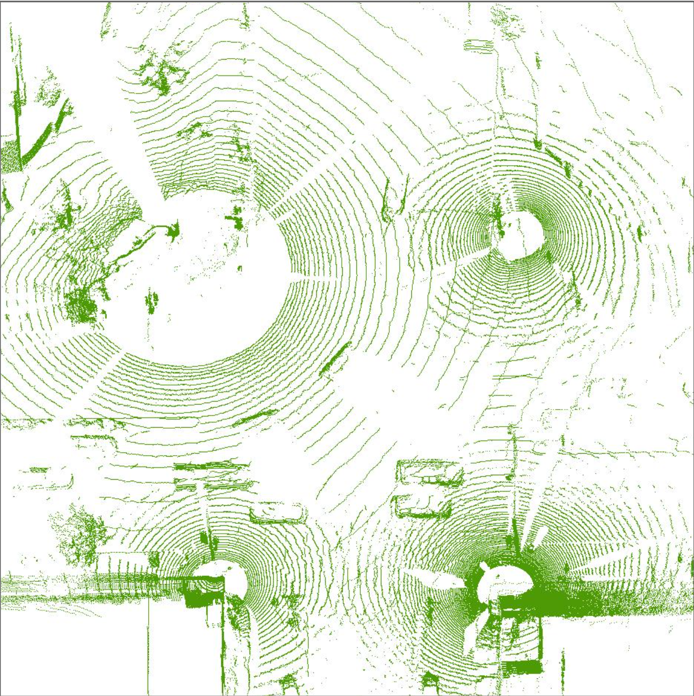
(c)

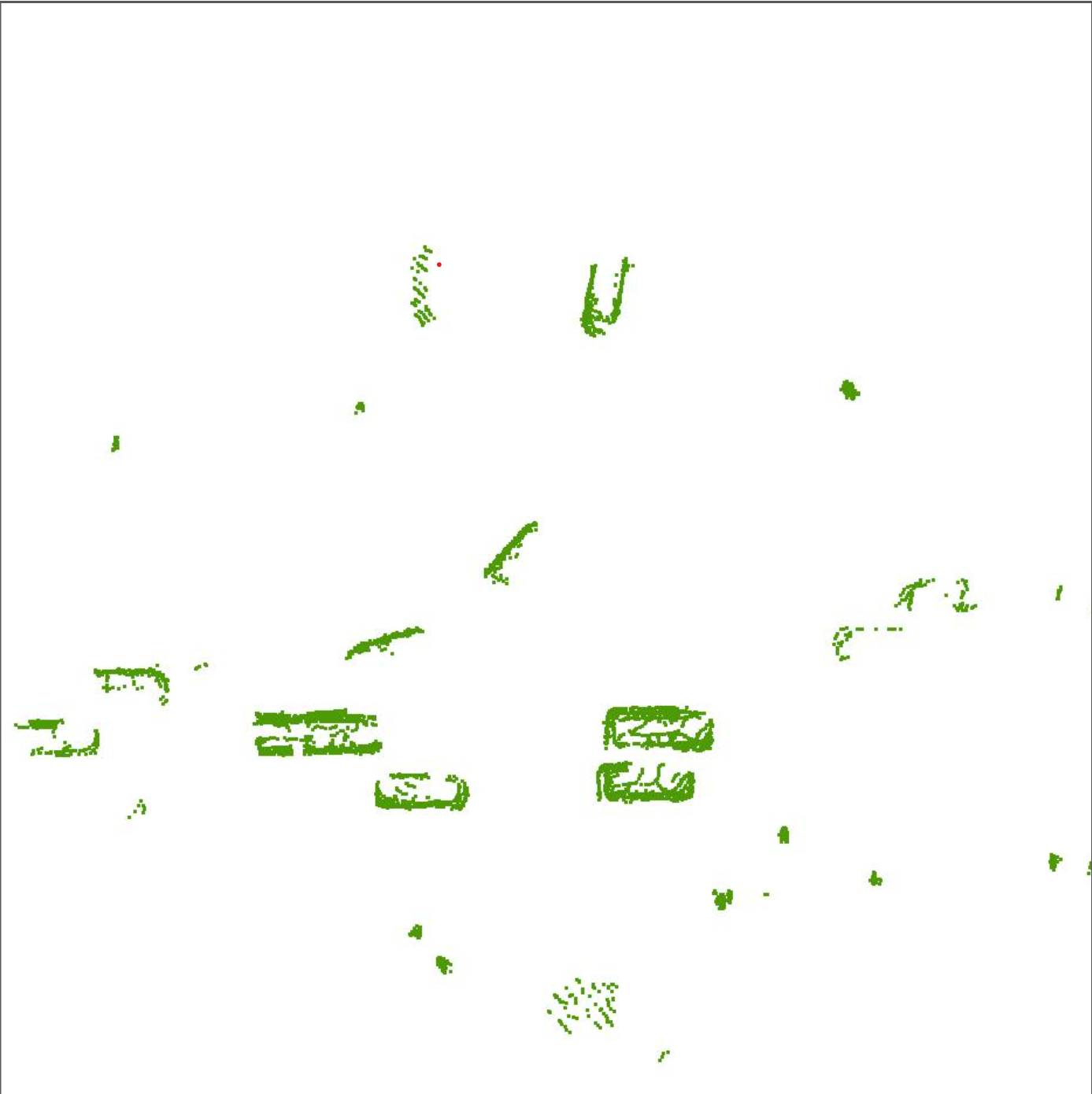
(d)

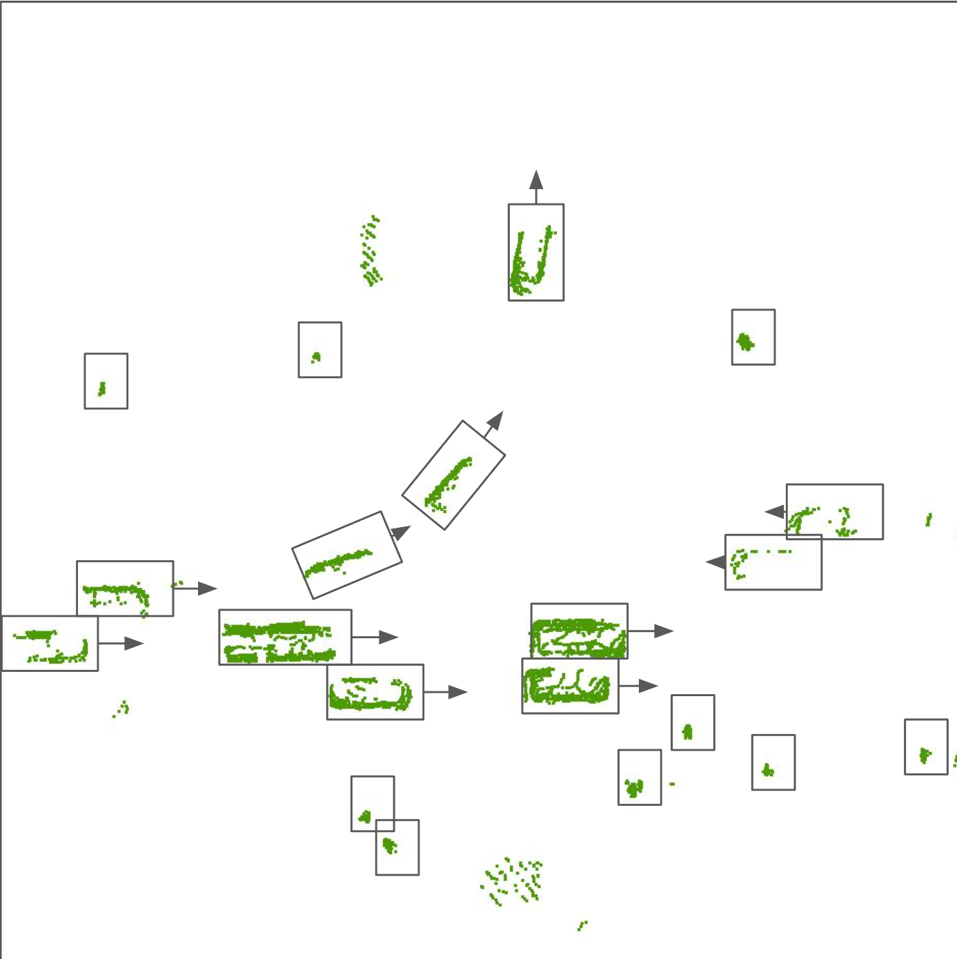
(e)

Figure 3. iDriving deployment at a busy intersection with heavy vehicular and pedestrian traffic in a large metropolitan city. (a) A top down view of the intersection (taken from Google Maps [2]. We mounted four LiDARs near each of traffic light poles situated at the four corners of the intersection. (b) An individual frame from each one of the 4 LiDARs. (c) A fused frame. (d) Point clouds of traffic participants (dynamic objects) at the intersection. (e) Bounding boxes and motion vectors for traffic participants, calculated over successive frames.

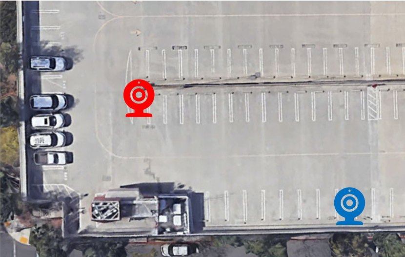
(a)

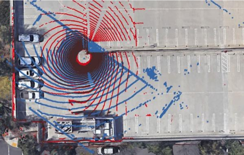
(b)

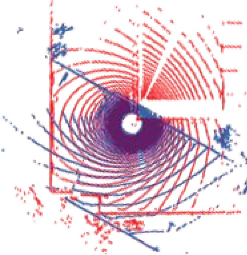
(c)

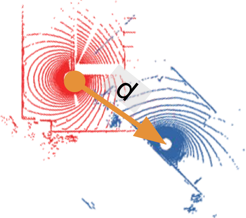
(d)

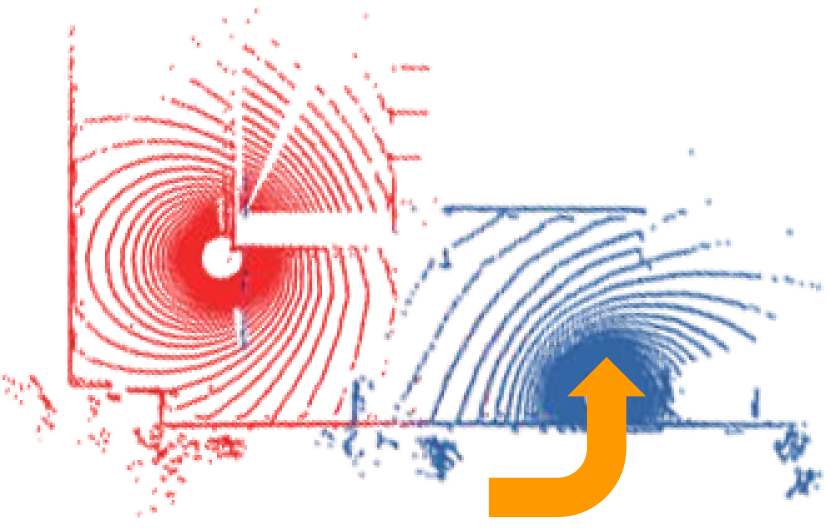
(e)

Figure 4. An illustration of iDriving’s point cloud alignment algorithm. (a) A top down view of a parking lot with two LiDARs shown by red ($L_{1}$) and blue ($L_{2}$) icons. (b) The inputs to initial guess algorithm are point clouds ($C_{1}$ and $C_{2}$) in the respective LiDAR’s coordinate system along with the ground distance $d$ between them. (c) Figure (b) with background removed. (d) To fix the base coordinates, iDriving displaces $C_{2}$ by the ground distance $d$. (e) iDriving rotates both $C_{1}$ and $C_{2}$ by small yaw increments to find the combination with the lease distance between the point clouds.

Approach. To address the challenges described in §1, iDriving’s perception uses a three stage pipeline, each with three sub-stages (Fig. 5). Fusion combines multiple LiDAR views into fused frames, and then subtracts the static background to reduce data. Participant extraction identifies traffic participants by clustering and estimates a tight 3D bounding box around each object. Tracking associates objects across frames, and estimates their heading and motion vectors.

This design achieves iDriving’s goals using three ideas:

• iDriving exploits the fact that LiDARs are static to cheaply fuse point clouds from multiple overlapping LiDARs into a single fused frame. Such a frame may have more complete representations of objects than individual LiDAR frames. Fig. 3(b) shows the view from each of the 4 LiDARs; in many of them, only parts of a vehicle are visible. Fig. 3(c) shows a fused frame which combines the 4 LiDAR frames into one; in this, all vehicles are completely visible.

• iDriving builds most algorithms around a single abstraction, the 3D bounding box of a participant (Fig. 3(e)). Its tracking, speed estimation, and motion vector estimation rely on the observation that the centroid of the bounding box is a convenient consistent point on the object for estimating these quantities, especially when fused LiDAR frames provide comprehensive views of an object.

• iDriving uses, when possible, cheap algorithms rather than expensive deep neural networks (DNNs). Only when higher accuracy is required does iDriving resort to expensive algorithms, but employs hardware acceleration to meet the latency budget; its use of a specialized heading vector estimation algorithm is an example.

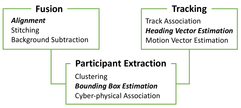
Figure 5. Perception stages and sub-stages. We describe sub-stages in bold in detail.

Qualitative Design Comparison. iDriving’s perception design is qualitatively different (Tbl. 2) from that of other popular open-source autonomous driving stacks, Baidu’s Apollo [15] and Autoware [63]:

• These approaches [15, 63] rely on a pre-built HD-map, and localize the ego-vehicle (the one on which the autonomous driving stack runs) by matching its LiDAR scans against the HD map (Apollo additionally improves position estimates using multi-sensor fusion). In contrast, iDriving does not require a map for positioning: all vehicle positions can be directly estimated from the fused frame.

• Autonomous driving stacks use different ways to identify traffic participants. Apollo extracts obstacles on a 2D occupancy grid and infers participants from contiguous occupied grids. Autoware uses camera images and uses 2D object detector DNNs, then back-projects these to the 3D LiDAR view. In contrast, iDriving directly extracts the 3D point cloud associated with each participant. It can do this cheaply using background subtraction because its LiDARs are static.

• Autonomous driving stacks use Kalman filters to estimate motion properties (speed, heading) of other vehicles. For heading, iDriving uses a more sophisticated algorithm to ensure higher tail accuracy.

We now describe parts of iDriving’s novel perception relative to autonomous driving stacks (bold text in Tbl. 2).

2.2. Accurate Alignment for Fast Fusion

Point Cloud Alignment. Each frame of a LiDAR contains a point cloud, a collection of points with 3D coordinates. These coordinates are in the LiDAR’s own frame of reference. Fusing frames from two different LiDARs is the process of converting all 3D coordinates of both point clouds into a common frame of reference. Alignment computes the transformation matrix for this conversion.

Prior work has developed Iterative Closest Point (ICP) [36, 27] techniques that search for the lowest error alignment. The effectiveness of these approaches depends upon the initial guess for LiDARs’ poses. Poor initial guesses can result in local minima. SAC-IA [79] is a well-known algorithm to quickly obtain an initial guess for ICP. As we demonstrate in §4, with SAC-IA’s initial guesses, ICP generates poor alignments on full LiDAR frames.

Initial guesses using minimal information. Besides the 3D point clouds, SAC-IA requires no additional input. We have developed an algorithm to obtain good initial guesses (that enable highly accurate ICP alignments) using minimal additional input. Specifically, iDriving only needs the distances on the ground (using, for example, an off-the-shelf laser rangefinder) between a reference LiDAR and all others to get good initial guesses. We now describe the algorithm for two LiDARs $L_{1}$ and $L_{2}$ (as shown in Fig. 4(a)); the technique generalizes to multiple LiDARs, as described in Algorithm 1.

The inputs are two point clouds $C_{1}$ and $C_{2}$ (more generally, $N$ point clouds, Algorithm 1) captured from the corresponding LiDARs at the same instant (Fig. 4(b) and Fig. 4(c)), and the distance $d$ on the ground between the LiDARs. The output is an initial guess for the pose of each LiDAR. We feed these guesses into ICP to obtain good alignments. The algorithm conceptually consists of three steps:

Fixing the base coordinates.

Without loss of generality, set LiDAR $L_{1}$’s $x$ and $y$ coordinates to be $(0,0)$ (i.e., the base is at the origin). Then, assume that $L_{2}$’s base is at $(d,0)$ (Fig. 4(d)).

Estimating height, roll and pitch.

In this step, we determine: the height of each LiDAR $z_{i}$, the roll (angle around the $x$ axis), and pitch (angle around the $y$ axis). For these, iDriving relies on fast plane-finding algorithms [40] that extract planes from a collection of points (lines 1 and 1 of Algorithm 1). These techniques output the equations of the planes. Assuming that the largest plane is the ground-plane (a reasonable assumption for roadside LiDARs), iDriving aligns the $z$ axis of two LiDARs with the normal to the ground plane (line 1). In this way, it implicitly fixes the roll and pitch of the LiDAR. Moreover, after alignment, the height of the LiDARs $z_{i}$ is also known (because the $z$ axis is perpendicular to the ground plane).

Estimating yaw.

Finally, to determine yaw (angle around the $z$ axis), we use a technique illustrated in Fig. 4(e) (line 1 of Algorithm 1). In this technique, iDriving rotates both point clouds $C_{1}$ and $C_{2}$ with different yaw settings until it finds a combination that results in the smallest 3D distance between the two point clouds. We have found that ICP is robust to initial guesses for yaw that are within about 15-20^∘ of the actual yaw, so iDriving discretizes the search space by this amount. In case of Fig. 4(e), iDriving calculates the initial guess for the yaw by rotating the blue point cloud ($C_{2}$).

iDriving repeats this procedure (lines 3-6) for every other LiDAR $L_{i}$ with respect to $L_{1}$, to obtain initial guesses for the poses of every LiDAR. It feeds these into ICP to obtain an alignment.

Re-calibrating alignment. Because alignment is expensive, it is run only once, when installing the LiDARs. Re-alignment may be necessary if a LiDAR is replaced or re-positioned. Alignment is performed infrequently but is crucial to iDriving’s accuracy (§4.4).

Using alignment: Stitching. LiDARs generate frames at 10 fps (or more). In Fig. 3, when each LiDAR generates a frame, the fusion stage performs stitching. Stitching applies the coordinate transformation for each LiDAR generated by alignment, resulting in a fused frame (Fig. 3(c)).

1

Input : 1. $\mathbf{C}=\{C_{1},\cdots,C_{N}\}$; $C_{i}$ is LiDAR $L_{i}$’s point cloud.
2. $D=\{d_{2},\cdots,d_{N}\}$; $d_{i}$ is the distance from $L_{i}$ to the reference LiDAR $L_{1}$.

Output : $T=\{T_{2},T_{3},\cdots,T_{N}\}$; $T_{i}$ is the transformation to translate $C_{i}$ to $L_{1}$’s coordinate system.

2

3SegmentGroundPlane ( $C_{1}$ );

4

5for $i\leftarrow 2$ to $N$ by $1$ do

6      

7      SegmentGroundPlane ( $C_{i}$ );

8      

9      AlignGroundPlane ( $C_{i}$, $C_{1}$ );

10      

11      AlignPosition ( $C_{i}$, $C_{1}$, $d_{i}$ );

12      

13      EstimateYaw ( $C_{i}$ );

14      

15 end for

Algorithm 1 Estimating an initial guess for alignment

2.3. Reusing 3D Bounding Boxes

iDriving’s efficiency results from re-using the 3D bounding box of a participant (Fig. 3(e)) in many processing steps. After stitching, iDriving extracts the bounding box by performing background subtraction on the fused point cloud to extract points belonging to moving objects, then applies clustering techniques to determine points belonging to individual objects, and run a bounding box estimation algorithm. These use well-known algorithms, albeit with some optimizations; we describe these in §2.5.

Using the 3D Bounding Box. iDriving uses the bounding box for many of its algorithms (Tbl. 3). Accurate alignment enables low complexity algorithms that use the pre-computed bounding box geometry. These algorithms are key to achieving low latency perception without compromising accuracy.

• To associate objects across frames (tracking), it uses a Kalman filter to predict the position of the centroid of the 3D bounding box, then finds the best match (in a least-squares sense) between predicted positions and the actual positions of the centroids in the frame. Although tracking in point clouds is a challenging problem [92] for which research is exploring deep learning, a Kalman filter works exceedingly well in our setting. The biggest challenge in tracking is occlusions: when one object occludes another in a frame, it may be mistaken for the other in subsequent frames (an ID-switch). Because our fused frame includes perspectives from multiple LiDARs, ID-switches occur rarely (in our evaluations, §4).

• To estimate speed of a vehicle, iDriving measures the distance between the centroid of the bounding box in one frame, and the centroid $w$ frames in the past ($w$ is a configurable window size parameter), then estimates speed by dividing the distance by the time taken to generate $w$ frames.

• iDriving needs to associate an object seen in the LIDAR with a cyber endpoint (e.g., an IP address) so its planning component can send a customized trajectory to each vehicle. For this cyber-physical association (Fig. 5), iDriving uses a calibration step performed once. In this step, given a vehicle for which we know the cyber-physical association (e.g., a LiDAR installer’s vehicle), we estimate the transformation between the trajectory of the vehicle seen in the LiDAR view with the GPS trajectory (we omit the details for brevity). When iDriving runs, it uses this to transform a vehicle’s GPS trajectory to its expected trajectory in the scene, then matches actual scene trajectory to expected trajectory in a least-squares sense. To define the scene trajectory, we use the centroid of the bounding box of the vehicle.

Centroid			Axes	Dimension
Tracking	Speed Estimation	Cyber-Phy Association	Heading Estimation	Planning

Table 3. iDriving computes bounding boxes for traffic participants early on and reuses properties of the bounding boxes in multiple modules to ensure low latency.

In all of these tasks, the centroid of the bounding box is an easily computed, consistent, point within the vehicle that aids these tasks. Moreover, because we have multiple LiDARs that capture a vehicle from multiple directions, the centroid of the bounding box is generally a good estimate of the actual centroid of the vehicle.

Besides these, iDriving (a) estimates heading direction from the axes of the bounding box (discussed in §2.4) and (b) uses the dimensions of the box to represent spatial constraints for planning (discussed in §3).

2.4. Fast, Accurate Heading Vectors

Planning also needs the motion vector to predict trajectories for vehicles. To compute this, iDriving first determines, for each object, its instantaneous heading (direction of motion), which is one of the three surface normals of the bounding box of the vehicle. It estimates the motion vector as the average of the heading vectors in a sliding window of $w$ frames. Most autonomous driving stacks can obtain heading from SLAM or visual odometry (§5), so little prior work has explored extracting heading from infrastructure LiDAR frames.

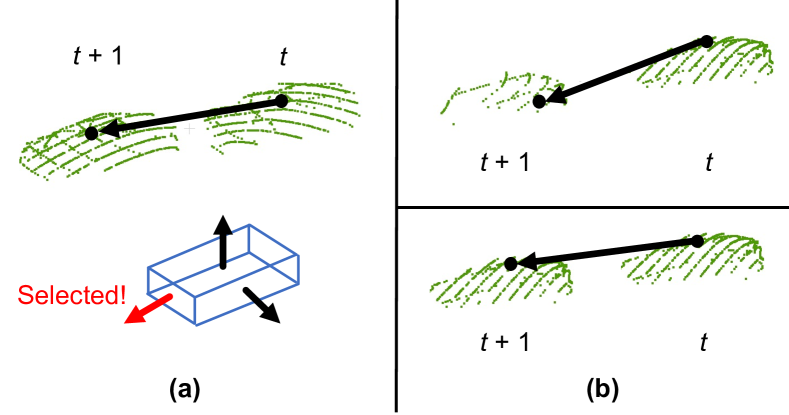
Figure 6. The figure shows the points belonging to a car, in two successive frames $t$ and $t+1$. (a) Strawman approach for heading determination. (b) iDriving’s approach.

A strawman approach. Consider an object $A$ at time $t$ and time $t+1$. Fig. 6(a) shows the points belonging to that object. Since those points are already in the same frame of reference, a strawman algorithm is: (a) find the vector between the centroid of $A$ at time $t$ and centroid of $A$ at time $t+1$, (b) the heading direction is the surface normal (from the bounding box) that is most closely aligned with this vector (Fig. 6(a)). We have found that the error distribution of this approach can have a long tail (although average error is reasonable). If $A$ has fewer points in $t+1$ than in $t$ (Fig. 6(b), upper), the computed centroid will be different from the true centroid, which can induce significant error.

iDriving’s approach. To overcome this, we (a) use ICP to find the transformation matrix between $A$’s point cloud in $t$ and in $t+1$, (b) “place” $A$’s point cloud from $t$ in frame $t+1$ (Fig. 6(b), lower), (c) then compute the vector between the centroids of these two (so that the centroid calculations are based on the same set of points). As before, the heading direction is the surface normal (from the bounding box) that is most closely aligned with this vector.

GPU acceleration. ICP is compute-intensive, even for small object point clouds. If there are multiple objects in the frame, iDriving must run ICP for each of them. We have experimentally found this to be the bottleneck, so we developed a fast GPU-based implementation of heading vector estimation, which reduces the overhead of this stage (§4.3).

A typical ICP implementation has four steps: (1) estimate correspondence between the two point clouds, (2) estimate transformation between two point clouds, (3) apply the transformation to the source point cloud and (4) check for the ICP convergence. The first step requires a nearest neighbor search; instead of using octrees, we adapt a parallelizable version described in [46] but use CUDA’s parallel scanning to find the nearest neighbor. The second step shuffles points in the source point cloud then applies the Umeyama [91] algorithm for the transformation matrix. We re-implemented this algorithm using CUDA’s demean kernel, and a fast SVD implementation [45]. For the third and fourth steps, we developed custom CUDA kernels.

2.5. Other Details

Background Subtraction. This step removes points belonging to static parts of the scene, is (a) especially crucial for voluminous LiDAR data and (b) feasible in our setting because the LiDARs are static. It requires a calibration step to extract a background point cloud from each LiDAR [55], then creates a background fused frame using the results from alignment; taking the intersection of a few successive point clouds and the aggregating intersections taken at a few different time intervals, works well to generate the background point cloud.

Optimization: background subtraction before stitching. iDriving subtracts the background fused frame from each fused frame generated by stitching. We have found that a simple optimization can significantly reduce processing latency: first removing the background from each LiDAR frame (using its background point cloud), and then stitching points in the residual point clouds. Stitching scales with the number of points, which this optimization reduces significantly.

Optimization: exploiting LiDAR characteristics. Many LiDAR devices only output returns from reflected laser beams. Generic background subtraction algorithm requires a nearest-neighbor search to match a return with the corresponding return on the background point cloud. Some LiDARs (like the Ouster), however, indicate non-returns as well, so that the point cloud contains the output of every beam of the LiDAR. For these, it is possible to achieve fast background subtraction by comparing corresponding beam outputs in a point cloud and the background point cloud.

At the end of these two steps, the fused frame only contains points belonging to objects that are not part of the scene’s background (Fig. 3(d)).

Computing the 3D bounding box. On the points in the fused frame remaining after background subtraction, iDriving uses a standard, fast, clustering algorithm (DBSCAN) [43] to extract multiple clusters of points, where each cluster represents one traffic participant. Then, it uses an off-the-shelf algorithm [4], which determines a minimum oriented bounding box (Fig. 3(d)) of a point cloud using principal component analysis (PCA). From these, we can extract the three surface normals of the object (e.g., vehicle): the vertical axis, the axis in the direction of motion, and the lateral axis.

3. Planning

Inputs, Outputs, and Goals. From perception, iDriving’s planner receives bounding boxes for non-background objects, and their motion vectors. Some of these objects will be iDriving-capable vehicles; these follow trajectories designed by iDriving. For these, iDriving needs each vehicle’s navigation goal, e.g., where it is headed: we assume the planning component can get this by communicating with the vehicle. Other objects will be iDriving-oblivious: these include pedestrians, or vehicles driven by humans or on-board autonomous driving agents. The output of planning is a trajectory — a sequence of way-points, and times at which those way-points should be reached — for each iDriving-capable vehicle.

Planning executes at every frame and must satisfy two goals: (a) it must fit within the tail latency budget of 100 ms, (b) and it must generate collision-free trajectories at every instant even in the presence of iDriving-oblivious objects.

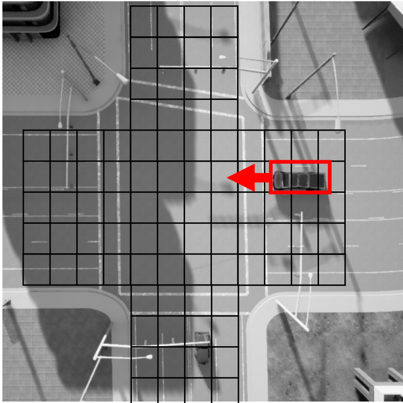
(a)

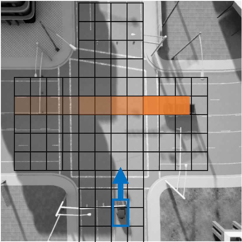
(b)

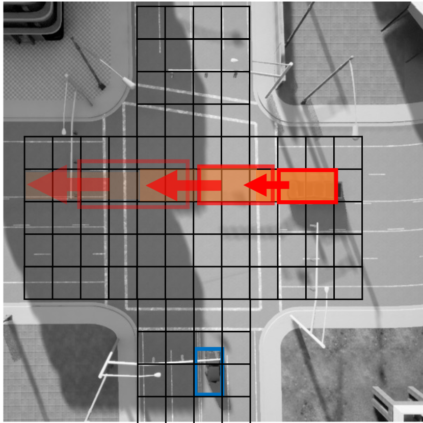
(c)

Figure 7. (a) The first (red) planned vehicle can use the entire drivable space. (b) The second (blue) vehicle treats the first as an obstacle (different shades represent different times at which grids are occupied). (c) The motion-adaptive buffer around a vehicle is proportional to its speed.

iDriving’s Planner. The best-known centralized robot motion planner, Conflict Based Search [84] that jointly optimizes paths for multiple robots, has high tail latency [24, 70]. Instead, we use a fast single-robot motion planner, SIPP [70]. The input to SIPP is a goal for a robot and the positions over time of the dynamic obstacles in the environment. The output is a provably collision-free shortest path for the robot [70].

At each frame, iDriving must plan trajectories for every iDriving-capable vehicle. Without loss of generality, assume that vehicles are sorted in some order. iDriving’s centralized planner iteratively plans trajectories for vehicles in that order:

When running SIPP on the $i$-th vehicle, iDriving represents all $i-1$ previously planned vehicles as dynamic obstacles in SIPP.

Fig. 7(b) illustrates this, in which the trajectory of a previously planned (red) vehicle is represented as an obstacle when planning a trajectory for the blue vehicle.

This approach has two important properties:

1. All trajectories are collision-free. Two cars $i$ and $j$ cannot collide, since, if $j>i$, $j$’s trajectory would have used $i$’s as an obstacle, and SIPP generates a collision-free trajectory for each vehicle.

2. iDriving’s planner cannot result in a traffic deadlock. A deadlock occurs when there exists a cycle of cars in which each car’s forward progress on its currently planned trajectory is hampered by another. Fig. 8 shows examples of deadlocked traffic with two, three, and four cars (these scenarios under which these deadlocks occurred are described in §4.6). However, iDriving cannot deadlock. If there exists a cycle, there must be at least one pair of cars $i,j$ where $i<j$ and $i$ blocks $j$. But this is not possible, because, when planning for $j$, iDriving represents $i$’s trajectory as an obstacle.

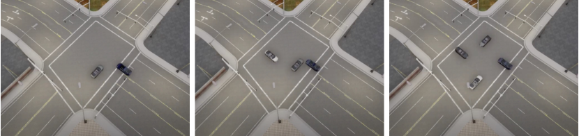
Figure 8. With autonomous driving’s decentralized planning, in the absence of a traffic light controller, vehicles come to a deadlock at the intersection where they are unable to cross it.

However, this approach may sacrifice optimality in transit times: vehicles later in the planning order may see longer transit times. On the flip side, it may allow iDriving to achieve novel traffic policies (e.g., those that prioritize emergency vehicles). Future work can explore such traffic policies.

Because it was designed for robots, SIPP makes some idealized assumptions. iDriving adapts SIPP to relax these.

Robustness to iDriving-oblivious participants. SIPP plans the entire trajectory for a robot once, given all the dynamic obstacles in the environment. iDriving, to deal with iDriving-oblivious vehicles whose trajectories can change dynamically, re-plans trajectories for every iDriving-capable vehicle at every frame. This also relaxes assumption in SIPP that all objects move at a fixed speed. For each iDriving-oblivious object, iDriving uses its bounding box, and motion and heading vector.

Robustness to perception errors. SIPP assumes that each object has the same size, occupying one grid element. To relax this to permit different vehicle sizes (cars, trucks), iDriving uses the bounding boxes generated by perception to determine grid occupancy. Because these bounding boxes may be incorrect, iDriving extends the bounding box by a small buffer on all sides. This extended buffer is motion-adaptive: the faster the vehicle travels the larger is the buffer around it (Fig. 7(c)).

Robustness to packet losses. The trajectory generated by iDriving is transmitted over a wireless network to the vehicle. To be robust to packet losses, iDriving generates waypoints over a longer horizon (10 s [83]) than the inter-frame time (100 ms in our case). This way, it transmits trajectories every 100 ms, but if a transmission is lost, the vehicle can use the previously-received trajectory.

Robustness to vehicle kinematics limitations. SIPP assumes that a vehicle can start and stop instantaneously. In practice, a vehicle’s kinematic characteristics dictate how quickly vehicles can start and stop. The longer planning horizon helps with the vehicle’s controller time to adapt to vehicle kinematics. The controller (on-board the vehicle) can determine, from the received trajectory, if it has to stop at some future point in time; it can then decide when to apply the brakes, and with what intensity, to effect the stop.

iDriving Extensions to On-board Control. Every iDriving-compatible vehicle has an on-board local low-level controller and PID controller that receives the set of planned way-points from the centralized planner over the network. The local controller translates these to low-level control signals (throttle, steer, and brake) that can be directly applied to each vehicle. The local controller runs every 2-3 ms in the vehicle.

The local controller receives the planned trajectory (for that vehicle) from the centralized planner every 100 ms. If it does not receive a trajectory from the centralized planner within a latency budget (e.g., due to network failure), it initiates a recovery mode, which uses the last valid trajectory received by the vehicle in a previous cycle. The local controller can afford to do this because the planner plans, and sends a trajectory for a longer time horizon (§3). It would have sufficed to send the vehicle its trajecotry for just the next 100 ms but instead, iDriving sends a trajectory for the next $x$ seconds. This redundancy in the design not only addresses network failures but also helps relax SIPP’s instant start/stop assumption and introduces robustness.

Given the planned trajectory for the next $x$ seconds, the local controller determines whether the vehicle has to wait at any point along its planned trajectory. We call this a wait cycle. If there is a wait cycle, it finds the position associated with the wait cycle and the distance of the vehicle from it. The controller then calculates the braking distance (distance to bring the vehicle to a complete stop) of the vehicle using its motion vector. If the braking distance is less than or equal to the distance from the stopping point, the controller generates a signal to apply brake. Without this, vehicles would apply brakes at the spatial position of the wait cycle and hence overshoot it. With this maneuver, iDriving ensures that vehicles can adhere to SIPP’s collision-free planned paths. On the other hand, if the vehicle is far away from the stopping point, then the controller generates a signal to continue moving the vehicle towards the stopping point. We calculate braking distance using a standard equation [3].

If there is no wait cycle in the entire trajectory, the controller selects the next suitable way-point and generates a signal to move the vehicle towards that way-point. Finally, the local controller applies the control signal to the vehicle.

4. Evaluation

Our evaluations show that iDriving: achieves frame rate processing and less than 100 ms tail latency both in real-world experiments (§4.2) and in simulation (§4.3); achieves accuracy comparable to prior work (§4.4); can be safer than autonomous driving (§4.5); and permits high-throughput traffic management (§4.6).

4.1. Methodology

Implementation. We implemented iDriving’s perception and planning on the Robot Operating System (ROS [74]). ROS provides inter-node (ROS modules are called nodes) communication using publish-subscribe, and natively supports points clouds and other data types used in perception-based systems. iDriving’s perception component runs as a ROS node that subscribes to point clouds, processes them as described in §2, and publishes the results. iDriving’s planner builds on top of an open-source SIPP implementation [95], runs as a ROS node, subscribes to the perception results, and publishes trajectories for each vehicle. Perception requires 6909 lines of C++ code, and planning 3800.

Real-world Testbed. Our testbed consists of four Ouster LiDARs [67] (an OS-1 64, an OS-0 128, and two OS-0 64). Three of these have a field of view of $90^{\circ}$ while the last one has a $45^{\circ}$ field of view. iDriving is designed to accommodate this sensor heterogeneity. The testbed also includes an edge computing unit with an AMD 5950x CPU (16 cores, 3.4 GHz) and a GeForce RTX 3080 GPU; iDriving’s planning and perception components run on this. The LiDARs and the edge computing unit connect through Ethernet cables and an Ethernet switch (using an off-the-shelf Wi-Fi access point). Finally, iDriving transmits trajectories to an in-vehicle Raspberry Pi 3 over Wi-Fi (as a proxy for 5G).

Simulation. In our testbed, iDriving-derived trajectories cannot be used to control vehicles, since vehicular control systems are proprietary. So, we complement our evaluations with a simulator which incorporates vehicular control. The simulator also helps us explore scaling of perception and planning. We use CarLA [41], an industry-standard photo-realistic simulator for autonomous driving perception and planning. It contains descriptions of virtual urban and suburban streets, and, using a game engine, can (a) simulate the control of vehicles in these virtual worlds, and (b) produce LiDAR point clouds of time-varying scenes within these virtual worlds. Unless otherwise noted, our simulation based evaluations focus on intersections; several challenge scenarios for autonomous driving focus on intersections [66, 31].

Metrics. We quantify end-to-end performance in terms of the 99th percentile of the latency (p99 latency) between when a LiDAR generates a frame, and when the vehicle receives the trajectory corresponding to that frame. To quantify accuracy of individual perception components, we use metrics described in prior work (defined later). We quantify planning efficacy by the rate of safety violations, or of undesirable outcomes such as deadlock.

Comparison. Relative to autonomous driving, iDriving’s perception has a more comprehensive scene understanding and can jointly plan for multiple vehicles at a time. To quantify this, we compare it against autonomous driving.

4.2. Real-world Experiment

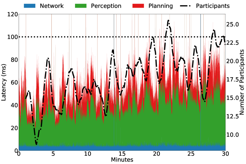
Figure 9. Per-component end-to-end latency (left y-axis) along with the number of traffic participants (right y-axis) from a deployment of iDriving at a busy intersection in the real-world for over 30 minutes. A p99 latency of 91 ms suggests that iDriving stays within the 100 ms latency budget (dotted line) for autonomous driving.

Deployment. We deployed our testbed at a busy four-way intersection with heavy pedestrian and vehicular traffic in a large metropolitan area. For this experiment, we deployed the four LiDARs at the corners of the intersection (Fig. 3(a)). These LiDARs connected to the edge compute device (described above) using Ethernet cables. The edge compute connected to Raspberry Pis on the vehicles through Wi-Fi (to proxy 5G). We collected data for nearly 30 minutes; we measured and report the end-to-end latency for every frame.

Results. Fig. 9 shows the end-to-end latency for each frame, for over 30 minutes (approximately 18,000 frames), broken down by component. The average end-to-end latency is 57 ms and p99 latency is 91 ms. This shows that iDriving operates under the 100 ms latency budget set for autonomous driving by industry players like Udacity [1], Mobileye[82], and Tesla [23]. Moreover, iDriving processed LiDAR input at full frame rate. This is encouraging, and suggests that it is possible to achieve end-to-end performance with iDriving comparable to those in today’s autonomous driving. Lastly, unlike autonomous driving pipelines today which control only a single vehicle, iDriving can control 10s of vehicles simultaneously within the 100 ms latency budget.

On average, at any given frame, iDriving detects 18 traffic participants (vehicles, pedestrians and cyclists) at the intersection during our experiment. As our experiment progressed, the traffic at the intersection steadily increased as shown by the dotted line in Fig. 9 (representing the running average of traffic participants for 600 frames or 60 seconds). Because iDriving’s latency depends on the number of traffic participants, this contributed to the slow increase in end-to-end latency towards the end of the experiment.

From this graph, we also observe that: network latency is small i.e., the average is 9 ms whereas p99 is 17 ms. The same is true for planning latency for which the average is 11 ms and p99 is 26 ms. Planning latency scales with the number of vehicles. As the number of vehicles increase through the course of the experiment, planning latency also increases. However, overall, perception latency (37 ms average and p99 of 60 ms) dominates, which motivates the careful algorithmic and implementation choices in §2.

4.3. Latency Breakdown

Setup. To explore the total latency with more vehicles, and to understand the breakdown of latency by component, we designed several scenarios in CarLA with increasing numbers of vehicles traversing a four-way intersection. In these scenarios, CarLA (a) generates LiDAR data and (b) controls vehicles based on received trajectories; the results use the same iDriving code used in the real-world experiment. To control vehicles, we set the steer, brake and throttle values of a vehicle, exposed through the CarLA API.

At this intersection, both streets have two lanes in each direction. We varied the number of vehicles from 2 to 14, to understand how iDriving’s components scale. To justify this range of the number of vehicles, we use the following data: the average car length is 15 ft [33], and the width of a lane is 12 ft [16]. Allowing for lane markers, medians, and sidewalks, let us conservatively assume that the intersection is 60 ft across. Suppose the intersection has traffic lights. Then, if traffic is completely stalled or moving very slowly, at most 4 cars can be inside the intersection per lane, resulting in a maximum of 16 cars (i.e., the maximum capacity of the intersection is 16). If cars are stalled, iDriving does not incur much latency since it doesn’t have to estimate motion, heading, or plan for these, so we limit our simulations to 14 vehicles. On the other hand, if traffic is moving at 45 mph (or 66 fps) and cars maintain a 3-second [38] safe following distance, then at most one car can be within the intersection per lane, for a total of 4 cars.

	Number of Vehicles
Component	2	4	7	10	12	14
Background Subtraction	7.5	8.9	9.9	9.9	11.0	18.7
Stitching	0.08	0.11	0.13	0.13	0.17	0.19
Clustering	4.3	5.8	11.2	13.0	22.2	20.5
Bounding Box	0.06	0.07	0.09	0.15	0.17	0.16
Tracking	0.1	0.15	0.21	0.28	0.37	0.38
Heading Vector	8.8	12.9	24.0	28.8	41.9	52.6
Total	18.5	26.4	43.7	47.1	69.9	81.5

Table 4. p99 per-frame latency (in milliseconds) for perception. We exclude latency numbers for motion vector estimation which are on the order of a few microseconds.

Breakdown for Perception. Tbl. 4 depicts the breakdown of 99-th percentile (p99) latency by component for perception, as well as the total p99 latency, as a function of the number of vehicles in the scene. In all our experiments, iDriving processed frames at the full frame rate (10 fps).

The total p99 latency for perception increases steadily up to 82 ms for 14 vehicles from 19 ms for 2 vehicles. This highlights the dependency of perception on scene complexity (§2); many components scale with the number of participants. At 14 vehicles, iDriving exceeds the latency budget, since planning requires over 20 ms for 14 vehicles (see below). These numbers suggest that modest off-the-shelf compute hardware that we have used in our experiments might be sufficient, at least for traffic management at moderately busy intersections. This data dependency also suggests that deployments of iDriving will need to carefully provision their infrastructures based on historical traffic (similar to network planning and provisioning).

The three most expensive components are background subtraction, clustering, and heading vector estimation. Background subtraction accounts for about 10 ms, but depends slightly on the number of vehicles; to be robust, it uses a filter (details omitted in §2.2) that is sensitive to the number of points (or vehicles). Clustering accounts for about 20 ms with 14 vehicles and is strongly dependent on the number of vehicles, since each vehicle corresponds to a cluster.

Heading vector estimation accounts for nearly 65% of perception latency, even after GPU acceleration (§2.4). These results show the fact that heading vector estimation is not only dependent on the number of vehicles, but their dynamics as well. When we ran perception on 16 vehicles, p99 latency actually dropped; in this setting, 16 vehicles congested the intersection, so each vehicle moved very slowly. Heading vector estimation uses ICP between successive object point clouds; if a vehicle hasn’t moved much, ICP converges faster, accounting for the drop.

Optimization	Before	After	Ratio
Background subtraction before stitching	67.7	10.0	6.7
Exploiting LiDAR characteristics	9.9	1.5	6.6
Heading vector GPU acceleration	1057.7	28.8	36.6

Table 5. Impact of optimizations on p99 latency

Other components are negligible. Stitching is fast because of the optimization described in §2.2. Bounding box estimation is inherently fast. Track association is cheap because it tracks a single point per vehicle (the centroid of the bounding box). Motion estimation is very fast (on the order of microseconds) and relies on positions computed during stitching. Thus, careful design choices that leverage abstractions and quantities computed earlier in the pipeline can be crucial for meeting latency targets (§2.4).

Benefits of optimizations. Tbl. 5 quantifies the benefits of our optimizations. Stitching before background subtraction requires nearly 70 ms in total; reversing the order reduces this time by 6.7$\times$. By exploiting LiDAR characteristics (§2.2), iDriving can perform background subtraction in 1.5 ms per frame. A CPU-based heading vector estimation requires nearly 1 s which would have rendered iDriving infeasible; GPU acceleration (§2.4) reduces latency by 35$\times$.

Calibration Steps. Finally, alignment (§2.2) of 4 LiDARs takes about 4 minutes. This includes not just the time to guess initial positions, but to run the ICP (on a CPU). Because it is invoked infrequently, we have not optimized it.

Planning. Tbl. 6 depicts the p99 planning latency. As expected, there is a dependency on the number of vehicles, since iDriving individually plans for each vehicle. Planning latencies can be slightly non-monotonic (the planning cost for 12 vehicles is more than that for 14) because the planner’s graph search can depend upon the actual trajectories of the vehicles, not just their numbers.

Number of Vehicles	2	4	7	10	12	14
p99 Latency (ms)	2.4	5.1	11.9	17.1	28.7	24.2

Table 6. p99 per-frame planning latency in milliseconds.

4.4. Accuracy

Perception Component Accuracy. Using real-world data and simulation traces described above, we show that iDriving’s positioning, heading, velocity, and tracking accuracies are comparable to that reported in other work. (For our real-world traces, we manually labeled ground-truth positions).

Metrics. We report positioning error (in m), which chiefly depends upon the accuracy of alignment. Heading accuracy is measured using the average deviation of the heading vector, in degrees, from ground truth. For estimating accuracy of velocity estimation, we report both absolute and relative errors. Finally, we use two measures to capture tracking performance [28]: multi-object tracking accuracy (MOTA) and precision (MOTP). The former measures false positives and negatives as well as ID switches (§2); the latter measures average distance error from the ground-truth track.

Results. Tbl. 7 summarizes our findings. Positioning error is about 8-10 cm in iDriving, both in simulation and in the real world; the state of the art LiDAR SLAM [101] reports about 15 cm error. Our heading estimates are comparable to prior work that uses a neural network to estimate heading. Speed estimates are highly accurate, both in an absolute sense (error of a few cm/s) and in a relative sense (over 97%).

Finally, tracking is also highly accurate. In the real-world experiment, tracking was perfect. In simulation, with 10 vehicles concurrently visible, MOTA is still very high (over 99%), and significantly outperforms the state-of-the-art neural network in 3D tracking [54], for two reasons. The neural network solves a harder problem, tracking from a moving LiDAR. Our fused LiDAR views increase tracking accuracy; when using a single LiDAR to track, MOTA falls to 93%. Finally, MOTP is largely a function of positioning error, so it is comparable to that value.

Alignment Accuracy. Although alignment is performed only once, its accuracy is crucial for iDriving; without accurate alignment, iDriving’s perception components could not have matched the state of the art (Tbl. 7).

Comparison alternatives. To show the efficacy of iDriving’s novel alignment algorithm, we compared it against two alternative ways of obtaining an initial guess for ICP: a standard feature-based approach for ICP initial guesses, SAC-IA  [79]; and using GPS for alignment. In this experiment, we use point clouds from our simulations and real-world experiments. The three approaches estimate initial guesses for the pose of three LiDARs, and feed those poses to ICP for building a stitched point cloud. In our evaluations, we report the average root mean square error (RMSE) between the stitched point cloud (after running ICP on the initial guesses) for every approach against a ground truth.

Results. Tbl. 8 shows that iDriving’s alignment results in errors of a few cm, almost 2-3 orders of magnitude lower error than the competing approaches, which explains why we chose this approach. SAC-IA [79] does not take any inputs other than the point clouds, and estimates the transformation between two point clouds using 3D feature matching. However, this works well only when point clouds have a large amount of overlap. In our setting, LiDARs are deployed relatively far from each other, resulting in less overlap, SAC-IA is unable to extract matching features from multiple LiDAR point clouds. Using GPS for alignment provides a good initial guess for the relative translation between the LiDARs. However, GPS cannot estimate the relative rotation between LiDARs, so results in poor accuracy.

Metric	Real	Sim	Prior
Positioning Error (m)	0.10	0.08	0.15 [101]
Heading Error (∘)	8.17	6.45	5.10 [32]
Speed Error (m/s)	0.04	0.06	—
Speed Accuracy (%)	98.80	97.49	—
MOTA (%)	100	99.54	84.52 [54]
MOTP (m)	0.12	0.08	—

Table 7. Perception accuracies from real-world data and simulation. The last column provides accuracies reported for these by prior work, for calibration, where available.

		RMSE (m)
		Average	Std Dev
Simulation	iDriving	0.03	0.02
	SAC-IA	39.2	13.4
	GPS	23.8	11.1
Real-world	iDriving	0.09	0.04
	SAC-IA	11.8	13.9
	GPS	13.0	1.2

Table 8. iDriving’s novel alignment algorithm outperforms existing state-of-the-art initial alignment algorithms.

4.5. Safety

iDriving’s perception has a comprehensive view of an intersection, so it can lead to increased safety. To demonstrate this, we implemented two scenarios in CarLA from the US National Highway Transportation Safety Administration (NHTSA) precrash typology [66]; these are challenging scenarios for autonomous driving [31].

Red-light violation. A red truck and the ego-vehicle (yellow box) approach an intersection (Fig. 11). An oncoming vehicle (red box) on the other road violates the red traffic light. The red truck can see the violator and hence avoid collision, but the ego-vehicle cannot.

Unprotected left-turn. The ego-vehicle (yellow box) heads towards the intersection (Fig. 11). A vehicle (red bounding box) on the opposite side of the intersection makes an unprotected left-turn. The ego-vehicle’s view is blocked by the trucks on the left lane.

Methodology and metrics. In each scenario, the ego-vehicle is iDriving-capable. When comparing against autonomous driving, to ensure a more-than-fair comparison, we: (a) equip autonomous driving with ground-truth, so its perception is perfect; and (b) use iDriving’s planner and controller for autonomous driving in single-vehicle mode (it plans only for the ego-vehicle). The alternative would have been to use an open-source autonomous driving stack like Autoware [63] which has its own perception and planning modules. However, in these experiments we are trying to understand the impact of architectural differences (autonomous driving vs. iDriving), we chose a simpler approach that equalizes implementations.

For both scenarios, we vary speeds and positions of the ego-vehicle and oncoming vehicle to generate 16 different experiments. We then compare for what fraction of experiments each approach can guarantee safe passage.

Results. In both scenarios (Tbl. 9), autonomous driving ensures safe passage in fewer than 20-40% of the cases. iDriving achieves safe passage in all cases because it senses the oncoming traffic even though it is occluded from the vehicle’s on-board sensors. This gives the planner enough time to react and plan a collision avoidance maneuver (in this case, stop the vehicle). Of the two cases, the unprotected left-turn was the more difficult one for iDriving (as it is for autonomous driving, which fails more often in this case), yet it is still able to guarantee safe passage in all 16 cases. In the red-light violation scenario, iDriving senses the oncoming traffic early on and has enough time to react. However, in the unprotected left-turn, the ego-vehicle is traveling relatively fast and the oncoming traffic takes the left-turn at the last moment. Though iDriving has a smaller time to react, its motion-adaptive bounding box and stopping distance estimation ensure that the vehicle stops on time.

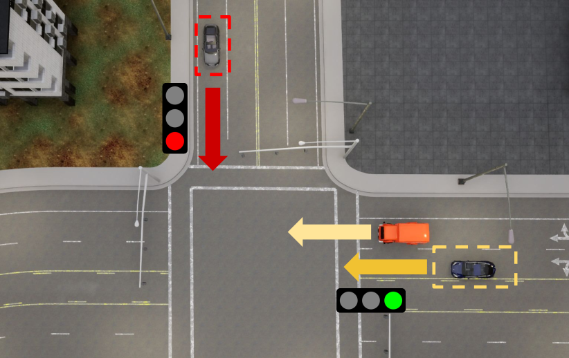
Figure 10. The orange truck obstructs the ego-vehicle’s (yellow box) view of red-light violator.

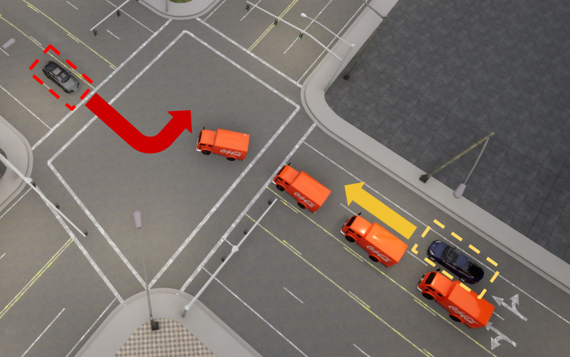
Figure 11. The orange trucks obstruct the ego-vehicle’s (yellow box) view of left-turning car.

NHTSA Scenario	Safe Passage (%)
	iDriving	Autonomous Driving
Red-light Violation	100	37
Unprotected Left-turn	100	18

Table 9. With more comprehensive perception, iDriving can provide safe passage to vehicles in both scenarios.

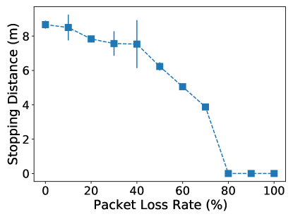
Figure 12. iDriving can ensure collision-free trajectories with up to 70% packet-loss rates.

Robustness to Packet Loss. iDriving’s planner transmits trajectories wirelessly to vehicles. It generates trajectories over a longer time horizon (§3) to be robust to packet loss. To quantify its robustness, we simulated packet losses ranging from 0 to 100% for in the red-light violation scenario (Fig. 11). For each loss rate, we measured the stopping distance between the ego-vehicle and the oncoming traffic which violates the red-light. Higher stopping distances are good (Fig. 12). We repeated the experiment multiple times for each loss rate. As we increased the packet-loss, the stopping distance decreased because the ego-vehicle was operating on increasingly stale information. Even so, iDriving ensures collision-free passage for the ego-vehicle through the intersection till 70% loss, with minimal degradation in stopping distance till about 40% loss.

4.6. High-Throughput Traffic Management

Intersections contribute significantly to traffic congestion [57]; traffic-light free intersections can reduce congestion and wait times. iDriving, because it centrally plans trajectories for all iDriving-capable vehicles, can plan collision-free trajectories at an intersection without traffic lights. We have verified this in simulations as well.

Wait-time Comparison. A traffic-light free intersection can significantly reduce wait times at intersections, thereby enabling higher throughput. To demonstrate this, we compared iDriving’s average wait times at an intersection against three other approaches:

Static

An intersection with static traffic lights.

Intelligent

Intelligent traffic light control which prioritizes longer queues.

Ideal-Coop

A traffic-light free intersection where autonomous vehicles use centralized perception but on-board decentralized planning. This represents an idealized version of cooperative perception like AVR [72], Autocast [73] and EMP [102] because it assumes that every vehicle has complete perception of all other traffic participants.

For the first two approaches, we obtained policies from published best practices [14, 20, 18]. In all experiments, we placed four LiDARs at an intersection in CarLA.

Results. Compared to Static and Intelligent, iDriving reduces average wait times for vehicles by up to 5$\times$ (Tbl. 10). iDriving performs better than even Intelligent because it can minimize the stop and start maneuvers at the intersection (by preemptively slowing down some vehicles), and hence can increase overall throughput, leading to lower wait times.

Interestingly, beyond about 6 vehicles, wait times for strategies that use traffic lights (Static and Intelligent) drops. Recall that our intersection has two lanes in each direction. As the number of vehicles increases, the probability that a vehicle can pass the intersection without waiting increases. For example, with Intelligent, a vehicle waiting at an intersection can trigger a green light, so a vehicle that arrives in the adjoining lane can pass without waiting. Even so, iDriving has lower wait times than other alternatives up to 10 vehicles (wait time comparisons are similar beyond this number, we omit results for brevity).

Tbl. 10 shows infinite wait times for Ideal-Coop. That is because, although one might expect that a decentralized planner might have comparable throughput to iDriving, we found that it led to a deadlock (§3) with as few as two vehicles (each vehicle waited indefinitely for the other to make progress, resulting in zero throughput). Fundamentally, this occurs because, with Ideal-Coop, vehicles lack global knowledge of planning decisions. Thus, deadlocks can happen at intersections without traffic lights even for more practical cooperative perception approaches which use on-board planners like AVR [72], Autocast [73], EMP [102].

Vehicle Count	Static	Intelligent	Ideal-Coop	iDriving
2	26.0	16.5	$\infty$	4.0
3	33.7	15.7	$\infty$	4.7
4	28.3	17	$\infty$	5.0
5	33.0	21.6	$\infty$	5.4
6	34.3	23.7	$\infty$	5.8
7	20.3	17.9	$\infty$	5.7
8	21.8	16.1	$\infty$	5.5
9	29.9	18.0	$\infty$	6.7
10	31.0	17.4	$\infty$	8.2

Table 10. iDriving minimizes average wait times (seconds) for vehicles with traffic light free intersections. Conventional traffic light strategies (Static and Intelligent) have more wait times due to start/stop maneuvers. Cooperative perception techniques (Ideal-Coop) can result in deadlocks ($\infty$ wait time) due to lack of global views.

5. Related Work

Connected Autonomous Vehicles. Network connectivity in vehicles has opened up large avenues for research; we cover these briefly. A large body of work [85] has explored wireless technologies and standards (such as DSRC) for vehicle-to-vehicle, and vehicle-to-infrastructure communication. Connected autononomous vehicles have also inspired proposals for cooperative perception [72, 102, 51], collaborative map updates [22], and cooperative driving [39, 61, 26] in which autonomous vehicles share information with each other to improve safety and utilization. Some have proposed approaches to offload route planning (but not trajectory planning) to the cloud [50]. Others explore is platooning [80, 56] in which vehicles collaboratively and dynamically form platoons to enable smooth traffic flows. Beyond inter-vehicle collaboration, several proposals have explored infrastructure support for connected autonomous vehicles, with infrastructure augmenting perception [75, 49], or delivering traffic light status [80]. Other work focuses on infrastructure-assisted traffic management at intersections [57]. iDriving goes beyond this body of work by demonstrating the feasibility of decoupling both perception and planning from vehicular control.

Infrastructure LiDAR based Perception. Prior work has explored using infrastructure LiDAR to detect pedestrians [103], and other road features such as lanes and drivable surfaces [96, 52], and to warn vehicles of impending collisions [25, 89]. One work [99] proposes a genetic algorithm based LiDAR alignment, but unlike iDriving, has not explored the efficacy of an entire perception pipeline built on top of LiDAR fusion.

Point Cloud Alignment. iDriving’s alignment builds upon point cloud registration techniques [29, 35, 81]. Prior work has matched features [78, 53] to align point clouds; these don’t work well for iDriving, where LiDARs capture the scene from very different perspectives.

Deep Neural Nets for 3D Detection and Tracking. Some work has developed neural nets for point-cloud based detection [104, 93, 58, 34, 98], and tracking [71, 48, 86, 30, 61, 62, 97]. These are too heavyweight for iDriving, and have been developed for vehicle-mounted LiDAR (iDriving exploits static LiDARs, §4.4).

Motion Estimation. Heading and velocity can be estimated using deep neural networks [62, 32], SLAM [64, 65, 42], or visual odometry [44, 94, 77]. iDriving uses a lightweight technique since it relies on static LiDARs.

6. Conclusions and Future Work

iDriving decouples autonomous vehicle perception and planning from low-level control. By doing this, it can perceive more than a single vehicle can, and jointly plan for multiple vehicles. To demonstrate that it can do this, while meeting the performance requirements of existing autonomous vehicles, and without sacrificing accuracy, we develop a novel stack containing new perception algorithms and a fast planner. Jointly, these achieve the desired performance targets on commodity hardware, and have accuracy comparable to state-of-the-art algorithms. At intersections, iDriving enables higher safety than autonomous driving, and higher throughput traffic management at intersections compared to using traffic lights.

Future work can seek to overcome some limitations in the current iDriving implementations.

• iDriving’s perception and planning modules are sensitive to the number of participants. To deal with this, future work can explore provisioning strategies which take historical traffic into account to provision edge compute to meet p99 latency goals. Alternatively, future work can also explore auto-scaling strategies: scaling-out edge compute when p99 latencies start to increase.

• iDriving’s perception and planning modules are relatively unoptimized; they execute perception and planning for every participant in every frame. It can avoid tracking and estimating heading for stationary vehicles and pedestrians (e.g., those waiting at the intersection). It can also avoid planning for such vehicles. Future work can explore these, and other optimizations (parallelizing tracking and heading estimation).

• Beyond intersections, iDriving can, in theory, enable a future world without autonomous driving; cars would not have on-board perception and planning, but would simply follow iDriving-generated trajectories. This can eliminate the need for expensive sensors [5, 76], power-hungry on-board compute [59], and expensive high-definition maps [87]. To achieve this vision, infrastructure needs to be installed everywhere, which will require much work: cost/benefit economic analyses, public-private partnerships to install infrastructure, regulatory approvals, buy-in from vehicle owners etc.

References

- [1] An Open Source Self-Driving Car.
- [2] Google Maps.
- [3] Vehicle stopping distance and time. https://nacto.org/docs/usdg/vehicle_stopping_distance_and_time_upenn.pdf.
- [4] Find minimum oriented bounding box of point cloud. http://codextechnicanum.blogspot.com/2015/04/find-minimum-oriented-bounding-box-of.html, 2015.
- [5] What it really costs to turn a car into a self-driving vehicle. https://qz.com/924212/what-it-really-costs-to-turn-a-car-into-a-self-driving-vehicle/, 2017.
- [6] Lidar sensors for combined smart city and av ecosystem. https://www.traffictechnologytoday.com/news/smart-cities/lidar-sensors-for-combined-smart-city-and-av-ecosystem.html, 2019.
- [7] The top five applications for lidar beyond the automotive market. https://enterpriseiotinsights.com/20191113/channels/opinion/five-applications-lidar-beyond-automotive-reader-forum, 2019.
- [8] Victoria to install lidar at high-crash intersections. https://www.itnews.com.au/news/victoria-to-install-lidar-at-high-crash-intersections-530967, 2019.
- [9] Ericsson 5G. https://www.ericsson.com/en/5g, 2020.
- [10] Exclusive: Huawei’s lidar is on the car, the price may be as low as hundreds of dollars. https://ycnews.com/exclusive-huaweis-lidar-is-on-the-car-the-price-may-be-as-low-as-hundreds-of-dollars/, 2020.
- [11] Introducing 5G Technology and Networks. https://www.thalesgroup.com/en/markets/digital-identity-and-security/mobile/inspired/5G, 2020.
- [12] Qualcomm 5G. https://www.qualcomm.com/invention/5g, 2020.
- [13] What is Edge Computing. https://www.ibm.com/cloud/what-is-edge-computing, 2020.
- [14] Automatically generated tls-programs. Traffic Lights - SUMO Documentation, 2021.
- [15] Baidu apollo specifications. https://github.com/ApolloAuto/apollo/blob/master/docs/specs/README.md, 2021.
- [16] Lane, Nov 2021.
- [17] Los angeles county home to state’s worst intersections: Report. Patch, 2021.
- [18] Signal cycle lengths. National Association of City Transportation Officials, 2021.
- [19] Statistics on intersection accidents. Federal Highway Administration, 2021.
- [20] Traffic signal timing manual, 2021. Chapter 5 - Office of Operations.
- [21] US Department of Transportation Federal Highway Administration - Intersection Safety, Jan 2022.
- [22] Fawad Ahmad, Hang Qiu, Ray Eells, Fan Bai, and Ramesh Govindan. Carmap: Fast 3d feature map updates for automobiles. In 17th USENIX Symposium on Networked Systems Design and Implementation (NSDI 20), pages 1063–1081, 2020.
- [23] Andrej Karpathy. CVPR’21 Workshop on Autonomous Driving: Andrej Karpathy Keynote.
- [24] Anton Andreychuk, Konstantin Yakovlev, Eli Boyarski, and Roni Stern. Improving continuous-time conflict based search, 2021.
- [25] Olivier Aycard. Intersection Safety Using Lidar and Stereo Vision Sensors on a Demonstrator Vehicle. Transportation, (IV):863–869, 2011.
- [26] Alessandro Bazzi, Barbara M Masini, Alberto Zanella, and Ilaria Thibault. On the performance of ieee 802.11 p and lte-v2v for the cooperative awareness of connected vehicles. IEEE Transactions on Vehicular Technology, 66(11):10419–10432, 2017.
- [27] Ben Bellekens, Vincent Spruyt, Rafael Berkvens, Rudi Penne, and Maarten Weyn. A benchmark survey of rigid 3d point cloud registration algorithms. Int. J. Adv. Intell. Syst, 8:118–127, 2015.
- [28] Keni Bernardin and Rainer Stiefelhagen. Evaluating multiple object tracking performance: the clear mot metrics. EURASIP Journal on Image and Video Processing, 2008:1–10, 2008.
- [29] P. J. Besl and N. D. McKay. A method for registration of 3-d shapes. IEEE Transactions on Pattern Analysis and Machine Intelligence, 14(2):239–256, 1992.
- [30] Adel Bibi, Tianzhu Zhang, and Bernard Ghanem. 3d part-based sparse tracker with automatic synchronization and registration. In Proceedings of the IEEE Conference on Computer Vision and Pattern Recognition, pages 1439–1448, 2016.
- [31] CarLA. Carla autonomous driving challenge, 2019.
- [32] Sergio Casas, Wenjie Luo, and Raquel Urtasun. IntentNet: Learning to Predict Intention from Raw Sensor Data. In Aude Billard, Anca Dragan, Jan Peters, and Jun Morimoto, editors, Proceedings of The 2nd Conference on Robot Learning, volume 87 of Proceedings of Machine Learning Research, pages 947–956. PMLR, 2018.
- [33] C.e.h. Average car length - list of car lengths in details - a new way forward: Automotive and home advice & review, Nov 2020.
- [34] Xiaozhi Chen, Huimin Ma, Ji Wan, Bo Li, and Tian Xia. Multi-view 3d object detection network for autonomous driving. In Proceedings of the IEEE Conference on Computer Vision and Pattern Recognition (CVPR), July 2017.
- [35] Y. Chen and G. Medioni. Object modeling by registration of multiple range images. In Proceedings. 1991 IEEE International Conference on Robotics and Automation, pages 2724–2729 vol.3, 1991.
- [36] Yang Chen and Gérard G. Medioni. Object modeling by registration of multiple range images. In Proceedings of the 1991 IEEE International Conference on Robotics and Automation, Sacramento, CA, USA, 9-11 April 1991, pages 2724–2729, 1991.
- [37] Zhe Chen, Jing Zhang, and Dacheng Tao. Progressive lidar adaptation for road detection. IEEE/CAA Journal of Automatica Sinica, 6(3):693–702, 2019.
- [38] Travelers Risk Control. 3-second rule for safe following distance.
- [39] Reza Dariani and Julian Schindler. Cooperative strategical decision and trajectory planning for automated vehicle in urban areas. In 2019 IEEE International Conference on Vehicular Electronics and Safety (ICVES), pages 1–6. IEEE, 2019.
- [40] Konstantinos G Derpanis. Overview of the ransac algorithm. Image Rochester NY, 4(1):2–3, 2010.
- [41] Alexey Dosovitskiy, German Ros, Felipe Codevilla, Antonio Lopez, and Vladlen Koltun. Carla: An open urban driving simulator. arXiv preprint arXiv:1711.03938, 2017.
- [42] Jakob Engel, Jörg Stückler, and Daniel Cremers. Large-scale direct slam with stereo cameras. In 2015 IEEE/RSJ International Conference on Intelligent Robots and Systems (IROS), pages 1935–1942. IEEE, 2015.
- [43] Martin Ester, Hans-Peter Kriegel, Jörg Sander, Xiaowei Xu, et al. A density-based algorithm for discovering clusters in large spatial databases with noise. In Kdd, volume 96, pages 226–231, 1996.
- [44] Christian Forster, Zichao Zhang, Michael Gassner, Manuel Werlberger, and Davide Scaramuzza. Svo: Semidirect visual odometry for monocular and multicamera systems. IEEE Transactions on Robotics, 33(2):249–265, 2016.
- [45] Ming Gao, Xinlei Wang, Kui Wu, Andre Pradhana, Eftychios Sifakis, Cem Yuksel, and Chenfanfu Jiang. Gpu optimization of material point methods. ACM Transactions on Graphics (TOG), 37(6):1–12, 2018.
- [46] Vincent Garcia, Eric Debreuve, and Michel Barlaud. Fast k nearest neighbor search using gpu, 2008.
- [47] Andreas Geiger, Philip Lenz, Christoph Stiller, and Raquel Urtasun. Vision meets robotics: The kitti dataset. The International Journal of Robotics Research, 32(11):1231–1237, 2013.
- [48] Silvio Giancola, Jesus Zarzar, and Bernard Ghanem. Leveraging shape completion for 3d siamese tracking. In Proceedings of the IEEE/CVF Conference on Computer Vision and Pattern Recognition, pages 1359–1368, 2019.
- [49] Swaminathan Gopalswamy and Sivakumar Rathinam. Infrastructure enabled autonomy: A distributed intelligence architecture for autonomous vehicles. In 2018 IEEE Intelligent Vehicles Symposium, IV 2018, Changshu, Suzhou, China, June 26-30, 2018, pages 986–992, 2018.
- [50] Jacopo Guanetti, Yeojun Kim, and Francesco Borrelli. Control of connected and automated vehicles: State of the art and future challenges. Annual Reviews in Control, 45:18–40, 2018.
- [51] Yuze He, Li Ma, Zhehao Jiang, Yi Tang, and Guoliang Xing. Vi-eye: Semantic-based 3d point cloud registration for infrastructure-assisted autonomous driving. In Proceedings of the 27th Annual International Conference on Mobile Computing and Networking, MobiCom ’21, page 573–586, New York, NY, USA, 2021. Association for Computing Machinery.
- [52] Aharon Bar Hillel, Ronen Lerner, Dan Levi, and Guy Raz. Recent progress in road and lane detection: a survey. Machine vision and applications, 25(3):727–745, 2014.
- [53] D. Holz, A. E. Ichim, F. Tombari, R. B. Rusu, and S. Behnke. Registration with the point cloud library: A modular framework for aligning in 3-d. IEEE Robotics Automation Magazine, 22(4):110–124, 2015.
- [54] Hou-Ning Hu, Qi-Zhi Cai, Dequan Wang, Ji Lin, Min Sun, Philipp Krahenbuhl, Trevor Darrell, and Fisher Yu. Joint monocular 3d vehicle detection and tracking. In Proceedings of the IEEE/CVF International Conference on Computer Vision (ICCV), October 2019.
- [55] Alireza G Kashani, Michael J Olsen, Christopher E Parrish, and Nicholas Wilson. A review of lidar radiometric processing: From ad hoc intensity correction to rigorous radiometric calibration. Sensors, 15(11):28099–28128, 2015.
- [56] Pooja Kavathekar and YangQuan Chen. Vehicle platooning: A brief survey and categorization. In ASME 2011 International Design Engineering Technical Conferences and Computers and Information in Engineering Conference, pages 829–845. American Society of Mechanical Engineers Digital Collection, 2011.
- [57] Mohammad Khayatian, Mohammadreza Mehrabian, Edward Andert, Rachel Dedinsky, Sarthake Choudhary, Yingyan Lou, and Aviral Shirvastava. A survey on intersection management of connected autonomous vehicles. ACM Trans. Cyber-Phys. Syst., 4(4), August 2020.
- [58] Bo Li. 3d fully convolutional network for vehicle detection in point cloud. In 2017 IEEE/RSJ International Conference on Intelligent Robots and Systems (IROS), pages 1513–1518. IEEE, 2017.
- [59] Shih-Chieh Lin, Yunqi Zhang, Chang-Hong Hsu, Matt Skach, Md. Enamul Haque, Lingjia Tang, and Jason Mars. The architectural implications of autonomous driving: Constraints and acceleration. In Proceedings of the Twenty-Third International Conference on Architectural Support for Programming Languages and Operating Systems, ASPLOS 2018, Williamsburg, VA, USA, March 24-28, 2018, pages 751–766, 2018.
- [60] T. Litman. Autonomous vehicle implementation predictions: Implications for transport planning, 2015.
- [61] Ye Liu, Xiao-Yuan Jing, Jianhui Nie, Hao Gao, Jun Liu, and Guo-Ping Jiang. Context-aware three-dimensional mean-shift with occlusion handling for robust object tracking in rgb-d videos. IEEE Transactions on Multimedia, 21(3):664–677, 2018.
- [62] Wenjie Luo, Bin Yang, and Raquel Urtasun. Fast and Furious: Real Time End-to-End 3D Detection, Tracking and Motion Forecasting With a Single Convolutional Net. In Proceedings of the IEEE Conference on Computer Vision and Pattern Recognition (CVPR), jun 2018.
- [63] Keita Miura, Shota Tokunaga, Noriyuki Ota, Yoshiharu Tange, and Takuya Azumi. Autoware toolbox: Matlab/simulink benchmark suite for ros-based self-driving software platform. In Proceedings of the 30th International Workshop on Rapid System Prototyping (RSP’19), RSP ’19, page 8–14, New York, NY, USA, 2019. Association for Computing Machinery.
- [64] Raul Mur-Artal, Jose Maria Martinez Montiel, and Juan D Tardos. Orb-slam: a versatile and accurate monocular slam system. IEEE transactions on robotics, 31(5):1147–1163, 2015.
- [65] Raul Mur-Artal and Juan D Tardós. Orb-slam2: An open-source slam system for monocular, stereo, and rgb-d cameras. IEEE Transactions on Robotics, 33(5):1255–1262, 2017.
- [66] Wassim G Najm, Raja Ranganathan, Gowrishankar Srinivasan, John D Smith, Samuel Toma, Elizabeth Swanson, August Burgett, et al. Description of light-vehicle pre-crash scenarios for safety applications based on vehicle-to-vehicle communications. Technical report, United States. National Highway Traffic Safety Administration, 2013.
- [67] Ouster. Ouster LiDAR. https://ouster.com/, 2020.
- [68] Brian Paden, Michal Cap, Sze Zheng Yong, Dmitry Yershov, and Emilio Frazzoli. A survey of motion planning and control techniques for self-driving urban vehicles. IEEE Transactions on intelligent vehicles, 1(1):33–55, 2016.
- [69] Scott Drew Pendleton, Hans Andersen, Xinxin Du, Xiaotong Shen, Malika Meghjani, You Hong Eng, Daniela Rus, and Marcelo H Ang. Perception, planning, control, and coordination for autonomous vehicles. Machines, 5(1):6, 2017.
- [70] Mike Phillips and Maxim Likhachev. Sipp: Safe interval path planning for dynamic environments. In 2011 IEEE International Conference on Robotics and Automation, pages 5628–5635. IEEE, 2011.
- [71] Haozhe Qi, Chen Feng, Zhiguo Cao, Feng Zhao, and Yang Xiao. P2b: Point-to-box network for 3d object tracking in point clouds. In Proceedings of the IEEE/CVF Conference on Computer Vision and Pattern Recognition (CVPR), June 2020.
- [72] Hang Qiu, Fawad Ahmad, Fan Bai, Marco Gruteser, and Ramesh Govindan. Avr: Augmented vehicular reality. In Proceedings of the 16th Annual International Conference on Mobile Systems, Applications, and Services, pages 81–95, 2018.
- [73] Hang Qiu, Pohan Huang, Namo Asavisanu, Xiaochen Liu, Konstantinos Psounis, and Ramesh Govindan. Autocast: Scalable infrastructure-less cooperative perception for distributed collaborative driving. In Proceedings of the 20th Annual International Conference on Mobile Systems, Applications, and Services, MobiSys ’22, 2022.
- [74] Morgan Quigley, Ken Conley, Brian Gerkey, Josh Faust, Tully Foote, Jeremy Leibs, Rob Wheeler, and Andrew Y Ng. Ros: an open-source robot operating system. In ICRA workshop on open source software, volume 3, page 5. Kobe, Japan, 2009.
- [75] Deepika Ravipati, Kenny Chour, Abhishek Nayak, Tyler Marr, Sheelabhadra Dey, Alvika Gautam, Sivakumar Rathinam, and Swaminathan Gopalswamy. Vision based localization for infrastructure enabled autonomy. In 2019 IEEE Intelligent Transportation Systems Conference, ITSC 2019, Auckland, New Zealand, October 27-30, 2019, pages 1638–1643, 2019.
- [76] Reuters. Self-driving costs could drop 90 percent by 2025, Delphi CEO says. https://www.reuters.com/article/us-autos-delphi/self-driving-costs-could-drop-90-percent-by-2025-delphi-ceo-says-idUSKBN1DY2AC, December 2017.
- [77] Antoni Rosinol, Marcus Abate, Yun Chang, and Luca Carlone. Kimera: an open-source library for real-time metric-semantic localization and mapping. In 2020 IEEE International Conference on Robotics and Automation (ICRA), pages 1689–1696. IEEE, 2020.
- [78] R. B. Rusu, N. Blodow, Z. C. Marton, and M. Beetz. Aligning point cloud views using persistent feature histograms. In 2008 IEEE/RSJ International Conference on Intelligent Robots and Systems, pages 3384–3391, 2008.
- [79] Radu Bogdan Rusu, Nico Blodow, and Michael Beetz. Fast point feature histograms (FPFH) for 3d registration. In 2009 IEEE International Conference on Robotics and Automation, ICRA 2009, Kobe, Japan, May 12-17, 2009, pages 3212–3217, 2009.
- [80] Julian Schindler, Reza Dariani, Michele Rondinone, and Thomas Walter. Dynamic and flexible platooning in urban areas. 2018.
- [81] Aleksandr Segal, Dirk Haehnel, and Sebastian Thrun. Generalized-icp. In Robotics: science and systems, volume 2, page 435. Seattle, WA, 2009.
- [82] Shai Shalev-Shwartz, Shaked Shammah, and Amnon Shashua. Safe, multi-agent, reinforcement learning for autonomous driving. arXiv preprint arXiv:1610.03295, 2016.
- [83] Shai Shalev-Shwartz, Shaked Shammah, and Amnon Shashua. On a formal model of safe and scalable self-driving cars, 2018.
- [84] Guni Sharon, Roni Stern, Ariel Felner, and Nathan R Sturtevant. Conflict-based search for optimal multi-agent pathfinding. Artificial Intelligence, 219:40–66, 2015.
- [85] J. E. Siegel, D. C. Erb, and S. E. Sarma. A survey of the connected vehicle landscape—architectures, enabling technologies, applications, and development areas. IEEE Transactions on Intelligent Transportation Systems, 19(8):2391–2406, 2018.
- [86] Shuran Song and Jianxiong Xiao. Tracking revisited using rgbd camera: Unified benchmark and baselines. In Proceedings of the IEEE international conference on computer vision, pages 233–240, 2013.
- [87] Synced. The Golden Age of HD Mapping for Autonomous Driving. https://medium.com/syncedreview/the-golden-age-of-hd-mapping-for-autonomous-driving-b2a2ec4c11d, August 2018.
- [88] Remi Tachet, Paolo Santi, Stanislav Sobolevsky, Luis Reyes-Castro, Emilio Frazzoli, Dirk Helbing, and Carlo Ratti. Revisiting street intersections using slot-based systems. PLOS ONE, 11:e0149607, 03 2016.
- [89] Andrew Tarko, Kartik Ariyur, Mario Romero, Vamsi Bandaru, and Cristhian Lizarazo. T-Scan: Stationary LiDAR for Traffic and Safety Applications—Vehicle Detection and Tracking. Number March. 2017.
- [90] Digital Trends. A Self-Driving Car in Every Driveway? Solid-State Lidar is the Key. https://www.digitaltrends.com/cars/solid-state-lidar-for-self-driving-cars/, 2018.
- [91] Shinji Umeyama. Least-squares estimation of transformation parameters between two point patterns. IEEE Computer Architecture Letters, 13(04):376–380, 1991.
- [92] Victor Vaquero, Ivan del Pino, Francese Moreno-Noguer, Joan Sola, Alberto Sanfeliu, and Juan Andrade-Cetto. Deconvolutional networks for point-cloud vehicle detection and tracking in driving scenarios. In 2017 European Conference on Mobile Robots (ECMR), pages 1–7. IEEE, 2017.
- [93] Dominic Zeng Wang and Ingmar Posner. Voting for voting in online point cloud object detection. In Robotics: Science and Systems, volume 1, pages 10–15607. Rome, Italy, 2015.
- [94] Rui Wang, Martin Schworer, and Daniel Cremers. Stereo dso: Large-scale direct sparse visual odometry with stereo cameras. In Proceedings of the IEEE International Conference on Computer Vision, pages 3903–3911, 2017.
- [95] Whoenig. Library with Search Algorithms for Task and Path Planning for Multi Robot/Agent Systems.
- [96] J Wu, H Xu, and J Zheng. Automatic background filtering and lane identification with roadside LiDAR data. In 2017 IEEE 20th International Conference on Intelligent Transportation Systems (ITSC), pages 1–6, oct 2017.
- [97] Bin Yang, Wenjie Luo, and Raquel Urtasun. Pixor: Real-time 3d object detection from point clouds. In Proceedings of the IEEE conference on Computer Vision and Pattern Recognition, pages 7652–7660, 2018.
- [98] Zetong Yang, Yanan Sun, Shu Liu, Xiaoyong Shen, and Jiaya Jia. Std: Sparse-to-dense 3d object detector for point cloud. In Proceedings of the IEEE/CVF International Conference on Computer Vision (ICCV), October 2019.
- [99] Rui Yue, Hao Xu, Jianqing Wu, Renjuan Sun, and Changwei Yuan. Data registration with ground points for roadside LiDAR sensors. Remote Sensing, 11(11), 2019.
- [100] Ji Zhang and Sanjiv Singh. Loam: Lidar odometry and mapping in real-time. In Robotics: Science and Systems, volume 2, 2014.
- [101] Ji Zhang and Sanjiv Singh. Visual-lidar odometry and mapping: Low-drift, robust, and fast. In 2015 IEEE International Conference on Robotics and Automation (ICRA), pages 2174–2181. IEEE, 2015.
- [102] Xumiao Zhang, Anlan Zhang, Jiachen Sun, Xiao Zhu, Y Ethan Guo, Feng Qian, and Z Morley Mao. Emp: edge-assisted multi-vehicle perception. In Proceedings of the 27th Annual International Conference on Mobile Computing and Networking, pages 545–558, 2021.
- [103] Junxuan Zhao, Hao Xu, Hongchao Liu, Jianqing Wu, Yichen Zheng, and Dayong Wu. Detection and tracking of pedestrians and vehicles using roadside LiDAR sensors. Transportation Research Part C: Emerging Technologies, 100(December 2017):68–87, 2019.
- [104] Yin Zhou and Oncel Tuzel. Voxelnet: End-to-end learning for point cloud based 3d object detection. In Proceedings of the IEEE Conference on Computer Vision and Pattern Recognition (CVPR), June 2018.