Low frequency radio continuum imaging and SED modeling of 11 LIRGs: radio-only and FUV to radio bands

Abstract

We present the detailed analysis of 11 local luminous infrared galaxies (LIRGs) from ultraviolet through far-infrared to radio ($\sim$70  MHz to $\sim$15 GHz) bands. We derive the astrophysical properties through spectral energy distribution (SED) modeling using the Code Investigating GALaxy Emission (CIGALE) and UltraNest codes. The radio SEDs include our new observations at 325 and 610 MHz from the GMRT and the measurements from public archives. Our main results are (1) radio SEDs show turnovers and bends, (2) the synchrotron spectral index of the fitted radio spectra ranges between $-$0.5 and $-$1.7, and (3) the infrared luminosity, dust mass, dust temperature, stellar mass, star-formation rates (SFRs) and AGN fraction obtained from CIGALE falls in the range exhibited by galaxies of the same class. The ratio of 60$\mu$m infrared and 1.4 GHz radio luminosity, the 1.4 GHz thermal fraction, and emission measure range between 2.1 and 2.9, 0.1% and 10%, 0.02 and 269.5$\times$10${}^{6}$ cm${}^{-6}$ pc, respectively. We conclude that the turnovers seen in the radio SEDs are due to free-free absorption; this is supported by the low AGN fraction derived from the CIGALE analysis. The decomposed 1.4 GHz thermal and nonthermal radio luminosities allowed us to compute the star formation rate (SFR) using scaling relations. A positive correlation is observed between the SFR${}_{IR}$ obtained 10 Myr ago (compared to 100 Myr ago) and 1.4 GHz radio (total and nonthermal) because similar synchrotron lifetimes are expected for typical magnetic field strengths observed in these galaxies ($\approx$50$\mu$G).

1 Introduction

Table 1: Basic information on our sample of LIRGs

Name	R.A.(J2000)	Dec.(J2000)	$z$	log${}_{10}$($L_{IR}$)
	(h m s)	(${}^{\circ}$ ${}^{\prime}$ $\arcsec$)		($L_{\odot}$)
(1)	(2)	(3)	(4)	(5)
ESO 500-G034	10 24 31.4	$-$23 33 10	0.0122	10.77
NGC 3508	11 02 59.7	$-$16 17 22	0.0128	10.65
ESO 440-IG058	12 06 51.9	$-$31 56 54	0.0232	11.18
ESO 507-G070	13 02 52.3	$-$23 55 18	0.0217	11.34
NGC 5135	13 25 44.0	$-$29 50 01	0.0136	11.12
IC 4280	13 32 53.4	$-$24 12 26	0.0162	10.85
NGC 6000	15 49 49.6	$-$29 23 13	0.0070	10.92
IR 16164-0746	16 19 11.8	$-$07 54 03	0.0271	11.29
ESO 453-G005	16 47 31.1	$-$29 21 22	0.0209	11.69
IR 18293-3413	18 32 41.1	$-$34 11 27	0.0181	11.62
ESO 593-IG008	19 14 31.1	$-$21 19 09	0.0485	11.77

Columns : (1) source name, (2) right ascension, (3) declination, (4) spectroscopic redshift from the NASA/IPAC Extragalactic Database (NED); (5) absolute far-$IR$ luminosity from Table 1 of Condon et al. (1996), except for NGC 3508 which is taken from Table 1 of Condon et al. (1990).

Characterized by a prodigious amount of emission at infrared ($IR$) wavebands, luminous and ultra-luminous infrared galaxies ((U)LIRGs) dominate the infrared sky. LIRGs and ULIRGs have infrared luminosity in the wavelength range 8$\mu$m $<$ $\lambda$ $<$ 1000$\mu$m, $L_{IR}$, $\sim>10^{11}$ $L_{\odot}$ and $\sim>10^{12}$ $L_{\odot}$, respectively, where $L_{\odot}$ is the solar luminosity (Helou et al., 1988). As the name suggests, these galaxies bridge the gap between underlying astrophysical processes contributing to emission in normal star-forming galaxies and the active galactic nuclei (AGN) activity (see, for a review Sanders & Mirabel, 1996; Pérez-Torres et al., 2021). Their spectral energy distribution (SED), although dominated by emission at infrared wavebands, ranges from radio to UV/X-rays frequencies (Yun et al., 2001; Pereira-Santaella et al., 2011), containing imprints of different astrophysical processes such as star formation, stellar evolution, chemical enrichment, processes in the interstellar medium, and the AGN (e.g., Conroy, 2013). Therefore, a detailed and broadband SED modeling provides not only important constraints on astrophysical properties shaping SEDs, but also the evolutionary history of a galaxy, providing insights into the cosmic evolution of the galaxy population (Lonsdale et al., 2006).

As the radio waves remain unaffected by dust, the study of the radio continuum offers a promising approach for studying the astrophysical properties of galaxies. The q${}_{IR}$ parameter, defined as the ratio of infrared (60-100 $\mu$m) to radio (1.4 GHz) luminosities, shows a surprisingly tight correlation for normal galaxies because emission at these wavebands is ascribed to a common origin and interpreted as calorimetric models (Helou et al., 1988; Condon, 1992; Yun et al., 2001; Murphy, 2009). In this framework, the galaxies are optically thick to UV radiation from young massive stars that are absorbed by the dust in the interstellar medium and reradiated in the far-infrared (FIR) regime. Later on, these stars explode to form type II supernovae and accelerate cosmic-ray electron (CRe) that produces radio emission via a synchrotron process before escaping the galaxy (Voelk, 1989). Helou et al. (1985) suggested that galaxies can be optically thin to both UV photons and cosmic rays, but coupling between gas and magnetic field should exist to maintain the radio-IR correlation (see also, Lacki et al., 2010; Tabatabaei et al., 2013). Furthermore, a secondary component of the radio continuum emission due to free-free interactions between charged particles, i.e., free-free radiation, is also produced by ionization of gas in H${}_{\textsc{II}}$ regions. In general, synchrotron emission is characterized by a power-law emission spectrum, $f_{\nu}\,\propto\nu^{\alpha}$ $(\alpha\simeq-0.8)$ dominating the 1–10 GHz frequency range, whereas free-free emission has almost a flat spectrum with flux proportional to $\nu^{-0.1}$, dominating in frequency range $\geq$ 10 GHz (Condon, 1992). The radio spectra of galaxies bend (or flatten) at lower frequencies $<$1GHz due to absorption processes such as free-free absorption (FFA), synchrotron self-absorption (SSA) or the Tsytovitch-Razin effect (Israel & Mahoney, 1990; Condon, 1992; Clemens et al., 2010; Marvil et al., 2015).

Therefore, the exact shape of the radio spectra between the MHz to GHz range depends on either the quantity and distribution of ionized (thermal) gas in galaxies (Vardoulaki et al., 2015; Clemens et al., 2008; Chyży et al., 2018; Galvin et al., 2018) or due to the presence of the AGN (Clemens et al., 2010). Typically, the thermal fraction, $TF$, defined as the ratio of thermal to total emission, ranges between 0.1 and 10% at 1.4 GHz for normal star-forming galaxies and LIRGs (see, Galvin et al., 2018). Therefore, constraining the radio spectrum to low frequencies is essential to understand the absorption models for these galaxies.

Multiwavelength SED modeling, from ultraviolet (UV) to IR, provides information about the light emitted by stars, either directly or through reprocessing by the gas (emission and absorption features in the SED) and dust in the interstellar medium, while radio SED probes the nonthermal and thermal processes in galaxies (see, for a review, Walcher et al., 2011; Tabatabaei et al., 2017; Pérez-Torres et al., 2021). Therefore, different regimes of the broad SED provide critical insight into the nature, origin of emission, and factors that establish the energy balance. The astrophysical properties of galaxies using the Code Investigating GALaxy Emission (CIGALE) model set for main-sequence (normal) star-forming galaxies (Ciesla et al., 2017; Vika et al., 2017; Pearson et al., 2018; Riccio et al., 2021; Shirley et al., 2021), LIRGs, and ULIRGs have been characterized (Małek et al., 2017, 2018; Paspaliaris et al., 2021). As these galaxies can host AGNs, the CIGALE code includes the AGN component in the modeling. In particular, the AGN fraction (defined as the ratio of $IR$ luminosity due to AGN and a sum of $IR$ luminosity due to AGN and starburst), stellar mass (M${}_{\star}$), star formation rate (SFR${}_{IR}$), dust luminosity ($L_{IR}$), dust temperature ($T_{\rm dust}$) have been obtained. The most significant finding of these studies is that LIRGs are characterized by a relatively higher SFR${}_{IR}$, $L_{IR}$, $T_{\rm dust}$, AGN fraction compared to normal star-forming galaxies and lower than those obtained by ULIRGs (Małek et al., 2017). On the other hand, detailed radio-SED analyses of a large sample of galaxies are rare, primarily due to the lack of wide-area multifrequency radio surveys and targeted follow-up of suitable samples.

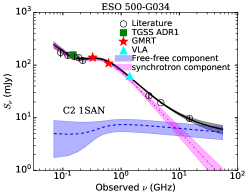
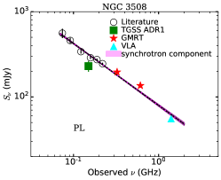
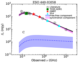
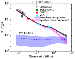
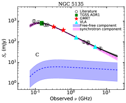
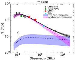
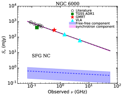
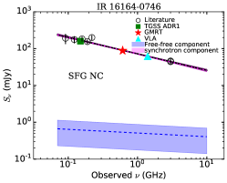
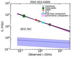
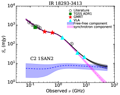
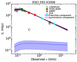
Figure 1: Radio SED for our sample of LIRGs. Galaxy name and the best-fit radio SED model name are given at the top and inside each panel. The solid black line represents the best-fit model, while the gray shaded region represents the 1$\sigma$ uncertainties sampled by the UltraNest package. The dot-dashed magenta and dotted blue lines show the decomposed synchrotron and free-free components. The pink and blue shaded regions represent the 1$\sigma$ uncertainties in the synchrotron and free-free components, respectively. For galaxies fitted with two-component models, the free-free and synchrotron components correspond to the sum of individual free-free and synchrotron components. The flux density measurements obtained with GMRT (365 and 610 MHz) are shown by the filled red star symbol, while the archival VLA data that were reduced and analyzed by us (1.4, 4.8, 8.4, and 14.9 GHz) are shown by the filled cyan triangle. The filled green square indicates the TGSS ADR1 150 MHz fluxes, and the open circle represents the flux density measurements taken from the literature (GLEAM, SUMSS, NVSS, VLASS, ATCA, and Effelsberg telescope) (see Section 3.1, Table A2).

With this motivation, we performed a SED modeling of radio-only and far-ultraviolet (FUV) to radio bands of a sample of 11 LIRGs, including our new measurements at 325 and 610 MHz frequencies using the Giant Metrewave Radio Telescope (GMRT; Swarup, 1990), operated by the National Centre of Radio Astronomy-Tata Institute of Fundamental Research, India. In this paper, we report the results of detailed radio SED modeling covering $\sim$80 MHz to $\sim$15 GHz and CIGALE SED modeling covering GHz band radio frequencies up to UV frequencies. As the CIGALE modeling cannot capture the complex shapes of low-frequency radio spectra exhibited by LIRGs and ULIRGs (e.g., Clemens et al., 2008, 2010; Galvin et al., 2018), therefore, we include $>$1.4 GHz band radio fluxes to cover the five decades of the spectral range. Furthermore, an essential aspect of CIGALE modeling is that it works on the energy balance between $UV$ and $IR$, which is ultimately related to the radio luminosity, hence including radio fluxes in CIGALE modeling is essential for better constraining the model parameter space (in particular, the $L_{\rm dust}$).

One of the primary goals of this paper is to compare the astrophysical properties resulting from SED modeling at radio-only and FUV to radio bands. The shapes of SEDs reflect the radiation laws and their parameters (such as power-law energy index or emissivity) and the physical processes affecting those parameters, such as cooling or heating mechanisms in the medium. Moreover, integrated SEDs provide total energetics from different frequency regimes, and comparing those offers key information on the nature of emission and general factors that determine their energy balance principle. Furthermore, our radio SED modeling allowed us to decompose the nonthermal and thermal emission components and estimate the star formation rate (SFR) using the basic nonthermal and thermal radio SFR calibration presented in Murphy et al. (2011) and compare them with the SFR${}_{IR}$ estimated from CIGALE SED modeling.

We perform detailed SED modeling of a sample of 11 nearby LIRGs (median redshift equal to 0.0181), focusing separately on radio-only and FUV-radio spectral bands. The paper is organized as follows. Sample selection is given in Section 2 while Section 3 describes data collection and analysis. Section 4 gives details of the radio-only and panchromatic (FUV to radio) SED modeling procedures. Section 5 gives the results of model fitting, i.e., characterization of astrophysical properties of our sample. The discussion of the results obtained is given in Section 6 while the conclusion is given in Section 7.

2 sample selection

In this study, we have assembled a sample of 10 LIRGs with the selection criteria log${}_{10}(L_{IR})$ $>$ 10.75 $L_{\odot}$ from the 1.425 GHz Atlas of the IRAS Bright Galaxy Sample catalog (Condon et al., 1996) and one galaxy, NGC 3508 from the 1.49 GHz Atlas of the IRAS Bright Galaxy Sample (Condon et al., 1990) of with flux densities greater than 5.24 Jy at 60$\mu$m. These galaxies were selected based on the availability of 150 MHz data in the original release of the TIFR GMRT Sky Survey (TGSS) Data Release (DR) 4, covering 1 sr of the sky, using the GMRT (see, for a basic description of the survey; Sirothia et al., 2014). We note that Intema et al. (2017) presented the entire TGSS data in their alternate data release (TGSS ADR1). Although, we selected our sample from the original TGSS DR 4 release, which had slightly better sensitivity for extended emission (rms error $\sim$7-9 mJy beam${}^{-1}$) as compared to the TGSS ADR1 (Intema et al., 2017), we use TGSS ADR1 integrated fluxes for radio SED fitting as its reduction and calibration methodology is fully described. The basic properties of the LIRG sample are listed in Table 1.

Table 2: An overview of the natural log of the Bayes odds ratio from the UltraNest fitting of each model to each source. In boldface, we present the most preferred model with highest evidence value (see Eq. 10).

Name	PL	SFG	C	SFG	C2	C2	C2	C2
		NC		NC2	1SA	1SAN	1SAN2
ESO 500-G034	$-$68.1	$-$67.5	$-$6.3	$-$76.3	$-$1.2	0	$-$1.5	$-$4.2
NGC 3508	0	$-$3.5	$-$7.2	$-$8.7	$-$19.3	$-$4.6	$-$2.8	$-$7.1
ESO 440-IG058	$-$17.2	$-$14.9	0	$-$25.7	$-$3.9	$-$9.1	$-$6.8	$-$2.3
ESO 507-G070	$-$74.2	$-$69.9	$-$159.1	$-$21.8	$-$235.1	$-$1.9	0	$-$453.1
NGC 5135	$-$6.5	$-$3.7	0	$-$11.8	$-$13.0	$-$2.9	$-$35.4	$-$6.8
IC 4280	$-$3.2	$-$6.1	0	$-$12.4	$-$8.8	$-$1.6	$-$4.4	$-$0.7
NGC 6000	$-$3.4	0	$-$21.4	$-$6.1	$-$11.2	$-$1.6	$-$3.1	$-$408.8
IR 16164-0746	$-$3.4	0	$-$1.2	$-$1.3	$-$4.1	$-$0.9	$-$0.8	$-$3.0
ESO 453-G005	$-$2.9	0	$-$0.6	$-$3.5	$-$4.9	$-$2.1	$-$2.3	$-$1.5
IR 18293-3413	$-$88.7	$-$86.8	$-$90.4	$-$99.5	$-$4.3	$-$5.1	0	$-$5.1
ESO 593-IG008	$-$3.0	$-$5.9	0	$-$7.5	$-$4.3	$-$6.8	$-$3.8	$-$2.1

3 multi-wavelength datasets: Radio to FUV

3.1 Radio data and AIPS analysis

To construct the integrated radio SED for modeling, we use data in the $\sim$70 MHz to 15 GHz frequency range. These include our continuum observations at 325 and 610 MHz conducted using the GMRT (ID: 23_051, PI: Arti Goyal) and the publicly available archival datasets at 4.8, 8.4, and 14.5 GHz from the Karl G. Jansky Very Large Array (VLA), operated by the National Radio Astronomical Observatory, USA.

3.1.1 New GMRT data at 325 and 610 MHz

We carried out radio continuum imaging of our sample using the GMRT at 325 MHz and 610 MHz. The primary and phase calibrators used in our observations are provided in Table A1. We observed each target with 32 MHz bandwidth divided into 256 spectral channels. We observed standard flux calibrators at the beginning and end of the observation to calibrate the antenna gains. Phase calibrators were selected from the NRAO VLA calibrator manual list and were within 20 deg. Phase calibrators were observed every 30 minutes for a typical duration of 4-5 minutes to correct for antenna gain drifts, atmospheric and ionospheric gain, and phase variations. Each source was observed for a total duration of 32 minutes, in two scans consisting of 16 minutes each to enable better U-V coverage.

3.1.2 Archival VLA data at 1.4, 4.8, 8.4, and 14.9 GHz

We analyzed the archival VLA data for galaxies wherever possible. Most galaxies in our sample were observed for a few minutes of integration time with different array configurations and different central frequencies. The dataset with the largest on-source integration time was reduced when several observations were available with the same configuration and central frequency.

3.1.3 AIPS analysis

The interferometric observations from both the GMRT and the VLA were analyzed using NRAO AIPS. Data reduction was carried out in a standard fashion. The flux density scale of Baars et al. (1977) was used to obtain the flux densities of the primary (flux) calibrator, the secondary (phase) calibrator, and the target source. Antennas and baselines affected with strong radio frequency interference (RFI), nonworking antennas, were edited out after visual inspection. For the GMRT datasets, bandpass calibration was determined using the phase calibrator and the spectral channels were collapsed to generate the continuum database. Usually, spectral channels below ten and above 200 were discarded before collapsing the data. Images were produced using task imagr on the channel collapsed data. To correct for distortions in the imaging, the large field of view with noncoplanar baselines (GMRT at frequencies $<$1 GHz), polyhedron imaging was employed where the field of view was divided into smaller fields (facets). These were $5\times 5$ facets that covered the entire field of view up to the half power beam width (HPBW). Usually, 3-5 rounds of phase-based self-calibration were performed iteratively by choosing point sources in the field such that the flux density is $>$3$\sigma$ with one synthesized beam. The final images were made with full UV-coverage and robust weighting of 0 to weight the UV data (Briggs, 1995). Facets were combined using the task flatn. The same steps were followed for the VLA observations except that the data were obtained in two intermediate frequency (IF) channels calibrated for antenna gains before averaging them together for imaging. We did not apply any band-pass calibration since the data were obtained in a single spectral channel of 50 MHz bandwidth (BW). The final images were corrected for the reduction in sensitivity due to the shape of the antenna beam using task pbcor with the specified parameters for the GMRT and the VLA.

Integrated flux densities (and uncertainty) were obtained using the task TVSTAT in AIPS for the GMRT and VLA images. We note that the synthesized beam sizes range from $\sim$0.6-38${{}^{\prime\prime}}$. Assuming a typical resolution of 5${{}^{\prime\prime}}$, the linear scale is be 0.5–4 kpc at the galaxy distance ($z$ =  0.007–0.048). Therefore, it is reasonable to state that we obtain emissions from extended regions in most galaxies. Furthermore, we note in GMRT observations, all the proposed galaxies are detected at 610 MHz observations while LIRGs NGC 6000, IR 16164$-$0746 and ESO 453-G005 could not be detected at 325 MHz because the data could not be calibrated by weak phase calibrator.

3.1.4 Radio fluxes from the literature

We searched for flux measurements at other frequencies along with the observations described above. In particular, we obtained measurements at the central frequencies of 74 MHz from the VLA Low-Frequency Sky Survey (VLSSr; Cohen et al., 2007), 74-231 MHz GaLactic, and Extragalactic MWA Survey (GLEAM; Wayth et al., 2015), 150 MHz TGSS ADR, 843 MHz Sydney University Molonglo Sky Survey (SUMSS; Mauch et al., 2003, 2013), 3.0 GHz VLA Sky Survey (VLASS; Lacy et al., 2020; Gordon et al., 2021) within the positional uncertainties provided by the survey parameters. For LIRGs ESO440-IG080 and ESO500-G034, we also included 10.0 GHz flux densities from the Australia Telescope Compact Array, published in Hill et al. (2001). For NGC 5135, we included 2.3 GHz measurements from the $S-$band Polarization All-Sky Survey (Meyers et al., 2017), and 6.7 GHz measurements from the Effelsburg telescope (Impellizzeri et al., 2008). In addition, we also included 1.4 GHz NRAO VLA Sky Survey (NVSS; Condon et al., 1998) flux for the galaxy IR 18293$-$3413. The GLEAM survey frequency bands are 72-103 MHz, 103-134 MHz, 139-170 MHz, 170-200 MHz, and 200-231 MHz where each band is divided into 7.68 MHz sub-channels for imaging purposes (Hurley-Walker et al., 2017). The survey provides flux measurements into subbands of 7.68 MHz BW (each band has a frequency resolution of 30.72 MHz), which are not independent of each other; therefore, we averaged the fluxes within each band for spectral modeling.

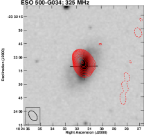
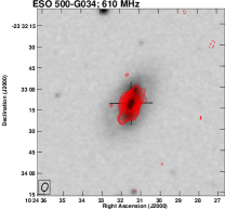
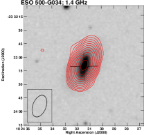
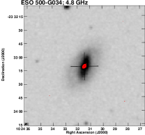
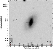
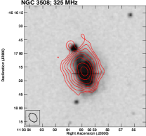
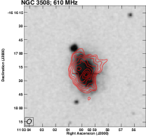
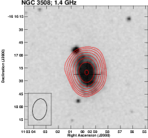
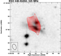
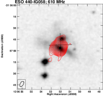
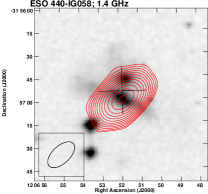
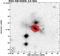
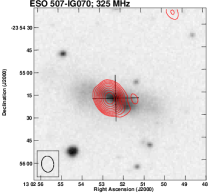
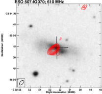
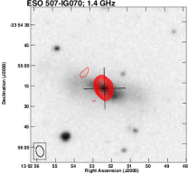
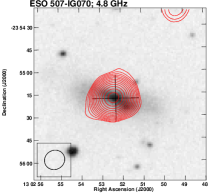
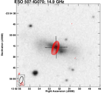
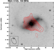
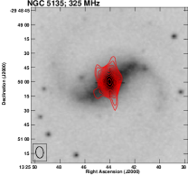
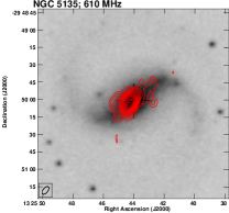
Figure 14: 150 MHz-15 GHz radio contour images (red) overlaid on the optical DSS2 R-band images (grey scale) for the samples of 11 LIRGs analysed by us. The radio contours begin at 3$\sigma$ of the rms noise on the radio map (Column 8 of Tab. A2) and increase by $(\sqrt{2})^{n}$ where $n$ ranges from 0,1,2,..20. The -3$\sigma$ radio intensity is shown by dashed contours and the synthesized beam achieved is given at the bottom left corner of the image.

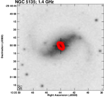
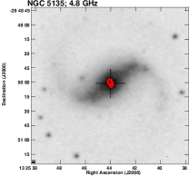
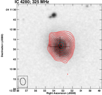
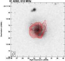
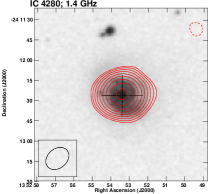
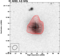
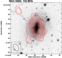
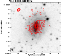
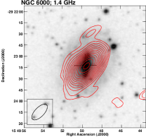
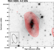
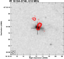
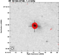
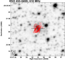
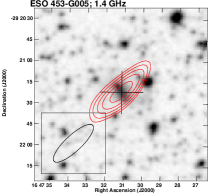
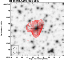
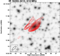
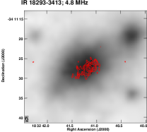
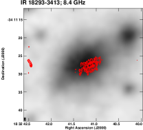
Figure 14: continued

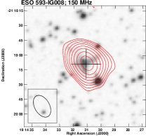
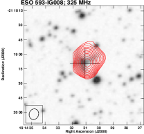
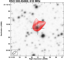
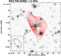
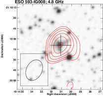
Figure 14: continued

Table A2 summarizes the GMRT and VLA datasets analyzed by us, while Figure 14 provides total intensity radio maps overlaid on Digital Sky Survey (DSS)2-$R$-band images in Appendix A. For radio SED modeling, we further upscaled the errors to account for variations in uncalibrated system temperature. In particular, we added in quadrature to the flux density errors an additional 10% for 150 MHz TGSS ADR1 (Intema et al., 2017), 5% for 325 and 610 MHz GMRT (Żywucka et al., 2014; Mhlahlo & Jamrozy, 2021), 3% for 1.4, 4.8, 8.4, and 14.9 GHz VLA (Perley & Butler, 2017), 3% for NVSS (Condon et al., 1998), 10% for VLASS (Lacy et al., 2020), 10% for GLEAM (Mhlahlo & Jamrozy, 2021), 5% for SUMSS (Mauch et al., 2003; Galvin et al., 2018), 15% for Effelsberg measurements (Impellizzeri et al., 2008), 10% for $S$-PASS (Meyers et al., 2017), and 5% for ATCA (Galvin et al., 2018) measurements, respectively, as calibration error (see Eq. 1 of Żywucka et al., 2014). As can be seen from Table A2 that the synthesized beam sizes for our continuum images range between a few arcseconds and 10$\times$ a few arcseconds. Because we analyzed datasets taken mostly at the B, C, and D array configurations of the VLA, it is unlikely that our galaxies are missing flux due to the lack of short U-V spacing data. To establish this, we compared the 1.4 GHz fluxes from Table A2 with the NVSS fluxes, obtained at a resolution of 45${}^{\arcsec}$. The two measurements are comparable within the measurement uncertainties. Table A3 provides the list of flux measurements used for the radio SED fitting.

3.2 UV, optical, and infrared fluxes

We collected photometric measurements from several instruments from both ground and space-based facilities for SED modeling using CIGALE. Specifically, we obtained the fluxes from the literature by cross-matching the optical positions of our galaxies to public databases such as NED (NASA/IPAC Extragalactic Database (2019), NED), SIMBAD (Wenger et al., 2000), VizieR (Ochsenbein, 1996), and NASA/IPAC Infrared Science Archive (IRSA) using a matching radius of 5${}^{\arcsec}$–15${}^{\arcsec}$. This matching radius was chosen to ensure that there exists a counterpart, depending on the instrument’s resolution. Specifically, the $UV$ and optical data were collected from the NED and VizieR Photometry viewer, while the infrared data were obtained from the IRSA database.

About 20–30 bands of $UV$–$IR$ broadband photometry are available for these sources. They include measurements from Galaxy Evolution Explorer (GALEX), Optical/UV monitor of XMM-Newton telescope (XMM-OM), Swift ultraviolet/optical telescope, SkyMapper Southern Sky Survey (SMSS), Sloan Digital Sky Survey (SDSS) DR 16, the Two-Micron All-Sky Survey (2MASS), the Wide-field Infrared Survey Explorer (WISE), Spitzer space telescope, AKARI, and Herschel Space Observatory. Table A4 gives the instrument characteristics. In the case of the availability of multiple flux measurements at a given wavelength, we chose the one that contained the entire galaxy. Moreover, five galaxies in our sample, namely, ESO 440-IG058, ESO 507-G070, ESO 593-IG008, IR 16164-0746, and IR 18293-3413 are either interacting, merging, or post-merging type; for these, the fluxes used in modeling include emission from the companion, too. Table LABEL:tab:UV-IRflux gives the integrated fluxes along with the integration area per band for each source used for SED modeling. For galaxies ESO 440-IG058 and NGC 5135, the IRAC apertures were optimized on a source by source basis to cover individual components when measuring galaxies in merger systems and to contain all the integrated flux in the case of isolated galaxies (Mazzarella et al., in preparation)

4 SED modeling

4.1 Radio SED

Integrated radio SEDs are modeled with physically motivated scenarios in which the radio continuum originates from either single or two emission regions characterized by the same or different populations of CRe and optical depths. Most of our adopted models are presented in Galvin et al. (2018). All modeling was performed in the observers’ frame with a reference frequency, $\nu_{0}$ = 1.4 GHz. We consider the following models:

4.1.1 Single power-law (PL)

A single power-law model with emission characterized by synchrotron processes, following the form:

$$S_{\nu}=A\left(\frac{\nu}{\nu_{0}}\right)^{\alpha}$$ (1)

where, A and $\alpha$ are the normalization and the spectral index, respectively, treated as free parameters.

4.1.2 Synchrotron and Free-Free Emission (SFG NC)

A radio continuum as a sum of optically thin (no curvature) synchrotron and free–free emission processes, following the form:

$$S_{\nu}=A\left(\frac{\nu}{\nu_{0}}\right)^{\alpha}+B\left(\frac{\nu}{\nu_{0}}\right)^{-0.1}$$ (2)

where A and B are the nonthermal and thermal normalization components, respectively, treated as free parameters. The free parameter, $\alpha$, is the synchrotron spectral index.

4.1.3 Synchrotron and Free-Free Emission with free-free absorption (C)

A radio continuum as a sum of optically thick synchrotron and free–free emission processes where the synchrotron emission can be suppressed due to FFA. If the frequency of this turnover due to FFA is parametrized by $\nu_{t,1}$ then the optical depth, $\tau$, can be defined as $(\nu/\nu_{t,1})^{-2.1}$. This model has the following form:

$$S_{\nu}=\left(1-e^{-\tau}\right)\left[B+A\left(\frac{\nu}{\nu_{t,1}}\right)^{0.1+\alpha}\right]\left(\frac{\nu}{\nu_{t,1}}\right)^{2}$$ (3)

where A and B are the nonthermal and thermal normalization components and treated as free parameters. The free parameters, $\nu_{t,1}$ and $\alpha$ are the turnover frequency and the synchrotron spectral index, respectively. To reduce the degeneracy of the model, we replace the term $\nu_{0}$ with the turnover frequency parameter for each component. A key point here is that the models assume that the synchrotron emission is completely commingled within extended plasma, which causes the free-free absorption (a plasma will exhibit FFA regardless of the physical origin of the radio photon - i.e. it does not matter what causes a radio photon to be there; it will get absorbed by the plasma).

4.1.4 Multiple Free-Free absorption (FFA) components

Multiple (two) components with emission and absorption representing two star-forming regions with different orientations or compositions. The radio continuum could be complex in these cases, as these regions are integrated by large synthesized beams for unresolved galaxies. We distinguish five scenarios in the multiple components framework which are described below:
(a) radio continuum originating from two different relativistic electron populations, characterized by synchrotron spectral indices, $\alpha$ and $\alpha_{2}$ in two distinct star-forming regions without FFA turnovers, labelled as SFG NC2, following the form:

$$S_{\nu}=A\left(\frac{\nu}{\nu_{0}}\right)^{\alpha}+B\left(\frac{\nu}{\nu_{0}}\right)^{-0.1}$$

$$+C\left(\frac{\nu}{\nu_{0}}\right)^{\alpha 2}+D\left(\frac{\nu}{\nu_{0}}\right)^{-0.1}$$ (4)

where, A and C are the nonthermal normalization components, respectively, while B and D are the thermal normalization components, respectively. A, B, C, D, $\alpha$, and $\alpha_{2}$ are treated as free parameters.

(b) radio continuum characterized by the same (single) relativistic electron population, $\alpha$, in two distinct star-forming regions having different optical depths, $\tau_{1}$ and $\tau_{2}$, respectively, labelled as “C2 1SA”:

$$S_{\nu}=\left(1-e^{-\tau_{1}}\right)\left[B+A\left(\frac{\nu}{\nu_{t,1}}\right)^{0.1+\alpha}\right]\left(\frac{\nu}{\nu_{t,1}}\right)^{2}$$

$$+\left(1-e^{-\tau_{2}}\right)\left[D+C\left(\frac{\nu}{\nu_{t,2}}\right)^{0.1+\alpha}\right]\left(\frac{\nu}{\nu_{t,2}}\right)^{2}$$ (5)

where, A and C are the nonthermal normalization components, respectively, while B and D are the thermal normalization components, respectively. A, B, C, D, $\alpha$, $\tau_{1}$ and $\tau_{2}$ are treated as free parameters.

(c) radio continuum characterized by the same (single) relativistic electron population, $\alpha$, in two distinct star-forming regions, one without a turnover (optically thin) while the other characterized by optical depth, $\tau_{2}$ (optically thick), respectively, labelled as “C2 1SAN”:

$$S_{\nu}=\left(\frac{\nu}{\nu_{0}}\right)^{-2.1}\left[B+A\left(\frac{\nu}{\nu_{0}}\right)^{0.1+\alpha}\right]\left(\frac{\nu}{\nu_{0}}\right)^{2}+$$

$$\left(1-e^{-\tau_{2}}\right)\left[D+C\left(\frac{\nu}{\nu_{t,2}}\right)^{0.1+\alpha}\right]\left(\frac{\nu}{\nu_{t,2}}\right)^{2}$$ (6)

where A and C are the nonthermal normalization components, respectively, while B and D are the thermal normalization components, respectively. A, B, C, D, $\alpha$, and $\tau_{2}$ are treated as free parameters. This model is most suited to explain the high frequency kinks, elaborated in Condon & Yin 1990 and Clemens et al. (2010).

(d) radio continuum characterized by the two different relativistic electron populations, $\alpha$ and $\alpha_{2}$, in two distinct star-forming regions, one without a turnover while the other characterized by optical depth, $\tau_{2}$, respectively, labelled as “C2 1SAN2”:

$$S_{\nu}=\left(\frac{\nu}{\nu_{0}}\right)^{-2.1}\left[B+A\left(\frac{\nu}{\nu_{0}}\right)^{0.1+\alpha}\right]\left(\frac{\nu}{\nu_{0}}\right)^{2}+$$

$$\left(1-e^{-\tau_{2}}\right)\left[D+C\left(\frac{\nu}{\nu_{t,2}}\right)^{0.1+\alpha 2}\right]\left(\frac{\nu}{\nu_{t,2}}\right)^{2}$$ (7)

where A and C are the nonthermal normalization components, respectively, while B and D are the thermal normalization components, respectively. A, B, C, D, $\alpha$, $\alpha_{2}$, and $\tau_{2}$ are treated as free parameters.

(e) radio continuum characterized by the two different relativistic electron populations, $\alpha$ and $\alpha_{2}$, in two distinct star-forming regions, characterized by optical depths, $\tau_{1}$ and $\tau_{2}$, respectively, labelled as “C2”.

$$S_{\nu}=\left(1-e^{-\tau_{1}}\right)\left[B+A\left(\frac{\nu}{\nu_{t,1}}\right)^{0.1+\alpha}\right]\left(\frac{\nu}{\nu_{t,1}}\right)^{2}+$$

$$\left(1-e^{-\tau_{2}}\right)\left[D+C\left(\frac{\nu}{\nu_{t,2}}\right)^{0.1+\alpha_{2}}\right]\left(\frac{\nu}{\nu_{t,2}}\right)^{2}$$ (8)

where A and C are the nonthermal normalization components, respectively, while B and D are the thermal normalization components, respectively. A, B, C, D, $\alpha$, $\alpha_{2}$, $\tau_{1}$ and $\tau_{2}$ are treated as free parameters.

Models labeled as SFG NC2, C2 1SAN2 and C2 are motivated by galaxy merger scenario where two distinct systems with distinct electron populations drives a new burst of star formation. For fitting the models and model comparison, we applied the Bayesian inference package called UltraNest (Buchner, 2021). UltraNest works on the principle of the Monte Carlo technique called nested sampling (Skilling, 2004). The advantage of nested sampling is that it allows Bayesian inference on arbitrary user-defined likelihood and provides posterior probability distributions on model parameters and marginal likelihood (“evidence”) $Z$. The likelihood function used in UltraNest is given as:

$$\mathrm{ln}\,\mathcal{L}\left(\theta\right)=-\frac{1}{2}\sum_{n}\left[\frac{\left(D_{n}-f\left(\theta\right)\right)^{2}}{\sigma_{n}^{2}}+\mathrm{ln}\left(2\pi\sigma_{n}^{2}\right)\right],$$ (9)

where $D_{n}$ and $\sigma_{n}$ are the vectors at $n$ different frequencies containing flux densities and uncertainties. $f(\theta)$ represents the model fitted with the data and the parameter vector $\theta$. For model fitting, we assume independent flux measurements with normally distributed errors, which is a prerequisite for the likelihood function used by the UltraNest. Within the Bayesian framework, the posterior distribution of any model parameter requires a prior distribution along with a likelihood function, which gives the confidence interval on the derived parameter. In our analysis, we consider a uniform prior distribution of model parameters. We constrain the priors for the normalization parameters, A, B, C, and D as positive, spectral index parameters $\alpha$ and $\alpha_{2}$ in the range $-$0.2 and $-$1.8, and turnover frequencies are between 1 MHz and 50 GHz (see, for details Galvin et al., 2018).

The evidence value is used to predict the most preferred model by calculating the Bayes odds ratio as follows:

$$\Delta\mathcal{Z}=e^{{\mathcal{Z}}_{1}-{\mathcal{Z}}_{2}}$$ (10)

where ${\mathcal{Z}}_{1}$ and ${\mathcal{Z}}_{2}$ are the evidence values for models $M_{1}$ and $M_{2}$, respectively. The strongest evidence supporting $M_{1}$ over $M_{2}$ is when $\Delta\mathcal{Z}>$150 while for 150$>$ $\Delta\mathcal{Z}$ $>$20 and 20$>$ $\Delta\mathcal{Z}$ $>$3, respectively, it is either strong or positive evidence. For $\Delta\mathcal{Z}$ $<$3, the models are considered indistinguishable. Table 2 summarizes the natural logarithm of the Bayes odds ratio between each model and the most preferred model (Kass & Raftery, 1995). This means that for a given model, log${}_{e}$(1) = 0.0 indicates the most preferred model. The least preferred model will have the most negative value in this representation. For each source, we provide the natural logarithm of the Bayes odds ratio for the most preferred model in boldface.

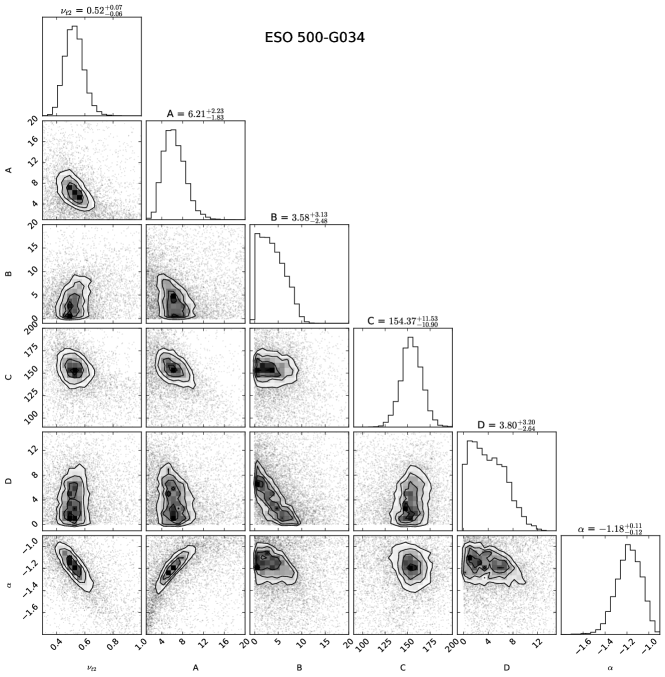
Figure 15: Corner plots showing the one and two-dimensional posterior probability distribution of the estimated parameters in the radio SED modeling for LIRG ESO 500-G034. The complete figure set (11 images) is available in the online journal.

The best-fit radio SEDs are presented in Figure 1 while Table 4 gives the corresponding model parameters, along with the 1$\sigma$ uncertainties corresponding to the 16th and 84th percentile of the posterior distribution of the parameter. Our radio-only modeling separates the thermal and nonthermal components from the total emission. Using the best-fit model, we estimated total thermal(nonthermal) emission by setting the normalization of the nonthermal(thermal) component(s) to zero. Table 5 gives the total, thermal, and nonthermal fluxes at 1.4 GHz, derived from the radio-only SED modeling, along with the 1$\sigma$ uncertainties corresponding to the 16th and 84th percentile of the posterior distribution of the parameter. To assess the degeneracy caused by the number of free parameters in the best-fit model, we give corner plots for all our galaxies in Appendix (Figure 15). The complete figure set (11 images) is available in the online journal. Figure 15. The corner plot gives the one- and two- dimensional projections of the posterior probability distribution of parameters. Most of our corner plots show poorly constrained thermal components, most likely due to weaker thermal emission in the frequency range covered by our data. In Table 5, we also provide the 1.4 GHz thermal fraction ($TF_{1.4}$). The thermal fraction ($TF$) at a given frequency is the ratio of thermal radio emission to total radio emission (synchrotron and free-free emission). NGC 3508 shows an excellent fit to the single power law (PL) shape. Three other galaxies, NGC 6000, IR 16164$-$0746, and ESO 453-G005, are fitted with a single-component model without a turnover (SFG NC). The galaxies ESO 440-IG058, NGC 5135, IC 4280, and ESO 593-IG008 are fitted with the single-component model with low-frequency turnover (C). For galaxies ESO 500$-$G034 is best-fitted with a multiple component model characterized with a single relativistic electron population in two different star-forming regions (one region with no turnover at low frequencies and the other characterized by a turnover (C2 1SAN). For galaxies ESO 507$-$G070 and IR 18293$-$3413, the best fit model turned out to be multiple components, one characterized by different relativistic electron populations in two different star-forming regions (one region with no turnover at low frequencies and the other characterized by a turnover (C2 1SAN2). None of our galaxies fits with models described by a single relativistic electron population in two different star-forming regions with different optical depths (C2 1SA) and a multiple component model representing two different electron populations in the two distinct star-forming galaxies with different optical depths (C2).

Table 3: List of input parameters for CIGALE modeling

Parameters		Values
delayed star formation history + additional burst (Ciesla et al., 2015)
e-folding time of the main stellar population model [Myr]	$\tau_{main}$	300-15000 by a bin of 300
e-folding time of the late starburst population model [Myr]	$\tau_{burst}$	50-1000 by a bin of 50
mass fraction of the late burst population	$f_{burst}$	0.05, 0.1, 0.3, 0.6, 0.9
Age of the main stellar population in the galaxy [Myr]	age	1000, 2000, 3000, 4500, 5000, 6500, 10000, 12000
Age of the late burst [Myr]	age${}_{burst}$	10.0, 40.0, 80.0, 110, 150, 170
stellar synthesis population (Bruzual & Charlot, 2003a)
Initial mass function	IMF	(Salpeter, 1955)
Metallicity	$Z$	0.02
Separation age		1 Myr
dust attenuation laws (Calzetti et al., 2000)
Colour excess of young stars	E(B-V)	0.1-2 by a bin of 0.2
Reduction factor${}^{(iii)}$	f${}_{att}$	0.3, 0.44, 0.6,0.7
dust grain model; THEMIS (Jones et al., 2017)
fraction of small hydrocarbon solids	q${}_{hac}$	0.02, 0.06, 0.1,0.17, 0.24
Minimum radiation field	U${}_{min}$	1, 5, 10, 15, 20, 30
power law index of the radiation	$\alpha$	2
fraction illuminated from $U_{\mathrm{min}}$ to $U_{\mathrm{max}}$	$\gamma$	0.02,0.06,0.1,0.15,0.2
active nucleus model; Skirtor (Stalevski et al., 2012, 2016)
optical depth at 9.7$~{}\mu$m	$\tau_{9.7}$	3.0, 7.0
torus density radial parameter	pl	1.0
torus density angular parameter	q	1.0
angle between the equatorial plan and edge of the torus [deg]	oa	40
ratio of outer to inner radius	R	20
fraction of total dust mass inside clumps [%]	Mcl	97
inclination (viewing angle) [deg]	i	30 (type 1), 70 (type 2)
AGN fraction		0.0-0.4 by a bin of 0.05
extinction law of polar dust		SMC
E(B-V) of polar dust		0.01-0.7 by a bin of 0.5
Temperature of the polar dust	K	100
Emissivity index of the polar dust		1.6
synchrotron emission
FIR/radio parameter${}^{*}$	$q_{IR}$	2.3 - 2.9 by a bin of 0.1
Power-law slope (Flux $\propto$ Frequency${}^{\alpha_{synch}}$)	$\alpha_{synch}$	$-$1.8 to $-$0.2 by a bin of 0.1

${}^{*}$ computed as $\log_{10}L_{IR(8-1000\mu\rm m)}$ -$\log_{10}L_{1.4\,GHz}$ where $L_{1.4\,GHz}$ is the radio luminosity at 1.4 GHz.

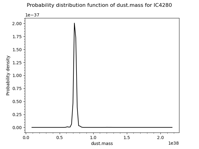
Figure 2: Probability distribution function (PDF) of the estimated dust mass for galaxy IC4280 using Bayesian inference.

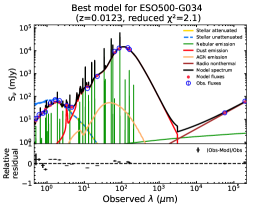
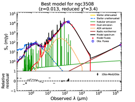
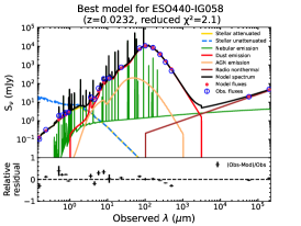
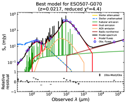
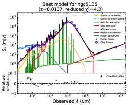
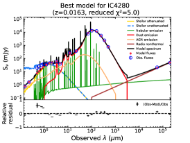
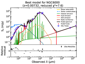
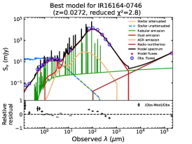
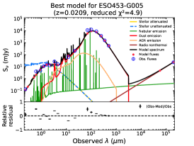
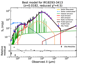
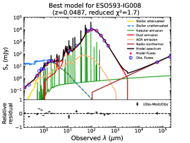
Figure 3: Best-fit CIGALE SEDs of the 11 LIRGs studied here. The open and filled symbols give the observed and modeled flux densities. The goodness of fit is estimated by reduced $\chi^{2}$ shown at the top of each panel, along with the name and redshift of the galaxy. In almost all cases, SEDs are well modeled, giving reasonable estimates of astrophysical properties.

4.2 UV to radio SED modeling with CIGALE

We estimate astrophysical properties of our galaxies using the SED fitting technique with the CIGALE version 2020.0 (Noll et al., 2009; Boquien et al., 2019). The CIGALE modeling works on the energy balance principle, i.e., the energy emitted by dust in the mid and far-$IR$ corresponds to the energy absorbed by dust in the $UV$ to optical range (Efstathiou & Rowan-Robinson, 2003). Moreover, it uses a Bayesian-like approach to model the SED and obtains the model parameters efficiently. CIGALE is parallelized and modular, which makes it user-friendly and efficient, as it does not solve the computationally demanding radiative transfer equation (Boquien et al., 2019). It provides the best fit model for the SED by selecting a suitable set of parameters. For this, a large grid of models is fitted to the data. The grid dimension is set by the number of input parameters used to define the different galaxy components, such as stellar emission spectra, star formation history, AGN emission, dust attenuation, nebular emission, and the slope of the radio synchrotron spectrum.

The interpretation of the observed SED is based on a comparison of all the modeled SEDs obtained from the fixed grid of parameters used for the modeling. First, each model is scaled and normalized to the data by minimizing $\chi^{2}$. Then the probability that a given model matches the data is quantified by the likelihood taken as e${}^{-\chi^{2}/2}$. These likelihoods can then be used as weights to estimate the physical parameters (the likelihood-weighted means of the physical parameters) and the related uncertainties (the likelihood-weighted standard deviation of the physical parameters). Finally, models with low probability are discarded, leaving only the best models to determine the physical parameters. Due to this process, the calculated uncertainties are symmetric (see also, Section 4.3 of Boquien et al., 2019). This method of choosing the best-fit model also takes care of the degeneracies in the model parameters, as only one parameter value (one with the highest probability in the pdf) can result in best-fit SED.

Next, we provide a brief account of the selected models used in our study.The first step towards obtaining the SED model requires building the stellar emission, which consists of selecting the single stellar population model (in our case; Bruzual & Charlot, 2003b), assuming Salpeter (1955) initial mass function. Next, to model the star formation history (SFH), we adopted a delayed SFR with an additional burst profile (in accordance to Małek et al., 2018). This form of SFH provides good estimates of the SFR-$M_{\star}$ relation compared to observations (Ciesla et al., 2015). The SFH is defined as:

$$\rm SFR\left(t\right)\propto\begin{cases}\rm SFR_{delayed}\left(t\right):\text{if}\,\,t<t_{0}.\\ \rm SFR_{delayed}\left(t\right)\,+\,\rm SFR_{burst}\left(t\right),:\text{if}\,\,t\geq t_{0}.\end{cases}$$ (11)

where $t_{0}$ is the age since the onset of the second episode (burst) of star formation.

To model starlight attenuation by dust, we chose the extinction law of Calzetti et al. (2000), and to model dust emission, we selected The Heterogeneous Evolution Model for Interstellar Solids (THEMIS; Jones et al., 2017) model. THEMIS successfully explains the observed Far-UV to Near-IR extinction and the shape of the IR to mm dust thermal emission. Furthermore, it predicts the observed relationship between the E(B-V) color excess and the inferred sub-mm opacity derived from Planck observation (see for information Jones et al., 2017; Nersesian et al., 2019). To incorporate the AGN component in the SED, we selected the SKIRTOR module (Stalevski et al., 2012, 2016). SKIRTOR is based on the 3D radiative transfer code SKIRT (Baes et al., 2011). It includes obscuration by dusty torus and obscuration by dust settled along with the polar directions. Since our galaxies have a rich amount of radio data, we used 1.4 GHz and 4.8 GHz fluxes to model the nonthermal synchrotron emission taking into account the power law of the synchrotron spectrum and the ratio of the far-IR/radio correlation in the CIGALE fitting.

Table 3 gives the set parameters used to build the SEDs of our galaxies. We adopted parameters similar to those used in Małek et al. (2017); Paspaliaris et al. (2021) and modified them accordingly to suit the galaxies in the current sample. The SED fitting was performed with a very careful adjustment of the fitting parameters, module by module. We performed the pdf analysis method to calculate the likelihood function ($\chi^{2}$) for all possible combinations of parameters (see Section 4.3 of Boquien et al., 2019). We generate the marginalized pdf for every parameter and assess the suitability of the SED model by visual inspection. An example of this method is given in Figure 2 for the galaxy IC4280 for dust mass. Figure 3 provides the CIGALE fit for our LIRGs. We note that some of the photometric data and the best model vary and, for them, the residuals exceed 20-30%. We want to stress that those residuals are often related to strong emission lines, visible for the nebular model. Moreover, this kind of catalog, which includes data from different surveys and instruments, sometimes performed more than 10–20 years ago (GALEX, XMM-OM), reduced with different reduction procedures, can result in heterogeneous photometric coverage of the spectra. In the SED fitting procedure, all measurements are treated with the same weight, and it can happen that the residuals of some of them are not as small as we would expect. The most significant residuals can be found for the $g^{\prime}$ and $r^{\prime}$ bands for our galaxies. As fits for the UV part of the spectra look very good, we can assume that the young stellar population was fitted with very good precision. The same observation can be made for $i^{\prime}$, $z^{\prime}$, and near-IR measurements, which assumes a good estimation of the stellar mass and properties of older stellar populations.

Another issue we want to address here is effect of different aperture sizes taken for flux measurements at different wavelengths for the SED modeling. Indeed, the apertures do not match for galaxies in our sample. The resulting SED fitting can be influenced by the decrement in the flux, especially nearby galaxies, where the beam size can be smaller than the galaxy itself. Also, a too large aperture in the case of a smaller galaxy can result in measuring a partial flux from another nearby galaxy. In our case, we tried to use an aperture size that was adequate to the size of a galaxy. Of course, it is impossible to match it perfectly without re-measuring fluxes, as was done in Ramos Padilla et al. (2020). As expected, this uncertainty in flux measurements results in errors for different estimated physical properties. In addition, CIGALE adds a 10% error to account for all these deviations. Problems with aperture, data reduction, and normalization can be seen as “jumps” in the SED instead of a smooth transition between different measurements. However, in the case of galaxies studied in this paper, the spectral coverage with broadband photometry is dense enough to obtain realistic physical properties. For the SED fitting procedure, fluxes were used together with the accompanying error. In our CIGALE analysis, we have also checked all pdfs for estimated physical properties such as stellar masses, star formation rate, dust mass, and dust temperature. We did not find any strange or suspicious behavior that incorrect photometric matching can trigger. We note that Ramos Padilla et al. (2020) showed, recalculating flux measurements can increase the quality of estimated astrophysical properties, however we did not remeasure the fluxes in our analysis.

Table 4: The most preferred models were selected on the basis of the Bayes odds ratio and the constrained value of the free parameters. The nominal value is taken as the 50${}^{th}$ percentile of the posterior distribution of the samples, and the 1$\sigma$ uncertainties are provided by the 16${}^{th}$ and 84${}^{th}$ percentile. Parameters not included in the models are indicated as “-”.

Name	Model	A	B	$\alpha$	$\nu_{t,1}$	C	D	$\alpha_{2}$	$\nu_{t,2}$
		(mJy)	(mJy)		(GHz)	(mJy)	(mJy)		(GHz)
(1)	(2)	(3)	(4)	(5)	(6)	(7)	(8)	(9)	(10)
ESO 500-G034	C2 1SAN	$6.21^{+2.23}_{-1.83}$	$3.58^{+3.13}_{-2.48}$	$-1.18^{+0.11}_{-0.12}$	-	$154.37^{+11.53}_{-10.90}$	$3.80^{+3.20}_{-2.64}$	-	$0.52^{+0.07}_{-0.06}$
NGC 3508	PL	$62.20^{+2.55}_{-2.31}$	-	$-0.73^{+0.02}_{-0.02}$	-	-	-	-	-
ESO 440-IG058	C	325.81${}^{+19.13}_{-16.75}$	$1.79^{+2.33}_{-1.28}$	$-0.82^{+0.03}_{-0.04}$	$0.14^{+0.02}_{-0.02}$	-	-	-	-
ESO 507-G070	C2 1SAN2	$39.95^{+4.46}_{-4.30}$	$5.10^{+3.25}_{-3.30}$	$-0.77^{+0.05}_{-0.06}$	-	$21.07^{+3.98}_{-4.20}$	$2.25^{+1.77}_{-1.53}$	$-1.50^{+0.38}_{-0.22}$	7.49${}^{+1.85}_{-2.01}$
NGC 5135	C	$1294.29^{+80.51}_{-70.09}$	$7.34^{+8.88}_{-5.28}$	$-0.88^{+0.03}_{-0.05}$	$0.13^{+0.02}_{-0.02}$	-	-	-	-
IC 4280	C	$359.44^{+43.22}_{-30.17}$	$10.43^{+5.69}_{-5.93}$	$-0.89^{+0.09}_{-0.12}$	$0.13^{+0.03}_{-0.03}$	-	-	-	-
NGC 6000	SFG NC	$144.60^{+3.21}_{-3.26}$	$0.48^{+0.34}_{-0.32}$	$-0.66^{+0.01}_{-0.02}$	-	-	-	-	-
IR 16164-0746	SFG NC	$61.52^{+2.27}_{-2.33}$	$0.49^{+0.36}_{0.33}$	$-0.45^{+0.03}_{-0.03}$	-	-	-	-	-
ESO 453-G005	SFG NC	$22.34^{+1.06}_{-0.99}$	$0.52^{+0.32}_{-0.35}$	$-0.59^{+0.04}_{-0.04}$	-	-	-	-	-
IR 18293-3413	C2 1SAN2	$34.13^{+12.20}_{-9.91}$	$4.09^{+3.28}_{-2.75}$	$-1.33^{+0.12}_{-0.14}$	-	$373.64^{+42.37}_{-41.82}$	$4.19^{+3.08}_{-2.79}$	$-1.74^{+0.08}_{-0.05}$	$1.06^{+0.08}_{-0.09}$
ESO 593-IG008	C	$540.79^{+73.47}_{-47.65}$	$0.49^{+0.34}_{-0.34}$	$-0.87^{+0.03}_{-0.03}$	$0.10^{+0.02}_{-0.02}$	-	-	-	-

Columns: (1) galaxy name, (2) best-fit model, (3) and (7) nonthermal normalization components, (4) and (8) thermal normalisation components, (5) and (9) synchrotron spectral indices, (6) and (10) turnover frequencies.

Table 5: Total, thermal, and nonthermal fluxes estimated at 1.4 GHz from the radio-only SED fitting and the corresponding thermal fraction estimated at 1.4 GHz. The nominal value is taken as the 50${}^{th}$ percentile of the posterior distribution of the samples, and the 1$\sigma$ uncertainties are provided by the 16${}^{th}$ and 84${}^{th}$ percentile.

Name	$S^{\rm total}_{1.4}$	$S^{th}_{1.4}$	$S^{\rm nth}_{1.4}$	$TF_{1.4}$
	(mJy)	(mJy)	(mJy)
(1)	(2)	(3)	(4)	(5)
ESO 500-G034	59.74${}^{+1.94}_{-1.74}$	7.32${}^{+1.82}_{-2.22}$	52.57${}^{+3.06}_{-2.74}$	0.11${}^{+0.02}_{-0.02}$
NGC 3508	61.84${}^{+2.55}_{-2.42}$	$-$	61.84${}^{+2.55}_{-2.42}$	0
ESO 440-IG058	49.98${}^{+1.03}_{-1.04}$	1.59${}^{+1.79}_{-1.13}$	48.39${}^{+1.66}_{-2.24}$	0.03${}^{+0.02}_{-0.02}$
ESO 507-G070	53.02${}^{+1.59}_{-1.59}$	4.75${}^{+3.41}_{-3.11}$	48.24${}^{+3.31}_{-3.52}$	0.09${}^{+0.04}_{-0.04}$
NGC 5135	164.33${}^{+3.58}_{-3.74}$	6.04${}^{+7.28}_{-4.43}$	158.29${}^{+6.20}_{-9.60}$	0.04${}^{+0.02}_{-0.03}$
IC 4280	50.32${}^{+1.52}_{-1.73}$	8.53${}^{+5.04}_{-5.17}$	41.84${}^{+6.12}_{-6.24}$	0.12${}^{+0.04}_{-0.04}$
NGC 6000	146.98${}^{+3.07}_{-3.21}$	0.49${}^{+0.35}_{-0.33}$	146.00${}^{+4.00}_{-3.00}$	0.003${}^{0.002}_{0.002}$
IR 16164-0746	62.04${}^{+2.45}_{-2.59}$	0.51${}^{+0.34}_{-0.33}$	61.50${}^{+2.50}_{-2.60}$	0.008${}^{+0.004}_{-0.004}$
ESO 453-G005	23.04${}^{+1.35}_{-1.24}$	0.52${}^{+0.33}_{-0.35}$	22.50${}_{+1.40}^{-1.40}$	0.02${}^{+0.01}_{-0.01}$
IR 18293-3413	220.59${}^{+7.18}_{-7.23}$	7.76${}^{+2.10}_{-2.15}$	212.84${}^{+7.95}_{-7.75}$	0.04${}^{+0.01}_{-0.01}$
ESO 593-IG008	58.59${}^{+1.72}_{-1.67}$	0.36${}^{+0.25}_{-0.26}$	58.22${}^{+1.70}_{-1.71}$	0.006${}^{+0.003}_{-0.003}$

Columns: (1) galaxy name, (2–4) total, thermal, and nonthermal fluxes at 1.4 GHz, (5) thermal fraction at 1.4 GHz

Table 6: CIGALE SED fit results.

Name	$\log_{10}(M_{\star})$	$\log_{10}(M_{\rm dust})$	$T_{\rm dust}$	$\log_{10}(\rm SFR_{\it IR})$	AGN fraction	$\alpha_{\rm synch}$	$\log_{10}(L_{\rm dust}$)	$q_{IR}$	$\chi^{2}$
	($M_{\odot}$)	($M_{\odot}$)	(K)	($M_{\odot}\,\rm yr^{-1}$)	(%)		($L_{\odot}$)
(1)	(2)	(3)	(4)	(5)	(6)	(7)	(8)	(9)
ESO 500-G034	10.12 $\pm$ 0.07	7.37 $\pm$ 0.04	27.55 $\pm$ 0.42	0.72 $\pm$ 0.14	1.11 $\pm$ 0.4	$-$0.90$\pm$0.04	11.86 $\pm$ 0.02	2.30 $\pm$ 0.01	2.1
NGC 3508	10.32 $\pm$ 0.02	7.68 $\pm$ 0.02	24.16 $\pm$ 0.02	0.59 $\pm$ 0.02	6.00 $\pm$ 0.001	$-$0.61 $\pm$0.03	11.25 $\pm$ 0.02	2.43 $\pm$ 0.04	3.4
ESO 440-IG058	9.51 $\pm$ 0.08	7.82 $\pm$ 0.02	27.24 $\pm$ 0.002	1.63 $\pm$ 0.02	4.53 $\pm$ 0.02	$-$1.20$\pm$0.09	10.99 $\pm$ 0.02	2.60 $\pm$ 0.05	2.1
ESO 507-G070	10.79 $\pm$ 0.02	7.61 $\pm$ 0.02	30.70 $\pm$ 0.003	1.35 $\pm$ 0.02	2.00 $\pm$ 0.0004	$-$0.74$\pm$0.08	10.93 $\pm$ 0.02	2.67 $\pm$ 0.05	4.4
NGC 5135	10.34 $\pm$ 0.03	7.89 $\pm$ 0.08	25.77 $\pm$ 1.52	1.05 $\pm$ 0.02	6.00 $\pm$ 0.04	$-$0.76$\pm$0.09	11.21 $\pm$ 0.02	2.50 $\pm$ 0.03	4.3
IC 4280	10.44 $\pm$ 0.06	7.66 $\pm$ 0.04	27.18 $\pm$ 0.50	1.07 $\pm$ 0.02	6.10 $\pm$ 0.60	$-$0.96$\pm$0.15	11.36 $\pm$ 0.02	2.30 $\pm$ 0.02	5.0
NGC 6000	10.32 $\pm$ 0.05	7.39 $\pm$ 0.05	28.91 $\pm$ 0.50	0.31 $\pm$ 0.12	1.06 $\pm$ 0.41	$-$0.90$\pm$0.03	10.79 $\pm$ 0.02	2.50 $\pm$ 0.02	7.6
IR 16164-0746	10.12 $\pm$ 0.06	7.82 $\pm$ 0.02	29.21 $\pm$ 0.003	1.52 $\pm$ 0.05	2.24 $\pm$ 0.01	$-$0.80$\pm$0.10	10.77 $\pm$ 0.02	2.45 $\pm$ 0.06	2.8
ESO 453-G005	9.62 $\pm$ 0.10	7.69 $\pm$ 0.02	27.24 $\pm$ 0.05	0.52 $\pm$ 0.20	4.72 $\pm$ 0.88	$-$0.82 $\pm$ 0.04	10.97 $\pm$ 0.02	2.50 $\pm$ 0.02	4.9
IR 18293-3413	10.67 $\pm$ 0.06	8.06 $\pm$ 0.02	30.70 $\pm$ 0.06	1.19 $\pm$ 0.32	2.55 $\pm$ 1.16	$-$1.19 $\pm$0.09	11.72 $\pm$ 0.02	2.60 $\pm$ 0.004	4.5
ESO 593-IG008	10.91 $\pm$ 0.19	8.30 $\pm$ 0.03	29.55 $\pm$ 0.40	1.71 $\pm$ 0.16	3.93 $\pm$ 2.7	$-$0.73 $\pm$0.68	11.18 $\pm$ 0.02	2.40 $\pm$ 0.001	1.7

Columns: (1) galaxy name, (2) stellar mass, (3) dust mass, (4) dust temperature, (5) instantaneous star formation rate, (6) AGN fraction, (7) slope of power-law synchrotron emission, $\alpha$, (8) dust luminosity, (9) $q_{IR}$, (10) reduced $\chi^{2}$ value for the best-fit model.

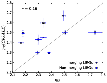
Figure 4: Comparison of $q_{IR}$ estimated by CIGALE modeling and Eq. 12. The grey line represents the one-to-one relation and the scatter, $\sigma$, from unity is given.

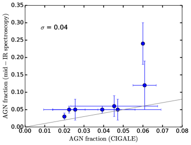
Figure 5: Comparison of bolometric AGN fractions obtained in this work and Díaz-Santos et al. (2017) for 8 LIRGs in our sample. The grey line represents the one-to-one relation and the scatter, $\sigma$, from unity is given.

Table 7: Emission Measure (EM) is derived from the model most supported by the evidence value for each source. Sources without constrained EM are marked by ‘–’

Name	EM${}_{1}$	EM${}_{2}$
	($10^{6}$ cm${}^{-6}$ pc)	($10^{6}$ cm${}^{-6}$ pc)
ESO 500-G034	$-$	0.77
NGC 3508	$-$	$-$
ESO 440-IG058	0.05	$-$
ESO 507-G070	$-$	269.5
NGC 5135	0.04	$-$
IC 4280	0.05	$-$
NGC 6000	$-$	$-$
IR 16164-0746	$-$	$-$
ESO 453-G005	$-$	$-$
IR 18293-3413	$-$	3.44
ESO 593-IG008	0.02	$-$

5 Results

5.1 Radio-only and FUV to radio SED modeling

The densely sampled radio-only and panchromatic (FUV to radio) SEDs for our sample are fitted with UltraNest and CIGALE modeling tools, respectively. Figures 1 and  3 present radio-only and FUV to radio spectral fits, respectively.  4 provides Bayesian estimates of the model parameters while and Table 6 provides frequentist estimates of the model parameters. Our main results are as follows:

1. The radio continuum SEDs of our galaxies covering $\sim$70 MHz-$\sim$15 GHz frequency range show a variety of features: (1) single PL model arising from synchrotron emission without thermal contribution, (2) single-component PL models due to synchrotron and free-free emission with and without turnover at low frequencies, and (3) two-component models with distinct emission regions, optical depths, and sometimes different spectral index of the CRe (Figure 1). The derived radio synchrotron spectral index ranges between $-$0.45${}_{-0.03}^{+0.03}$ and $-$1.74${}_{-0.08}^{+0.04}$. The turnover frequencies for SEDs fitted with models with absorption features fall in the range between 100${}_{-20}^{+20}$ MHz and 7.55${}_{-1.97}^{+1.94}$ GHz (Table 4).

2. Figure 3 provides the CIGALE fit for our LIRGs. CIGALE-modeling of the galaxies provides the rest-frame infrared luminosity in the wavelength range of 8-1000 $\mu$m (log${}_{10}L_{IR(8-1000\mu\,\rm m)}$) as 10.77$\pm$0.02 – 11.86$\pm$0.02 $L_{\odot}$. The $q_{IR}$ parameter is $\sim$2.30$\pm$0.02 – $\sim$2.67$\pm$0.05 while the radio spectral index estimated between 1.4 GHz and 5 GHz is in the range of $\sim-$0.61$\pm$0.03 – $-$1.20$\pm$0.09. The range of estimated stellar mass, dust mass, and dust temperature are $\log_{10}M_{\star}$ = 9.51$\pm$0.08 – 10.91$\pm$ 0.19 $M_{\odot}$, $\log_{10}M_{\rm dust}$ = 7.37$\pm$0.04 – 8.30$\pm$0.03  $M_{\odot}$, and $T_{\rm dust}$ = 24.16$\pm$0.02 – 30.70$\pm$0.06 K, respectively. The star formation rate $\log_{10}$SFR${}_{IR}$ is 0.31$\pm$0.12 – 1.71$\pm$0.16 ($M_{\odot}\,\rm yr^{-1}$). The AGN fraction that contributes to the optical and $IR$ emission ranges between 1.06$\pm$0.41% and 6.10$\pm$0.60% (Table 6).

3. Including the radio measurements in CIGALE modeling allowed us to obtain better constrained $L_{\rm dust}$ values as compared to CIGALE modeling results in the literature which did not include radio measurements. Although the dust luminosity of our galaxies falls in the range exhibited by galaxies of the same class, we note that our $L_{\rm dust}$ estimates have $\sim$1 order of magnitude lower uncertainties (0.02 dex, Table 6) than those provided in the literature ($\sim$0.2 dex from Małek et al., 2017).

4. Figure 4 shows the comparison between the $q_{IR}$ estimated from the CIGALE modeling and Eq. 12. The relation between these values is closer to unity and agree within errors, with a scatter (or average deviation), $\sigma$ = 0.16.

5. To cross-check the robustness of the CIGALE analysis, we present a comparison of the AGN fractions obtained for eight galaxies in our sample with the AGN fractions derived by Díaz-Santos et al. (2017) in Figure 5. CIGALE computes the AGN fraction using an AGN template that contributes between $UV$ and $IR$ wavelengths. In contrast, the Díaz-Santos et al. (2017) computes the AGN fraction using the mid-$IR$ (MIR) spectral diagnostics, including emission-line ratios, the equivalent width of 6.2 $\mu$m polycyclic aromatic hydrocarbon (PAH), the dust continuum slope at 30 and 15 $\mu$m as well as spectral template-based diagrams. The relation between the these values is closer to unity and they agree within error, with a scatter, $\sigma$=0.04. A close correspondence between our and Díaz-Santos et al. (2017) values validates the analysis procedure.

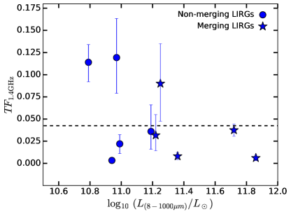
Figure 6: Thermal fraction ($TF$) at 1.4 GHz plotted against the rest-frame infrared luminosity obtained from our CIGALE modeling. The dashed line marks the average thermal fraction = 0.042 for our sample.

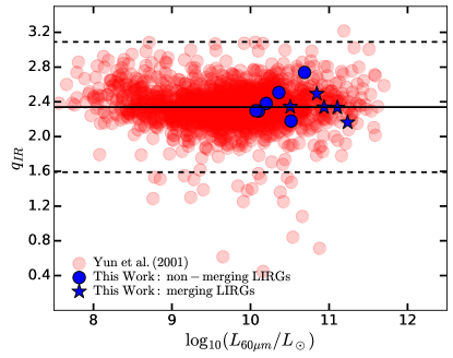
Figure 7: Distribution of $q_{IR}$ with 60 $\mu$m infrared luminosity for our sample of LIRGs. The solid horizontal line marks the mean $q_{IR}$ = 2.34 and the dashed lines represent upper and lower 3$\sigma$ bounds (Yun et al., 2001).

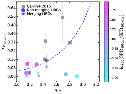
Figure 8: Distribution of thermal fraction with $q_{IR}$ (Eq. 12) for our sample of LIRGs. The color bar indicates the SFR${}_{IR}$ obtained for a time interval of 10 Myr ago from the CIGALE analysis. The dashed line marks the relation between thermal fraction and $q_{IR}$ given by $TF=$ $1.7\times$10${}^{q_{IR}-3.53}$ (Marvil et al., 2015).

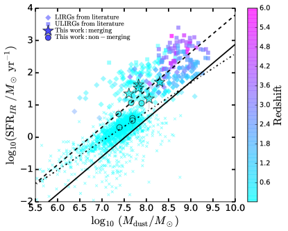
Figure 9: SFR${}_{IR}$ vs M${}_{\rm dust}$ for our sample of LIRGs obtained from CIGALE modeling. The solid and dashed lines, respectively, are the relations derived from low$-z$ dusty galaxies (H-ATLAS) and starburst galaxies (local ULIRGs and $z>$ 2 submillimeter galaxies) by Rowlands et al. (2014). The dot-dashed line represents the best-fit line to the SDSS-IRAS selected local star-forming galaxies of infrared luminosities (10$\leq$log${}_{10}$($L_{\rm dust}$/ $L_{\odot}$ $<$ 12) given by da Cunha et al. (2010)

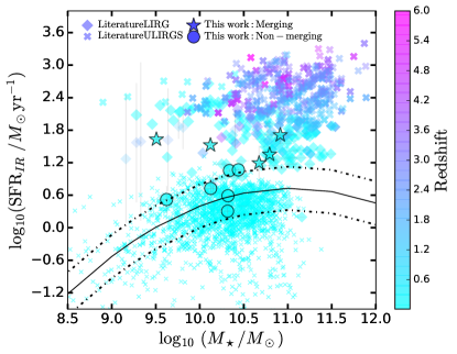
Figure 10: SFR${}_{IR}$ vs M${}_{\star}$ for our sample of LIRGs obtained from CIGALE modeling. The solid line represents the relation between M${}_{\star}$- SFR${}_{IR}$ for the main-sequence galaxies given by Schreiber et al. (2015) for a redshift range of 0.02. The dotted and dash-dotted lines show the range of the main sequence spreading $\pm$0.4 dex above and below the solid line.

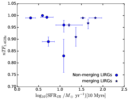
Figure 11: 1.4 GHz non-thermal fraction, $nTF$, as a function of SFR${}_{IR}$ for a time interval of 10 Myr. The nonthermal fraction is estimated in the same manner as that of the thermal fraction (see Section  6.2).

5.2 Specific results on individual galaxies

1. ESO 500-G034: classified as an intermediate between the Seyfert type AGN nucleus and a starburst galaxy (Hill et al., 1999), the densely sampled radio spectrum covering $\sim$2.3 decades in frequency (70 MHz-14.9 GHz) is fitted with a two-component model representing two distinct star-forming regions where the first component is without turnover. The turnover frequency is $\sim$0.52 GHz. The synchrotron spectral index, $\alpha$ = $-$1.15. The $TF$ at 1.4 GHz is $\sim$11.4%. The CIGALE modeling estimates a SFR${}_{IR}$ = 5.72 $M_{\odot}$ yr${}^{-1}$, high $L_{\rm dust}$ = 10${}^{11.86}$ $L_{\odot}$, and low AGN fraction = 1.11%, respectively. The low AGN fraction obtained by our analysis contradicts the previous results by Hill et al. (1999) who classified this source as an intermediate between an AGN and a starburst galaxy (its low is AGN fraction is also confirmed by Díaz-Santos et al., 2017).

2. NGC 3508: classified as a spiral galaxy (Veilleux et al., 1995), its densely sampled radio spectrum covering 2.9 decades in frequency (70 MHz-3 GHz) is fitted with a single component model characterized by synchrotron emission only. The synchrotron spectral index, $\alpha$ = $-$0.73. The $TF$ is 0 as this emission is characterized by synchrotron emission (i.e. no free-free component). The CIGALE modeling gives SFR${}_{IR}$ = 3.90 $M_{\odot}$ yr${}^{-1}$, $L_{\rm dust}$ = 10${}^{11.25}$ $L_{\odot}$, and AGN fraction = 6.00%, respectively, for this galaxy.

3. ESO 440-IG058: classified as a galaxy merger with a LINER-type AGN northern neighbor (Corbett et al., 2003), this galaxy is known to show shock-dominated emission for the southern system (Rodríguez-Zaurín et al., 2011). Its radio SED covering 2.1 decades (70 MHz-10.0 GHz) is fitted with single-component star-forming region properties (including absorption) with a turnover at $\sim$140 MHz. Synchrotron spectral index, $\alpha$ = $-$0.82. The computed $TF$ is 3.17%. The CIGALE-estimated SFR${}_{IR}$, $L_{\rm dust}$, AGN fraction are 42.66 $M_{\odot}$ yr${}^{-1}$, 10${}^{10.99}$ $L_{\odot}$, $\sim$4.53%, respectively. Our SFR${}_{IR}$ value is comparable within uncertainty to that obtained in literature ($\sim$36$\,M_{\odot}$ yr${}^{-1}$; Miluzio et al., 2013) and ($\sim$48$\,M_{\odot}$ yr${}^{-1}$; Herrero-Illana et al., 2017).

4. ESO 507-G070: classified as a Seyfert-type AGN nucleus (Condon et al., 1996) in a post-merger system (Stierwalt et al., 2013; Paspaliaris et al., 2021), its radio SED covering $\sim$2.3 decades in frequency (70 MHz-14.9 GHz) is best-fitted with a two-component model representing two distinct star-forming regions with different ultrarelativistic electron populations and high frequency turnover. The synchrotron spectral indices for the two populations, $\alpha$ and $\alpha_{2}$, are $-$0.77 and $-$1.50, respectively. The $TF$ is $\sim$9%. The SFR${}_{IR}$, $L_{\rm dust}$, AGN fraction are 22.40 $M_{\odot}$ yr${}^{-1}$, 10${}^{10.93}$ $L_{\odot}$, $\sim$2.0%, respectively. Its UV-$IR$ SED has previously been modeled with CIAGLE by Paspaliaris et al. (2021) who reported comparable $L_{\rm dust}$ (=10${}^{11.1}$ $L_{\odot}$), and SFR${}_{IR}$ (45.1 $M_{\odot}$ yr${}^{-1}$), and lower AGN fraction (0%) as compared to our results.

5. NGC 5135: classified as having a Seyfert-type AGN nucleus (Condon et al., 1996) with strong starburst along the spiral arms (Muñoz Marín et al., 2007), its radio SED covering $\sim$2.0 decades in frequency (70 MHz-6.7 GHz) is fitted with single-component star-forming region properties (including absorption) with a turnover at $\sim$0.130 GHz. The synchrotron spectral index, $\alpha$ = $-$0.88. The $TF$ is $\sim$3.6%. The CIGALE-estimated SFR${}_{IR}$, $L_{\rm dust}$, AGN fraction are 11.22 $M_{\odot}$ yr${}^{-1}$, 10 ${}^{11.21}$ $L_{\odot}$, $\sim$6%, respectively.

6. IC 4280: classified as a spiral galaxy (Fairall et al., 1989; Jin et al., 2019), its radio SED covering $\sim$1.6 decades (70 MHz-3.0 GHz) is best-fitted with a single-component star-forming region properties (including absorption) with a turnover at $\sim$140 MHz. The synchrotron spectral index, $\alpha$ = $-$0.9. The $TF$ is 11.9%. The CIGALE-estimated SFR, $L_{\rm dust}$, AGN fraction are 11.75 $M_{\odot}$ yr${}^{-1}$, 10${}^{11.36}$ $L_{\odot}$, $\sim$6%, respectively.

7. NGC 6000: classified as a starburst galaxy (Carollo et al., 2002), its radio SED covering $\sim$1.6 decades in frequency (70 MHz-3.0 GHz) is best-fitted with emission from a single star-forming region without a low frequency turnover. The synchrotron spectral index is $-$0.66. The $TF$ is 0.3%. The CIGALE-estimated SFR, $L_{\rm dust}$, and AGN fraction are 2.04 $M_{\odot}$ yr${}^{-1}$, 10 ${}^{10.79}$ $L_{\odot}$, $\sim$1.06%, respectively.

8. IR 16164-0746: classified as a late stage merger (Stierwalt et al., 2013) with a single LINER-type nucleus and a tidal-tail (Dixon & Joseph, 2011; Hung et al., 2015), its radio SED covering $\sim$1.6 decades in frequency (70 MHz-3.0 GHz) is best-fitted with emission from a single star-forming region without low frequency turnover. The synchrotron spectral index is $\sim$-0.5. The $TF$ is 0.8%. The CIGALE-estimated SFR, $L_{\rm dust}$, AGN fraction are 33.11 $M_{\odot}$ yr${}^{-1}$, 10 ${}^{10.77}$ $L_{\odot}$, $\sim$2.2%, respectively.

9. ESO 453-G005: a galaxy pair that appears to be dominated by star-forming activity, although it does not show signs of interaction (Rich et al., 2015), its poorly sampled radio SED covering $\sim$1.3 decades in frequency (150 MHz-3.0 GHz) is best-fitted with emission from a single star-forming region without a low-frequency turnover. The synchrotron spectral index is $\sim$-0.6. The $TF$ is 2%. The CIGALE-estimated SFR, $L_{\rm dust}$, AGN fraction are 3.31 $M_{\odot}$ yr${}^{-1}$, 10 ${}^{10.97}$ $L_{\odot}$, $\sim$4.7%, respectively.

10. IR 18293-3413: a complex system, classified both as early-merger (Haan et al., 2011) and mid-merger (Ricci et al., 2017) galaxy system with no evidence of AGN activity (X-ray spectrum; Risaliti et al., 2000), its radio SED covering $\sim$2.1 decades in frequency (70 MHz-8.4 GHz) is best-fitted with two-component model representing two distinct star-forming regions with different ultrarelativistic CRe and one region without any turnover. The synchrotron spectral indices for the two populations are, $-$1.33 and $-$1.74, respectively. The turnover frequency is 1.06 GHz. The $TF$ is $\sim$3.7%. The CIGALE-estimated SFR, $L_{\rm dust}$, AGN fraction are 15.48 $M_{\odot}$ yr${}^{-1}$, 10 ${}^{11.7}$ $L_{\odot}$, $\sim$2.5%, respectively.

11. ESO 593-IG008: known as the ‘Bird’ (Väisänen et al., 2017), this system is a a well-known galaxy merger (Stierwalt et al., 2013; Hung et al., 2015). Its radio SED covering 1.8 decades (70 MHz-4.8 GHz) is fitted with single-component star-forming region synchrotron (including absorption) with a turnover at $\sim$100 MHz. Synchrotron spectral index, $\alpha$ = $-$0.87. The computed $TF$ is 0.6%. The CIGALE-estimated SFR, $L_{\rm dust}$, AGN fraction are 51.3 $M_{\odot}$ yr${}^{-1}$, 10 ${}^{11.18}$ $L_{\odot}$, $\sim$3.9%, respectively.

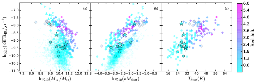
Figure 12: Distribution of sSFR${}_{IR}$ with respect to stellar mass (panel a), specific dust mass (panel b) and dust temperature (panel c) for the 11 LIRGs studied here (star and circle symbols represent the merging and non-merging types). For comparison, we include data from literature for normal star forming galaxies (cross; da Cunha et al., 2010), LIRGs (upward facing triangle; Vega et al., 2008), (circle; Paspaliaris et al., 2021), (diamond; da Cunha et al., 2015), (square; Lo Faro et al., 2013), and ULIRGs, (right side facing triangle; Vega et al., 2008), (plus; da Cunha et al., 2015).

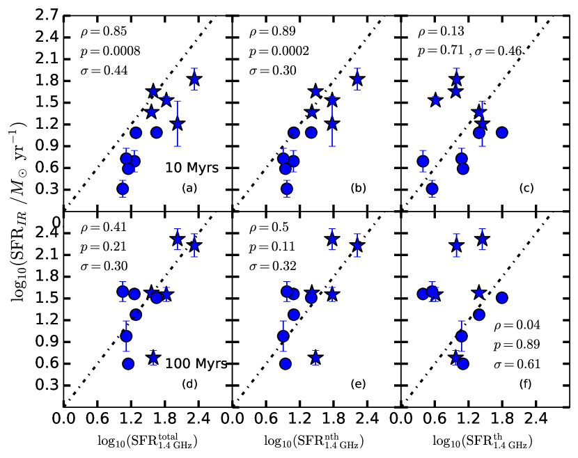
Figure 13: Comparison of the SFR${}_{IR}$ obtained for two time intervals 10 and 100 Myr ago from the CIGALE SED fitting and the 1.4 GHz radio SFR (total, nonthermal, and thermal, respectively). The mergers and non-mergers are shown with star and circle symbols, respectively. $p-$ and $\rho-$ values are obtained from the application of the Spearman’s rank correlation test while the scatter, $\sigma$, is the average deviation from the unity.

6 Discussion

6.1 $q_{IR}$ parameter

We estimate $q_{IR}$ using far-infrared fluxes at 60 $\mu$m and 100 $\mu$m and 1.4 GHz radio flux to compare with other samples in literature (Yun et al., 2001; Galvin et al., 2018). That is, we use the following expression given by Yun et al. (2001):

$$q_{IR}\equiv\log_{10}\left(\frac{\rm FIR}{3.75\times 10^{12}\,{\rm W\,m^{-2}}}\right)-\log_{10}\left(\frac{S_{\rm 1.4\,GHz}}{\rm W\,m^{-2}\,Hz^{-1}}\right)$$ (12)

The far infrared luminosity, FIR, is computed using ${\rm FIR}\equiv$1.26 $\times$10${}^{-14}$ (2.58 $S_{60\mu\rm m}$ + $S_{100\mu\rm m}$) W m${}^{-2}$ where $S_{60\mu\rm m}$ and $S_{100\mu\rm m}$ are the 60  and 100 $\mu\rm m$ band flux densities, in Jy, from IRAS. The error on q${}_{IR}$ parameter, computed using Eq. 12, is derived following standard error propagation. Figure 7 shows the distribution of log${}_{10}$ $q_{IR}$ obtained based on Eq. 12 with respect to monochromatic infrared luminosity at 60 $\mu\rm m$ ($=$4 $\pi$ $d_{L}^{2}$ $\times\,S_{60\mu\rm m}$ where $d_{L}$ is the luminosity distance). To obtain the luminosity distance, we use the cosmological calculator (Wright, 2006) with the Hubble constant $H_{0}=$ 69.6 km s${}^{-1}$ Mpc${}^{-1}$, $\Omega_{\rm M}=$ 0.286, and $\Omega_{\lambda}=$ 0.714 (Bennett et al., 2014). In this plot, the upper and lower dashed lines represent the 3$\sigma$ bounds of the mean value. The objects falling above and below the dashed lines are called the “IR excess” (upper dashed line) and the “radio excess” (lower dashed line), respectively. Our sample exhibits typical values of $q_{IR}$, indicating that radio emission is dominated by star-forming processes without any hint of abnormal behavior, such as AGN dominance or unusually high star-forming activity. This supports the results of our $UV$ to $IR$ fitting from CIGALE, where the median AGN fraction is $\sim$2.5%, and only for one source ESO 453-G005 it is close to $\sim$10%. Furthermore, the distribution of $q_{IR}$, with respect to log${}_{10}$ $L_{60\mu\rm m}/(L_{\odot})$ gives comparable results to those obtained for other LIRGs by Yun et al. (2001) and Galvin et al. (2018). According to the plot, the merging and non-merging galaxies take values from the main, most frequent range of $q_{IR}$ values and are indistinguishable in this aspect.

6.2 Thermal fraction

From the radio–SED modeling, we computed the thermal fraction at 1.4 GHz, $TF_{\rm 1.4GHz}$, for our sample which range between 0.003${}_{-0.002}^{+0.002}$ and 0.12${}_{-0.04}^{+0.04}$ (Table 5). We plot the $TF_{\rm 1.4GHz}$ against the rest frame infrared luminosity from CIGALE (Figure 6). Our values are similar to those obtained for a different sample of starburst galaxies, including LIRGs and ULIRGs (19 galaxies at median redshift equal to 0.09; Galvin et al., 2018). These values are also compatible with those obtained from normal star-forming galaxy samples (Niklas et al., 1997; Tabatabaei et al., 2017).

6.3 Radio spectral indices and spectral curvature

The integrated radio spectra for our sample of LIRGs show complex forms and are rarely described by single power-laws (Figure 1). Eight out of 11 galaxies show bends in their spectra which we model as arising due to free-free absorption. Here we mention that curvatures in radio SEDs can also occur if the refractive index of the medium is less than unity (Tsytovitch-Razin effect; Israel & Mahoney, 1990), and due to synchrotron self-absorption (SSA; Israel & Mahoney, 1990). For our galaxies, the radio surface brightness (=Peak flux/$\theta^{2}$, where flux is in Jy and $\theta$ is the size in arcsec of the source; for unresolved sources, we take the synthesized beam size as the upper limit for the size) is of the order of 10${}^{-2}$ (Table A1). For the SSA mechanism to be important at 100 MHz frequencies for our sources, unreasonably high magnetic field strengths $>$1000 G are needed (Kellermann & Pauliny-Toth, 1969). Therefore, SSA as a cause of turnover can be safely ruled out for our sample. The Razin turnover frequency is given as 20$\times\,n_{e}$/$B$(MHz), where $n_{e}$ is the electron density (cm${}^{-3}$) and $B$ is the magnetic field strength in $\mu$G (Ginzburg & Syrovatskii, 1965). In ISM, for the typical CRe density $\sim$1 (cm${}^{-3}$) (Ferrière, 2001) and the typical magnetic field strength of 50$\mu$G (Crocker et al., 2010), the Razin turnover frequency turns out to be 0.4 MHz. Therefore, we can safely rule out the Razin effect as a cause of low-frequency spectral turnover.

The synchrotron spectral index ranges between $\sim$$-$0.5 and $\sim$$-$1.7. The galaxies IR 16164$-$0746 and ESO 453-G005 have relatively flatter spectra, $\sim-$0.5, compared to the canonical value of $-$0.75 (Condon, 1992). For these galaxies, the spectral flattening can be ascribed to a change in the CRe spectrum (electron energy index =2.1) because of ionization losses (Lacki et al., 2010; Ramírez-Olivencia et al., 2022). Galaxies NGC 3508, ESO 440-IG058, NGC 5135, IC 4280, NGC 6000, and ESO 593-IG080 exhibit typical values of synchrotron spectral slope, ranging between $-$0.7 and $-$0.9. The remaining three galaxies, ESO 500-G034, ESO 507-G070, and IR 18293-3413, show steeper spectral slopes ranging between $-$1.17 and $-$1.74. Interestingly, galaxies showing stepper synchrotron spectral indices are fitted with two-component emission models. On the assumption that the injection indices of the electron energies are all similar but steepen due to physical processes, we expect the radiation spectral index to change by 0.5 due to synchrotron losses (Marvil et al., 2015). Therefore, within uncertainties, our spectral indices are consistent with a typical $\alpha$ $\sim$-0.75 and a value of $\alpha$ $\sim$ -1.25. The slightly flatter values are almost within the errors, which could be due to the complexity of the radio SED. We cannot evaluate it due to the poor spectral resolution achieved in our images. We speculate along the lines of Galvin et al. (2018) who also modeled the radio SED LIRGs that the CRe energy spectrum is intrinsically steep for these galaxies. We remark that, unlike frequent assumptions, the non-thermal spectral index is not fixed, and it changes between $-$0.45 and $-$1.75, which could be due to the influence of star formation on the energetics of CRe as discussed in Tabatabaei et al. (2017).

6.4 Emission measure

The emission measure (EM) is an integral of the electron density along the line of sight. EM is calculated by assuming that the emission originates from a cylindrical geometry with constant temperature and electron density (Condon, 1992). From the spectral turnover frequency, one can estimate the EM from the formula of the optical depth, $\tau_{\nu}$:

$$\tau_{\nu}=3.28\times\,10^{-7}\left(\frac{T_{e}}{10^{4}\,\rm K}\right)\,\left(\frac{\nu}{\rm GHz}\right)^{-2.1}\,\left(\frac{EM}{\rm pc\,cm^{-6}}\right)$$ (13)

where $T_{e}$ is the electron temperature of the H${}_{\textsc{II}}$ emitting region and $EM$ is the emission measure of depth $s$. $\tau_{\nu}$ is the optical depth, set at unity at turnover frequency measured from our SED modeling. The $EM$ is given by the integral of the electron density, $N_{e}$, along the line of sight of the $H_{\textsc{II}}$ region of depth $s$:

$$\frac{EM}{\rm pc\,cm^{-6}}=\int_{los}\,\left(\frac{N_{e}}{cm^{-3}}\right)^{2}\,d\left(\frac{s}{pc}\right)$$ (14)

We compute the EMs for our sources using the turnover frequencies obtained from our modeling (Table 4) and assuming a typical electron temperature 10${}^{4}$ K (Clemens et al., 2010; Galvin et al., 2018). Table 7 provides the emission measures for our sample. Our $EM$ values cover the same range as that obtained by Galvin et al. (19 LIRGs; 2018). Furthermore, our EM values are also consistent with those obtained by Clemens et al. (20 LIRGs and ULIRGs; 2010).

6.5 Thermal fraction vs. $q_{IR}$

In star forming galaxies the radio spectral index is expected to be correlated with $TF$ and $q_{IR}$ with the star formation history playing a key role (Marvil et al., 2015). This is because in young star forming galaxies ($<10^{8}$ yr; Condon (1992)) the radio emission is mainly due to free-free emission with a relatively flatter spectrum ($\alpha\sim-$0.1) leading to relatively higher values of $TF$ and $q_{IR}$ (Marvil et al., 2015). As the starburst ages, $TF$ and $q_{IR}$ are expected to decrease as the time-delayed nonthermal emission increases with time. This is mainly because the nonthermal emission originates from relatively old ($>10^{7}$ yr; the average lifespan of $>8\,M_{\odot}$OB type stars) relativistic electrons considering the time taken for the diffusion ($\sim\,10^{4}$ yr) of these electrons across the galaxy is negligible (Clemens et al., 2010; Galvin et al., 2018). Figure 8 shows the relation between $TF$ and $q_{IR}$ (computed using Eq. 12) as a function of the SFR${}_{IR}$ ratio obtained at time intervals 10 Myr and 100 Myr ago from the CIGALE analysis. This representation is informative in order to understand the evolution of the thermal fraction and $q_{IR}$ with the age of star formation. The large scatter observed in the plot can be explained by the following reasons: (i) ceasing of star formation before nonthermal emission commences, (ii) early contribution of nonthermal emission to the radio continuum while star formation is still ongoing, and (iii) due to limited sample size.

6.6 FR${}_{IR}$ vs. $M_{\rm dust}$

In Figure 9 we show the relation of SFR${}_{IR}$ with dust mass for our sample, including data from the literature for normal star-forming galaxies in the local Universe (da Cunha et al., 2010), LIRGs at low ($z<0.5$) and high ($z>0.5$) redshifts (Vega et al., 2008; Lo Faro et al., 2013; Pereira-Santaella et al., 2015; da Cunha et al., 2015; Małek et al., 2018; Paspaliaris et al., 2021), and ULIRGs at low and high redshifts (Vega et al., 2008; da Cunha et al., 2015; Małek et al., 2017, 2018). Our sample of LIRGs lies essentially in between the two sequences of normal and starburst galaxies defined by Rowlands et al. (2014), in excellent agreement with the behavior shown by starburst galaxies. This is because our $IR$ selection $S_{60\mu m}$ $\geq$5 Jy selects sources to have high SFRs. Moreover, our merger-type galaxies (filled star symbol) lie systematically higher in SFR${}_{IR}$ than the nonmergers (filled circle) and at the same time lie systematically below the high redshift LIRGs (diamonds) and ULIRGs (plus), while the normal star-forming galaxies (cross symbol) occupy the region characterized by a lower star formation rate and dust mass. This can be understood as follows. With an increase in the SFR${}_{IR}$, there is also an increase in the supernova rate, leading to a more efficient enrichment of the ISM with dust. Since SFR${}_{IR}$ is correlated with dust mass, and the dust relates the gas content in galaxies (Kennicutt relation links SFR${}_{IR}$ and gas mass), therefore, a positive trend in evolution of SFR${}_{IR}$ with dust mass is expected with our LIRGs when compared with local star-forming galaxies and ULIRGs (Rowlands et al., 2014; Donevski et al., 2020). High SFR${}_{IR}$ values are seen for interacting/merging LIRGs galaxies as compared to nonmergers (see also, Paspaliaris et al., 2021).

6.7 SFR${}_{IR}$ vs. stellar mass and nonthermal fraction

Figure 10 explores the relation of stellar mass with the CIGALE estimated star formation rate (SFR${}_{IR}$) for our galaxies, including the data for normal star-forming galaxies and the ULIRGs from the literature. As shown, our sample of LIRGs lies systematically above the main galaxy sequence represented by the parametric relation (solid line with 0.4 dex error denoted by dashed lines; Saintonge et al., 2016) along with local star-forming galaxies from the sample of da Cunha et al. (2010). There is no evidence of a correlation between stellar mass and SFR${}_{IR}$ for LIRGs and ULIRGs, including our sample (star symbol), which is explained by reaching saturation in SFR${}_{IR}$ and stellar mass for these types of galaxies (da Cunha et al., 2010; Paspaliaris et al., 2021). Figure 11 explores the relationship between the 1.4 GHz nonthermal fraction, $nTF$ (=nonthermal luminosity/total luminosity), and the SFR${}_{IR}$ for our galaxy sample. All galaxies, including merger and non-merger types in our sample, exhibit high $nTF$ values at 1.4 GHz, as expected. As we see a clear distinction between the SFR${}_{IR}$ values for merger- and non-merger-type galaxies, with the higher SFR${}_{IR}$ values being exhibited by merger-type galaxies, one would expect stronger magnetic fields $B$ in these objects due to strong turbulence created by the merger process. For a given synchrotron lifetime of CRe, $\tau_{synch}$ $\propto B^{-1.5}$, the CRe have a good chance to efficiently lose their energy via synchrotron radiation before escaping the star-forming regions.

In this regard, we note that resolved studies show that the radio spectral index is flatter in star-forming regions (Fletcher et al., 2011; Tabatabaei et al., 2007, 2013; Hassani et al., 2022) which contradicts the claimed argument of complete synchrotron cooling of CRes before escape from star-forming regions. Moreover, in star-forming regions, there is also a strong chance of CRe escape due to star formation feedback (Murphy et al., 2008). A fine balance between gas and magnetic fields/CRes can more realistically explain the nTF-SFR${}_{IR}$ correlation observed in normal star-forming galaxies (Tabatabaei et al. (2013) and Lacki et al. (2010)).

6.8 Specific star formation rate

Figure 12 shows the evolution of specific star formation rate, (sSFR${}_{IR}$ defined to be ratio of SFR${}_{IR}$ and $M_{\star}$), with respect $M_{\star}$ (panel a), specific dust mass ($sM_{\rm dust}$ defined to be ratio of $M_{\rm dust}$ and $M_{\star}$; panel b), and $T_{\rm dust}$ (panel c), respectively, for our sample of LIRGs including the data from the literature for normal star-forming galaxies along with LIRGs and ULIRGs. The sSFR${}_{IR}$ measures the recent star formation activity and is defined as the current star formation over the stellar mass of the galaxy (Donevski et al., 2020; Paspaliaris et al., 2021). Panel (a) shows an anticorrelation between the sSFR${}_{IR}$ and M${}_{\star}$ for the three samples, indicating that massive galaxies are less efficient in star formation than less-massive ones. This is expected in the ‘downsizing’ scenario of galaxy evolution, where massive galaxies formed most of their stars earlier and on shorter timescales. In comparison, less-massive galaxies evolve on longer timescales (Scodeggio et al., 2009; Popesso et al., 2011; Sobral et al., 2011; Laganá & Ulmer, 2018).

Panel (b) shows a positive correlation between sSFR${}_{IR}$ and $sM_{\rm dust}$ for the three samples, with LIRGs and ULIRGs occupying higher sSFR${}_{IR}$ values per unit of specific M${}_{\rm dust}$ compared to normal star-forming galaxies. In this plot, the contribution of M${}_{\star}$ to SFR${}_{IR}$ and M${}_{\rm dust}$ is normalized, making it ideal for studying gas-to-dust behavior in galaxies (Smith et al., 2012; Hunt et al., 2014; Donevski et al., 2020). First, the figure shows that there is an increase in dust mass compared to stellar mass on a very short timescale for these galaxies with LIRGs and ULIRGs expected to occupy the top-right corner of the plot (see, Donevski et al., 2020, and the references therein). The relationship between sMdust and sSFR${}_{IR}$ indicates an evolutionary scenario where sSFR${}_{IR}$ decreases due to exhaustion of the gas reservoir and therefore causes an inefficient dust production, causing galaxies to occupy the bottom left corner of the plot (Burgarella et al., 2020). As expected, our LIRGs follow the trend, and local and high redshift LIRGs and ULIRGs with normal star-forming galaxies are in a different branch.

Panel (c) shows the distribution of sSFR${}_{IR}$ with $T_{\rm dust}$ for our LIRGs and local and high redshift LIRGs and ULIRGs obtained from the literature. We note that the dust temperature obtained for our LIRGs falls in a narrow range. This is most likely due to the discrete nature of the parameter space used in the CIGALE modeling, including the values provided for the interstellar radiation field needed to heat the dust (Eq. 1 of; Paspaliaris et al., 2021). In general, a linear trend is observed between sSFR${}_{IR}$ with $T_{\rm dust}$, extending to high$z$ galaxies, which is due to the heating of dust surrounding the young stellar population in highly star-forming galaxies (Magnelli et al., 2014; Liang et al., 2019). However, our sample has more homogeneous properties and indicates dust temperature within a limited range of 24 K to 32 K.

This comparison indicates that our galaxies fall in the middle of the parameter space occupied by normal galaxies of the local Universe and distant starburst objects, exhibiting intermediate properties, as expected, between the two extremes of the galaxy evolution.

6.9 Calibrating SFR in radio wavelength

Our detailed radio SED modeling enabled us to decompose the nonthermal and thermal spectral luminosities and derive the respective SFRs. For this, we use the radio SFR calibration relations given by Murphy et al. (2011). Thermal SFR, ${\rm SFR_{\nu}^{T}}$ is derived using Kroupa initial mass function (IMF; Kroupa, 2001) assuming solar metalicity and continuous star formation:

$$\left(\frac{\rm SFR_{\nu}^{T}}{M_{\sun}~{}{\rm yr^{-1}}}\right)=4.6\times 10^{-28}\left(\frac{T_{\rm e}}{10^{4}~{}{\rm K}}\right)^{-0.45}\left(\frac{\nu}{\rm GHz}\right)^{0.1}$$

$$\times\left(\frac{L_{\nu}^{\rm T}}{\rm erg~{}s^{-1}~{}Hz^{-1}}\right)\,$$ (15)

where $L_{\nu}^{\rm T}$ is the thermal spectral luminosity and $T_{e}$=10${}^{4}$ K.

The nonthermal SFR, ${\rm SFR_{\nu}^{NT}}$, is derived using calibration between the supernova rate and the SFR using the output of Starburst99 model (Leitherer et al., 1999), and empirical relation between supernova rate and nonthermal spectral luminosity, $L_{\nu}^{\rm NT}$, of the Milky Way (Tammann, 1982; Condon & Yin, 1990):

$$\left(\frac{\rm SFR_{\nu}^{NT}}{M_{\sun}~{}{\rm yr^{-1}}}\right)=6.64\times 10^{-29}\left(\frac{\nu}{\rm GHz}\right)^{\alpha^{\rm NT}}\left(\frac{L_{\nu}^{\rm NT}}{\rm erg~{}s^{-1}~{}Hz^{-1}}\right)$$ (16)

where, $\alpha^{\rm NT}$=$\alpha$=$\alpha_{synch}$ is the synchrotron spectral index. For our calculations, we use the values obtained from the radio SED modeling (Table 4).

The total SFR at 1.4 GHz, $\rm SFR_{\rm 1.4GHz}$ is derived using the relation between the IR emission and current SFR resulting from the integration of the output of Starburst99 spectrum over the wavelength range of 912 $\AA$ – 3646 $\AA$, and the q${}_{IR}$ relation (see eq. 12). We use q${}_{IR}$=2.64 (Bell, 2003) to arrive at the total $\rm SFR_{\rm 1.4GHz}$ relation:

$$\left(\frac{\rm SFR_{\rm 1.4GHz}}{M_{\sun}~{}{\rm yr^{-1}}}\right)=6.35\times 10^{-29}\left(\frac{L_{\rm 1.4GHz}}{\rm erg~{}s^{-1}~{}Hz^{-1}}\right)$$ (17)

Figure 13 shows the comparison of the SFR${}_{IR}$ obtained from the CIGALE SED fitting for two time intervals, 10 and 100 Myr ago, and the 1.4 GHz radio SFR (total, nonthermal, and thermal, respectively). Upon visual inspection, we observe that SFR${}_{IR}$ shows a one-to-one correlation with 1.4 GHz radio SFR, albeit with a large scatter, $\sigma$, which measures average deviation from the unity. A striking result is that we obtain a much better correspondence of radio emission (total and synchrotron) with the young stellar population of about 10 Myr than with the older population. To check this, we applied Spearman’s rank correlation test, which measures the statistical dependence between the two variables (Spearman, 1904). A null hypothesis of no correlation is tested against the alternate hypothesis of non-zero correlation at a certain significance level (=0.01, adopted by us). Typically, the $p-$value $<$0.01 means that the null hypothesis of no-correlation is rejected at a confidence level $>$99%. For the star formation rate at 10 Myr ago, the obtained $p-$values are 0.0008 and 0.0002, respectively, rejecting the null hypothesis that the radio (total, nonthermal, and thermal) and $IR$ SFRs are not correlated. At the same time, the $\rho$-values are positive, indicating a positive correlation between the two variables (panels a and b of Figure 13). The null hypothesis of no correlation is not rejected for a significance level of 0.01 for thermal SFR and SFR${}_{IR}$ at 10 Myr ago (panel c of Figure 13) and radio and SFR${}_{IR}$ at 100 Myr ago (panel d, e, f of Figure 13). This is probably due to the relatively short lifetime of the CRe synchrotron at the 1.4 GHz frequency. At this frequency, in a magnetic field of about 50$\mu$G (Crocker et al., 2010), the synchrotron lifetime is $\approx$ 3.3$\times$10${}^{5}$ yr. Therefore, synchrotron emission may be an effective indicator of recent SFR in galaxies. The thermal component appears to be less useful because of visible significant scatter in the predicted SFR. Since thermal emission is much weaker than synchrotron emission at this frequency, this may explain its weaker usefulness than the nonthermal component. Our analysis strengthens that 1.4 GHz radio SFR measurements can be used as a diagnostic tool for high-$z$ galaxies (Murphy et al., 2011; Tabatabaei et al., 2017).

6.10 Comparison of radio spectral indices from radio-only and CIGALE SED modeling

We emphasize that both radio-only and FUV to radio modeling includes synchrotron emission in the models, however, the direct comparison between the synchrotron spectral index obtained from the two SED fitting techniques is inadequate. This is because the CIGALE modeling (FUV to radio) uses a very simple formulation to compute the radio flux at 1.4 GHz. This is done using the standard $q_{IR}$ relation at 1.4 GHz and the integrated $IR$ luminosity between 8-1000$\mu$m. The radio flux at other frequencies is then computed using a single PL model with an assumed value of the spectral index. However, it is observed that the radio-only SEDs show complex morphologies (flattening or turnovers at lower frequencies and steepening at higher frequencies for some cases). Furthermore, such a direct comparison would only reveal the known scatter in the $q_{IR}$ relation (Wang et al., 2019; Sinha et al., 2022). Furthermore, the limitations of this simple extrapolation in the CIGALE modeling are evident by the discontinuities in the radio wavebands (Figure 3).

7 Conclusion and Final remarks

In this study, we performed joint modeling of SEDs of 11 LIRGs, focusing in radio-only and FUV to radio bands where model parameters are estimated using state-of-the-art Bayesian (radio-only) and Bayesian-like (CIGALE modeling) inference techniques. The radio-only SED modeling allowed us to decompose nonthermal and thermal radio components while the CIGALE modeling allowed us to fit complex star formation history models, i.e., delayed star formation with an exponential burst (in our case), enabling us to estimate SFR${}_{IR}$ at different time intervals. Our main finding are the following:

1. The radio-only SED modeling shows that radio spectra have complex features, showing bends and turnovers. Unlike the frequent assumptions, this shows that the nonthermal spectral index is not fixed, and it changes between $-$0.45 and $-$1.75, which could be due to the influence of star formation on the energetics of CRe. The computed 1.4 GHz $TF$ falls between $\sim$0.8% and $\sim$0.12% for our galaxies, similar to that obtained for other LIRGs in the literature.

2. Although many studies have performed FUV-$IR$ SED modeling using CIGALE for star-forming galaxies, LIRGs, and ULIRGs (see Section 1), only a handful include radio measurements in the SED fitting (e.g., Vega et al., 2008; Shen et al., 2020; Hamed et al., 2021). The inclusion of radio measurements in the CIGALE modeling mostly serves to better constrain the derived dust luminosity. Our results indicate that, while the values of $L_{IR}$, fall in the range exhibited by galaxies of the same class, the uncertainties on them are improved by one order of magnitude compared to those given in the literature.

3. The $M_{\star}$, $T_{\rm dust}$, SFR${}_{IR}$, and AGN fraction derived using CIGALE modeling for our galaxies falls in the range exhibited by galaxies of the same class. The AGN is not energetically dominant in our sources, as the typical AGN fraction is $\leq$ 6%, similar to those found in other samples. The bolometric AGN fraction obtained by CIGALE is similar to that obtained from spectroscopic methods for most of our galaxies, indicating the robustness of the CIGALE analysis.

4. Comparison of the 1.4 GHz radio SFRs obtained using the total, and nonthermal radio emissions shows a close correspondence with the CIGALE-obtained SFR${}_{IR}$ at 10 Myr ago as compared to 100 Myr ago, strengthening the view that 1.4 GHz SFR estimates is a good indicator of recent star formation.

The comparison of astrophysical properties obtained by radio-only SED modeling and CIGALE modeling with other samples studied in the literature indicates that our sample belongs to a homogeneous population of LIRGs with respect to their astrophysical properties. Finally, we end with an obvious caveat that our findings are based on a relatively small sample comprising 11 LIRGs in total and five merger-type galaxies. Therefore, a larger sample with broadband SED coverage is needed to strengthen the tentative findings presented in this study.

Appendix A Summary of radio observations gathered for radio SED modeling and optical–radio overlays

Tables  A1 and  A2 provide the basic information on the GMRT and VLA continuum datasets analysed by us while the Table A3 provides the integrated flux densities used in radio-only SED modeling. Figure 14 provides the overlay of the radio contours of DSS images for our galaxies. At the same time, the corner plots for the check on degeneracy on the model parameters are given in Figure 15.

Table A1: Primary and phase calibrators used in our GMRT observations.

Name	Primary (325 MHz)	Phase (325 MHz)	Primary (610 MHz)	Phase (610 MHz)
ESO 500$-$G034	3C 286, 3C 468.1	1130$-$148	3C 147, 3C 286	1130$-$148
NGC 3508	3C 286,3C 468.1	1130$-$148	3C 147, 3C 286	1130$-$148
ESO 440$-$IG058	3C 286, 3C 468.1	1248$-$199	3C 147, 3C 286	1248$-$199
ESO 507$-$G070	3C 286, 3C 468.1	1248$-$199	3C 147, 3C 286	1248$-$199
NGC 5135	3C 286, 3C 468.1	1248$-$199	3C 147, 3C 286	1248$-$199
IC 4280	3C 286, 3C 468.1	1248$-$199	3C 147, 3C 286	1248$-$199
NGC 6000	3C 286, 3C 468.1	1626$-$298	3C 147, 3C 286	1626$-$298
IR 16164$-$0746	3C 286, 3C 468.1	1626$-$298	3C 147, 3C 286	1626$-$298
ESO 453$-$G005	3C 286, 3C 468.1	1626$-$298	3C 147, 3C 286	1626$-$298
IR 18293$-$3413	3C 286, 3C 468.1	1830$-$360	3C 147, 3C 286	1830$-$360
ESO 593$-$IG008	3C 286, 3C 468.1	1830$-$360	3C 147, 3C 286	1830$-$360

Table A2: Summary of new GMRT and the archival VLA datasets analysed by us.

ID	Date of obs.	Tel.	Arr.	Frequency	$BW$	IF	Int.	rms	Synth. Beam	$PA$	S/N	Area
					(MHz)		(min)	$(\frac{\rm mJy}{\rm beam}$)	(${}^{\prime\prime}\times^{\prime\prime}$)	(${}^{\circ}$)		(arcsec${}^{2}$)
ESO 500-G034
23_051	2013 Jun 11	GMRT		325 MHz	32	1	32	0.78	12.49$\times$7.72	33.92	142	518.9
23_051	2012 Oct 20	GMRT		610 MHz	32	1	32	0.18	6.04$\times$4.27	$-$21.00	394	330.4
AC345	1993 May 24	VLA	CnB	1.4 GHz	50	2	2.5	0.50	25.13$\times$14.66	$-$21.90	22	1686.8
AD229	1989 Feb 20	VLA	BnA	4.8 GHz	50	2	7.5	0.14	1.67$\times$0.91	$-$61.11	79	11.1
AV186	1991 Mar 26	VLA	D	14.9 GHz	50	2	10.5	0.47	9.49$\times$4.85	$-$10.96	19	113.5
NGC 3508
23_051	2013 Jun 11	GMRT		325 MHz	32	1	32	0.84	10.94$\times$7.89	38.16	41	1703.1
23_051	2012 Oct 20	GMRT		610 MHz	32	1	32	0.31	5.63$\times$4.32	$-$34.77	42	997.5
AC205	1988 Mar 23	VLA	C	1.4 GHz	50	3.9	2	0.90	24.98$\times$16.46	$-$9.73	26	1729.7
ESO 440-IG058
23_051	2013 Jun 11	GMRT		325 MHz	32	1	32	0.60	10.94$\times$7.89	38.16	41	705.9
23_051	2012 Oct 20	GMRT		610 MHz	32	1	32	0.17	7.79$\times$4.20	$-$32.17	275	421.4
AS412	1990 Oct 6	VLA	CnB	1.4 GHz	50	2	7.9	0.28	21.50$\times$11.44	$-$48.59	30	1147.1
AS412	1990 Oct 6	VLA	CnB	4.8 GHz	50	2	7.5	0.11	6.59$\times$4.09	$-$44.93	92	187.1
ESO 507-G070
23_051	2013 Jun 11	GMRT		325 MHz	32	1	32	1.4	10.73$\times$8.11	4.80	81	466.2
23_051	2012 Oct 20	GMRT		610 MHz	32	1	32	0.67	7.35$\times$4.11	$-$43.75	190	174.5
AR531	2003 Nov 1	VLA	B	1.4 GHz	50	2	10.5	0.45	8.18$\times$5.47	12.12	165	177.2
AD215	1988 Jun 9	VLA	DnC	4.8 GHz	50	2	9.3	0.15	13.69$\times$12.64	$-$60.82	190	794.9
AV186	1991 Mar 26	VLA	D	14.9 GHz	50	2	10	0.52	10.10$\times$4.67	$-$16.23	39	142.5
NGC 5135
23_051	2013 Jun 11	GMRT		325 MHz	32	1	32	1.8	11.96$\times$7.97	4.75	558	775.0
23_051	2012 Oct 20	GMRT		610 MHz	32	1	32	0.35	7.84$\times$4.13	$-$38.36	747	730.2
AW126	1985 Apr 1	VLA	BnA	1.4 GHz	50	2	14.6	0.23	5.22$\times$3.28	49.38	10	156.1
AC351	1993 Feb 4	VLA	BnA	4.8 GHz	50	2	18.3	0.1	1.53$\times$1.16	$-$63.68	316	34.4
IC 4280
23_051	2013 Jun 11	GMRT		325 MHz	32	1	32	0.59	11.95$\times$8.08	9.45	99	1226.3
23_051	2012 Oct 20	GMRT		610 MHz	32	1	32	0.23	7.21$\times$4.22	$-$39.93	99	995.6
AC345	1993 May 24	VLA	CnB	1.4 GHz	50	2	3.9	0.55	18.83$\times$14.30	$-$48.84	56	1114.6
AD215	1988 Jun 14	VLA	DnC	4.8 GHz	50	2	8.5	0.17	13.15$\times$10.61	$-$54.87	44	1251.0
NGC 6000
23_051	2012 Oct 20	GMRT		610 MHz	32	1	32	0.28	6.75$\times$4.36	$-$17.18	600	1333.1
AC345	1993 May 24	VLA	CnB	1.4 GHz	50	2	2	0.52	27.01$\times$12.43	$-$44.71	207	2970.5
AC326	1992 Jul 13	VLA	D	4.8 GHz	50	2	2	0.37	34.85$\times$16.08	18.22	156	2828.2
IR 16164$-$0746
23_051	2012 Oct 20	GMRT		610 MHz	32	1	32	1.3	5.54$\times$4.66	$-$17.18	152	127.8
AT149	1993 Apr 26	VLA	B	1.4 GHz	50	2	2.2	0.43	6.60$\times$5.54	$-$0.78	137	139.7
ESO 453-G005
23_051	2012 Oct 20	GMRT		610 MHz	32	1	32	0.35	8.10$\times$4.14	$-$32.73	100	227.4
AC345	1993 May 24	VLA	CnB	1.4 GHz	50	2	1.9	1.6	37.58$\times$11.48	$-$46.21	15	798.3
IR 18293$-$3413
23_051	2013 Jun 11	GMRT		325 MHz	32	1	32	1.7	14.20$\times$9.26	$-$5.84	423	836.7
23_051	2012 Oct 20	GMRT		610 MHz	32	1	32	1.2	13.34$\times$3.98	$-$47.24	200	687.9
AT0	1983 Nov 30	VLA	BnA	4.8 GHz	50	2	8.5	0.21	1.03$\times$0.43	8.44	23	11.1
AP534	2007 Jun 11	VLA	A	8.4 GHz	50	2	80.3	0.038	0.60$\times$0.24	6.59	53	10.1
ESO 593-IG008
23_051	2013 Jun 11	GMRT		325 MHz	32	1	32	0.62	11.15$\times$9.56	$-$19.53	226	667.8
23_051	2012 Oct 20	GMRT		610 MHz	32	1	32	0.34	10.19$\times$4.16	$-$53.63	134	404.3
AT149	1993 May 23	VLA	CnB	1.4 GHz	50	2	5.2	0.68	26.66$\times$12.93	33.36	75	1329.3
AF446	2007 Mar 29	VLA	D	4.8 GHz	50	2	3.6	1.1	31.22$\times$22.34	$-$25.85	226	1452.5

Note. — (1) proposal identifier of the observation, (2) date of observations, (3) telescope used, (4) configuration array used for VLA observations, (5) central frequency of observation, (6) bandwidth used, (7) number of sub bands used during the observation, (8) integration time used to image the target, (9) typical rms noise on image near to the target measured using TVSTAT, (10) synthesized beam achieved, (11) position angle of the restoring beam, measured counter-clockwise from the standard north direction, (12) signal to noise (S/N) ratio of the source detection (ratio of peak flux density of the source and the rms noise on the map), (12) integration area used in TVSTAT.

Table A3: Integrated radio flux densities used for the SED fitting.

Name	Obs. Freq.	S	error	Ref.
	(GHz)	(mJy)	(mJy)
ESO 500-G034	0.091	174.25	33.06	(a)
	0.122	153.25	21.27	(a)
	0.150	155.9	24.19	(b)
	0.158	144.25	17.01	(a)
	0.189	137.5	15.39	(a)
	0.219	122.5	13.48	(a)
	0.325	139.74	7.28	(c)
	0.610	108.21	5.46	(c)
	1.4	62.61	2.23	(d)
	3.0	26.184	2.67	(e)
	4.8	19.32	0.72	(d)
	14.9	9.67	0.88	(d)
NGC 3508	.074	560	70	(f)
	0.091	459.75	34.52	(a)
	0.122	339.75	17.53	(a)
	0.150	230.0	32.8	(b)
	0.158	288.25	10.30	(a)
	0.189	274.25	7.41	(a)
	0.219	245.25	7.13	(a)
	0.325	195.80	10.66	(c)
	0.610	135.92	7.15	(c)
	1.4	55.57	2.93	(d)
	3.0	3.13	0.41	(e)
ESO440-IG058	0.091	260.75	40.56	(a)
	0.122	205.5	28.18	(a)
	0.150	156	23.07	(b)
	0.158	195.5	21.70	(a)
	0.189	190.25	20.78	(a)
	0.219	172.75	18.21	(a)
	0.325	160.01	8.23	(c)
	0.610	97.36	4.92	(c)
	0.843	72.1	5.7	(g)
	1.4	49.795	1.64	(d)
	3.0	32.32	3.22	(e)
	4.8	19.71	0.68	(d)
	10.0	9.7	0.9	(h)
ESO 507-G070	0.091	389.25	54.62	(a)
	0.122	344	40.52	(a)
	0.150	160.0	23.56	(b)
	0.158	276.5	30.61	(a)
	0.189	238.75	29.15	(a)
	0.219	224.25	24.04	(a)
	0.325	117.14	6.90	(c)
	0.610	87.79	4.75	(c)
	1.4	55.12	1.93	(d)
	3.0	32.44	3.26	(e)
	4.8	36.3	1.15	(d)
	14.9	19.37	1.17	(d)
NGC 5135	0.091	1011.25	173.16	(a)
	0.122	890.25	91.63	(a)
	0.150	826.8	83.7	(b)
	0.158	777.50	78.90	(a)
	0.189	649.75	67.38	(a)
	0.219	663.25	66.80	(a)
	0.325	533.40	27.29	(c)
	0.610	370.32	18.61	(c)
	1.40	165.69	5.03	(d)
	2.31	100.00	17.20	(i)
	3.0	95.766	9.794	(e)
	4.80	58.51	1.82	(d)
	6.70	48.00	7.20	(j)
IC 4280	0.091	271.50	49.90	(a)
	0.122	283.75	35.56	(a)
	0.150	186.1	27.54	(b)
	0.158	222.75	25.13	(a)
	0.189	189.15	22.93	(a)
	0.219	162.00	17.45	(a)
	0.325	162.4	8.46	(c)
	0.610	109.63	5.68	(c)
	1.4	48.04	1.92	(d)
	3.0	28.183	4.87	(e)
NGC 6000	0.092	913	105.53	(a)
	0.122	727.75	77.61	(a)
	0.150	418.2	59.55	(b)
	0.158	586.25	61.00	(a)
	0.189	569.75	58.18	(a)
	0.220	494	50.05	(a)
	0.61	287.03	14.51	(c)
	1.4	153.32	7.86	(d)
	4.8	62.70	2.10	(d)
IR 16164-0746	0.091	191.25	58.92	(a)
	0.122	176.50	37.05	(a)
	0.150	151.5	21.88	(b)
	0.158	183.75	26.98	(a)
	0.189	154.75	22.18	(a)
	0.219	200.25	30.21	(a)
	0.61	88.17	5.49	(c)
	1.4	62.36	3.26	(d)
	3.0	44.12	4.45	(e)
ESO 453-G005	0.15	81.6	12.67	(b)
	0.61	38.21	2.17	(c)
	0.84	29.40	2.9	(g)
	1.40	23.39	2.55	(d)
	3.00	14.28	1.45	(e)
IR 18293-3413	0.091	1390	152.79	(a)
	0.122	1006.75	107.71	(a)
	0.150	780.4	111.26	(b)
	0.158	907	92.79	(a)
	0.189	832.25	84.61	(a)
	0.219	710.25	72.27	(a)
	0.325	458.96	23.45	(c)
	0.610	405.18	20.84	(c)
	1.4	226.8	10.56	(k)
	3	106.53	10.81	(e)
	4.8	36.58	2.18	(d)
	8.4	22.09	1.16	(d)
ESO 593-IG008	0.092	261.45	71.30	(a)
	0.122	379.5	53.73	(a)
	0.150	250.0	36.07	(b)
	0.158	289.5	34.07	(a)
	0.189	277.5	30.62	(a)
	0.220	240	25.86	(a)
	0.325	174.46	8.90	(c)
	0.61	116.29	5.93	(c)
	1.4	60.35	2.36	(d)
	3.0	20.867	2.23	(e)
	4.8	21.86	1.91	(d)

Note. — Columns: (1) source name; (2) observing frequency; (3) integrated flux density of the source (4) the error in the flux density including the absolute calibration uncertainty (Sect 3.1), (5) references - (a) GLEAM, (b)TGSS ADR1 (Intema et al., 2017), (c) current observations, (d)re-analysed VLA, (e) VLASS (Gordon et al., 2021), (f) VLSSr (Lane et al., 2014), (g) SUMSS (h) ATCA, (i) S-PASS (Meyers et al., 2017), (j) Effelsberg (Impellizzeri et al., 2008), (k) NVSS.

Fig. SetA2.1. ESO 500-G034

A2.2. NGC 3508

A2.3. ESO 440-IG058

A2.4. ESO 507-G070

A2.5. NGC 5135

A2.6. IC 4280

A2.7. NGC 6000

A2.8. IR 16164-0746

A2.9. ESO 453-G005

A2.10. IR 18293-3413

A2.11. ESO 593-IG008

Appendix B Summary of UV-IR observations gathered for SED modeling via CIGALE

Table A4 lists the basic information on the instruments used for gathering multiwavelength FUV–$IR$ datasets and Table LABEL:tab:UV-IRflux lists the flux densities used in CIGALE modeling.

Table A4: Basic information on the instruments/satellites used for UV-IR measurements in the CIGALE modeling

Instrument	Passbands	Central Wavelength	Resolution
		($\mu$m)	($\arcsec$)
(1)	(2)	(3)	(4)
GALEX${}^{a}$	FUV, NUV	0.15, 0.227	4.2, 5.3
XMM-OM${}^{b}$	UVW2, UVW1	0.212, 0.291	1.98, 2
Swift${}^{c}$	UVW2, UVM2, UVW1,	0.193, 0.225, 0.260,
Swift${}^{c}$	u, b, v	0.346, 0.439, 0.547	2.5 (at 350nm)${}^{\dagger}$
SMSS${}^{d}$	u, v, g, r, i, z	0.35, 0.38, 0.51, 0.62, 0.78, 0.92	3.1, 2.9, 2.6, 2.4, 2.3, 2.3
SDSS DR16${}^{e}$	$u^{\prime}$, $g^{\prime}$, $r^{\prime}$, $i^{\prime}$, $z^{\prime}$	0.354, 0.477, 0.623, 0.762, 0.913	1.53, 1.44, 1.32, 1.26, 1.29
2MASS${}^{f}$	J, H, Ks	1.235, 1.662, 2.15	2
WISE${}^{g}$	W1-W4	3.4, 4.6, 12, 22	6.1, 6.4, 6.5, 12
Spitzer-IRAC${}^{h}$	IRAC1 - IRAC4	3.56,4.52,5.73,7.91	1.66, 1.72, 1.88, 1.98
IRAS${}^{i}$	IRAS1 - IRAS4	12, 25, 60, 100	45, 45, 90, 180
AKARI${}^{j,k}$	N60, WIDE-S, WIDE-L, N160	65, 90, 140, 160	37,39,58,61
Herschel-PACS${}^{l}$	Blue, Green, Red	70, 100, 160	6, 7, 12
Herschel-SPIRE${}^{m,n}$	PSW, PMW, PLW	250, 350, 500	17.9, 24.2, 35.4

Columns: (1) name of the instrument/satellite (references for the instrument are given as superscript). ${}^{a}$Bianchi & GALEX Team (1999), ${}^{b}$Mason et al. (2001), ${}^{c}$(Poole et al., 2008), ${}^{d}$(Wolf et al., 2018), ${}^{e}$https://www.sdss.org/dr16/imaging/other_info/, ${}^{f}$ Jarrett et al. (2000), ${}^{g}$Wright et al. (2010), ${}^{h}$Fazio et al. (2004), ${}^{i}$Neugebauer et al. (1984), ${}^{j}$Murakami et al. (2007), ${}^{k}$Doi et al. (2015), ${}^{l}$Poglitsch et al. (2010), ${}^{m}$Griffin et al. (2010), ${}^{n}$ Smith et al. (2017), (2) name of the passband/filter used for observation, (3) central wavelength of the passband, (h) resolution (full width at half maximum). ${}^{\dagger}$https://swift.gsfc.nasa.gov/about_swift/uvot_desc.html

References

- Ahumada et al. (2020) Ahumada, R., Prieto, C. A., Almeida, A., et al. 2020, ApJS, 249, 3, doi: 10.3847/1538-4365/ab929e
- Baars et al. (1977) Baars, J. W. M., Genzel, R., Pauliny-Toth, I. I. K., & Witzel, A. 1977, A&A, 500, 135
- Baes et al. (2011) Baes, M., Verstappen, J., De Looze, I., et al. 2011, ApJS, 196, 22, doi: 10.1088/0067-0049/196/2/22
- Bell (2003) Bell, E. F. 2003, ApJ, 586, 794, doi: 10.1086/367829
- Bennett et al. (2014) Bennett, C. L., Larson, D., Weiland, J. L., & Hinshaw, G. 2014, ApJ, 794, 135, doi: 10.1088/0004-637X/794/2/135
- Bianchi & GALEX Team (1999) Bianchi, L., & GALEX Team. 1999, Mem. Soc. Astron. Italiana, 70, 365
- Boquien et al. (2019) Boquien, M., Burgarella, D., Roehlly, Y., et al. 2019, A&A, 622, A103, doi: 10.1051/0004-6361/201834156
- Briggs (1995) Briggs, D. S. 1995, in American Astronomical Society Meeting Abstracts, Vol. 187, American Astronomical Society Meeting Abstracts, 112.02
- Bruzual & Charlot (2003a) Bruzual, G., & Charlot, S. 2003a, MNRAS, 344, 1000, doi: 10.1046/j.1365-8711.2003.06897.x
- Bruzual & Charlot (2003b) —. 2003b, MNRAS, 344, 1000, doi: 10.1046/j.1365-8711.2003.06897.x
- Buchner (2021) Buchner, J. 2021, The Journal of Open Source Software, 6, 3001, doi: 10.21105/joss.03001
- Burgarella et al. (2020) Burgarella, D., Nanni, A., Hirashita, H., et al. 2020, A&A, 637, A32, doi: 10.1051/0004-6361/201937143
- Calzetti et al. (2000) Calzetti, D., Armus, L., Bohlin, R. C., et al. 2000, ApJ, 533, 682, doi: 10.1086/308692
- Carollo et al. (2002) Carollo, C. M., Stiavelli, M., Seigar, M., de Zeeuw, P. T., & Dejonghe, H. 2002, AJ, 123, 159, doi: 10.1086/324725
- Chu et al. (2017) Chu, J. K., Sanders, D. B., Larson, K. L., et al. 2017, ApJS, 229, 25, doi: 10.3847/1538-4365/aa5d15
- Chyży et al. (2018) Chyży, K. T., Jurusik, W., Piotrowska, J., et al. 2018, A&A, 619, A36, doi: 10.1051/0004-6361/201833133
- Ciesla et al. (2017) Ciesla, L., Elbaz, D., & Fensch, J. 2017, A&A, 608, A41, doi: 10.1051/0004-6361/201731036
- Ciesla et al. (2015) Ciesla, L., Charmandaris, V., Georgakakis, A., et al. 2015, A&A, 576, A10, doi: 10.1051/0004-6361/201425252
- Clemens et al. (2010) Clemens, M. S., Scaife, A., Vega, O., & Bressan, A. 2010, MNRAS, 405, 887, doi: 10.1111/j.1365-2966.2010.16534.x
- Clemens et al. (2008) Clemens, M. S., Vega, O., Bressan, A., et al. 2008, A&A, 477, 95, doi: 10.1051/0004-6361:20077224
- Cohen et al. (2007) Cohen, A. S., Lane, W. M., Cotton, W. D., et al. 2007, AJ, 134, 1245, doi: 10.1086/520719
- Condon (1992) Condon, J. J. 1992, ARA&A, 30, 575, doi: 10.1146/annurev.aa.30.090192.003043
- Condon et al. (1998) Condon, J. J., Cotton, W. D., Greisen, E. W., et al. 1998, AJ, 115, 1693, doi: 10.1086/300337
- Condon et al. (1990) Condon, J. J., Helou, G., Sanders, D. B., & Soifer, B. T. 1990, ApJS, 73, 359, doi: 10.1086/191472
- Condon et al. (1996) —. 1996, ApJS, 103, 81, doi: 10.1086/192270
- Condon & Yin (1990) Condon, J. J., & Yin, Q. F. 1990, ApJ, 357, 97, doi: 10.1086/168894
- Conroy (2013) Conroy, C. 2013, ARA&A, 51, 393, doi: 10.1146/annurev-astro-082812-141017
- Corbett et al. (2003) Corbett, E. A., Kewley, L., Appleton, P. N., et al. 2003, ApJ, 583, 670, doi: 10.1086/345414
- Crocker et al. (2010) Crocker, R. M., Jones, D. I., Melia, F., Ott, J., & Protheroe, R. J. 2010, Nature, 463, 65, doi: 10.1038/nature08635
- da Cunha et al. (2010) da Cunha, E., Eminian, C., Charlot, S., & Blaizot, J. 2010, MNRAS, 403, 1894, doi: 10.1111/j.1365-2966.2010.16344.x
- da Cunha et al. (2015) da Cunha, E., Walter, F., Smail, I. R., et al. 2015, ApJ, 806, 110, doi: 10.1088/0004-637X/806/1/110
- Díaz-Santos et al. (2017) Díaz-Santos, T., Armus, L., Charmandaris, V., et al. 2017, ApJ, 846, 32, doi: 10.3847/1538-4357/aa81d7
- Dixon & Joseph (2011) Dixon, T. G., & Joseph, R. D. 2011, ApJ, 740, 99, doi: 10.1088/0004-637X/740/2/99
- Doi et al. (2015) Doi, Y., Takita, S., Ootsubo, T., et al. 2015, PASJ, 67, 50, doi: 10.1093/pasj/psv022
- Donevski et al. (2020) Donevski, D., Lapi, A., Małek, K., et al. 2020, A&A, 644, A144, doi: 10.1051/0004-6361/202038405
- Efstathiou & Rowan-Robinson (2003) Efstathiou, A., & Rowan-Robinson, M. 2003, MNRAS, 343, 322, doi: 10.1046/j.1365-8711.2003.06679.x
- Fairall et al. (1989) Fairall, A. P., Vettolani, G., & Chincarini, G. 1989, A&AS, 78, 269
- Fazio et al. (2004) Fazio, G. G., Hora, J. L., Allen, L. E., et al. 2004, ApJS, 154, 10, doi: 10.1086/422843
- Ferrière (2001) Ferrière, K. M. 2001, Reviews of Modern Physics, 73, 1031, doi: 10.1103/RevModPhys.73.1031
- Fletcher et al. (2011) Fletcher, A., Beck, R., Shukurov, A., Berkhuijsen, E. M., & Horellou, C. 2011, MNRAS, 412, 2396, doi: 10.1111/j.1365-2966.2010.18065.x
- Galvin et al. (2018) Galvin, T. J., Seymour, N., Marvil, J., et al. 2018, MNRAS, 474, 779, doi: 10.1093/mnras/stx2613
- Ginzburg & Syrovatskii (1965) Ginzburg, V. L., & Syrovatskii, S. I. 1965, ARA&A, 3, 297, doi: 10.1146/annurev.aa.03.090165.001501
- Gordon et al. (2021) Gordon, Y. A., Boyce, M. M., O’Dea, C. P., et al. 2021, ApJS, 255, 30, doi: 10.3847/1538-4365/ac05c0
- Griffin et al. (2010) Griffin, M. J., Abergel, A., Abreu, A., et al. 2010, A&A, 518, L3, doi: 10.1051/0004-6361/201014519
- Haan et al. (2011) Haan, S., Surace, J. A., Armus, L., et al. 2011, AJ, 141, 100, doi: 10.1088/0004-6256/141/3/100
- Hamed et al. (2021) Hamed, M., Ciesla, L., Béthermin, M., et al. 2021, A&A, 646, A127, doi: 10.1051/0004-6361/202039577
- Hassani et al. (2022) Hassani, H., Tabatabaei, F., Hughes, A., et al. 2022, MNRAS, 510, 11, doi: 10.1093/mnras/stab3202
- Helou et al. (1988) Helou, G., Khan, I. R., Malek, L., & Boehmer, L. 1988, ApJS, 68, 151, doi: 10.1086/191285
- Helou et al. (1985) Helou, G., Soifer, B. T., & Rowan-Robinson, M. 1985, ApJ, 298, L7, doi: 10.1086/184556
- Herrero-Illana et al. (2017) Herrero-Illana, R., Pérez-Torres, M. Á., Randriamanakoto, Z., et al. 2017, MNRAS, 471, 1634, doi: 10.1093/mnras/stx1672
- Hill et al. (2001) Hill, T. L., Heisler, C. A., Norris, R. P., Reynolds, J. E., & Hunstead, R. W. 2001, AJ, 121, 128, doi: 10.1086/318051
- Hill et al. (1999) Hill, T. L., Heisler, C. A., Sutherland, R., & Hunstead, R. W. 1999, AJ, 117, 111, doi: 10.1086/300666
- Hung et al. (2015) Hung, C.-L., Rich, J. A., Yuan, T., et al. 2015, ApJ, 803, 62, doi: 10.1088/0004-637X/803/2/62
- Hunt et al. (2014) Hunt, L. K., Palazzi, E., Michałowski, M. J., et al. 2014, A&A, 565, A112, doi: 10.1051/0004-6361/201323340
- Hurley-Walker et al. (2017) Hurley-Walker, N., Callingham, J. R., Hancock, P. J., et al. 2017, MNRAS, 464, 1146, doi: 10.1093/mnras/stw2337
- Impellizzeri et al. (2008) Impellizzeri, C. M. V., Henkel, C., Roy, A. L., & Menten, K. M. 2008, A&A, 484, L43, doi: 10.1051/0004-6361:200809985
- Intema et al. (2017) Intema, H. T., Jagannathan, P., Mooley, K. P., & Frail, D. A. 2017, A&A, 598, A78, doi: 10.1051/0004-6361/201628536
- Israel & Mahoney (1990) Israel, F. P., & Mahoney, M. J. 1990, ApJ, 352, 30, doi: 10.1086/168513
- Jarrett et al. (2000) Jarrett, T. H., Chester, T., Cutri, R., et al. 2000, AJ, 119, 2498, doi: 10.1086/301330
- Jin et al. (2019) Jin, J.-J., Zhu, Y.-N., Wu, H., et al. 2019, ApJS, 244, 33, doi: 10.3847/1538-4365/ab3bfe
- Jones et al. (2017) Jones, A. P., Köhler, M., Ysard, N., Bocchio, M., & Verstraete, L. 2017, A&A, 602, A46, doi: 10.1051/0004-6361/201630225
- Kass & Raftery (1995) Kass, R. E., & Raftery, A. E. 1995, Journal of the American Statistical Association, 90, 773, doi: 10.1080/01621459.1995.10476572
- Kawada et al. (2007) Kawada, M., Baba, H., Barthel, P. D., et al. 2007, PASJ, 59, S389, doi: 10.1093/pasj/59.sp2.S389
- Kellermann & Pauliny-Toth (1969) Kellermann, K. I., & Pauliny-Toth, I. I. K. 1969, ApJ, 155, L71, doi: 10.1086/180305
- Kroupa (2001) Kroupa, P. 2001, MNRAS, 322, 231, doi: 10.1046/j.1365-8711.2001.04022.x
- Lacki et al. (2010) Lacki, B. C., Thompson, T. A., & Quataert, E. 2010, ApJ, 717, 1, doi: 10.1088/0004-637X/717/1/1
- Lacy et al. (2020) Lacy, M., Baum, S. A., Chandler, C. J., et al. 2020, PASP, 132, 035001, doi: 10.1088/1538-3873/ab63eb
- Laganá & Ulmer (2018) Laganá, T. F., & Ulmer, M. P. 2018, MNRAS, 475, 523, doi: 10.1093/mnras/stx3210
- Lane et al. (2014) Lane, W. M., Cotton, W. D., van Velzen, S., et al. 2014, MNRAS, 440, 327, doi: 10.1093/mnras/stu256
- Leitherer et al. (1999) Leitherer, C., Schaerer, D., Goldader, J. D., et al. 1999, ApJS, 123, 3, doi: 10.1086/313233
- Liang et al. (2019) Liang, L., Feldmann, R., Kereš, D., et al. 2019, MNRAS, 489, 1397, doi: 10.1093/mnras/stz2134
- Lo Faro et al. (2013) Lo Faro, B., Franceschini, A., Vaccari, M., et al. 2013, ApJ, 762, 108, doi: 10.1088/0004-637X/762/2/108
- Lonsdale et al. (2006) Lonsdale, C. J., Farrah, D., & Smith, H. E. 2006, Ultraluminous Infrared Galaxies, ed. J. W. Mason, 285, doi: 10.1007/3-540-30313-8_9
- Magnelli et al. (2014) Magnelli, B., Lutz, D., Saintonge, A., et al. 2014, A&A, 561, A86, doi: 10.1051/0004-6361/201322217
- Mainzer et al. (2011) Mainzer, A., Bauer, J., Grav, T., et al. 2011, ApJ, 731, 53, doi: 10.1088/0004-637X/731/1/53
- Małek et al. (2017) Małek, K., Bankowicz, M., Pollo, A., et al. 2017, A&A, 598, A1, doi: 10.1051/0004-6361/201527969
- Małek et al. (2018) Małek, K., Buat, V., Roehlly, Y., et al. 2018, A&A, 620, A50, doi: 10.1051/0004-6361/201833131
- Marvil et al. (2015) Marvil, J., Owen, F., & Eilek, J. 2015, AJ, 149, 32, doi: 10.1088/0004-6256/149/1/32
- Mason et al. (2001) Mason, K. O., Breeveld, A., Much, R., et al. 2001, A&A, 365, L36, doi: 10.1051/0004-6361:20000044
- Mauch et al. (2003) Mauch, T., Murphy, T., Buttery, H. J., et al. 2003, MNRAS, 342, 1117, doi: 10.1046/j.1365-8711.2003.06605.x
- Mauch et al. (2013) —. 2013, VizieR Online Data Catalog, VIII/81B
- Meyers et al. (2017) Meyers, B. W., Hurley-Walker, N., Hancock, P. J., et al. 2017, PASA, 34, e013, doi: 10.1017/pasa.2017.5
- Mhlahlo & Jamrozy (2021) Mhlahlo, N., & Jamrozy, M. 2021, MNRAS, 508, 2910, doi: 10.1093/mnras/stab2732
- Miluzio et al. (2013) Miluzio, M., Cappellaro, E., Botticella, M. T., et al. 2013, A&A, 554, A127, doi: 10.1051/0004-6361/201321192
- Muñoz Marín et al. (2007) Muñoz Marín, V. M., González Delgado, R. M., Schmitt, H. R., et al. 2007, AJ, 134, 648, doi: 10.1086/519448
- Murakami et al. (2007) Murakami, H., Baba, H., Barthel, P., et al. 2007, PASJ, 59, S369, doi: 10.1093/pasj/59.sp2.S369
- Murphy (2009) Murphy, E. J. 2009, ApJ, 706, 482, doi: 10.1088/0004-637X/706/1/482
- Murphy et al. (2008) Murphy, E. J., Helou, G., Kenney, J. D. P., Armus, L., & Braun, R. 2008, ApJ, 678, 828, doi: 10.1086/587123
- Murphy et al. (2011) Murphy, E. J., Condon, J. J., Schinnerer, E., et al. 2011, ApJ, 737, 67, doi: 10.1088/0004-637X/737/2/67
- NASA/IPAC Extragalactic Database (2019) (NED) NASA/IPAC Extragalactic Database (NED). 2019, NASA/IPAC Extragalactic Database (NED), IPAC, doi: 10.26132/NED1
- Nersesian et al. (2019) Nersesian, A., Xilouris, E. M., Bianchi, S., et al. 2019, A&A, 624, A80, doi: 10.1051/0004-6361/201935118
- Neugebauer et al. (1984) Neugebauer, G., Habing, H. J., van Duinen, R., et al. 1984, ApJ, 278, L1, doi: 10.1086/184209
- Niklas et al. (1997) Niklas, S., Klein, U., & Wielebinski, R. 1997, A&A, 322, 19
- Noll et al. (2009) Noll, S., Burgarella, D., Giovannoli, E., et al. 2009, A&A, 507, 1793, doi: 10.1051/0004-6361/200912497
- Ochsenbein (1996) Ochsenbein, F. 1996, The VizieR database of astronomical catalogues, CDS, Centre de Données astronomiques de Strasbourg, doi: 10.26093/CDS/VIZIER
- Page et al. (2012) Page, M. J., Brindle, C., Talavera, A., et al. 2012, MNRAS, 426, 903, doi: 10.1111/j.1365-2966.2012.21706.x
- Paspaliaris et al. (2021) Paspaliaris, E. D., Xilouris, E. M., Nersesian, A., et al. 2021, arXiv e-prints, arXiv:2102.03913. https://arxiv.org/abs/2102.03913
- Pearson et al. (2018) Pearson, W. J., Wang, L., Hurley, P. D., et al. 2018, A&A, 615, A146, doi: 10.1051/0004-6361/201832821
- Pereira-Santaella et al. (2011) Pereira-Santaella, M., Alonso-Herrero, A., Santos-Lleo, M., et al. 2011, A&A, 535, A93, doi: 10.1051/0004-6361/201117420
- Pereira-Santaella et al. (2015) Pereira-Santaella, M., Alonso-Herrero, A., Colina, L., et al. 2015, A&A, 577, A78, doi: 10.1051/0004-6361/201425359
- Pérez-Torres et al. (2021) Pérez-Torres, M., Mattila, S., Alonso-Herrero, A., Aalto, S., & Efstathiou, A. 2021, A&A Rev., 29, 2, doi: 10.1007/s00159-020-00128-x
- Perley & Butler (2017) Perley, R. A., & Butler, B. J. 2017, ApJS, 230, 7, doi: 10.3847/1538-4365/aa6df9
- Poglitsch et al. (2010) Poglitsch, A., Waelkens, C., Geis, N., et al. 2010, A&A, 518, L2, doi: 10.1051/0004-6361/201014535
- Poole et al. (2008) Poole, T. S., Breeveld, A. A., Page, M. J., et al. 2008, MNRAS, 383, 627, doi: 10.1111/j.1365-2966.2007.12563.x
- Popesso et al. (2011) Popesso, P., Rodighiero, G., Saintonge, A., et al. 2011, A&A, 532, A145, doi: 10.1051/0004-6361/201015672
- Ramírez-Olivencia et al. (2022) Ramírez-Olivencia, N., Varenius, E., Pérez-Torres, M., et al. 2022, A&A, 658, A4, doi: 10.1051/0004-6361/202140822
- Ramos Padilla et al. (2020) Ramos Padilla, A. F., Ashby, M. L. N., Smith, H. A., et al. 2020, MNRAS, 499, 4325, doi: 10.1093/mnras/staa2813
- Ricci et al. (2017) Ricci, C., Bauer, F. E., Treister, E., et al. 2017, MNRAS, 468, 1273, doi: 10.1093/mnras/stx173
- Riccio et al. (2021) Riccio, G., Małek, K., Nanni, A., et al. 2021, arXiv e-prints, arXiv:2106.12573. https://arxiv.org/abs/2106.12573
- Rich et al. (2015) Rich, J. A., Kewley, L. J., & Dopita, M. A. 2015, ApJS, 221, 28, doi: 10.1088/0067-0049/221/2/28
- Risaliti et al. (2000) Risaliti, G., Gilli, R., Maiolino, R., & Salvati, M. 2000, A&A, 357, 13. https://arxiv.org/abs/astro-ph/0002460
- Rodríguez-Zaurín et al. (2011) Rodríguez-Zaurín, J., Arribas, S., Monreal-Ibero, A., et al. 2011, A&A, 527, A60, doi: 10.1051/0004-6361/201014879
- Rowlands et al. (2014) Rowlands, K., Dunne, L., Dye, S., et al. 2014, MNRAS, 441, 1017, doi: 10.1093/mnras/stu510
- Saintonge et al. (2016) Saintonge, A., Catinella, B., Cortese, L., et al. 2016, MNRAS, 462, 1749, doi: 10.1093/mnras/stw1715
- Salpeter (1955) Salpeter, E. E. 1955, ApJ, 121, 161, doi: 10.1086/145971
- Sanders et al. (2003) Sanders, D. B., Mazzarella, J. M., Kim, D. C., Surace, J. A., & Soifer, B. T. 2003, AJ, 126, 1607, doi: 10.1086/376841
- Sanders & Mirabel (1996) Sanders, D. B., & Mirabel, I. F. 1996, ARA&A, 34, 749, doi: 10.1146/annurev.astro.34.1.749
- Schreiber et al. (2015) Schreiber, C., Pannella, M., Elbaz, D., et al. 2015, A&A, 575, A74, doi: 10.1051/0004-6361/201425017
- Scodeggio et al. (2009) Scodeggio, M., Vergani, D., Cucciati, O., et al. 2009, A&A, 501, 21, doi: 10.1051/0004-6361/200810511
- Serra et al. (2011) Serra, P., Amblard, A., Temi, P., et al. 2011, ApJ, 740, 22, doi: 10.1088/0004-637X/740/1/22
- Shen et al. (2020) Shen, L., Lemaux, B. C., Lubin, L. M., et al. 2020, MNRAS, 494, 5374, doi: 10.1093/mnras/staa1005
- Shirley et al. (2021) Shirley, R., Duncan, K., Campos Varillas, M. C., et al. 2021, arXiv e-prints, arXiv:2105.05659. https://arxiv.org/abs/2105.05659
- Sinha et al. (2022) Sinha, A., Basu, A., Datta, A., & Chakraborty, A. 2022, MNRAS, doi: 10.1093/mnras/stac1504
- Sirothia et al. (2014) Sirothia, S. K., Lecavelier des Etangs, A., Gopal-Krishna, Kantharia, N. G., & Ishwar-Chandra, C. H. 2014, A&A, 562, A108, doi: 10.1051/0004-6361/201321571
- Skilling (2004) Skilling, J. 2004, in American Institute of Physics Conference Series, Vol. 735, Bayesian Inference and Maximum Entropy Methods in Science and Engineering: 24th International Workshop on Bayesian Inference and Maximum Entropy Methods in Science and Engineering, ed. R. Fischer, R. Preuss, & U. V. Toussaint, 395–405, doi: 10.1063/1.1835238
- Skrutskie et al. (2006) Skrutskie, M. F., Cutri, R. M., Stiening, R., et al. 2006, AJ, 131, 1163, doi: 10.1086/498708
- Smith et al. (2012) Smith, D. J. B., Dunne, L., da Cunha, E., et al. 2012, MNRAS, 427, 703, doi: 10.1111/j.1365-2966.2012.21930.x
- Smith et al. (2017) Smith, M. W. L., Ibar, E., Maddox, S. J., et al. 2017, ApJS, 233, 26, doi: 10.3847/1538-4365/aa9b35
- Sobral et al. (2011) Sobral, D., Best, P. N., Smail, I., et al. 2011, MNRAS, 411, 675, doi: 10.1111/j.1365-2966.2010.17707.x
- Spearman (1904) Spearman, C. 1904, The American Journal of Psychology, 15, 72. http://www.jstor.org/stable/1412159
- Stalevski et al. (2012) Stalevski, M., Fritz, J., Baes, M., Nakos, T., & Popović, L. Č. 2012, MNRAS, 420, 2756, doi: 10.1111/j.1365-2966.2011.19775.x
- Stalevski et al. (2016) Stalevski, M., Ricci, C., Ueda, Y., et al. 2016, MNRAS, 458, 2288, doi: 10.1093/mnras/stw444
- Stierwalt et al. (2013) Stierwalt, S., Armus, L., Surace, J. A., et al. 2013, ApJS, 206, 1, doi: 10.1088/0067-0049/206/1/1
- Swarup (1990) Swarup, G. 1990, Indian Journal of Radio and Space Physics, 19, 493
- Tabatabaei et al. (2007) Tabatabaei, F. S., Beck, R., Krügel, E., et al. 2007, A&A, 475, 133, doi: 10.1051/0004-6361:20078174
- Tabatabaei et al. (2013) Tabatabaei, F. S., Schinnerer, E., Murphy, E. J., et al. 2013, A&A, 552, A19, doi: 10.1051/0004-6361/201220249
- Tabatabaei et al. (2017) Tabatabaei, F. S., Schinnerer, E., Krause, M., et al. 2017, ApJ, 836, 185, doi: 10.3847/1538-4357/836/2/185
- Tammann (1982) Tammann, G. A. 1982, in NATO Advanced Study Institute (ASI) Series C, Vol. 90, Supernovae: A Survey of Current Research, ed. M. J. Rees & R. J. Stoneham, 371–403
- Väisänen et al. (2017) Väisänen, P., Reunanen, J., Kotilainen, J., et al. 2017, MNRAS, 471, 2059, doi: 10.1093/mnras/stx1685
- Vardoulaki et al. (2015) Vardoulaki, E., Charmandaris, V., Murphy, E. J., et al. 2015, A&A, 574, A4, doi: 10.1051/0004-6361/201424125
- Vega et al. (2008) Vega, O., Clemens, M. S., Bressan, A., et al. 2008, A&A, 484, 631, doi: 10.1051/0004-6361:20078883
- Veilleux et al. (1995) Veilleux, S., Kim, D. C., Sanders, D. B., Mazzarella, J. M., & Soifer, B. T. 1995, ApJS, 98, 171, doi: 10.1086/192158
- Vika et al. (2017) Vika, M., Ciesla, L., Charmandaris, V., Xilouris, E. M., & Lebouteiller, V. 2017, A&A, 597, A51, doi: 10.1051/0004-6361/201629031
- Voelk (1989) Voelk, H. J. 1989, A&A, 218, 67
- Walcher et al. (2011) Walcher, J., Groves, B., Budavári, T., & Dale, D. 2011, Ap&SS, 331, 1, doi: 10.1007/s10509-010-0458-z
- Wang et al. (2019) Wang, L., Gao, F., Duncan, K. J., et al. 2019, A&A, 631, A109, doi: 10.1051/0004-6361/201935913
- Wayth et al. (2015) Wayth, R. B., Lenc, E., Bell, M. E., et al. 2015, PASA, 32, e025, doi: 10.1017/pasa.2015.26
- Wenger et al. (2000) Wenger, M., Ochsenbein, F., Egret, D., et al. 2000, A&AS, 143, 9, doi: 10.1051/aas:2000332
- Wolf et al. (2018) Wolf, C., Onken, C. A., Luvaul, L. C., et al. 2018, PASA, 35, e010, doi: 10.1017/pasa.2018.5
- Wright (2006) Wright, E. L. 2006, PASP, 118, 1711, doi: 10.1086/510102
- Wright et al. (2010) Wright, E. L., Eisenhardt, P. R. M., Mainzer, A. K., et al. 2010, AJ, 140, 1868, doi: 10.1088/0004-6256/140/6/1868
- Yershov (2014) Yershov, V. N. 2014, Ap&SS, 354, 97, doi: 10.1007/s10509-014-1944-5
- Yun et al. (2001) Yun, M. S., Reddy, N. A., & Condon, J. J. 2001, ApJ, 554, 803, doi: 10.1086/323145
- Żywucka et al. (2014) Żywucka, N., Goyal, A., Jamrozy, M., Ostrowski, M., & Stawarz, Ł. 2014, A&A, 563, A135, doi: 10.1051/0004-6361/201423500