A Time-Varying Cosmological Constant from Dynamical Chern-Simons Gravity

Abstract

We revisit the Kodama state by quantizing the theory of General Relativity (GR) with dynamical Chern-Simons (dCS) gravity. We find a new exact solution to the Wheeler-DeWitt equation where the Pontryagin term induces a modification in the Kodama state from quantizing GR alone. The dCS modification directly encodes the variation of the cosmological constant $\Lambda$.

I Introduction

While perturbative quantum gravity is non-renormalizable, one promising direction is to find a non-perturbative quantization of gravity that does not suffer from non-renormalizability. Approaches such as loop quantum gravity, causal dynamical triangulations, spin foam and causal sets are all non-perturbative approaches that attempt to yield a self-consistent quantization of gravity. Nonetheless, many of these approaches have had difficulties in making contact to a semi-classical limit.

Another promising non-perturbative quantization of General Relativity (GR) is to solve the Wheeler-DeWitt equation, which describes the quantum version of the Hamiltonian constraint, a linear combination of spatial and time diffeomorphism constraints that reflects the reparametrizability of GR under spatial and time coordinates. Solving the Wheeler-DeWitt equation amounts to finding the ground state of the theory. However, solving the Wheeler-DeWitt equation has proven to be insurmountable, with exception to minisuperspace approximations.

A major development was found by Kodama Kodama (1990) who used the Ashtekar formulation of classical GR to make the Wheeler-DeWitt equation tractible. Ashtekar re-expressed GR as a first-order Yang-Mills theory with a connection $A_{a}^{i}$ and its conjugate momentum $E_{a}^{i}$, which satisfy the canonical brackets $\{A_{a}^{i}(x),E_{k}^{b}(y)\}=8\pi G\delta_{a}^{b}\delta_{k}^{i}\delta^{3}(y,x)$ Ashtekar (1986). The Kodama state is an exact, non-perturbative solution with a positive cosmological constant.

While the Kodama state is a candidate for describing a ground state of quantum gravity with a positive cosmological constant non-perturbatively, it suffers from a number of issues, including non-normalizability, its CPT-violating properties (and consequent impossibility of having a positive energy), and lack of gauge invariance under large gauge transformations Magueijo (2021).

There are well-motivated reasons to consider modifications to GR, from anomaly cancellation to explaining observations such as leptogenesis and parity violation. In particular, dynamical Chern-Simons gravity (dCS) is a strong candidate to provide a modification to GR, a theory which has been studied and developed extensively Alexander and Yunes (2009). It has been theorized that chiral gravitational waves could emerge from dCS, where a change in a left-handed wave sources the right-handed wave and vice versa. Chiral gravitational waves could be a way to resolve the argument that the Kodama state is unphysical due to negative helicity states in the expansion of the Kodama state that result in negative energies; a state with negative energy could be recast as a positive-energy state with opposite helicity Witten (2003); Freidel and Smolin (2004).

In this note, we revisit the Kodama state by adding dCS into the gravitational theory and therefore into the Wheeler-DeWitt equation. We find a new exact solution to the Hamiltonian constraint such that the dCS modification allows for the time variation of the cosmological constant $\Lambda$.

II The New Hamiltonian Constraint and Wavefunction

We begin by considering the action Eq. (12) of Alexander et al. (2018), that of GR coupled to $N$ chiral fermion fields, all expressed in terms of Ashtekar variables (here $-\frac{3}{16\pi\Lambda G}\equiv\theta$) Samuel (1987); Jacobson and Smolin (1987):

$$S =\int_{M}\frac{1}{8\pi G}\bigg{\{}\epsilon^{abcd}e_{a}\wedge e_{b}\wedge e_{c}\wedge e_{d}\bigg{(}R+2\Lambda\bigg{)}$$

$$+\theta R^{AB}\wedge R_{AB}\bigg{\}}+\Sigma_{N}\overline{\Psi}_{A^{\prime}}\sigma_{a}^{A^{\prime}B}e^{a}\wedge(\mathcal{D}\Psi)_{B},$$ (1)

where we fix a topology $M=I\times\Sigma$, $I$ being the interval and we take $\Sigma$ to be compact. Notice the addition of the $\theta R^{AB}\wedge R_{AB}$ term in Eq. (1).
Applying a 3+1 decomposition to the action yields Alexander et al. (2018)

$$S =\int dt\bigg{[}\int_{\Sigma}\frac{1}{8\pi G}\bigg{(}E^{ai}\dot{A}_{ai}-\mathcal{N}\mathcal{H}-\mathcal{N}^{a}\mathcal{D}_{a}-\mu_{i}\mathcal{G}^{i}\bigg{)}$$

$$+\frac{3}{16\pi G}\frac{\dot{\Lambda}}{\Lambda^{2}}\int_{\Sigma}Y_{\text{CS}}(A)\bigg{]}.$$ (2)

So starting with the Hamiltonian from GR Smolin (2002),

$$\mathcal{H_{\text{GR}}}=\frac{1}{8\pi G}\epsilon_{ijk}E^{ai}E^{bj}\bigg{(}F_{ab}^{k}+\frac{\Lambda}{3}\epsilon_{abc}E^{ck}\bigg{)},$$ (3)

we add to it a Pontryagin term $\theta R^{AB}\wedge R_{AB}$. For this we can simply read off of Eq. (1); from Alexander et al. (2018), we see that the Pontryagin term contributes an additional term $\frac{3}{16\pi G}\frac{\dot{\Lambda}}{\Lambda^{2}}Y_{CS}(A)$ to the GR Hamiltonian, where $Y_{\text{CS}}(A)=\epsilon^{abc}F_{bc}^{i}A_{ai}$ is the Chern-Simons invariant of the Ashtekar connection. Using the fact that $\theta=-\frac{3}{16\Lambda\pi G}$, we have

$$\frac{\dot{\Lambda}}{\Lambda^{2}} =\frac{16\pi G}{3}\dot{\theta}.$$ (4)

Thus, the extra term in the Hamiltonian is

$$\mathcal{H}_{\text{DCS}}=\frac{3}{16\pi G}\frac{\dot{\Lambda}}{\Lambda^{2}}Y_{CS}(A)=\dot{\theta}Y_{CS}(A).$$ (5)

We apply the quantization procedure

$$\hat{E}^{ai}\rightarrow-G\frac{\delta}{\delta A_{ai}},$$ (6)

and the Hamiltonian constraint becomes

$$(\mathcal{H}_{\text{GR}}+\mathcal{H}_{\text{DCS}})\Psi(A)=0$$ (7)

$$\Rightarrow~{}- \dot{\theta}Y_{\text{CS}}(A)\Psi(A)=$$

$$\frac{G}{8\pi}\epsilon_{ijk}\frac{\delta}{\delta A_{ai}}\frac{\delta}{\delta A_{bj}}\bigg{(}F_{ab}^{k}-\frac{G\Lambda}{3}\epsilon_{abc}\frac{\delta}{\delta A_{ck}}\bigg{)}\Psi(A).$$ (8)

For $\Psi(A)$ we try the ansatz

$$\Psi(A)=\psi_{K}(A)\chi(A,\dot{\theta}),$$ (9)

where $\psi_{K}(A)\propto\text{exp}\bigg{(}\frac{3}{2G\Lambda}\int_{\Sigma}Y_{\text{CS}}(A)\bigg{)}$ is the solution to the Wheeler-DeWitt equation when the left-hand side of Eq. (8) is zero (i.e. without the inclusion of the Pontryagin term).
Plugging in our ansatz Eq. (9) into Eq. (8), we have

$$-\dot{\theta}Y_{\text{CS}}\psi_{K}\chi$$

$$=\epsilon_{ijk}\frac{G}{8\pi}\frac{\delta}{\delta A_{ai}}\frac{\delta}{\delta A_{bj}}\bigg{(}F_{ab}^{k}-\frac{G\Lambda}{3}\epsilon_{abc}\frac{\delta}{\delta A_{ck}}\bigg{)}\psi_{K}\chi.$$ (10)

We make the assumption that we are working with non-degenerate metrics, that is, $E\cdot E\sim\text{det}~{}g$. We also note that the terms in parentheses on the right-hand side of Eq. (10) annihilate $\psi_{K}$ by definition, and moreover we know that $G=M_{P}^{-2}$, where $M_{P}$ is the Planck mass. This means that Eq. (10) reduces to

$$\frac{\Lambda}{24\pi M_{P}}\chi^{\prime}+\bigg{(}\dot{\theta}Y_{CS}(A)+\frac{\epsilon_{ijk}M_{P}E^{ai}E^{bj}F_{ab}^{k}}{8\pi}\bigg{)}\chi=0,$$ (11)

where the primes denote derivatives with respect to $A$.
Here we also make the assumption that $F_{ab}^{k}$ is independent of $A$. This means we can set $F_{ab}^{k}$ equal to a constant; setting this constant equal to zero for simplicity, rearranging Eq. (11) and using the standard technique of separation of variables (again assuming that $E\cdot E\sim\text{det}~{}g$), we find

$$\chi(A,\dot{\theta})=\text{exp}\bigg{(}-\frac{24\pi M_{P}\dot{\theta}}{\Lambda}\int_{\Sigma}Y_{\text{CS}}(A)\bigg{)}.$$ (12)

Thus, the full wavefunction is

$$\Psi(A) =\psi_{K}(A)\chi(A,\dot{\theta})$$ (13)

$$=\text{exp}\bigg{[}\frac{3M_{P}^{2}}{2\Lambda}\bigg{(}1-\frac{16\pi\dot{\theta}}{M_{P}}\bigg{)}\int_{\Sigma}Y_{\text{CS}}(A)\bigg{]},$$ (14)

or in terms of $\dot{\Lambda}$,

$$\Psi(A)=\text{exp}\bigg{[}\frac{3M_{P}^{2}}{2\Lambda}\bigg{(}1-\frac{3\dot{\Lambda}}{\Lambda^{2}}M_{P}\bigg{)}\int_{\Sigma}Y_{CS}(A)\bigg{]}.$$ (15)

Eq. (12) is the modification to the Kodama state with the inclusion of the Pontryagin term (via Eq. (9)).

III Gauss and Diffeomorphism Constraints

We now want to see if the Gauss and spatial diffeomorphism constraints hold when the Kodama state gets modified with the Pontryagin term. From Eq. (2.5) of Soo (2002), the Gauss constraint is

$$D_{i}^{A}E^{ia}=0,$$ (16)

and the diffeomorphism constraint is

$$\epsilon_{ijk}E^{j}_{a}B^{ia}=0,$$ (17)

where {$E^{ia}(\textbf{x}),A_{jb}(\textbf{y})\}=i(8\pi G)\delta^{i}_{j}\delta^{a}_{b}\delta^{3}(\textbf{x}-\textbf{y})$.
We can define an operator $\hat{Q}^{ia}$ where

$$\hat{Q}^{ia}\equiv B^{ia}+\frac{\lambda}{3}\hat{E}^{ia}.$$ (18)

Plugging Eq. (18) into Eq. (16) yields, when acting on $\Psi(A)$,

$$D_{i}^{A}\hat{Q}^{ia}\Psi(A)=\frac{1}{2}D_{i}^{A}\epsilon^{ijk}F_{jk}^{a}\Psi(A),$$ (19)

where we used the fact that $B^{ia}=\frac{1}{2}\epsilon^{ijk}F_{jk}^{a}$. Since $D_{i}^{A}\epsilon^{ijk}F_{jk}^{a}=0$, we have that

$$D_{i}^{A}\hat{Q}^{ia}\Psi(A)=0.$$ (20)

As for the diffeomorphism constraint, we use Eq. (18) again, this time in Eq. (17), to find

$$\epsilon_{ijk}\hat{E}_{a}^{j}\hat{Q}^{ia}\Psi(A) =\frac{\lambda}{3}\epsilon_{ijk}\text{Tr}(\hat{E}^{j}\hat{E}^{i})\Psi(A)$$ (21)

which vanishes due to the symmetry of the frame fields. Therefore, we have

$$\epsilon_{ijk}\hat{E}_{a}^{j}\hat{Q}^{ia}\Psi(A)=0.$$ (22)

Eqs. (20) and (22) are exactly Eqs. (4.3) of Soo (2002). The Kodama state $\psi_{K}(A)$ satisfies Eqs. (20) and (22), by definition. However, since these constraints are trivially satisfied, this means that the modified Kodama state Eq. (14) would solve these constraints without modifying them. This also means that any $\Psi$ (and thus any modification to the Kodama state from GR) would satisfy the Gauss and diffeomorphism constraints unmodified, but $\Psi$ would have to solve the new modified Hamiltonian constraint (Eq. (8) in this case).

IV The Full Solution

Now we consider solving Eq. (11) without making the assumption that $F$ is independent of $A$. We have

$$\frac{1}{\chi}\chi^{\prime}=-\frac{24\pi M_{P}}{\Lambda}\bigg{(}\dot{\theta}Y_{CS}(A)+\frac{\epsilon_{ijk}M_{P}E^{ai}E^{bj}F_{ab}^{k}}{8\pi}\bigg{)},$$ (23)

so

$$\chi(A,\dot{\theta})=\text{exp}\bigg{[} -\frac{24\pi M_{P}\dot{\theta}}{\Lambda}\int_{\Sigma}Y_{CS}(A)$$

$$-\frac{3M_{P}^{2}}{\Lambda}\int_{\Sigma}\epsilon_{ijk}E^{ai}E^{bj}F_{ab}^{k}\bigg{]},$$ (24)

and the full Kodama state is

$$\Psi(A) =\psi_{K}(A)\chi(A,\dot{\theta})$$ (25)

$$=\text{exp}\bigg{\{}\frac{3M_{P}^{2}}{\Lambda}\bigg{[}\frac{1}{2}\bigg{(}1-\frac{16\pi\dot{\theta}}{M_{P}}\bigg{)}\int_{\Sigma}Y_{CS}(A)$$

$$-\int_{\Sigma}\epsilon_{ijk}E^{ai}E^{bj}F_{ab}^{k}\bigg{]}\bigg{\}}.$$ (26)

We can reduce to minisuperspace by making the general ansatz consistent with homogeneity and isotropy:

$$A_{a}^{i} =\delta_{a}^{i}(ib+c),$$ (27)

$$E_{i}^{a} =\delta_{i}^{a}a^{2},$$ (28)

where $b$ and $c$ are functions of time. Using Eqs. (27) and (28) in (26) yields the minisuperspace wavefunction

$$\Psi_{b}(b) =\mathcal{N}\text{exp}\bigg{\{}-\frac{9M_{P}^{2}}{\Lambda}\bigg{[}\bigg{(}1-\frac{16\pi\dot{\theta}}{M_{P}}\bigg{)}\bigg{\{}bc^{3}+\frac{3}{2}ib^{2}c^{2}$$

$$-b^{3}c-\frac{i}{4}b^{4}\bigg{\}}+a^{4}\bigg{\{}bc^{2}+ib^{2}c-\frac{b^{3}}{3}\bigg{\}}\bigg{]}\bigg{\}},$$ (29)

where $\mathcal{N}$ is the normalization constant. Reducing Eq. (2) to minisuperspace and identifying the commutation relation

$$[\hat{b},\hat{a}^{2}]=\frac{i}{3V_{c}M_{P}^{2}},$$ (30)

we have

$$\Psi_{a^{2}}(a^{2}) =\mathcal{N}M_{P}\sqrt{3V_{c}}\int\frac{\text{d}b}{\sqrt{2\pi}}e^{-3iV_{c}M_{P}^{2}a^{2}b}\Psi_{b}(b).$$ (31)

If we set $c=0$, expand the exponential in Eq. (29) using the power series expansion $e^{x}=\sum_{n=0}^{\infty}\frac{x^{n}}{n!}$, and take the integral over the real number line, Eq. (31) becomes

$$\Psi_{a^{2}}(a^{2})=\frac{\mathcal{N}^{\prime}}{(a^{2})^{2}}\bigg{[}\bigg{(}1-\frac{16\pi\dot{\theta}}{M_{P}}\bigg{)}\frac{1}{V_{c}M_{P}^{2}(a^{2})^{3}}-1\bigg{]}+\ldots,$$ (32)

where

$$\mathcal{N}^{\prime}=-\frac{2\mathcal{N}}{9\Lambda V_{c}^{4}M_{P}^{5}}\sqrt{\frac{3V_{c}}{2\pi}}.$$ (33)

When $c=0$, the terms at each order in the expansion in Eq. (32) are much smaller than the previous order if $|\frac{9M_{P}^{2}}{\Lambda}|\ll 1$, i.e. if $\Lambda\ll M_{P}^{2}$. The minisuperspace wavefunction Eq. (29) is plotted in Fig. 1 for $c=0$.

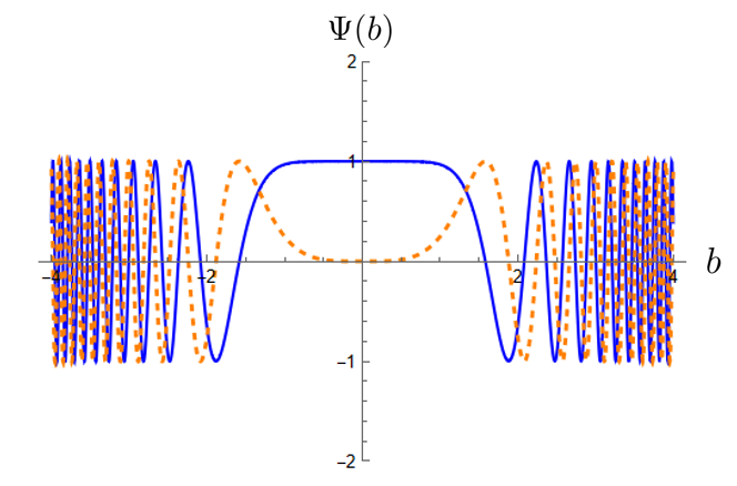
Figure 1: The real and imaginary parts of the minisuperspace wavefunction Eq. (29) (solid blue and dashed orange, respectively) for $c=0$.

It is difficult to make contact with the minisuperspace wavefunction derived in Magueijo et al. (2020) for the Pontryagin theory, because the wavefunction derived there always contains an admixture of Gauss-Bonnet contributions.

V Discussion

In quantizing the theories of GR and dCS with a cosmological constant $\Lambda$, the Pontryagin term that arises from dCS ($\theta R\tilde{R})$ yields a modification to the Kodama state from quantizing GR alone. The variation of the Chern-Simons coupling $\dot{\theta}$ can be directly related to $\dot{\Lambda}$. The full exact solution depends on the value of the three-curvature integrated over the connection space and the value of the Chern-Simons functional $Y_{\text{CS}}(A)$ integrated over the same space.
We can define a Chern-Simons time $\tau_{\text{CS}}=\int Y_{\text{CS}}(A)$ as in Alexander et al. (2018); Magueijo and Smolin (2018), where $\Lambda$ and $\tau_{\text{CS}}$ obey the commutation relations

$$[\hat{\Lambda},\hat{\tau}_{\text{CS}}]=i\frac{16\pi\Lambda^{2}}{3M_{P}^{2}},$$ (34)

or replacing $\Lambda$ with $\theta$,

$$\bigg{[}\hat{\theta},\hat{\tau}_{\text{CS}}\bigg{]}=i.$$ (35)

Furthermore, an uncertainty principle between $\Lambda$ and $\tau_{\text{CS}}$ can be derived:

$$\Delta\Lambda\Delta\tau_{\text{CS}}\geq\frac{4\pi}{3M_{P}^{2}}\langle\hat{\Lambda}\rangle^{2}.$$ (36)

From Eq. (36), we see that $\Lambda$ and $\tau_{\text{CS}}$ are incompatible with each other if $\langle\hat{\Lambda}\rangle$ is large (correspondingly, if $\langle\hat{\theta}\rangle$ is small). On the other hand, the cosmological constant and Chern-Simons time can be treated as classical variables if $\langle\hat{\Lambda}\rangle$ is small (i.e. $\langle\hat{\theta}\rangle$ is large) Alexander et al. (2018). This can be achieved by tuning the Chern-Simons coupling $\theta$ such that it is sufficiently small.

VI Summary and Outlook

We have found that the correction from dCS gravity directly allows for the variation of $\Lambda$, which makes our full modified Kodama state a strong candidate for describing quantum gravity non-perturbatively with a time-varying cosmological constant.
We close by noting that other classical methods for inducing a time variation in $\Lambda$ have been proposed, not always phenomenologically successful Alexander et al. (2019a, b); Magueijo and Złośnik (2019); Alexander et al. (2020). This early work, nonetheless, already points to a deep relation between a varying $\Lambda$ and the Pontryagin term, as well as Chern-Simons gravity. The relation with their metric representation cousins of these states Magueijo (2020), however, remains to be explored. One senses that the decades-long discussion about boundary conditions initiated by Hartle and Hawking Hartle and Hawking (1983) and Vilenkin Vilenkin (1998) could benefit from this radically different perspective.