From Infinity to Choreographies

Abstract

Choreographies are formal descriptions of distributed systems, which focus on the way in which participants communicate. While they are useful for analysing protocols, in practice systems are written directly by specifying each participant’s behaviour. This created the need for choreography extraction: the process of obtaining a choreography that faithfully describes the collective behaviour of all participants in a distributed protocol.

Previous works have addressed this problem for systems with a predefined, finite number of participants. In this work, we show how to extract choreographies from system descriptions where the total number of participants is unknown and unbounded, due to the ability of spawning new processes at runtime. This extension is challenging, since previous algorithms relied heavily on the set of possible states of the network during execution being finite.

1 Introduction

Choreographies are coordination plans for concurrent and distributed systems, which describe the expected interactions that system participants should enact [5, 13]. Languages for expressing choreographies (choreographic languages) are widely used for documentation and specification purposes, some notable examples being Message Sequence Charts [7], UML Sequence Diagrams [15], and choreographies in the Business Process Modelling Notation (BPMN) [14]. More recently, such languages have also been used for programming and verification, e.g., as in choreographic programming [12] and multiparty session types [6] respectively.

In practice, many system implementations do not come with a choreography yet. Choreography extraction (extraction for short) is the synthesis of a choreography that faithfully represents the specification of a system based on message passing (if it exists) [1, 3, 10, 11]. Extraction is helpful because it gives developers a global overview of how the processes (abstractions of endpoints) of a system interact, making it easier to check that they collaborate as intended. In general, though, it is undecidable whether such a choreography exists, making extraction a challenging problem.

Current methods for extraction cannot analyse systems that spawn new processes at runtime: they can only deal with systems where the number of participants is finite and statically known. This is an important limitation, because many modern distributed systems dynamically create processes for several reasons, such as scalability. The aim of this article is to address this shortcoming.

As an example of a system that cannot be analysed by previous work, consider a simple implementation of a serverless architecture (Example 1).

Example 1

A simple serverless architecture, written in pseudocode (we will formalise this example later in the article). A client sends a request to an entry-point, which then spawns a temporary process to handle the client. The spawned process computes the response to the request. Then it offers the client to make another request, in which case a new process is spawned to handle that, since the new request may require a different service.

⬇

client:

send init to server;

loop {

server presents worker; receive result from worker;

if finished

then request termination from worker; terminate;

else request next from worker; server:=worker;

}

server:

receive init from client; Handle(server);

procedure Handle(parent) {

spawn worker with {

parent presents client; ComputeResult();

send result to client; receive request from client;

switch request {

next: Handle(worker);

termination: terminate;

}

}

introduce worker and client; terminate;

}

Example 1 illustrates the usefulness of extraction: a human could manually go through the code and check that the two processes will interact as intended; however, despite it being a greatly simplified example, it is not immediately obvious whether the processes will communicate correctly or not.

Previous methods for extraction use graphs to represent the possible (symbolic) execution space of the system under consideration. The challenge presented by code as in Example 1 is that these graphs are not guaranteed to be finite anymore, because of the possibility of spawning new processes at runtime.

In this article we introduce the first method for extracting choreographies that supports process spawning, i.e., the capability of creating new processes at runtime. Our main contribution consists of a theory and implementation of extraction that use name substitutions to obtain finite representations of infinite symbolic execution graphs. Systems with process spawning have a dynamic topology, which further complicates extraction: new processes can appear at runtime, and can then be connected to other processes to enable communication. We extend the languages used for extraction in previous work with primitives for capturing these features, and show that our method can deal with them.

Structure of the paper.

In Section 2, we recap the basic theory of extraction. In Section 3, we introduce the languages for representing systems (as networks of processes) and choreographies. Section 4 reports our method for extracting networks with an unbounded number of processes (due to spawning), its implementation and limitations. We conclude in Section 5.

Related work.

We have already mentioned most of the relevant related work in this section. Choreography extraction has been explored for languages that include internal computation [3], process terms that correspond to proofs in linear logic [1], and session types (abstract terms without internal computation) [10, 11]. Our method deals with the first case (the most general among those cited). Our primitives for modelling process spawning are inspired by [4].

2 Background

This section summarizes the framework for choreography extraction that we extend [2, 3, 8, 16]. The remainder of the article expands upon this work to extend the capabilities of extraction, and to bring it closer to real systems.

2.1 Networks

Distributed systems are modelled as networks, which consist of several participants executing in parallel. Each participant is called a process, and the sequence of actions it executes is called a behaviour. Each process also includes a set of procedures, consisting of a name and associated behaviour.

Behaviours are formally defined by the grammar given below.

$$B::= \ \textbf{0}\mid X\mid\mathsf{p}!m;B\mid\mathsf{p}?;B\mid\mathsf{p}\oplus\ell;B\mid\mathsf{p}\&\{\ell_{1}:B_{1},\ldots,\ell_{n}:B_{n}\}$$

$$\mid\texttt{if }\!e\!\texttt{ then }\!B_{1}\texttt{ else }\!B_{2}$$

Term 0 designates a terminated process. Term $X$ invokes the procedure named X. Invoking a procedure must be the last action on a behaviour – in other words, we only allow tail recursion. Term $\mathsf{p}!m;B$ describes a behaviour where the executing process evaluates message $m$ and sends the corresponding value to process $\mathsf{p}$, then continues as $B$. The dual term $\mathsf{p}?;B$ describes receiving a message from $\mathsf{p}$, storing it locally and continuing as $B$. Behaviour $\mathsf{p}\oplus\ell;B$ sends the selection of label $\ell$ to process $\mathsf{p}$ then continues as $B$, while the dual $\mathsf{p}\&\{\ell_{1}:B_{1},\ldots,\ell_{n}:B_{n}\}$ offers the behaviours $B_{1},\ldots,B_{n}$ to $\mathsf{p}$, which can be selected by the corresponding labels $\ell_{1},\ldots,\ell_{n}$. Finally, $\texttt{if }e\texttt{ then }B_{1}\texttt{ else }B_{2}$ is the conditional term: if the Boolean expression $e$ evaluates to true, it continues as $B_{1}$, otherwise, it continues as $B_{2}$.

The syntax

⬇

$\mathsf{p}$ {

def $X_{1}$ { $B_{1}$ }

$\vdots$

def $X_{n}$ { $B_{n}$ }

main { $B$ }

}

describes a process named $\mathsf{p}$ with local procedures $X_{1},\ldots,X_{n}$ defined respectively as $B_{1},\ldots,B_{n}$, intending to execute behaviour $B$.

A network is specified as a sequence of processes, all with distinct names, separated by vertical bars (|). Example 2 defines a valid network, which we use as running example throughout this section to explain the existing extraction algorithm.

Example 2

This network describes the protocol for an online store. The customer sends in items to purchase, then asks the store to proceed to checkout, or continue browsing.

Once the customer proceeds to checkout, they send their payment information to the store. The store then verifies that information, and either completes the transaction, or asks the client to re-send payment information if there where a problem.

⬇

$\mathsf{customer}$ {

def $\mathit{browse}${ $\mathsf{store}$!$\mathit{item}$; if $\mathit{checkout}$

then $\mathsf{store}$$\oplus\mathit{buy}$; $\mathit{purchase}$;

else $\mathsf{store}$$\oplus\mathit{more}$; $\mathit{browse}$ }

def $\mathit{purchase}${ $\mathsf{store}$!$\mathit{payment}$; $\mathsf{store}$&{$\mathit{accept}$: 0, $\mathit{reject}$: $\mathit{purchase}$} }

main{ $\mathit{browse}$ }

} |

$\mathsf{store}$ {

def $\mathit{offer}${ $\mathsf{customer}$?; $\mathsf{customer}$&{$\mathit{buy}$: $\mathit{payment}$, $\mathit{more}$: $\mathit{offer}$} }

def $\mathit{payment}${ $\mathsf{customer}$?; if $\mathit{accepted}$

then $\mathsf{customer}$$\oplus\mathit{accept}$; 0

else $\mathsf{customer}$$\oplus\mathit{reject}$; $\mathit{payment}$ }

main { $\mathit{offer}$ }

}

2.2 Choreographies

Global descriptions of distributed systems, specifying interactions between participants rather than their individual actions, are called choreographies. Similar to processes in networks, a choreography contains a set of procedure definitions, and a main body. The terms of choreography bodies are defined by the grammar below and closely correspond to the actions in process behaviours.

$$C::= \ \textbf{0}\mid X\mid\mathsf{p}.m\,\mbox{\tt{-\!\raisebox{-0.51663pt}{>}}}\,\mathsf{q};C\mid\mathsf{p}\,\mbox{\tt{-\!\raisebox{-0.51663pt}{>}}}\,\mathsf{q}[\ell];C\mid\texttt{if }\mathsf{p}.e\texttt{ then }C_{1}\texttt{ else }C_{2}$$

Term 0 denotes a choreography body where all processes are terminated. Term $X$ invokes the procedure with name X. In the communication $\mathsf{p}.m\,\mbox{\tt{-\!\raisebox{-0.51663pt}{>}}}\,\mathsf{q};C$, process $\mathsf{p}$ sends message $m$ to $\mathsf{q}$, which stores the result, and the system continues as described by choreography body $C$. Likewise, in label selection $\mathsf{p}\,\mbox{\tt{-\!\raisebox{-0.51663pt}{>}}}\,\mathsf{q}[\ell];C$, process $\mathsf{p}$ selects an action in $\mathsf{q}$ by sending the label $\ell$, and the system continues as $C$. In the conditional $\texttt{if }\mathsf{p}.e\texttt{ then }C_{1}\texttt{ else }C_{2}$, process $\mathsf{p}$ starts by evaluating the Boolean expression $e$; if this resolves to true, then the choreography continues as $C_{1}$, otherwise it continues as $C_{2}$.

Example 3

The protocol described by the network in Example 2 can be written as the following choreography.

⬇

def $\mathit{Buy}$ {

$\mathsf{customer}$.$item$ -​> $\mathsf{store}$; if $\mathsf{customer}$.$checkout$

then $\mathsf{customer}$ -​> $\mathsf{store}$$[buy]$; $\mathit{Pay}$

else $\mathsf{customer}$ -​> $\mathsf{store}$$[more]$; $\mathit{Buy}$

}

def $\mathit{Pay}$ {

$\mathsf{customer}$.$\mathit{payment}$ -​> $\mathsf{store}$; if $\mathsf{store}$.$\mathit{accepted}$

then $\mathsf{store}$ -​> $\mathsf{customer}$$[accept]$; 0

else $\mathsf{store}$ -​> $\mathsf{customer}$$[reject]$; $\mathit{Pay}$

}

main {$\mathit{Buy}$}

2.3 Extraction algorithm

The extraction algorithm from [2, 3] consists of two steps. The first step is building a graph that represents a symbolic execution of the network. The second is to traverse this graph, using its edges to build the extracted choreography.

2.3.1 Graph generation.

The first step in extracting a choreography from a network is building a Symbolic Execution Graph (SEG) from the network. A SEG is a directed graph representing an abstraction of the possible evolutions of the network over time. It abstracts from the concrete semantics by ignoring the concrete values being communicated and considering both possible outcomes for every conditional. Nodes contain possible states of the network, and edges connect nodes that are related by execution of one action (the label of the edge).

Edges in the SEG are labeled by transition labels, which represent the possible actions executable by the network: value communications (matching a send action with the corresponding receive), label selection (matching selection and offer), and conditionals. For the last there are two labels, representing the two possible outcomes (the “then” and “else” branch, respectively).

$$\lambda::=\mathsf{p}.e\,\mbox{\tt{-\!\raisebox{-0.51663pt}{>}}}\,\mathsf{q}\mid\mathsf{p}\,\mbox{\tt{-\!\raisebox{-0.51663pt}{>}}}\,\mathsf{q}[\ell]\mid\mathsf{p}.e\texttt{ then}\mid\mathsf{p}.e\texttt{ else}$$

As an example, we show how to build the SEG for the network in Example 2 (see Fig. 1). The main behaviours of the two processes are procedure invocations (node on top). Expanding the corresponding definitions, we find out that the first action by $\mathsf{customer}$ is sending to $\mathsf{store}$, while $\mathsf{store}$’s first action is receiving from $\mathsf{customer}$. These actions match, so the network can execute an action reducing both $\mathsf{store}$ and $\mathsf{customer}$. This results in a new network, which is placed in a new node, and we connect both nodes by the transition label describing the executed action.

The next action by $\mathsf{customer}$ is receiving a label from $\mathsf{store}$, but $\mathsf{store}$ needs to evaluate a conditional expression to decide which label to send. There are two possible outcomes for these evaluation, so we create two new nodes and label the edges towards them with the corresponding possibilities (then or else). Continuing to expand the else branch leads to a network that is already in the SEG, so we simply add an edge to the node containing that network. The then branch evolves in two steps into a second conditional, whose else branch again creates a loop, while its then branch evolves into a network where all processes has terminated. This concludes the construction of the SEG.

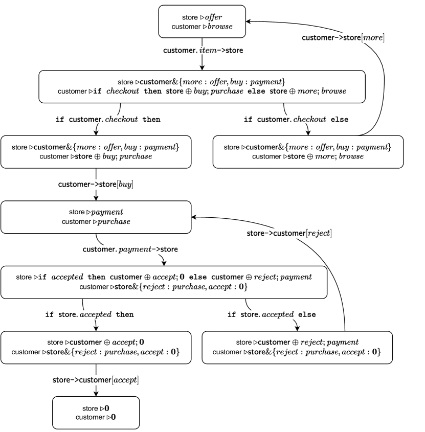
Figure 1: The SEG of the network from Example 2.

In this example SEG generation went flawlessly, but that is not always the case. We saw that a process trying to send a message must wait for the receiving process to be able to execute a matching receive; this can lead to situations where the network is deadlocked – no terms can be executed. In that case, the behaviour of the network cannot be described by a choreography, and the network cannot be extracted.

This algorithm also relies on the fact that network execution is confluent: the success of extraction does not depend on which action is chosen when constructing the SEG, in case several are possible. (This can affect the algorithm’s performance, though.) Furthermore, guaranteeing that all possible evolutions of the network are captured requires some care when closing loops: all processes must reduce in every cycle in the SEG. This is achieved by marking processes in the network and checking that every loop contains a node where all processes are marked. These aspects are orthogonal to the current development, and we refer the interested reader to [3] for details.

2.3.2 Choreography construction.

The main idea for generating a choreography from a SEG is that edges correspond to choreography actions, so the choreography essentially describes all paths in the SEG. The choreographic way of representing loops is by means of procedures, so each loop in the SEG should become a procedure definition. To achieve this, we first unroll the graph by splitting every loop node – the nodes that close a loop – into two: a exit node, which is the target of all edges previously pointing to the loop node, and a entry node, which is the source of all edges previously pointing from the loop node. Entry nodes are given distinct procedure names, and exit nodes are associated with the corresponding procedure calls. The unrolled SEG is now a forest with each tree representing a procedure, as shown in Fig. 2.

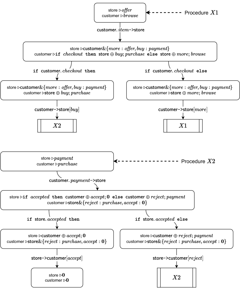
Figure 2: The unrolling of the graph of Fig. 1 resulting in two trees, each corresponding to a procedure in the SEG to be extracted. For readibility, the exit node corresponding to the invocation of $X2$ is depicted twice.

Since transition labels are similar to the choreography body terms, it is simple to read choreography bodies directly from each tree of the unrolled graph. This is done recursively, starting from the root of each tree and proceeding as follows: when encountering a node with no outgoing edges, then either all processes have terminated, in which case we return 0, or the node is an exit node, in which case we return the corresponding procedure invocation. If there is one outgoing edge, that edge represents an interaction, so we return the choreography body that starts with the transition label for that edge and continues as the result of the recursive invocation on the edge’s target. If there are two outgoing edges, then we return a conditional choreography body whose two continuations are the results of the recursive calls targets of the two edges, as dictated by those edges’ labels.

Example 4

By reading the trees in Fig. 2 in the manner described, we obtain the choreography given earlier in Example 3, where procedures $Buy$ and $Pay$ are now called $X1$ and $X2$, respectively.

3 Networks and Choreographies with Process Spawning

In this section, we extend the theories of networks and choreographies with support for spawning new processes at runtime.

We start by adding three primitives to the language of behaviours, following ideas from [4].

1. Spawning of processes. The language of behaviours is extended with the construct $\texttt{spawn }\mathsf{q}\texttt{ with }B_{\mathsf{q}}\texttt{ continue }B$, which adds a new process to the network with a new, unique name. The new process gets main behaviour $B_{\mathsf{q}}$, and inherits its parent’s set of procedures, while the parent continues executing $B$. This term also binds $\mathsf{q}$ (a process variable) in $B$.

2. Advertising processes. Since names of newly spawned processes are only known to their parents, we need terms for communicating process names. Process $\mathsf{p}$ can “introduce” $\mathsf{q}$ and $\mathsf{r}$ to each other (send each of them the other’s name) by executing term $\mathsf{q}\,\mbox{\tt{\raisebox{-0.51663pt}{<}\!-\!\raisebox{-0.51663pt}{>}}}\,\mathsf{r};B$, while $\mathsf{q}$ and $\mathsf{r}$ execute the dual actions $\mathsf{p}?\mathsf{t};\;B_{\mathsf{q}}$ and $\mathsf{p}?\mathsf{t};\;B_{\mathsf{r}}$. Here $\mathsf{t}$ is again a variable, which is bound in the continuations $B_{\mathsf{q}}$ and $B_{\mathsf{r}}$.

3. Parameterised procedures. To be able to use processes spawned at runtime in procedures, their syntax is changed so that they can take process names as parameters.

We do not distinguish process names from process variables syntactically, as this simplifies the semantics. We assume as usual that all binders in the same term bind distinct variables, and work up to $\alpha$-renaming. However, we allow a variable to occur both free and bound in the same term – this is essential for our algorithm.

As previously, the semantics includes a state function $\sigma$, mapping each process to a value (its memory state). The new ingredient is a graph of connections $\mathcal{G}$ between processes, connecting pairs of process that are allowed to communicate. The choice of the initial graph allows for modelling different network topologies. We use the notation $\mathsf{p}\leftrightarrow\mathsf{q}\in\mathcal{G}$ to denote that $\mathsf{p}$ and $\mathsf{q}$ are connected in $\mathcal{G}$, and $\mathcal{G}\cup\{\mathsf{p}\leftrightarrow\mathsf{q}\}$ to denote the graph obtained from $\mathcal{G}$ by adding an edge between $\mathsf{p}$ and $\mathsf{q}$.

Fig. 3 includes some representative rules of this extended semantics.

$$\mathsf{p}\leftrightarrow\mathsf{q}\in\mathcal{G} e\downarrow^{\sigma}_{\mathsf{p}}v \mathsf{p}\triangleright\mathsf{q}!e;B_{1}\mid\mathsf{q}\triangleright\mathsf{p}?;B_{2},\sigma,\mathcal{G}\xrightarrow[]{\mathsf{p}.v\,\mbox{\tt{-\!\raisebox{-0.51663pt}{>}}}\,\mathsf{q}}\mathsf{p}\triangleright B_{1}\mid\mathsf{q}\triangleright B_{2},\sigma[\mathsf{q}\mapsto v],\mathcal{G}$$      N|Com

$$\mathsf{p}\leftrightarrow\mathsf{q}\in\mathcal{G} \mathsf{p}\leftrightarrow\mathsf{r}\in\mathcal{G} \begin{array}[]{c}\mathsf{p}\triangleright\mathsf{q}\,\mbox{\tt{\raisebox{-0.51663pt}{<}\!-\!\raisebox{-0.51663pt}{>}}}\,\mathsf{r};B_{\mathsf{p}}\mid\mathsf{q}\triangleright\mathsf{p}?\mathsf{r};B_{\mathsf{q}}\mid\mathsf{r}\triangleright\mathsf{p}?\mathsf{q};B_{\mathsf{r}},\sigma,\mathcal{G}\\ \xrightarrow[]{\mathsf{p}.\mathsf{q}\,\mbox{\tt{\raisebox{-0.51663pt}{<}\!-\!\raisebox{-0.51663pt}{>}}}\,\mathsf{r}}\\ \mathsf{p}\triangleright B_{\mathsf{p}}\mid\mathsf{q}\triangleright B_{\mathsf{q}}\mid\mathsf{r}\triangleright B_{\mathsf{r}},\sigma,\mathcal{G}\cup\{\mathsf{q}\leftrightarrow\mathsf{r}\}\end{array}$$      N|Intro

  $$\begin{array}[]{c}\mathsf{p}\triangleright\texttt{spawn $\mathsf{q}$ with $B_{q}$ continue $B$},\sigma,\mathcal{G}\\ \xrightarrow[]{\mathsf{p}\texttt{ spawns }\mathsf{q}}\\ \mathsf{p}\triangleright B\mid\mathsf{q}\triangleright B_{q},\sigma,\mathcal{G}\cup\{\mathsf{p}\leftrightarrow\mathsf{q}\}\end{array}$$ N|Spawn

Figure 3: New semantics of networks, selected rules.

Rule N|Com describes a communication. Process $\mathsf{p}$ wants to send the result of evaluating $e$ to process $\mathsf{q}$, and $\mathsf{q}$ is expecting to receive from $\mathsf{p}$. These processes can communicate, and the result $v$ of evaluating $e$ at $\mathsf{p}$ is sent and stored in $\mathsf{q}$ (premise $e\downarrow^{\sigma}_{\mathsf{p}}v$). The difference from the previous semantics is the presence of the additional premise $\mathsf{p}\leftrightarrow\mathsf{q}\in\mathcal{G}$, which checks that these two processes are allowed to communicate.

Rule N|Intro is similar, but process names are communicated instead, and the communication graph is updated. For simplicity, instead of explicitly substituting variables for process names, we assume that the behaviours of $\mathsf{q}$ and $\mathsf{r}$ have previous been $\alpha$-renamed appropriately (this kind of simplifications based on $\alpha$-renaming are standard in process calculi [17]).

Rule N|Spawn creates a new process $\mathsf{q}$ into the network with a unique name, and adds an edge between it and its parent to the network. Note that $\mathsf{q}$ is distinct from other process names in the network.

Choreographies get two corresponding actions: $\texttt{$\mathsf{p}$ spawns $\mathsf{q}$};\;C$ and $\mathsf{p.q}\,\mbox{\tt{\raisebox{-0.51663pt}{<}\!-\!\raisebox{-0.51663pt}{>}}}\,\mathsf{r};\;C$. Procedures also become parameterized. At the choreography level we do not require process variables except in procedure definitions (which are replaced by process names when called); we assume that all names of spawned processes are unique (again treating spawn actions as binders and $\alpha$-renaming in procedure bodies when needed at invocation time).

The corresponding rules for the semantics are given in Fig. 4.

$$\mathsf{p}\leftrightarrow\mathsf{q}\in\mathcal{G} e\downarrow^{\sigma}_{\mathsf{p}}v \mathsf{p}.e\,\mbox{\tt{-\!\raisebox{-0.51663pt}{>}}}\,\mathsf{q};C,\sigma,\mathcal{G}\xrightarrow[]{\mathsf{p}.v\,\mbox{\tt{-\!\raisebox{-0.51663pt}{>}}}\,\mathsf{q}}C,\sigma[\mathsf{q}\mapsto v],\mathcal{G}$$      C|Com

$$\mathsf{p}\leftrightarrow\mathsf{q}\in\mathcal{G} \mathsf{p}\leftrightarrow\mathsf{r}\in\mathcal{G} \mathsf{p}.\mathsf{q}\,\mbox{\tt{\raisebox{-0.51663pt}{<}\!-\!\raisebox{-0.51663pt}{>}}}\,\mathsf{r};C,\sigma,\mathcal{G}\xrightarrow[]{\mathsf{p}.\mathsf{q}\,\mbox{\tt{\raisebox{-0.51663pt}{<}\!-\!\raisebox{-0.51663pt}{>}}}\,\mathsf{r}}C,\sigma,\mathcal{G}\cup\{\mathsf{q}\leftrightarrow\mathsf{r}\}$$      C|Intro

  $$\mathsf{p}\texttt{ spawns }\mathsf{q};C,\sigma,\mathcal{G}\xrightarrow[]{\mathsf{p}\texttt{ spawns }\mathsf{q}}C,\sigma,\mathcal{G}\cup\{\mathsf{p}\leftrightarrow\mathsf{q}\}$$ C|Spawn

Figure 4: New semantics of choreographies, selected rules.

Example 5

We illustrate a network with process spawning by writing Example 1 in our language. The client sends a request to an entry-point, which then spawns an instance to handle the request, which gets introduced to the client. The instance sends the client the result, and the client either makes another request or terminates the connection. Additional requests spawn new instances, since requests may differ in kind – this is handled by the previous instance to reduce load on the entry-point.

⬇

$\mathsf{client}$ {

def $X$(s){

$\mathsf{s}$?$\mathsf{w}$; $\mathsf{w}$?; if $\mathit{more}$

then $\mathsf{w}$$\oplus next$; $X$($\mathsf{w}$)

else $\mathsf{w}$$\oplus end$; 0

}

main{ $\mathsf{entry}$!$req$; $X$($\mathsf{entry}$) }

}

⬇

| $\mathsf{entry}$ {

def $X$($\mathsf{this}$){

spawn $\mathsf{worker}$ with

$\mathsf{this}$?$\mathsf{client}$; $\mathsf{client}$!$res$; $\mathsf{client}$&{ $next$: $X$($\mathsf{worker}$), $end$: 0 }

continue $\mathsf{worker}$ <​-​> $\mathsf{client}$; 0

}

main{ $\mathsf{client}$?; $X$($\mathsf{entry}$) }

}

After the initial communication and procedure call, variable $\mathsf{w}$ in $\mathsf{client}$ needs to be renamed to $\mathsf{worker}$ in order for the next communication to reduce.

4 Extraction with process spawning

In the presence of spawning, the intuitive process of extraction described earlier no longer works: since a network can generate an unbounded number of new processes, there is no guarantee that the SEG is finite and, as a consequence, that the procedure terminates.

However, we observe that since networks are finite and can only reduce to networks built from their subterms, there is only a finite number of possible behaviours for processes that are spawned at runtime. Therefore we can keep SEGs finite if we allow renaming processes when connecting nodes. This intuition is key to our development.

Example 6

Consider the network from Example 5 and its SEG, shown in Fig. 5. The dotted part shows the network that would be generated by symbolic execution as described earlier. By allowing renaming of processes, we can close a loop by applying the mapping $\{\mathsf{client}\mapsto\mathsf{client},\mathsf{entry/worker0}\mapsto\mathsf{entry}\}$. The parameters $\mathsf{w}$ and $\mathsf{worker}$ are both variables mapping to $\mathsf{entry/worker0}$, and since $\mathsf{entry}$ has terminated, the remapping makes the dotted node equivalent to the second node of the SEG, as shown by the loop. For simplicity we only show the process variables that are changed by the mapping, i.e., we omit $\mathsf{client}\mapsto\mathsf{client}$.

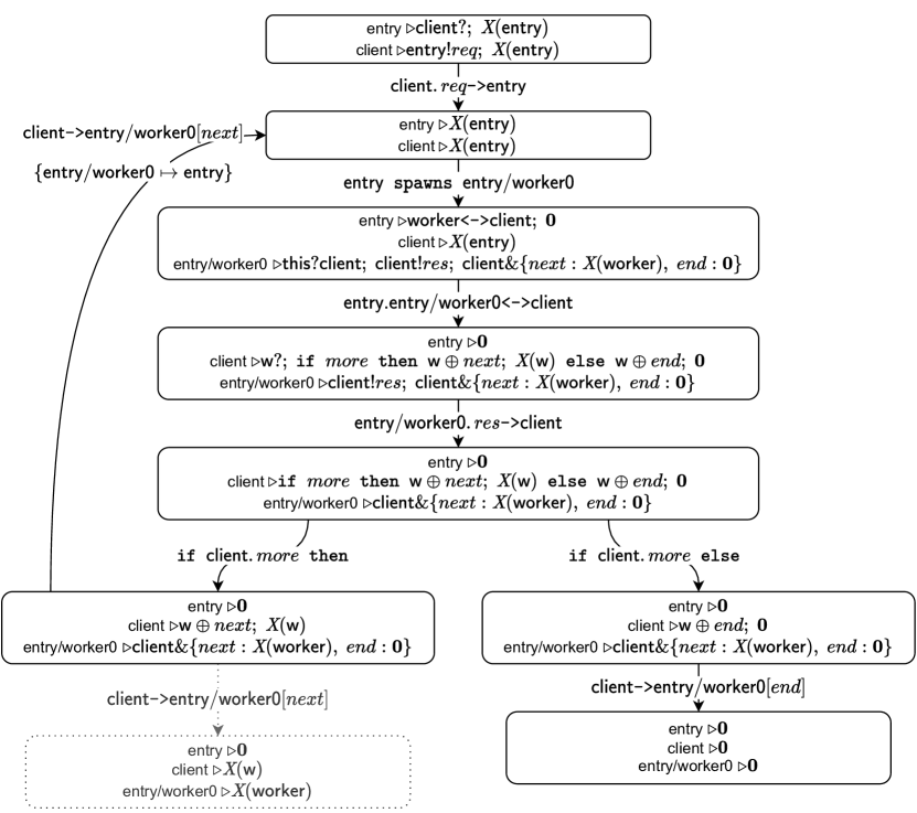
Figure 5: The SEG of the network in Example 5.

4.1 Generating SEGs

Formally, we define an abstract semantics for networks that makes two changes with respect to the concrete semantics given above. First, we remove all information about states $\sigma$ (and as a consequence about the actual values being communicated), as in [2]. Secondly, we now treat all process names as variables, and replace the communication graph $\mathcal{G}$ by a partial function $\gamma$ mapping pairs of a process name and a process variable to process names: intuitively, $\gamma(\mathsf{p},\mathsf{q})$ returns the name of the actual process that $\mathsf{p}$ locally identifies as $\mathsf{q}$. If $\gamma(\mathsf{p},\mathsf{q})$ is undefined, then $\mathsf{p}$ does not know who to communicate with. We assume that initially $\gamma(\mathsf{p},\mathsf{p})=\mathsf{p}$ for all $\mathsf{p}$, and that, for all $\mathsf{p}$ and $\mathsf{q}$, either $\gamma(\mathsf{p},\mathsf{q})=\mathsf{q}$ (meaning that $\mathsf{p}$ knows $\mathsf{q}$’s name and is allowed to communicate with it) or $\gamma(\mathsf{p},\mathsf{q})$ is undefined (meaning that $\mathsf{p}$ is not connected to $\mathsf{q}$ and cannot communicate with it) – this allows us to model different initial network topologies. Fig. 6 shows the abstract versions of the rules previously shown.

$$\mathsf{r}\downarrow^{\gamma}_{\mathsf{p}}\mathsf{q}\quad\mathsf{s}\downarrow^{\gamma}_{\mathsf{q}}\mathsf{p} \mathsf{p}\triangleright\mathsf{r}!e;B_{1}\mid\mathsf{q}\triangleright\mathsf{s}?;B_{2},\gamma\xrightarrow[]{\mathsf{p}.e\,\mbox{\tt{-\!\raisebox{-0.51663pt}{>}}}\,\mathsf{q}}\mathsf{p}\triangleright B_{1}\mid\mathsf{q}\triangleright B_{2},\gamma$$   N|Com

$$\mathsf{s}\downarrow^{\gamma}_{\mathsf{p}}\mathsf{q}\quad\mathsf{t}\downarrow^{\gamma}_{\mathsf{p}}\mathsf{r}\quad\mathsf{u}\downarrow^{\gamma}_{\mathsf{q}}\mathsf{p}\quad\mathsf{v}\downarrow^{\gamma}_{\mathsf{r}}\mathsf{p} \begin{array}[]{c}\mathsf{p}\triangleright\mathsf{s}\,\mbox{\tt{\raisebox{-0.51663pt}{<}\!-\!\raisebox{-0.51663pt}{>}}}\,\mathsf{t};B_{\mathsf{p}}\mid\mathsf{q}\triangleright\mathsf{u}?\mathsf{w};B_{\mathsf{q}}\mid\mathsf{r}\triangleright\mathsf{v}?\mathsf{x};B_{\mathsf{r}},\gamma\\ \xrightarrow[]{\mathsf{p}.\mathsf{q}\,\mbox{\tt{\raisebox{-0.51663pt}{<}\!-\!\raisebox{-0.51663pt}{>}}}\,\mathsf{r}}\\ \mathsf{p}\triangleright B_{\mathsf{p}}\mid\mathsf{q}\triangleright B_{\mathsf{q}}\mid\mathsf{r}\triangleright B_{\mathsf{r}},\gamma[\langle\mathsf{q,w}\rangle\mapsto\mathsf{r}][\langle\mathsf{r,x}\rangle\mapsto\mathsf{u}]\end{array}$$   N|Intro

  $$\begin{array}[]{c}\mathsf{p}\triangleright\texttt{spawn $\mathsf{q}$ with $B_{q}$ continue $B$},\gamma\\ \xrightarrow[]{\mathsf{p}\texttt{ spawns }\mathsf{q}}\\ \mathsf{p}\triangleright B\mid\mathsf{r}\triangleright B_{q},\gamma[\langle\mathsf{p,q}\rangle\mapsto\mathsf{r}][\langle\mathsf{r,p}\rangle\mapsto\mathsf{p}]\end{array}$$ N|Spawn

Figure 6: Abstract semantics of networks, selected rules

Example 7

It is easy to check that the SEG shown in Fig. 5 follows the rules in Fig. 6. Initially, the variable mapping is the identity, and this remains unchanged after the first communication.

$\gamma$	$\mathsf{entry}$	$\mathsf{client}$	$\mathsf{worker}$	$\mathsf{w}$
$\mathsf{entry}$	$\mathsf{entry}$	$\mathsf{client}$	—	—
$\mathsf{client}$	$\mathsf{entry}$	$\mathsf{client}$	—	—

When $\mathsf{entry}$ spawns the new process $\mathsf{entry/worker0}$, this name is associated to $\mathsf{entry}$’s local variable $\mathsf{worker}$ according to rule N|Spawn. So the variable mapping is now given by the following table.

$\gamma$	$\mathsf{entry}$	$\mathsf{client}$	$\mathsf{worker}$	$\mathsf{w}$
$\mathsf{entry}$	$\mathsf{entry}$	$\mathsf{client}$	$\mathsf{entry/worker0}$	—
$\mathsf{client}$	$\mathsf{entry}$	$\mathsf{client}$	—	—
$\mathsf{entry/worker0}$	$\mathsf{entry}$	—	—	—

Next, $\mathsf{entry}$ introduces $\mathsf{entry/worker0}$ and $\mathsf{client}$ to each other; $\mathsf{client}$ uses the local name $\mathsf{w}$ for the new process. According to rule N|Intro, the variable mapping is now the following.

$\gamma$	$\mathsf{entry}$	$\mathsf{client}$	$\mathsf{worker}$	$\mathsf{w}$
$\mathsf{entry}$	$\mathsf{entry}$	$\mathsf{client}$	$\mathsf{entry/worker0}$	—
$\mathsf{client}$	$\mathsf{entry}$	$\mathsf{client}$	—	$\mathsf{entry/worker0}$
$\mathsf{entry/worker0}$	$\mathsf{entry}$	$\mathsf{client}$	—	—

To determine whether we can close a loop in the SEG, we need the following definitions.

Definition 1

Two networks $N$ and $N^{\prime}$ are equivalent if there exists a total bijective mapping $M$ from processes in $N$ to processes in $N^{\prime}$, such that, for all processes $\mathsf{p}$:

• if $\mathsf{p}$ has main behaviour $B$, then $M(\mathsf{p})$ has main behaviour $M(B)$ (where $M$ is extended homeomorphically to behaviours);

• if $\mathsf{p}$ has not terminated and $X(\tilde{\mathsf{q}})=B$ is a procedure definition in $\mathsf{p}$, then $X=M_{\mathsf{q}}(B)$ is a procedure definition in $M(\mathsf{p})$, where $M_{\mathsf{q}}$ maps every process in $\tilde{\mathsf{q}}$ to itself and every other process $\mathsf{r}$ to $M(\mathsf{r})$.

To close a loop in the SEG, we also need to look at the variable mappings $\gamma$.

Definition 2

Two nodes $N,\gamma$ and $N^{\prime},\gamma^{\prime}$ in a SEG are behaviourally equivalent if:

• There exists a series of reductions $\tilde{\lambda}$ in the SEG such that $N,\gamma\xrightarrow[]{\tilde{\lambda}}^{*}N^{\prime},\gamma^{\prime}$;

• There exists a mapping function $M$ that proves $N$ and $N^{\prime}$ are equivalent.

• If $M(\mathsf{p})=\mathsf{q}$, $\gamma(\mathsf{p,a})=\mathsf{b}$, $\gamma^{\prime}(\mathsf{q,a})=\mathsf{c}$, and there is a reduction accessible from $N,\gamma$ that evaluates $\gamma^{*}(\mathsf{p,a})$ for some intermediary $\gamma^{*}$, then $M(\mathsf{b})=\mathsf{c}$.

The last point of the definition only applies to variables actually evaluated in reductions of $N$. This makes extraction more efficient (as more nodes are equivalent): a variable might have been used for a previous step in the evolution up to $N,\sigma$, but if it remains unused thereafter it does not affect the behaviour anymore, and can be ignored.

Lemma 1

Let $N,\gamma$ and $N^{\prime},\gamma^{\prime}$ be behaviourally equivalent nodes in a SEG for a given network. The graph obtained by redirecting all edges coming into $N^{\prime},\gamma^{\prime}$ to $N,\gamma$ and removing the nodes that are no longer accessible from the root is also a SEG for the original network.

Our implementation simply looks for a suitable $N,\gamma$ when $N^{\prime},\gamma^{\prime}$ is generated, and records the mapping $M$ in the edge leading to $N,\gamma$.

4.1.1 Detecting unrestricted spawning.

It is possible to create a network where processes are spawned in a loop, faster than they terminate, making the number of processes increase for every iteration. Such networks embody a resource leak, and they cannot be extracted by our theory. To ensure termination, our algorithm must be able to detect resource leaks, which is an undecidable problem. We deal with it as follows: when a new candidate node is generated, we check whether there is a surjective mapping with the properties described above such that there are at least two process values mapped to the same process name. If this happens, the algorithm returns failure. We include some examples of networks with resource leaks in Section 0.A.5.

4.2 Generating the choreography

Building a choreography from a SEG is similar to the original case. The main change deals with procedure calls: we use the variable mappings in edges that close loops to determine their parameters and arguments.

When unrolling the SEG, each node corresponding to a procedure definition gets a list of parameters corresponding to the process names that appear in the co-domain of any variable mapping in an edge leading to that node. Each procedure call is then appended to the reverse images of these processes by the mapping in the edge leading to it. Note that the edges do not contain process names that are mapped to themselves; as such, processes that are the same in all maps will not appear as arguments to the extracted procedure. A consequence of this is that some procedures may get an empty set of arguments.

After this transformation the choreography can again be extracted by recursively traversing the resulting forest.

We formulate the correctness of our extraction procedure in terms of strong bisimilarity [18].

Theorem 4.1

If $C$ is a choreography extracted from a network $N$, then $C\sim N$.

Example 8

We return to the network in Example 5, whose SEG was shown in Fig. 5. The only loop node has two incoming edges, one with empty (identity) mapping and another with $\{\mathsf{entry/worker0}\mapsto\mathsf{entry}\}$. Therefore this node is extracted to a procedure $X1$ with one process variable $\mathsf{entry}$. The original call simply instantiates this parameter as itself, while the recursive call replaces it with $\mathsf{entry/worker0}$.

The choreography extracted from this SEG is thus the following.

⬇

def $X1$($\mathsf{entry}$) {

$\mathsf{entry}$ spawns $\mathsf{entry/worker0}$; $\mathsf{entry.entry/worker0}$ <​-​> $\mathsf{client}$;

$\mathsf{entry/worker0}$.$res\,\mbox{\tt{-\!\raisebox{-0.46497pt}{>}}}\,$$\mathsf{client}$;

if $\mathsf{client}$.$\mathit{more}$

then $\mathsf{client}$ -​> $\mathsf{entry/worker0}$$[next]$; $X1$($\mathsf{entry/worker0}$)

else $\mathsf{client}$ -​> $\mathsf{entry/worker0}$$[end]$; 0

}

main { $\mathsf{client}$.$req\,\mbox{\tt{-\!\raisebox{-0.46497pt}{>}}}\,$$\mathsf{entry}$; $X1$($\mathsf{entry}$) }

4.3 Implementation and limitations

The extension of the original extraction algorithm to networks with process spawning has been implemented in Java. It can successfully extract the networks in the examples given here, as well as a number of randomly generated tests following the ideas from [3]. Due to space constraints, we do not report on the details of our testing strategy, which is an extension of the strategy presented in detail in [3], extended in the natural way to include networks with process spawning and introduction.

Since our language only allows for tail recursion, divide-and-conquer algorithms such as mergesort are currently still not extractable, and our next plan is to extend the algorithm to deal with general recursion. This is not a straightforward extension, as our way of constructing the SEG has no way of getting past a potentially infinite recursive subterm to its continuation.

Another example of an unextractable network, which does not use general recusion, is the following.

⬇

$\mathsf{s}$ {

def $X$($\mathsf{p,t}$){

if $cont$ then spawn $\mathsf{q}$ with $X$($\mathsf{t,q}$) continue $\mathsf{q}$?; $\mathsf{p}$!$m$; 0 else $\mathsf{p}$!$m$; 0

}

main{ $X$($\mathsf{p,s}$) }

} |

p{s?; stop}

Although the spawned processes behave as their parent, the entire network never repeats itself, and extraction fails: extracting a choreography would require closing a loop where some processes did not reduce. This is essentially the same limitation already discussed in [3], and cannot be avoided: given that the problem of determining whether a network can be represented by a choreography is in general undecidable [2], soundness of our algorithm implies that such networks will always exist.

5 Conclusion

We showed how the state-of-the-art algorithm for choreography extraction [2, 3] could be extended to accommodate for networks with process spawning. This adaptation requires allowing processes names to change dynamically, so that the total number of networks that needs to be consider remains finite. The resulting theory captures examples including loops where processes that are spawned at runtime take over for other processes that terminate in the meantime. This extension also required adding parameterised procedures to the network and choreography language, and including a form of resource leak detection to ensure termination.

A working implementation of choreography extraction with process spawning is available at [9].

Acknowledgements.

This work was partially supported by Villum Fonden, grant no. 29518.

Appendix 0.A Full definitions and proofs

For completeness, we include the full definitions of network and choreography semantics, as well as the proofs of our main results.

0.A.1 Networks

Behaviours are defined by the following grammar.

$$B::= \ \textbf{0}\mid X\mid\mathsf{p}!m;B\mid\mathsf{p}?;B\mid\mathsf{p}\oplus\ell;B\mid\mathsf{p}\&\{\ell_{1}:B_{1},\ldots,\ell_{n}:B_{n}\}$$

$$\mid\mathsf{q}\,\mbox{\tt{\raisebox{-0.51663pt}{<}\!-\!\raisebox{-0.51663pt}{>}}}\,\mathsf{r};B \mid\mathsf{p}?\mathsf{t};\;B_{\mathsf{q}}\mid\texttt{if }\!e\!\texttt{ then }\!B_{1}\texttt{ else }\!B_{2}\mid\texttt{spawn }\mathsf{q}\texttt{ with }B_{\mathsf{q}}\texttt{ continue }B$$

A process consists of a set of procedure definitions $\mathcal{D}_{\mathsf{p}}$ together with a (main) behaviour $B$, also written $\mathsf{p}\triangleright\{\texttt{def }X_{i}(\tilde{\mathsf{p}})=B_{i}\}_{i\in I}\texttt{ in }B$. A network is a finite set of processes running in parallel, together with a state $\sigma$ mapping pairs of a process name and variable name to the process’s variable’s value, and an undirected graph $\mathcal{G}$ whose nodes are the names of the processes in the network.

We use the following notations:

• $\sigma[\langle\mathsf{p},x\rangle\mapsto v]$ denotes the update of $\sigma$ where $\mathsf{p}$’s variable $x$ now maps to value $v$;

• $e\downarrow^{\sigma}_{\mathsf{p}}v$ denotes evaluating expression $e$ at process $\mathsf{p}$ under state $\sigma$ reduces to value $v$;

• $\mathsf{p}\leftrightarrow\mathsf{q}\in\mathcal{G}$ denotes that there is an edge between $\mathsf{p}$ and $\mathsf{q}$ in $\mathcal{G}$;

• $\mathcal{G}\cup\{\mathsf{p}\leftrightarrow\mathsf{q}\}$ denotes the graph obtained from $\mathcal{G}$ by adding an edge between $\mathsf{p}$ and $\mathsf{q}$.

The semantics of networks is given in form of transitions $N,\sigma,\mathcal{G}\xrightarrow[]{\lambda}N^{\prime},\sigma^{\prime},\mathcal{G}^{\prime}$, where the transition label $\lambda$ describes the action being executed in the transition. The rules for reductions are those of Fig. 7. The set $\mathcal{D}$ is left implicit in these rules, as it never changes.

$$\mathsf{p}\leftrightarrow\mathsf{q}\in\mathcal{G} e\downarrow^{\sigma}_{\mathsf{p}}v \mathsf{p}\triangleright\mathsf{q}!e;B_{1}\mid\mathsf{q}\triangleright\mathsf{p}?;B_{2},\sigma,\mathcal{G}\xrightarrow[]{\mathsf{p}.v\,\mbox{\tt{-\!\raisebox{-0.51663pt}{>}}}\,\mathsf{q}}\mathsf{p}\triangleright B_{1}\mid\mathsf{q}\triangleright B_{2},\sigma[\langle\mathsf{q},x\rangle\mapsto v],\mathcal{G}$$      N|Com

$$\mathsf{p}\leftrightarrow\mathsf{q}\in\mathcal{G} 1\leq j\leq n \mathsf{p}\triangleright\mathsf{q}\oplus\ell_{j};B\mid\mathsf{q}\triangleright\mathsf{s}\&\{\ell_{1}:B_{1},\ldots,\ell_{n}:B_{n}\},\sigma,\mathcal{G}\xrightarrow[]{\mathsf{p}\,\mbox{\tt{-\!\raisebox{-0.51663pt}{>}}}\,\mathsf{q}[\ell_{j}]}\mathsf{p}\triangleright B\mid\mathsf{q}\triangleright B_{j},\sigma,\mathcal{G}$$      N|Sel

$$\mathsf{p}\leftrightarrow\mathsf{q}\in\mathcal{G} \mathsf{p}\leftrightarrow\mathsf{r}\in\mathcal{G} \begin{array}[]{c}\mathsf{p}\triangleright\mathsf{q}\,\mbox{\tt{\raisebox{-0.51663pt}{<}\!-\!\raisebox{-0.51663pt}{>}}}\,\mathsf{r};B_{\mathsf{p}}\mid\mathsf{q}\triangleright\mathsf{p}?\mathsf{r};B_{\mathsf{q}}\mid\mathsf{r}\triangleright\mathsf{p}?\mathsf{q};B_{\mathsf{r}},\sigma,\mathcal{G}\\ \xrightarrow[]{\mathsf{p}.\mathsf{q}\,\mbox{\tt{\raisebox{-0.51663pt}{<}\!-\!\raisebox{-0.51663pt}{>}}}\,\mathsf{r}}\\ \mathsf{p}\triangleright B_{\mathsf{p}}\mid\mathsf{q}\triangleright B_{\mathsf{q}}\mid\mathsf{r}\triangleright B_{\mathsf{r}},\sigma,\mathcal{G}\cup\{\mathsf{q}\leftrightarrow\mathsf{r}\}\end{array}$$      N|Intro

  $$\begin{array}[]{c}\mathsf{p}\triangleright\texttt{spawn $\mathsf{q}$ with $B_{q}$ continue $B$},\sigma,\mathcal{G}\xrightarrow[]{\mathsf{p}\texttt{ spawns }\mathsf{q}}\mathsf{p}\triangleright B\mid\mathsf{q}\triangleright B_{q},\sigma,\mathcal{G}\cup\{\mathsf{p}\leftrightarrow\mathsf{q}\}\end{array}$$ N|Spawn

$$e\downarrow^{\sigma}_{\mathsf{p}}\texttt{true} \mathsf{p}\triangleright\texttt{if $e$ then }B_{1}\texttt{ else }B_{2},\sigma,\mathcal{G}\xrightarrow[]{\tau_{\mathsf{p}}}\mathsf{p}\triangleright B_{1},\sigma,\mathcal{G}$$   N|Then

$$e\downarrow^{\sigma}_{\mathsf{p}}\texttt{false} \mathsf{p}\triangleright\texttt{if $e$ then }B_{1}\texttt{ else }B_{2},\sigma,\mathcal{G}\xrightarrow[]{\tau_{\mathsf{p}}}\mathsf{p}\triangleright B_{2},\sigma,\mathcal{G}$$   N|Else

$$N,\sigma,\mathcal{G}\xrightarrow[]{\lambda}N^{\prime},\sigma^{\prime},\mathcal{G}^{\prime} N|M,\sigma,\mathcal{G}\xrightarrow[]{\lambda}N^{\prime}|M,\sigma^{\prime},\mathcal{G}^{\prime} N\preceq M M,\sigma,\mathcal{G}\xrightarrow[]{\lambda}M^{\prime},\sigma^{\prime},\mathcal{G}^{\prime} M^{\prime}\preceq N^{\prime} N,\sigma,\mathcal{G}\xrightarrow[]{\lambda}N^{\prime},\sigma^{\prime},\mathcal{G}^{\prime}$$   N|Par               N|Struct

Figure 7: Semantics of networks

Rule N|Struct closes reductions under a structural precongruence, which allows procedure calls to be unfolded and their parameters instantiated. The key rule defining this relation is

$$X(\mathsf{a,b,}\ldots)=B_{X}\in\mathcal{D}_{\mathsf{p}} \mathsf{p}\triangleright X(\mathsf{q,r,}\ldots)\preceq\mathsf{p}\triangleright B_{X}[\mathsf{q\leftarrow a},\mathsf{r\leftarrow b},\ldots]$$   N|Unfold

and it is the only rule depending on the set $\mathcal{D}$. Structural precongruence is closed under reflexivity, transitivity, and context.

For the extraction algorithm, we also need an abstract semantics. The rules for this semantics obtained from those in Fig. 7 by (i) removing the state $\sigma$, (ii) replacing the connection graph $\mathcal{G}$ with a variable mapping $\gamma$ and (iii) replacing the transition labels by the corresponding abstract ones (using expressions instead of values in N|Com, and using the more expressive labels $\mathsf{p}.e\ \mathsf{then}$ ad $\mathsf{p}.e\ \mathsf{else}$ instead of $\tau_{\mathsf{p}}$ in the rules for conditionals). The only rules updating $\gamma$ are N|Spawn and N|Intro, which are given in the main text.

The abstract semantics for networks generalises the concrete semantics, in the sense that if $N,\sigma,\mathcal{G}\xrightarrow[]{\lambda}N^{\prime},\sigma^{\prime},\mathcal{G}^{\prime}$, then $N,\gamma\xrightarrow[]{\lambda}^{\prime}N^{\prime},\gamma^{\prime}$ where $\lambda^{\prime}$ is the abstract label corresponding to $\lambda$ and $\gamma,\gamma^{\prime}$ are variable mappings corresponding to $\mathcal{G}$ and $\mathcal{G}$’, respectively, in the sense explained in the main text.

0.A.2 Choreographies

Choreography bodies are generated by the grammar

$$C::= \ \textbf{0}\mid X\mid\mathsf{p}.m\,\mbox{\tt{-\!\raisebox{-0.51663pt}{>}}}\,\mathsf{q};C\mid\mathsf{p}\,\mbox{\tt{-\!\raisebox{-0.51663pt}{>}}}\,\mathsf{q}[\ell];C\mid\texttt{if }\mathsf{p}.e\texttt{ then }C_{1}\texttt{ else }C_{2}$$

$$\mid\texttt{$\mathsf{p}$ spawns $\mathsf{q}$};\;C\mid\mathsf{p.q}\,\mbox{\tt{\raisebox{-0.51663pt}{<}\!-\!\raisebox{-0.51663pt}{>}}}\,\mathsf{r};\;C$$

A choreography consists of a set of procedure definitions and a main choreography body, written $\texttt{def}\{X_{i}(\tilde{\mathsf{p}})=C_{i}\}_{i\in I}\texttt{ in }C$. The semantics of choreographies is again given as transitions $C,\sigma,\mathcal{G}\xrightarrow[]{\lambda}C^{\prime},\sigma^{\prime},\mathcal{G}^{\prime}$, with $C$ representing the main choreography body, and is defined by the rules in Fig. 8.

$$\mathsf{p}\leftrightarrow\mathsf{q}\in\mathcal{G} e\downarrow^{\sigma}_{\mathsf{p}}v \mathsf{p}.e\,\mbox{\tt{-\!\raisebox{-0.51663pt}{>}}}\,\mathsf{q};C,\sigma,\mathcal{G}\xrightarrow[]{\mathsf{p}.v\,\mbox{\tt{-\!\raisebox{-0.51663pt}{>}}}\,\mathsf{q}}C,\sigma[\langle\mathsf{q},x\rangle\mapsto v],\mathcal{G} \mathsf{p}\leftrightarrow\mathsf{q}\in\mathcal{G} \mathsf{p}\,\mbox{\tt{-\!\raisebox{-0.51663pt}{>}}}\,\mathsf{q}[\ell];C,\sigma,\mathcal{G}\xrightarrow[]{\mathsf{p}\,\mbox{\tt{-\!\raisebox{-0.51663pt}{>}}}\,\mathsf{q}[\ell]}C,\sigma,\mathcal{G}$$      C|Com         C|Sel

$$\mathsf{p}\leftrightarrow\mathsf{q}\in\mathcal{G} \mathsf{p}\leftrightarrow\mathsf{r}\in\mathcal{G} \mathsf{p}.\mathsf{q}\,\mbox{\tt{\raisebox{-0.51663pt}{<}\!-\!\raisebox{-0.51663pt}{>}}}\,\mathsf{r};C,\sigma,\mathcal{G}\xrightarrow[]{\mathsf{p}.\mathsf{q}\,\mbox{\tt{\raisebox{-0.51663pt}{<}\!-\!\raisebox{-0.51663pt}{>}}}\,\mathsf{r}}C,\sigma,\mathcal{G}\cup\{\mathsf{q}\leftrightarrow\mathsf{r}\}$$      C|Intro

$$e\downarrow^{\sigma}_{\mathsf{p}}\texttt{ true} \texttt{if $\mathsf{p}$.$e$ then }C_{1}\texttt{ else }C_{2},\sigma,\mathcal{G}\xrightarrow[]{\tau_{\mathsf{p}}}C_{1},\sigma,\mathcal{G}$$   C|Then

$$e\downarrow^{\sigma}_{\mathsf{p}}\texttt{ false} \texttt{if $\mathsf{p}$.$e$ then }C_{1}\texttt{ else }C_{2},\sigma,\mathcal{G}\xrightarrow[]{\tau_{\mathsf{p}}}C_{2},\sigma,\mathcal{G}$$   C|Else

  $$\mathsf{p}\texttt{ spawns }\mathsf{q};C,\sigma,\mathcal{G}\xrightarrow[]{\mathsf{p}\texttt{ spawns }\mathsf{q}}C,\sigma,\mathcal{G}\cup\{\mathsf{p}\leftrightarrow\mathsf{q}\}$$ C|Spawn

$$C_{1}\preceq C_{2} C_{2},\sigma,\mathcal{G}\xrightarrow[]{\lambda}C_{2}^{\prime},\sigma^{\prime},\mathcal{G}^{\prime} C_{2}^{\prime}\preceq C_{1}^{\prime} C_{1},\sigma,\mathcal{G}\xrightarrow[]{\lambda}C_{1}^{\prime},\sigma^{\prime},\mathcal{G}^{\prime}$$         C|Struct

Figure 8: Semantics of choreographies

Rule C|Struct again closes reductions under a structural precongurence $\preceq$, which not only allows procedure calls to be unfolded as before, but also allows non-interfering operations to execute in any order. The key rules for structural precongruence in choreographies are defined in Fig. 9.

$$\mathsf{pn(\eta)}\cap\mathsf{pn(\eta^{\prime})}=\emptyset \eta;\eta^{\prime};C\preceq\eta^{\prime};\eta;C$$   C|Eta-Eta

$$\mathsf{p}\notin\mathsf{pn(\eta)} \texttt{if $\mathsf{p}$.$e$ then }(\eta;C_{1})\texttt{ else }(\eta;C_{2})\preceq\eta;\texttt{if $\mathsf{p}$.$e$ then }C_{1}\texttt{ else }C_{2}$$   C|Eta-Cond

$$\mathsf{p}\notin\mathsf{pn(\eta)} \eta;\texttt{if $\mathsf{p}$.$e$ then }C_{1}\texttt{ else }C_{2}\preceq\texttt{if $\mathsf{p}$.$e$ then }(\eta;C_{1})\texttt{ else }(\eta;C_{2})$$   C|Cond-Eta

$$\mathsf{p}\neq\mathsf{q} \begin{array}[]{c}\begin{array}[]{rl}\texttt{if $\mathsf{p}$.$e$ then}&(\texttt{if $\mathsf{q}$.$e^{\prime}\;$then}\;C_{1}\;\texttt{else}\;C_{2})\\ \texttt{else}&(\texttt{if $\mathsf{q}$.$e^{\prime}\;$then}\;C_{1}^{\prime}\;\texttt{else}\;C_{2}^{\prime})\end{array}\\ \preceq\\ \begin{array}[]{rl}\texttt{if $\mathsf{q}$.$e^{\prime}\;$then}&(\texttt{if $\mathsf{p}$.$e$ then}\;C_{1}\;\texttt{else}\;C_{1}^{\prime})\\ \texttt{else}&(\texttt{if $\mathsf{p}$.$e$ then}\;C_{2}\;\texttt{else}\;C_{2}^{\prime})\end{array}\end{array}$$   C|Cond-Cond

$$X(\mathsf{p,q,}\ldots)=C_{X}\in\mathcal{D} X(\mathsf{a,b,}\ldots)\preceq C_{X}[\mathsf{p}\leftarrow\mathsf{a},\mathsf{q}\leftarrow\mathsf{b},\ldots]$$   C|Unfold

Figure 9: Structural precongruence in choreographies

Rule Eta-Eta swaps non-interfering adjacent communications (these can be value communication, label selection, introduction actions, or spawning of new processes). Function $\mathsf{pn()}$ returns the set of process names involved in $\eta$, so the premise of the rule is that the two adjacent communications do not have any processes names in common. Likewise, rules C|Eta-Cond and C|Cond-Eta allow for swapping conditionals with interactions, and C|Cond-Cond for swapping conditionals at different processes.

0.A.3 Extraction

For completeness, we recap some of the definitions from [2] that are unchanged (although they now have a wider scope) in this work. Throughout most of this section we work only with the abstract semantics for networks.

Definition 3

The Abstract Execution Space (AES) of a network $N$ and variable mapping $\gamma$ is a directed graph whose nodes are all pairs $N^{\prime},\gamma^{\prime}$ such that $N,\gamma\xrightarrow[]{\lambda_{1}}\cdots\xrightarrow[]{\lambda_{n}}N^{\prime},\gamma^{\prime}$, and such that there is an edge from $N_{1},\gamma_{1}$ to $N_{2},\gamma_{2}$ with label $\lambda$ iff $N_{1},\gamma_{1}\xrightarrow[]{\lambda}N_{2},\gamma_{2}$.

The AES is an abstract representation of all possible executions of $N$.

Definition 4

A Symbolic Execution Graph (SEG) for $N,\gamma$ is a subgraph of the AES for $N,\gamma$ that contains $N,\gamma$, and such that every node $N^{\prime},\gamma^{\prime}$ with $N^{\prime}\neq\textbf{0}$ has either one outgoing edge labelled by an interaction, or two outgoing edges labelled $\mathsf{p}.e\textup{{ then}}$ and $\mathsf{p}.e\textup{{ else}}$ respectively.

An SEG fixes an order of execution of (inter)actions, representing just a single evolution of the network. Confluence of the network semantics implies that the existence of a SEG is independent of this order.

Our extraction algorithm relies on building a (finite) SEG in finite time. The only aspects not discussed in the main text regard restricting (i) the usage of rule N|Struct (for termination) and (ii) the closure of loops (for soundness).

0.A.3.1 Unfolding procedures.

We restrict the AES to transitions that only apply N|Unfold to processes of the form $\mathsf{p}\triangleright X$, where $\mathsf{p}$ also appears in the label of the reduction. In the setting of [2] this guarantees that the AES is finite.

0.A.3.2 Restricting loop closure.

Soundness of extraction requires that any sequence of actions executable from $N,\sigma,\mathcal{G}$ be executable by $C,\sigma,\mathcal{G}$ if $C$ is obtained by extraction from $N$. Our definition of SEG allows for loops where some processes in the network never reduce (see [2] for examples), from which we would extract unsound choreographies. To avoid this, we annotate all process in networks with a (Boolean) marking, which is also checked when comparing nodes. All processes are initially unmarked; when there is an edge $N,\gamma\xrightarrow[]{\lambda}N^{\prime},\gamma^{\prime}$, the processes appearing in $\lambda$ become marked. If this results in all processes in $N^{\prime}$ being marked, all markings are erased instead. A valid SEG is one where every loop contains a node where all processes are unmarked; we only allow extraction from valid SEGs.

The implementation of this check is computationally expensive, so instead we use a counter that counts how many times the marking has been reset in the branch leading from the root to the current node [3]. This requires that the two branches of a conditional are generated independently and not allowed to have edges between them, which we address by including an additional “choice path” to every node and allowing loops to be closed only when the target node’s choice path is a subsequence of the origin’s.

These considerations are orthogonal to the current work, and they are unchanged in the current implementation.

The new ingredient in loop closure is that we allow variable renaming. Soundness of this construction is stated in Lemma 1.

Proof (Lemma 1)

Let $\tilde{\lambda}$ and $M$ be as in Definition 2. Then let $\tilde{\lambda^{\prime}}$ be the same series of interactions as in $\tilde{\lambda}$, but where every process name is replaced with the process they map to in $M$. It is possible to apply this new series of interactions by $N^{\prime},\gamma^{\prime}\xrightarrow[]{\tilde{\lambda^{\prime}}}^{*}N^{\prime\prime},\gamma^{\prime\prime}$ since by definition, the processes in $N$ can be renamed to obtain $N^{\prime}$, and for every renaming using $M(\mathsf{p})=\mathsf{q}$, all variables $\langle\mathsf{p,a}\rangle\mapsto\mathsf{b}\in\gamma$ and $\langle\mathsf{q,a}\rangle\mapsto\mathsf{c}$ implies the renaming $M(\mathsf{b})=\mathsf{c}$ too. Since the same renaming of processes is done in $\tilde{\lambda^{\prime}}$, then $N,\gamma\xrightarrow[]{\tilde{\lambda}}^{*}N^{\prime},\gamma^{\prime}$ implies $N^{\prime},\gamma^{\prime}\xrightarrow[]{\tilde{\lambda^{\prime}}}^{*}N^{\prime\prime},\gamma^{\prime\prime}$. Furthermore, $N^{\prime},\gamma$ and $N^{\prime\prime},\gamma^{\prime\prime}$ are also behaviourally equivalent, as they follow the same reductions that previously lead to a behaviourally equivalent network, so the entire process can be repeated, by applying the renaming using the new mapping $M^{\prime}$ to $\tilde{\lambda^{\prime}}$ to obtain $\tilde{\lambda^{\prime\prime}}$, which can then be used to reduce further by $N^{\prime\prime},\gamma^{\prime\prime}\xrightarrow[]{\tilde{\lambda^{\prime\prime}}}^{*}N^{\prime\prime\prime},\gamma^{\prime\prime\prime}$, and so on.

Since the reductions show recursive behaviour, creating a loop after applying every reduction in $\tilde{\lambda}$ to $N$ does indeed capture the recursive behaviour of the network. ∎

0.A.4 Soundness and completeness

We now show that choreographies extracted from valid SEGs are bisimilar to the network they are extracted from. The proof is very similar to the one in [3], with only minor modifications to account for the fact that we now use process variables in the SEG.

Throughout this section, let $N$ be a network and $\langle\mathcal{D},C\rangle$ be the choreography extracted from $N$ for a particular SEG $S$ (where $C$ is the main choreography body and $\mathcal{D}$ is the set of procedure definitions). Also let $\sigma$ and $\mathcal{G}$ be a state and a connection graph, intuitively the “initial” state and connection graph of $N$.

Define sequences $\{\lambda_{i}\}_{i\in I}$, $\{C_{i}\}_{i\in I}$, $\{\sigma_{i}\}_{i\in I}$, and $\{\mathcal{G}_{i}\}_{i\in I}$ of possibly infinite length as:

• $C_{0}=C$, $\sigma_{0}=\sigma$ and $\mathcal{G}_{0}=\mathcal{G}$.

• For each $i$, $\lambda_{i}$ is the label of the transition executing the head action in $C_{i}$, that is, the only action that can be executed without applying any of the structural precongruence rules other than C|Unfold.

• For each $i$, $C_{i+1},\sigma_{i+1},\mathcal{G}_{i+1}$ are the only choreography, state and connection graph such that $C_{i},\sigma_{i},\mathcal{G}_{i}\xrightarrow[]{\lambda_{i}}C_{i+1},\sigma_{i+1},\mathcal{G}_{i+1}$. (Note that these are uniquely defined from the transition label.)

• $I=\{0,\ldots,n\}$ if $C_{n}$ is 0 for some $n$, and $\mathbb{N}$ otherwise.

Intuitively, these sequences represent one execution path for $C$ – namely, the path determined by $S$.

The first step is establishing that this execution path can be mimicked by $N$.

Lemma 2

There exists a sequence of networks $\{N_{i}\}_{i\in I}$ such that $N_{0}=N$, and $N_{i},\sigma_{i},\mathcal{G}_{i}\xrightarrow[]{\lambda_{i}}N_{i+1},\sigma_{i+1},\mathcal{G}_{i+1}$.

Proof

We prove by induction on $i$ that there exists a sequence of nodes $\{n_{i}\}_{i\in I}\subseteq S$ such that: $N_{i}$ is obtained from $n_{i}$ by applying the composition of all variable mappings in the path from $n_{0}$ to $n_{i}$ to the network in $n_{i}$.

For $i=0$ the thesis trivially holds (with empty path and identity variable mapping). Assume by the induction hypothesis that it holds for $i$. Due to how the sequence $\{\lambda_{i}\}_{i\in I}$ was constructed, there must be an outgoing edge of $n_{i}$ whose label $\lambda^{\prime}_{i}$ is the abstraction of an action executable from $N_{i},\sigma_{i},\mathcal{G}_{i}$, modulo the current assignment of process names to process variables. The target node $n_{i+1}$ of this edge satisfies the thesis by construction. ∎

From this point onwards we denote by $M_{k}$ be the composition of all variable mappings in the path from $n_{0}$ to $n_{k}$.

Lemma 3

For every $i\in I$ and transition label $\lambda$, it is the case that $C_{i},\sigma_{i},\mathcal{G}_{i}$ can execute a reduction labelled by $\lambda$ iff $N_{i},\sigma_{i},\mathcal{G}_{i}$ can execute a reduction labelled by $\lambda$.

Proof

Assume that $C_{i},\sigma_{i},\mathcal{G}_{i}\xrightarrow[]{\lambda}C^{\prime},\sigma^{\prime},\mathcal{G}^{\prime}$ for some $C^{\prime}$, $\sigma^{\prime}$ and $\mathcal{G}^{\prime}$. Let $j\geq i$ be the minimal index such that $\lambda$ and $\lambda_{j}M_{j}$ share a process name. Since structural precongruence can only exchange actions that do not share process names, and the semantics of choreographies only allows a process one action at each point in the sequence, it follows that $\lambda=\lambda_{j}M_{j}$. Furthermore, since no actions in $\lambda_{i}M_{i},\ldots,\lambda_{j-1}M_{j-1}$ share process names with $\lambda$, if $\mathsf{p}$ is a process appearing in $\lambda$ it follows that (i) $\mathsf{p}$’s behaviour in $N_{i},\ldots,N_{j}$ does not change, (ii) $\sigma_{i}(\mathsf{p})=\sigma_{j}(\mathsf{p})$, and (iii) the edges between $\mathsf{p}$ and other processes in $\lambda$ are the same in $\mathcal{G}_{i}$ and $\mathcal{G}_{j}$.

Since $N_{j},\sigma_{j}$ can execute $\lambda$ and the conditions for executing an action only depend on the processes involved in the action (their state, behaviour and interconnections), this implies that $N_{i},\sigma_{i},\mathcal{G}_{i}$ can reduce with label $\lambda$ to some network $N^{\prime}$. An analysis of the rules for both choreography and network semantics shows that necessarily the resulting state and connection graph must be precisely $\sigma^{\prime}$ and $\mathcal{G}^{\prime}$, respectively.

Conversely, assume that $N_{i},\sigma_{i},\mathcal{G}_{i}\xrightarrow[]{\lambda}N^{\prime},\sigma^{\prime},\mathcal{G}^{\prime}$ for some $N^{\prime}$, $\sigma^{\prime}$ and $\mathcal{G}^{\prime}$. Since the processes involved in $\lambda$ cannot participate in any other reductions, the reduction labelled by $\lambda$ must remain enabled until it is executed. Furthermore, the restrictions on valid SEGs imply that it is executed, so there must exist $j\geq i$ such that $\lambda=\lambda_{j}M_{j}$ and $\lambda$ shares no process names with $\lambda_{i}M_{i},\ldots,\lambda_{j-1}M_{j-1}$. Given how $\{\lambda_{i}\}_{i\in I}$ was defined from $C$, this implies that we can use structural precongruence to rewrite $C_{i}$ to allow executing $\lambda_{j}$. As before, the resulting state and connection graph must coincide with $\sigma^{\prime}$ and $\mathcal{G}^{\prime}$, respectively. ∎

We now show that this particular reduction path captures all possible reduction paths.

Lemma 4

Let $\tilde{\lambda^{\prime}}=\lambda^{\prime}_{0},\ldots,\lambda^{\prime}_{j}$ be a finite sequence of reductions labels such that $C,\sigma,\mathcal{G}\xrightarrow[]{\tilde{\lambda^{\prime}}}^{*}C^{\prime},\sigma^{\prime},\mathcal{G}^{\prime}$. Then there exist $n\geq j$ and a permutation $\pi:\{0,\ldots,n\}\rightarrow\{0,\ldots,n\}$ such that $\lambda^{\prime}_{i}=\lambda_{\pi(i)}\theta$ for $i=0,\ldots,j$, where $\theta$ is a renaming of spawned processes. Furthermore $\tilde{\lambda^{\prime}}$ can be obtained from $\lambda_{0},\ldots,\lambda_{n}$ by repeatedly transposing consecutive pairs of labels that do not share process names.

Proof

We observe that choreography reductions are confluent up to renaming of spawned process.

The lemma follows by noting that it is always possible to choose a large enough $n$ such that all actions in $\tilde{\lambda^{\prime}}$ occur in $\lambda_{0},\ldots,\lambda_{n}$, modulo renaming of spawned processes. By confluence, it is possible to swap pairs of consecutive independent actions in $\lambda_{0},\ldots,\lambda_{n}$ repeatedly until the sequence starts with $\lambda^{\prime}_{0},\ldots,\lambda^{\prime}_{j}$. The composition of the indices of the actions being swapped yields the permutation $\pi$. ∎

A similar argument establishes the next lemma.

Lemma 5

Let $\tilde{\lambda^{\prime}}=\lambda^{\prime}_{0},\ldots,\lambda^{\prime}_{j}$ be a finite sequence of reductions labels such that $N,\sigma,\mathcal{G}\xrightarrow[]{\tilde{\lambda^{\prime}}}^{*}N^{\prime},\sigma^{\prime},\mathcal{G}^{\prime}$. Then there exist $n\geq j$ and a permutation $\pi:\{0,\ldots,n\}\rightarrow\{0,\ldots,n\}$ such that $\lambda^{\prime}_{i}=\lambda_{\pi(i)}\theta$ for $i=0,\ldots,j$, where $\theta$ is a renaming of spawned processes. Furthermore $\tilde{\lambda^{\prime}}$ can be obtained from $\lambda_{0},\ldots,\lambda_{n}$ by repeatedly transposing consecutive pairs of labels that do not share process names.

Lemma 6

Let $\tilde{\lambda^{\prime}}=\lambda^{\prime}_{0},\ldots,\lambda^{\prime}_{j}$, where $\{\lambda^{\prime}_{i}\}_{i\in I}$ is obtained from $\{\lambda_{i}\}_{i\in I}$ by repeatedly swapping consecutive elements of that share no process names. Then there exist a choreography $C^{\prime}$, a network $N^{\prime}$, a state $\sigma^{\prime}$ and a connection graph $\mathcal{G}^{\prime}$ such that:

• $C,\sigma,\mathcal{G}\xrightarrow[]{\tilde{\lambda^{\prime}}}^{*}C^{\prime},\sigma^{\prime},\mathcal{G}^{\prime}$;

• $N,\sigma,\mathcal{G}\xrightarrow[]{\tilde{\lambda^{\prime}}}^{*}N^{\prime},\sigma^{\prime},\mathcal{G}^{\prime}$;

• the actions that $C^{\prime}$ and $N^{\prime}$ can execute coincide.

Proof

By induction on the number of elements swapped in constructing $\tilde{\lambda^{\prime}}$. If that number is 0, then this is simply Lemma 3.

Assume by induction hypothesis that the thesis holds for $n$ swaps, and suppose that we now swap two consecutive labels $\lambda^{\prime}_{i}$ and $\lambda^{\prime}_{i+1}$ that share no process names. The thesis then follows from confluence of the semantics of both choreographies and networks. ∎

We can now prove that $N$ and $C$ are bisimilar.

Proof (Theorem 4.1)

Define a relation $\mathcal{R}\subseteq\mathcal{C}\times\mathcal{N}$, where

$$\mathcal{C}=\{C^{\prime}\mid C,\sigma,\mathcal{G}\xrightarrow[]{}^{*}C^{\prime},\sigma^{\prime},\mathcal{G}^{\prime}\mbox{ for some $\sigma^{\prime}$ and $\mathcal{G}^{\prime}$}\}$$

and

$$\mathcal{N}=\{N^{\prime}\mid N,\sigma,\mathcal{G}\xrightarrow[]{}^{*}N^{\prime},\sigma^{\prime},\mathcal{G}^{\prime}\mbox{ for some $\sigma^{\prime}$ and $\mathcal{G}^{\prime}$}\}$$

by

$$C^{\prime}\mathcal{R}N^{\prime}\mbox{ if there exists $\tilde{\lambda^{\prime}}$ s.t. }C,\sigma,\mathcal{G}\xrightarrow[]{\tilde{\lambda^{\prime}}}^{*}C^{\prime},\sigma^{\prime},\mathcal{G}^{\prime}\mbox{ and }N,\sigma,\mathcal{G}\xrightarrow[]{\tilde{\lambda^{\prime}}}^{*}N^{\prime},\sigma^{\prime},\mathcal{G}^{\prime}$$

Assume that $C^{\prime}\mathcal{R}N^{\prime}$. Then there exists a sequence of actions $\tilde{\lambda^{\prime}}$ such that $C,\sigma,\mathcal{G}\xrightarrow[]{\tilde{\lambda^{\prime}}}C^{\prime},\sigma^{\prime},\mathcal{G}^{\prime}$ and $N,\sigma,\mathcal{G}\xrightarrow[]{\tilde{\lambda^{\prime}}}N^{\prime},\sigma^{\prime},\mathcal{G}$. By Footnote 6, $\tilde{\lambda^{\prime}}$ can be obtained from $\tilde{\lambda}$ by repeatedly swapping adjacent, independent actions and renaming spawned processes. By Lemma 6, the actions that $C^{\prime}$ and $N^{\prime}$ can execute are the same. For each such action $\alpha$, Footnote 6 and Lemma 6 can be applied to the sequence $\tilde{\lambda^{\prime}};\alpha$ to conclude that if $C^{\prime},\sigma^{\prime},\mathcal{G}^{\prime}\xrightarrow[]{\alpha}C^{\prime\prime},\sigma^{\prime\prime},\mathcal{G}^{\prime\prime}$, then there exists an $N^{\prime\prime}$ such that $N^{\prime},\sigma^{\prime},\mathcal{G}^{\prime}\xrightarrow[]{\alpha}N^{\prime\prime},\sigma^{\prime\prime},\mathcal{G}^{\prime\prime}$ – note that the renamings of spawned processes in both reduction sequences must coincide, so the end result is exactly the same. Conversely, if $N^{\prime},\sigma^{\prime},\mathcal{G}^{\prime}\xrightarrow[]{\alpha}N^{\prime\prime},\sigma^{\prime\prime},\mathcal{G}^{\prime\prime}$, then Lemma 5 and Lemma 6 establish a similar correspondence. It follows that $\mathcal{R}$ is a bisimulation. ∎

0.A.5 Resource leak examples

This sections contains examples of networks that cannot be extracted because they contain resource leaks. The networks are viable in the sense all communications match up, so they could be implemented as real systems.

Example 9

We show a minimal resource leak example. The initial process is in an infinite loop where it repeatedly clones itself.

⬇

$\mathsf{p}${

def $X()${ spawn $\mathsf{q}$ with $X()$ continue $X()$ }

main{ $X()$ }

}

Example 10

The initial process spawns several processes which after an setup phase will only interact among themselves and never terminate. The initial process then repeats the process indefinitely, adding more and more processes to the network.

⬇

$\mathsf{p}${

def $L1(\mathsf{q})${ $\mathsf{q}$!$data$; $\mathsf{q}$?; $L1(\mathsf{q})$ }

def $L2(\mathsf{a,b})${ $\mathsf{a}$?; $\mathsf{b}$?; $\mathsf{b}$!$ok$; $\mathsf{a}$!$ok$; $L2(\mathsf{a,b})$ }

def $X()${

spawn $\mathsf{a}$ with $\mathsf{p?q}$; $L1(\mathsf{q})$ continue

spawn $\mathsf{b}$ with $\mathsf{p?q}$; $L1(\mathsf{q})$ continue

spawn $\mathsf{c}$ with $\mathsf{p?a}$; $\mathsf{p?b}$; $L2(\mathsf{a,b})$ continue

$\mathsf{a}$ <​-​> $\mathsf{c}$; $\mathsf{b}$ <​-​> $\mathsf{c}$; $X()$ }

main{ $X()$ }

}

References

- [1] Marco Carbone, Fabrizio Montesi, and Carsten Schürmann. Choreographies, logically. Distributed Comput., 31(1):51–67, 2018.
- [2] Luís Cruz-Filipe, Kim S. Larsen, and Fabrizio Montesi. The paths to choreography extraction. In Javier Esparza and Andrzej S. Murawski, editors, Proceedings of FoSSaCS, volume 10203 of Lecture Notes in Computer Science, pages 424–440, 2017.
- [3] Luís Cruz-Filipe, Kim S. Larsen, Fabrizio Montesi, and Larisa Safina. Implementing choreography extraction. CoRR, abs/2205.02636, 2022. Submitted for publication.
- [4] Luís Cruz-Filipe and Fabrizio Montesi. Procedural choreographic programming. In Ahmed Bouajjani and Alexandra Silva, editors, Proceedings of FORTE, volume 10321 of Lecture Notes in Computer Science, pages 92–107. Springer, 2017.
- [5] Luís Cruz-Filipe and Fabrizio Montesi. A core model for choreographic programming. Theor. Comput. Sci., 802:38–66, 2020.
- [6] Kohei Honda, Nobuko Yoshida, and Marco Carbone. Multiparty Asynchronous Session Types. J. ACM, 63(1):9, 2016.
- [7] International Telecommunication Union. Recommendation Z.120: Message sequence chart, 1996.
- [8] Bjørn Angel Kjær. Implementing Choreography Extraction in Java. Bachelor thesis, University of Southern Denmark, 2020.
- [9] Bjørn Angel Kjær. Choreographic extractor, May 2022.
- [10] Julien Lange and Emilio Tuosto. Synthesising choreographies from local session types. In Maciej Koutny and Irek Ulidowski, editors, CONCUR 2012 - Concurrency Theory - 23rd International Conference, CONCUR 2012, Newcastle upon Tyne, UK, September 4-7, 2012. Proceedings, volume 7454 of Lecture Notes in Computer Science, pages 225–239. Springer, 2012.
- [11] Julien Lange, Emilio Tuosto, and Nobuko Yoshida. From communicating machines to graphical choreographies. In Sriram K. Rajamani and David Walker, editors, Proceedings of the 42nd Annual ACM SIGPLAN-SIGACT Symposium on Principles of Programming Languages, POPL 2015, Mumbai, India, January 15-17, 2015, pages 221–232. ACM, 2015.
- [12] Fabrizio Montesi. Choreographic Programming. Ph.D. Thesis, IT University of Copenhagen, 2013. https://www.fabriziomontesi.com/files/choreographic-programming.pdf.
- [13] Fabrizio Montesi. Introduction to Choreographies. Accepted for publication by Cambridge University Press, 2022.
- [14] Object Management Group. Business Process Model and Notation. http://www.omg.org/spec/BPMN/2.0/, 2011.
- [15] Object Management Group. Unified modelling language, version 2.5.1, 2017.
- [16] Larisa Safina. Formal Methods and Patterns for Microservices. PhD thesis, University of Southen Denmark, 2019.
- [17] Davide Sangiorgi. Pi-i: A symmetric calculus based on internal mobility. In Peter D. Mosses, Mogens Nielsen, and Michael I. Schwartzbach, editors, TAPSOFT’95: Theory and Practice of Software Development, 6th International Joint Conference CAAP/FASE, Aarhus, Denmark, May 22-26, 1995, Proceedings, volume 915 of Lecture Notes in Computer Science, pages 172–186. Springer, 1995.
- [18] Davide Sangiorgi. Introduction to Bisimulation and Coinduction. Cambridge University Press, 2011.