MCTensor: A High-Precision Deep Learning Library
with Multi-Component Floating-Point

Abstract

In this paper, we introduce MCTensor, a library based on PyTorch for providing general-purpose and high-precision arithmetic for DL training. MCTensor is used in the same way as PyTorch Tensor: we implement multiple basic, matrix-level computation operators and NN modules for MCTensor with identical PyTorch interface. Our algorithms achieve high precision computation and also benefits from heavily-optimized PyTorch floating-point arithmetic. We evaluate MCTensor arithmetic against PyTorch native arithmetic for a series of tasks, where models using MCTensor in float16 would match or outperform the PyTorch model with float32 or float64 precision.

1 Introduction

High precision computations are of interest in many areas. For example, an emerging trend in studying dynamical systems is to use Taylor methods with high-precision arithmetic (Bailey & Borwein, 2015), and delaunay triangulation in computational geometry (Schirra, 1998). Recently, high precision computations are even desired for some deep learning tasks, e.g. hyperbolic deep learning, so as to use hyperbolic space stably in practice (Yu & De Sa, 2019, 2021).

As of now, most high precision algorithms can be divided in two categories: (1) the standard multiple-digit “BigFloat" format using a sequence of digits coupled with a single exponent term; (2) the multiple-component floating-point format (MCF) using an unevaluated sum of multiple ordinary floating-point numbers (e.g. float16, float32). Some examples of the first approach include the GNU Multiple Precision (GMP) Arithmetic Library (Granlund & the GMP development team, 2012) and Julia’s BigFloat type (Bezanson et al., 2017). The idea of multiple-component float approach (also referred as “expansion" in some literature), dates back to priest’s works (Priest, 1991), and some example implementations include multi-component library on C++ (Hida et al., 2007) and MATLAB (Jiang et al., 2016). The multiple-digit approach can represent compactly a much larger range of numbers, whereas the multiple-component approach still adopts the limited precision floats to achieve high precision computations with error guarantees (Joldeş et al., 2015). However, the multiple-component approach has an advantage in speed over the multiple-digit approach, as it uses standard floats such as float16 and float32 and hence better takes advantage of existing floating-point accelerators (Hida et al., 2007; Richard Shewchuk, 1997).

In the emerging deep learning area, there is a demand for high precision computations in some deep learning applications (e.g. hyperbolic deep learning (Nickel & Kiela, 2017; Liu et al., 2019)). Currently, there is no such deep learning library for efficient high precision computations. Popular deep learning frameworks such as PyTorch (Paszke et al., 2019), TensorFlow (Abadi et al., 2015) and Caffe (Jia et al., 2014) only supports training with standard floats (e.g. float16, float32 and float64). Though high precision computations are enabled in Julia using multiple-digit “BigFloat", deep learning libraries built on top of Julia such as Flux (Innes et al., 2018; Innes, 2018), MXNet.jl (Chen et al., 2015), and TensorFlow.jl (Malmaud & White, 2018) do not support training with BigFloat. Furthermore, BigFloat in Julia can only exist on CPUs, but not on GPUs, which greatly limits its usages.

In this work, we develop a multiple-component floating-point library, MCTensor, for general-purpose, fast, and high-precision deep learning. We build MCTensor on top of PyTorch and it can be used in the same way as the PyTorch Tensor object. We hope MCTensor library can benefit applications in the following areas: (1) high precision training with low precision numbers. Training with low precision numbers is an emerging deep learning area on tasks like mobile computer vision (Tulloch & Jia, 2017) and leveraging hardware accelerator like Google TPU (Jouppi et al., 2017), where the deep learning model computes with low precision numbers such as float8 and float16. A large quantization error using low precision arithmetic would affect the convergence (Wu et al., 2018) and may degrade the performance of the model; (2) numerical accurate and stable hyperbolic deep learning, where the non-Euclidean hyperbolic space is used in place of Euclidean space for many deep learning tasks and models due to its non-Euclidean properties. For example, graph embedding (Nickel & Kiela, 2017, 2018) and many developed hyperbolic networks, including hyperbolic neural networks (Ganea et al., 2018) and hyperbolic GCN (Chami et al., 2019; Yu & De Sa, 2022). However, the numerical error of computing with standard floating-point numbers in hyperbolic space is unbounded, even with float64, characterized as the “NaN" problem (Sala et al., 2018; Yu & De Sa, 2019). A high precision computation in the hyperbolic space suggested using MCF (Yu & De Sa, 2021) would be helpful. Our main contributions are as follows:

• We implement MCTensor in the same way as PyTorch Tensor with corresponding basic and matrix-level operations using MCF.

• We enable learning with MCTensor by developing the MCModule layers, MCOptimizers and etc with the same programming interface as PyTorch’s counterparts.

• We demonstrate the performance of MCTensor for both high precision training with low precision numbers and on some hyperbolic tasks.

2 Methodologies

Here we introduce some basics of our MCTensor library, built on top of PyTorch (Paszke et al., 2019) that employs multi-component floating-point as its underlying tensor representation. Each MCTensor $x$ is represented as an expansion, an unevaluated sum of multiple tensors as follows:

$$x=(x_{0},x_{1},\cdots,x_{nc-1})=x_{0}+x_{1}+...+x_{nc-1}\vspace{-0.5em}$$ (1)

where each $x_{i}$, as a component of $x$, can be a PyTorch floating-point Tensor in any precision, and $nc$ is the number of components for MCTensor $x$. It’s required that all components to be ordered in a decreasing magnitude (with $x_{0}$ being the largest and $x_{nc-1}$ being the smallest). In this way, MCTensor allows roundoff error to be propagated to the later components and thus offers better precision compared to a standard PyTorch Tensor.

We first implement basic operators add, subtract, multiply, divide, …for MCTensor with MCF arithmetic and further vectorize them to matrix-level operators dot, mm, …with same semantics as their PyTorch counterparts. These operators then allow us to implement higher-level MCModule, MCOptim as the counterpart for torch.nn.Module and torch.optim so that we can use them for any deep learning applications.

2.1 MCTensor Object with Basic Operators

[MCTensor object] A MCTensor $x$ can be abstracted as an object with specification x{fc, tensor, nc}. Specifically, x.tensor has $nc$ components of PyTorch tensors $x_{0},x_{1},\cdots,x_{nc-1}$ in the last dimension, and it has shape as $(*x_{0}.\text{shape},nc)$. The $x.fc$ data term in MCTensor is a view of $x_{0}$, keeps track of the gradient for $x$, and if needed, serves as an approximate tensor representation of $x$.

[Gradient] Because a MCTensor is an unevaluated sum of Tensors, then the gradient of a function $f$ w.r.t. $x$ is $\frac{\partial f}{\partial x}=\frac{\partial f}{\partial(x_{0}+x_{1}+\cdots+x_{nc-1})}=\frac{\partial f}{\partial x_{i}}$, which is same as the the gradient of $f$ w.r.t. any component $x_{i}$. So we only keep track of the gradient information of x.fc for a MCTensor x, which can then be computed naturally by PyTorch’s auto-differentiation engine to get x.fc.grad as x.grad.

In order to develop more advanced operations of MCTensor, we develop two most basic functions first, Two-Sum and Two-Prod, whose inputs are two PyTorch Tensors and returns the result as a MCTensor with 2 components in the form of (result, error).

[Basic Operators] We develop binary MCTensor operators to support input types (1) a MCTensor and a Tensor, (2) a Tensor and a MCTensor, and (3) a MCTensor and a MCTensor. For unary operators, we only accept a MCTensor as an input. The output for all these operators is a MCTensor with the same $nc$ as the input(s). We implement MCF algorithms for basic arithmetic, with the full list of their algorithm statements available in the appendix:

• MCTensor: Exp-MCN (exp), Square-MCN (square)

• MCTensor and Tensor: Grow-ExpN (add), ScalingN (multiply), DivN (divide)

• MCTensor and MCTensor: Add-MCN (add), Div-MCN (divide), Mul-MCN (multiply)

For example, the addition between a MCTensor and a Tensor, or Grow-ExpN (Grow Expansion with Normalization), is given in Alg. 1.

Algorithm 1 Grow-ExpN

  Input: $nc$-MCTensor $x$, PyTorch Tensor $v$

  initialize $Q\leftarrow v$

  for $i=1$ to $nc$ do

     $k\leftarrow nc+1-i$

     $(Q,h_{k})\leftarrow\textbf{Two-Sum}(x_{k-1},Q)$

  end for

  $h\leftarrow(Q,h_{1},\cdots,h_{nc})$

  Return: $\textbf{Simple-Renorm}(h,nc)$

Grow-ExpN takes a $nc$-component MCTensor $x$ and a normal Tensor $v$ as input. The approximated result $Q$ of this addition, is initialized to $v$. The Grow Expansion happens first in the for loop, starting with the last component of $x$, $x_{nc-1}$, to the first component $x_{0}$. The algorithm Two-Sum sums $Q$ and a component $x_{k-1}$, resulting in the updated approximation $Q$ and the error term $h_{k}$. The resulting $h$ is therefore grown into $nc+1$ components, which are naturally ordered in a decreasing manner, except that there could be some intermediate zero components. Hence, in order to meet the requirements of a MCTensor, we use Simple-Renorm algorithm to move zeros backwards and output a $nc$ components MCTensor.

We also implement two different algorithms for Mul-MCN: a fast version that uses two Div-MCN operations to perform multiplication, and a slower version that have better error bounds. However, in practice we see little difference between them, so we run all our experiments with the fast version. Details of these basic MCF algorithms are provided in the appendix.

To demonstrate how a MCTensor’s precision increases with the number of components $nc$, we plot the relative numerical errors for MCTensor with different $nc$ and PyTorch Tensor. We set the data type for both MCTensors and Tensors to be Float32, and compute the errors w.r.t. the results derived by high precision Julia BigFloat with number of bits of the significand set to 3000. As can be seen from Figure 1, even with $nc=2$, the relative error is orders of magnitude smaller than PyTorch Tensors.

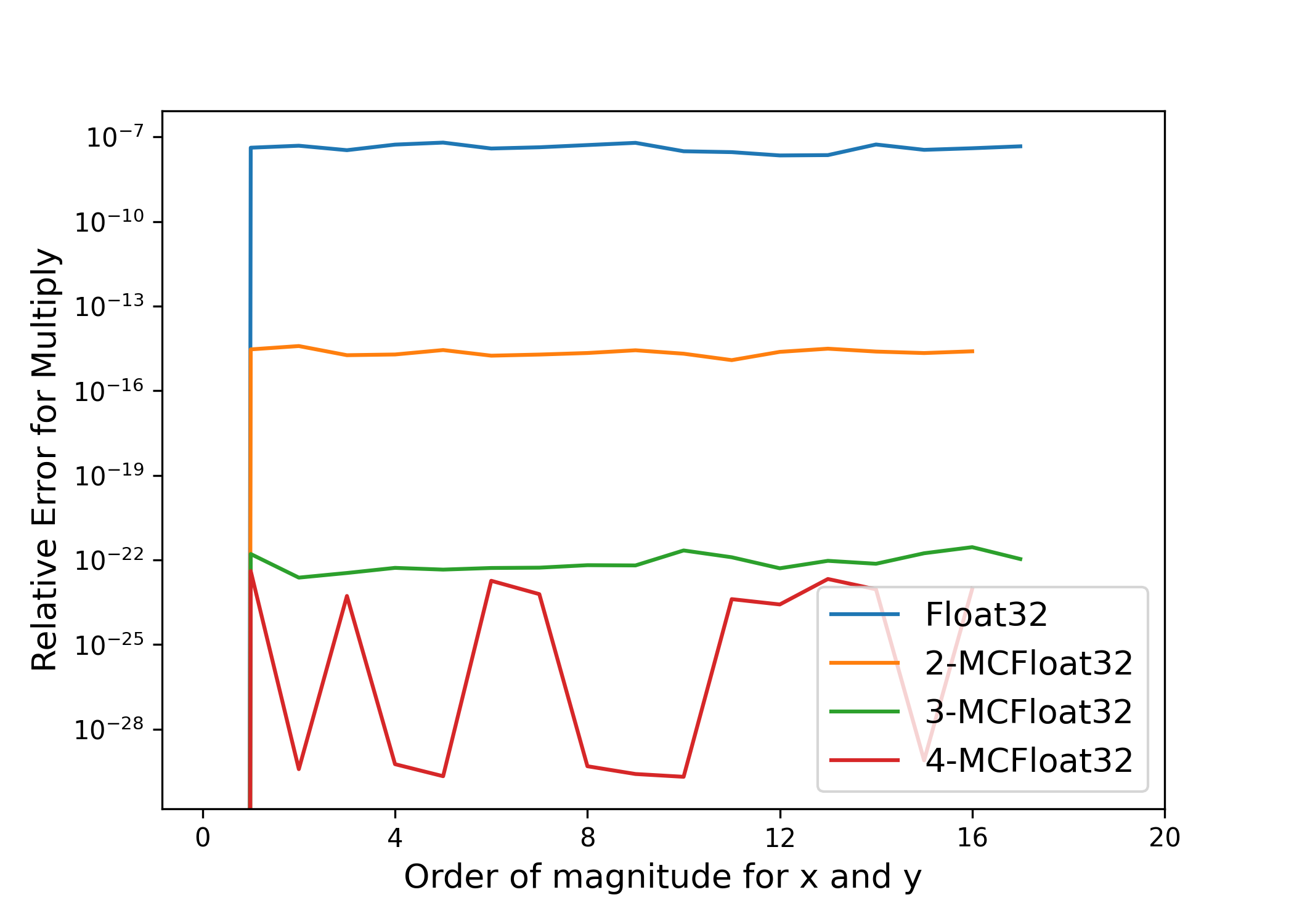
Figure 1: Relative Errors for Multiplication Mul-MCN(x,y), Compared with High Precision Julia BigFloat (3000 bits precision). Order of magnitudes for x and y are the same.

2.2 MCTensor Matrix Operators

After defining the basic MCF arithmetic, we are able to implement commonly used matrix level operators for MCTensor including AddMM-MCN (torch.addmm), Dot-MCN (torch.dot), MV-MCN (torch.mv), MM-MCN (torch.mm), BMM-MCN (torch.bmm) and Matmul-MCN (torch.matmul). Details of them are provided in the appendix.

For matrix operators, we leverage the broadcastability and vectorization from native PyTorch operations embedded in our basic MCF operators across each $nc$, and then apply sequential error propagation. For example, for MV-MCN with input as $x$ and $v$, we first use ScalingN to compute the broadcasted product of $x$ and $v$ for each $nc$, and then we sequentially sum up the results and propagate errors with the Add-MCN operator. In this way, we can make our multiplication part (ScalingN) independent of the input size and only employ for-loop for addition part (Add-MCN) since error propagation in the addition is sequential by the algorithm. Theoretically, accurate addition of $N$ MCTensors is of order at least $O(nc\cdot\log N)$.

MCTensor operators will be slower because of the need to propagate errors in computation, and have more memory burden than PyTorch operators because of the nature of MCF representation. In Table 1, we can see a tradeoff between program speed and precision. However, we would like to note that there is still much space to optimize these algorithms for better timing in practice. This work aims to provide ML community with the possibility to do high-precision computations for learning with MCTensor over GPUs. More details can be found in A.3.

⬇

class MCLinear(MCModule):

def __init__(self, in_features, out_features, nc, bias=True):

super(MCLinear, self).__init__()

self.in_features = in_features

self.out_features = out_features

self.nc = nc

self.weight = MCTensor(out_features, in_features, nc=nc, requires_grad=True)

if bias:

self.bias = MCTensor(out_features, nc=nc, requires_grad=True)

else:

self.bias = None

def forward(self, input):

return F.linear(input, self.weight, self.bias)

Figure 2: An Example for Implementing MCLinear

Operators	Inputs sizes	FloatTensor	1-MCTensor	2-MCTensor	3-MCTensor
Dot-MCN	$5000,5000$	$1.61\mu\text{s}\pm 3.29\text{ns}$	$442\mu\text{s}\pm 5.61\mu\text{s}$	$656\mu\text{s}\pm 1.16\mu\text{s}$	$858\mu\text{s}\pm 12.2\mu\text{s}$
MV-MCN	$(5000\times 500),500$	$157\mu\text{s}\pm 4.32\mu\text{s}$	$320\text{ms}\pm 5.78\text{ms}$	$460\text{ms}\pm 10.7\text{ms}$	$580\text{ms}\pm 12.1\text{ms}$
Matmul-MCN	( 500$\times$ 200), ( 200$\times$ 50)	$97.3\mu\text{s}\pm 1.1\mu\text{s}$	$495\text{ms}\pm 10.8\text{ms}$	$735\text{ms}\pm 21.7\text{ms}$	$934\text{ms}\pm 28\text{ms}$

Table 1: MCTensor Matrix Operators Running Time (mean $\pm$ sd)

2.3 MCModule, MCActivation, and MCOptim

We enable learning with MCTensor by developing neural network basic modules (MCModule), activation functions (MCActivation) and optimizers (MCOptim), in the exact programming interfaces as their PyTorch counterparts in (torch.nn.Module, torch.nn.functional and torch.optim). The semantics are identical to that of PyTorch’s module and optimizer, except that we are using MCTensor arithmetic. Specifically, we give some examples:

• MCModule: MCLinear, MCEmbedding, MCSequential

• MCOptim: MC-SGD, MCAdam

• MCActivation: MCSoftmax, MCReLU, MC-GELU

Here Fig.2 is the MCTensor implementation of linear layer, where weights and biases are represented by MCTensors. Similar to its PyTorch peer, a MCLinear takes input of size of input shape, in_features, size of output shape, out_features, learn with or without biases (boolean: bias) and number of component $nc$ for setting up the underlying MCTensors. To handle the operations within MCLinear layer, we override PyTorch’s nn.functional.linear to perform matrix level multiplication (Algo. 22) between a MCTensor weight and the Tensor input, then the addition of the product with bias (Algo.9) if needed. The output of the MCLinear layer is a MCTensor with the same $nc$.

Since we implemented MCModule, MCActivation, and MCOptimizer to follow the same specification as their PyTorch counterparts, building a MCTensor model is the same way as one would build a PyTorch module. The only difference to the users is the need to specify the number of components $nc$. An demonstration of our MCTensor model optimization programming paradigm can be found in Fig. 3.

⬇

mc_model = MCModel(nc=nc)

mc_optimizer = MCSGD(mc_model.parameters())

for x, y in train_dataset:

mc_optimizer.zero_grad()

y_hat = mc_model(x)

loss = loss_fn(y_hat, y)

loss.backward()

mc_optimizer.step()

Figure 3: MCTensor model optimization programming paradigm

2.4 Error Analysis

Principally, one can achieve arbitrary precision using MCTensor by simply increasing the number of components, however, note that each component of a MCTensor is a standard float, which has a natural range. Take Float16 for example, the minimum representable strictly positive value is $2^{-24}\approx 5.96\times 10^{-8}$, i.e., the smallest error that can be captured by MCFloat16 is $2^{-24}$. Hence in practice, 2-MCFloat16 is usually sufficient and similar performances are observed when more components of MCFloat16 were adopted. While simply adding an appropriate scale factor $2^{-k}$ (depending on the precision requirements) to smaller components can help capture even smaller errors, it is out of scope of this paper.

To validate improved precision of MCTensor models, we consider the linear regression task since it is possible to obtain loss arbitrarily close to zero. We use a single MCLinear without bias term and the Mean Squared Error (MSE) loss on fully observed synthetic data: $\mathcal{L}(W)=\text{MSELoss}(y,XW^{T})$, where $X$ is a $(10000\times 2)$ matrix with each entries sampled from $x\sim\mathcal{N}(-0.5,0.5^{2})$, and $y$ is calculated from $y=X{W^{*}}^{T}$ where $W^{*}$ is the $(10000\times 1)$ target weight sampled from $w^{*}\sim\mathcal{N}(-0.5,0.5^{2})$. We use gradient descent with $lr=0.05$ for optimization.

In Figure 4, we plot the training loss curves for the model with the same structure and initialization, but with MCTensor or Tensor as data structure. The comprehensive results can be seen in Table 6. The final train loss for 2-MCFloat16 is orders of magnitudes smaller than Float16.

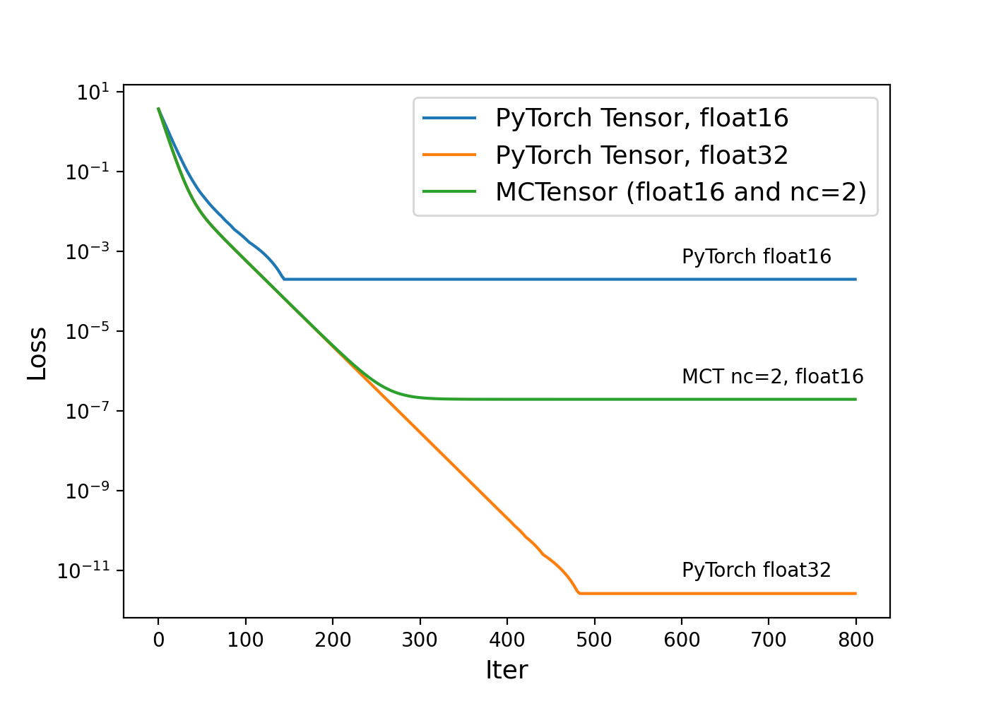
Figure 4: Loss Curves on Linear Regression Task.

Since by just using 2-MCFloat16, we can achieve much better precision than Float16 Tensor (HalfTensor), we run all following experiments in Float16 with $nc=$2 or 3 expect for Hyperbolic MCEmbedding.

3 Experiments

A MCTensor is able to achieve improved precision compared with a PyTorch Tensor with the same data type. If higher precision implies better results under the same experiment settings, we would expect our $n$-MCTensor ($n\geq 2$) model can achieve better performance than a native PyTorch model with same precision. We demonstrate the increasing precision under the same data type for MCTensor by carrying out experiments in two settings: (1) high precision learning with low precision numbers, this include logistic regression model and multi-layer perceptrons (MLP) in Section 3.1; and (2) high precision hyperbolic embedding reconstruction task in Section 3.2. For all these experiments, MCTensor models use the same initialization as the Tensor models, and use MCModule as its PyTorch’s nn.Module counterpart, with MCTensors as layer weights. Our code and models are open-source and available at github .

3.1 High-precision Computations with Low Precision

Low precision machine learning employs models that compute with low precision numbers (e.g. float8 and float16), which become popular in many edge-applications (Hubara et al., 2017; Zhang et al., 2019). However, the quantization error inherent with low precision arithmetic could affect the convergence and performance of the model (Wu et al., 2018; De Sa et al., 2018). As a matter of fact, most current low precision learning frameworks including (Courbariaux et al., 2014; De Sa et al., 2018) adopt high precision numbers during gradient computations and optimizations, but pursue a better way to convert the results to low-precision numbers with less quantization errors. In comparison, with MCTensor, one can get accurate update with purely low-precision numbers thoroughly without even touching high precision arithmetics. This is particularly helpful on devices where only low-precision arithmetics are supported.

Logistic Regression.

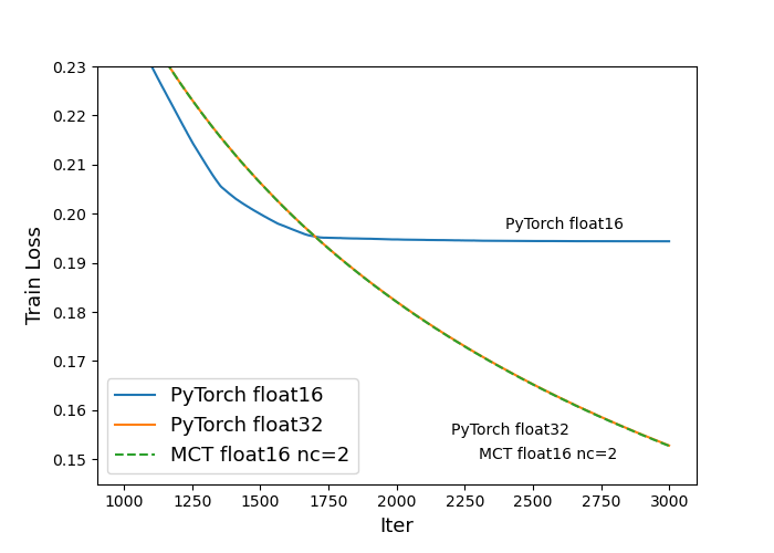
Figure 5: Training Losses for Logistic Regression Models on the Breast Cancer Dataset

We conduct a logistic regression task on a synthetic dataset and the cancer dataset, both are datasets with binary labels. The synthetic dataset consists of $1,000$ data points, where each data point contains two features. This dataset is constructed through the make_classification (Guyon, 2003) function from scikit-learn package with both n_informative and n_clusters_per_class are set to 1. The breast cancer dataset (MurtiRawat et al., 2020) consists of 569 data points and each data point contains 30 features. More details can be found in A.5.

Multi-layer Perceptron.

We also construct a Multi-layer Perceptron using MCTensor (MC-MLP) and evaluate it on classification tasks on the breast cancer dataset and a reduced MNIST, which has only 10,000 data points in total, with 1,000 images sampled randomly per class (Deng, 2012). The MC-MLP consists of three MCLinear layers with model weight in MCFloat16. After each MCLinear layer, the resulting MCTensor is transformed into a normal tensor, passed it to activation function and fed to the next layer.

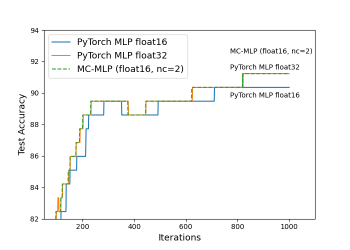
Figure 6: Test Accuracy for MC-MLP on Breast Cancer Dataset. Notice that the curve for MC-MLP model with nc=2, float16 essentially overlaps with the curve for PyTorch MLP model with float32.

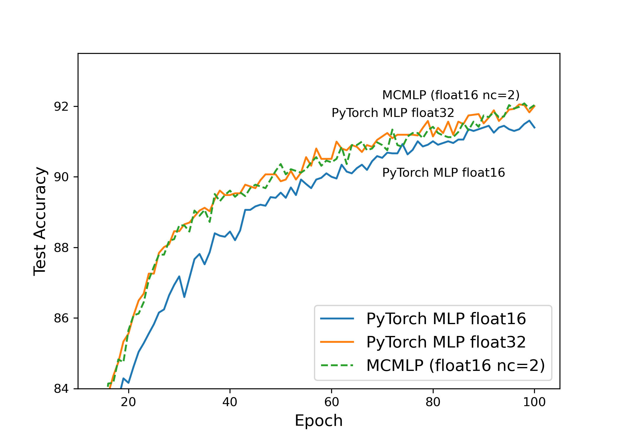
Figure 7: Test Accuracy for MC-MLP on Reduced MNIST Dataset. Notice that the curve for MC-MLP model with nc=2, float16 essentially overlaps with the curve for PyTorch MLP model with float32.

We experiment on both the Breast Cancer dataset and the Reduced MNIST dataset, and as demonstrated in Table 2 and Figure 7, in both experiments, MC-MLP outperforms PyTorch float16 models, and arrive at a lower training loss and a higher test accuracy (same as PyTorch float32 and float64 models). Notice that for both datasets, after $nc$ exceeds certain value ($nc=2$), adding extra more $nc$ would not lead to further improvement. More details can be found in Section A.7.

Model	Training Loss	Testing accuracy
MLP Float16	0.144	90.35
MLP Float32	0.124	91.23
MLP Float64	0.124	91.23
MC-MLP (nc=1)	0.144	90.35
MC-MLP (nc=2)	0.124	91.23
MC-MLP (nc=3)	0.124	91.23

Table 2: MC-MLP Models on Breast Cancer Dataset with MCSGD

3.2 Hyperbolic Embedding

Another use case that benefits from MCTensor is hyperbolic deep learning, where the non-Euclidean hyperbolic space is adopted in place of Euclidean space for various purposes. It has been shown in (Nickel & Kiela, 2017; Chami et al., 2019; Yu & De Sa, 2022) that hyperbolic space is better suited for processing hierarchical data (e.g. trees, acyclic graphs). However, representing hyperbolic space with ordinary floating-points (even float64) leads to unbounded representation error, particularly when points get far away from the origin, known as the “NaN" problem (Yu & De Sa, 2019) that not-a-number error occurs during computations. With MCTensor, we can achieve high-precision computations and avoid the “NaN" problem by simply using more components.

Following Yu & De Sa (2021), we conduct hyperbolic embedding experiment on the WordNet Mammals dataset with 1181 nodes and 6541 edges. We use Poincaré upper-half space (Halfspace) model to embed its transitive closure for reconstruction. The Poincaré Halfspace model is the manifold $(\mathcal{U}^{n},g_{u})$, where $\mathcal{U}^{n}$ is the upper half space of the $n$-dimensional Euclidean space, with the metric tensor and distance function being:

$$\textstyle g_{u}(\mathbf{x})=\frac{g^{E}}{x_{n}^{2}},~{}~{}~{}~{}d_{u}(\mathbf{x},\mathbf{y})=\text{arcosh}\left(1+\frac{||\mathbf{x}-\mathbf{y}||^{2}}{2x_{n}y_{n}}\right),$$

where $g^{E}$ is the Euclidean metric tensor. For the observed edges $\mathcal{D}=\{(\mathbf{x},\mathbf{y})\}$, we learn the embeddings $\Theta$ for all nodes, subject to minimizing the following loss function

$$\textstyle\mathcal{L}(\Theta)=\sum_{(\mathbf{x},\mathbf{y})\in D}\log\frac{e^{-d_{u}(\mathbf{x},\mathbf{y})}}{\sum_{\mathbf{y^{\prime}}\in\mathcal{N}(\mathbf{x})}e^{-d_{u}(\mathbf{x},\mathbf{y^{\prime}})}},$$

where $\mathcal{N}(\mathbf{x})$ are randomly chosen 50 negative examples in addition to the positive example $(\mathbf{x},\mathbf{y})$. We report the results in Table 3, where MAP is the mean averaged precision and MR is the mean rank metric.

Model	MAP (mean $\pm$ sd)	MR (mean $\pm$ sd)
Halfspace (f32)	$91.91\%\pm 0.64\%$	$1.399\pm 0.04$
Halfspace (f64)	$92.79\%\pm 0.41\%$	$1.340\pm 0.07$
MC-Halfspace (f64 nc=1)	$93.02\%\pm 0.40\%$	$1.296\pm 0.02$
MC-Halfspace (f64 nc=2)	$92.77\%\pm 0.28\%$	$1.304\pm 0.02$
MC-Halfspace (f64 nc=3)	$\textbf{93.31}\%\pm 0.75\%$	$\textbf{1.282}\pm 0.03$

Table 3: Performance of Hyperbolic Models

4 Conclusion

We introduce MCTensor based on PyTorch to achieve high-precision arithmetic while leveraging the benefits of heavily-optimized floating-point arithmetic. We verify its capability of high precision computations using low precision numbers and relieving the NaN problem in hyperbolic space. We hope this library could interest researchers to use MCTensor for ML applications requiring high-precision computations.

A promising future work is to design and optimize MCF algorithms to granularize the tradeoff between efficiency and precision to make MCTensor competent even for less-noisy and general tasks. We hope this library can address the need for fast high-precision library absent for DL community and prompt DL practitioners to rethink the concept of high-precision.

Appendix A Appendix

A.1 Julia BigFloat error

We further conduct experiments to evaluate the numerical errors of basic MCTensor arithmetic. Specifically, we first compute Add-MCN(x,y) of two random MCTensor x,y of roughly the same magnitude $m$. x,y are sampled by first sampling two random Julia BigFloat numbers with high precision (e.g. 3000 precision) using the equation $(10-\mathcal{N}(0,1))^{m}$, then converted to their corresponding MCTensors in Float32. In order to get the exact numerical error, we transform the MCTensor result to a Julia BigFloat number, then compute the relative error of it to the high precision addition of x,y (and not the addition of the two BigFloat numbers initially sampled) in Julia. In the same way, we compute the numerical errors of Mult-MCN(x,y) and ScalingN(x,y) with y being MCTensor in the former case and standard (PyTorch) tensor in the later case. x,y are sampled in the same way throughout the three cases.

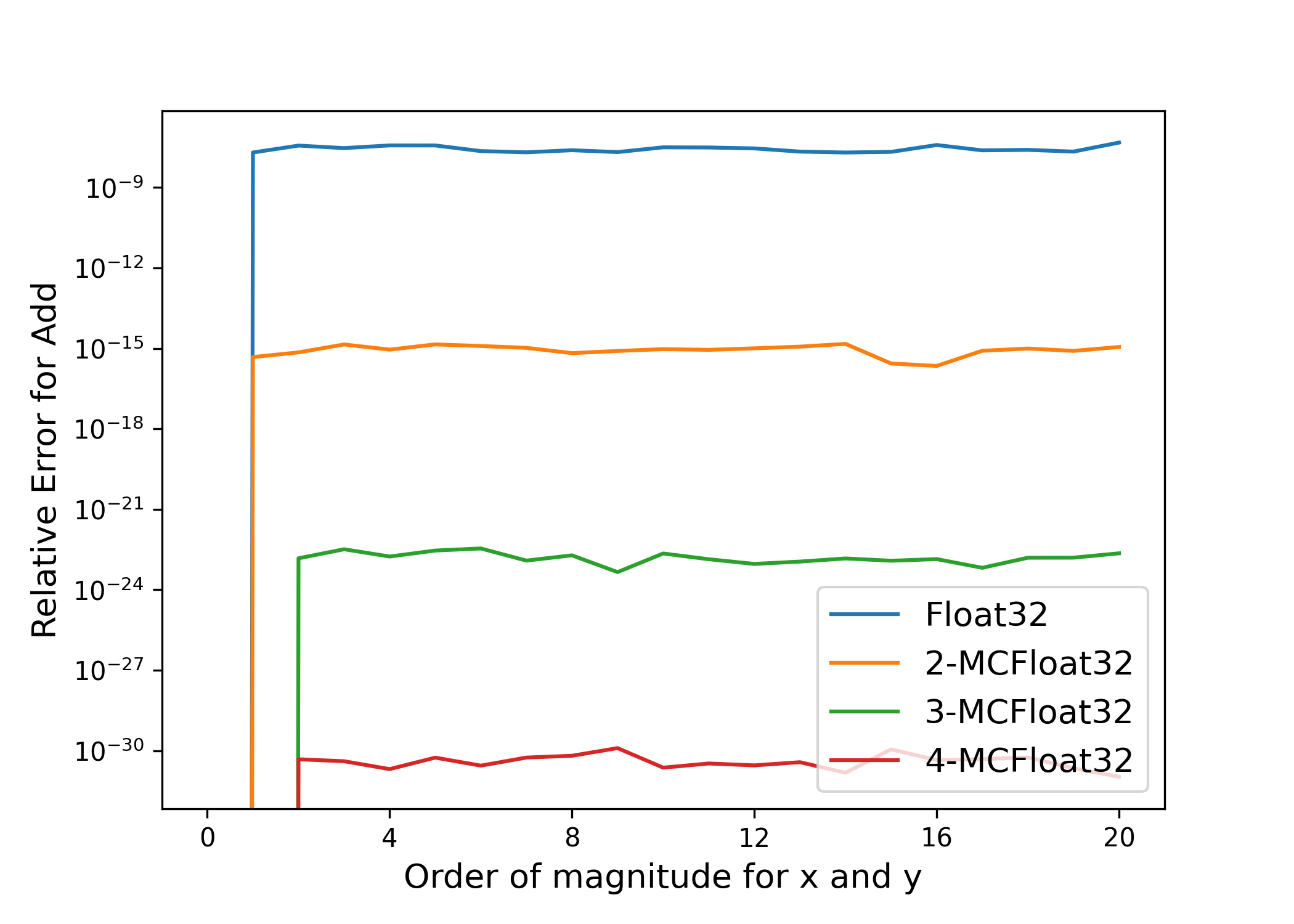
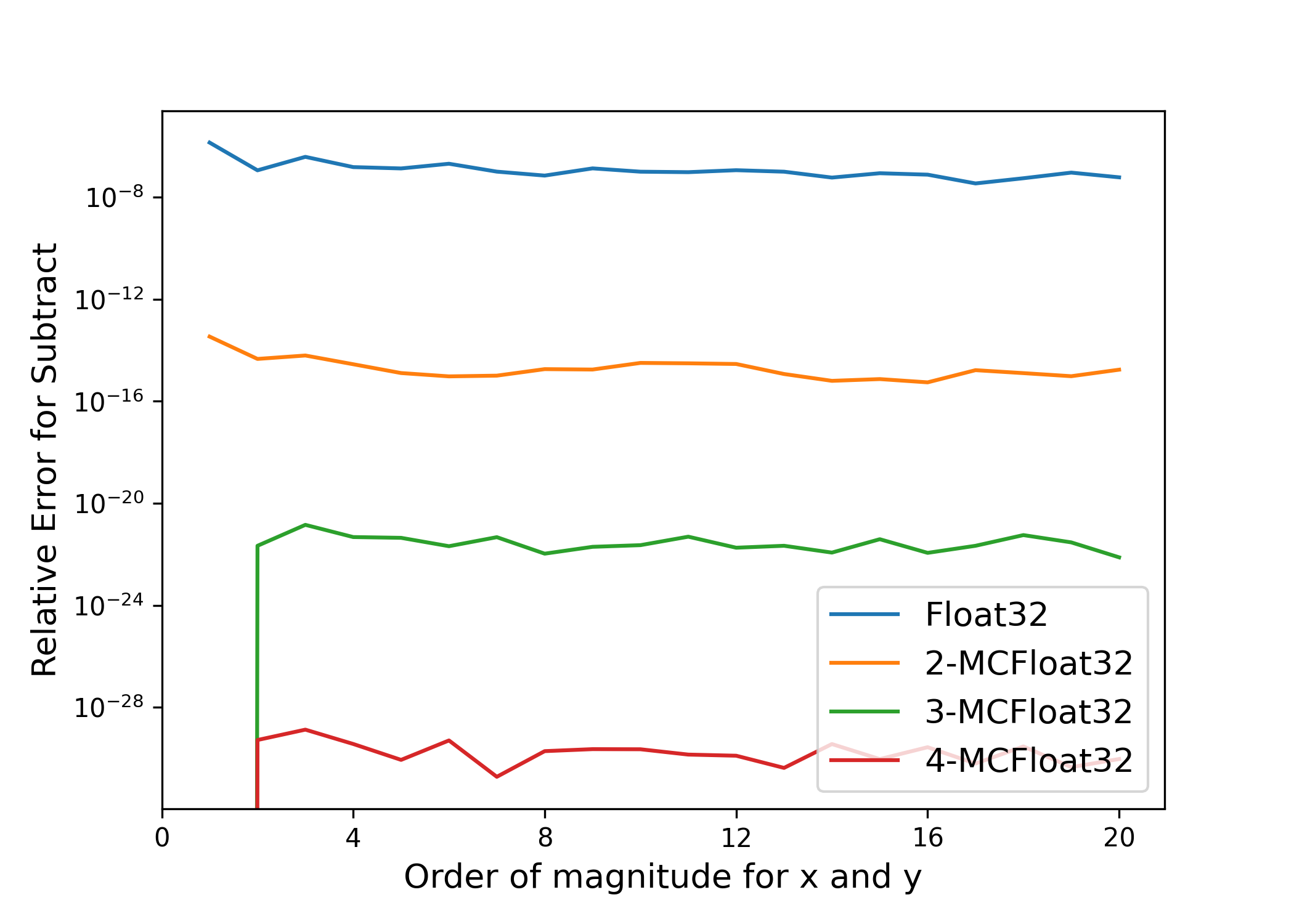
Figure 8: Relative Error of MCTensor arithmetic with different number of components, compared with high precision Julia BigFloat results (i.e. 3000 precision). Left: Add-MCN(x,y), middle: ScalingN(x,y) and right: Mult-MCN(x,y). Order of magnitudes for x and y are kept the same.

For a thorough comparison, we also derive below the same numerical errors when the order of magnitudes for x varies and order of magnitudes for y is kept at 2.

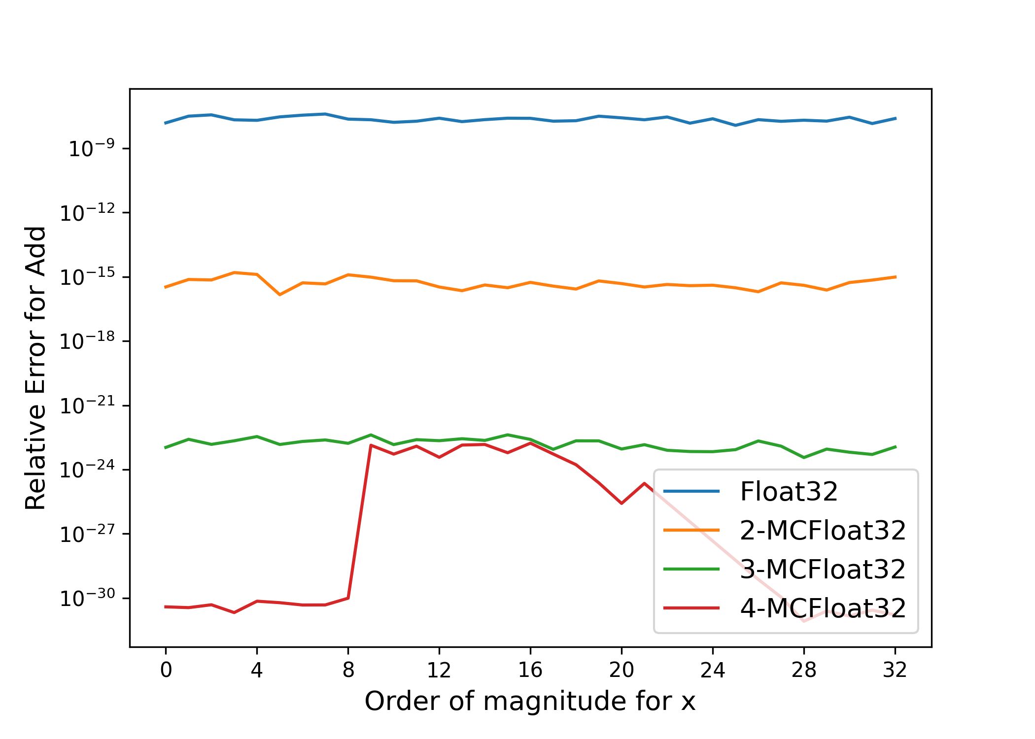
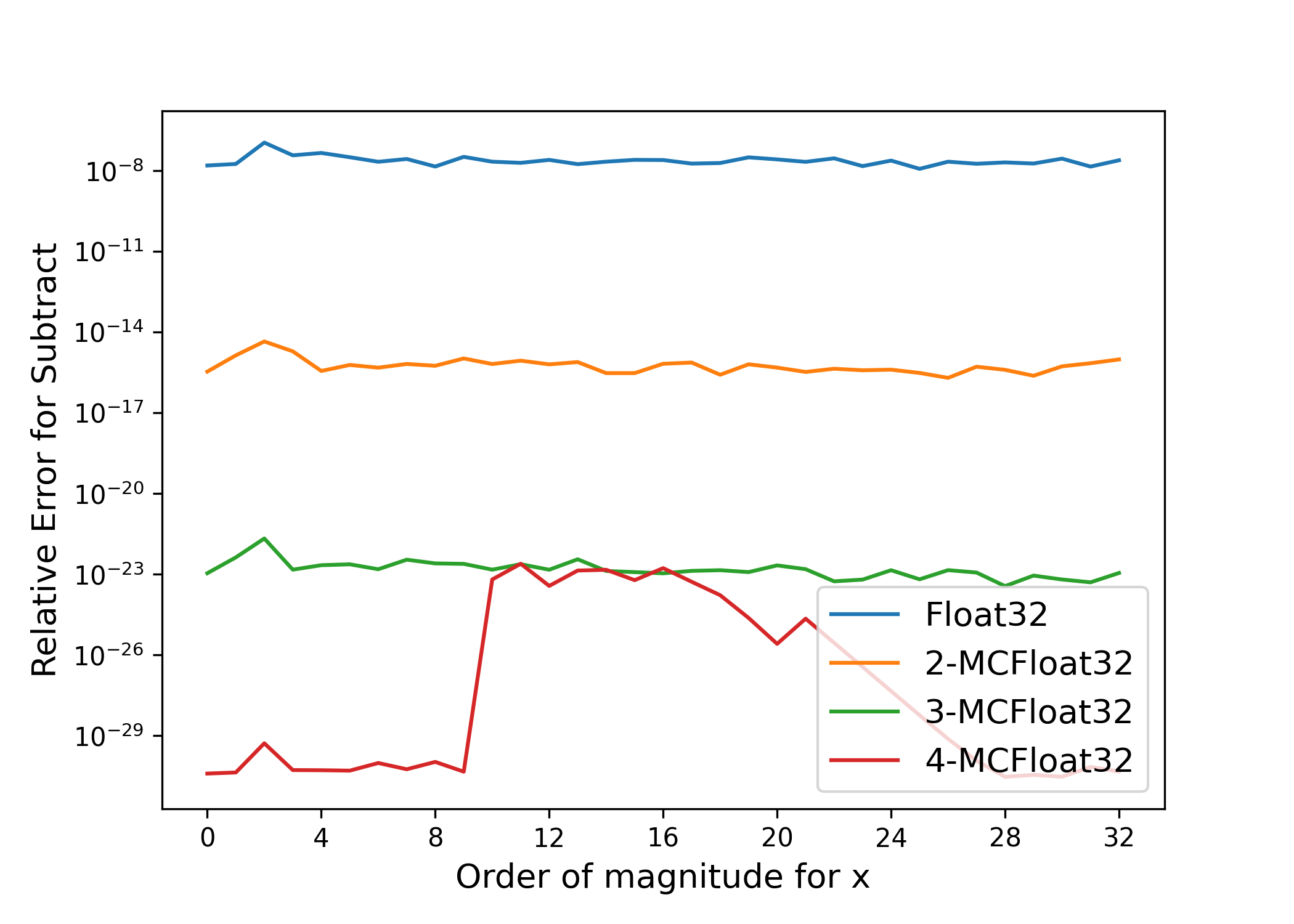
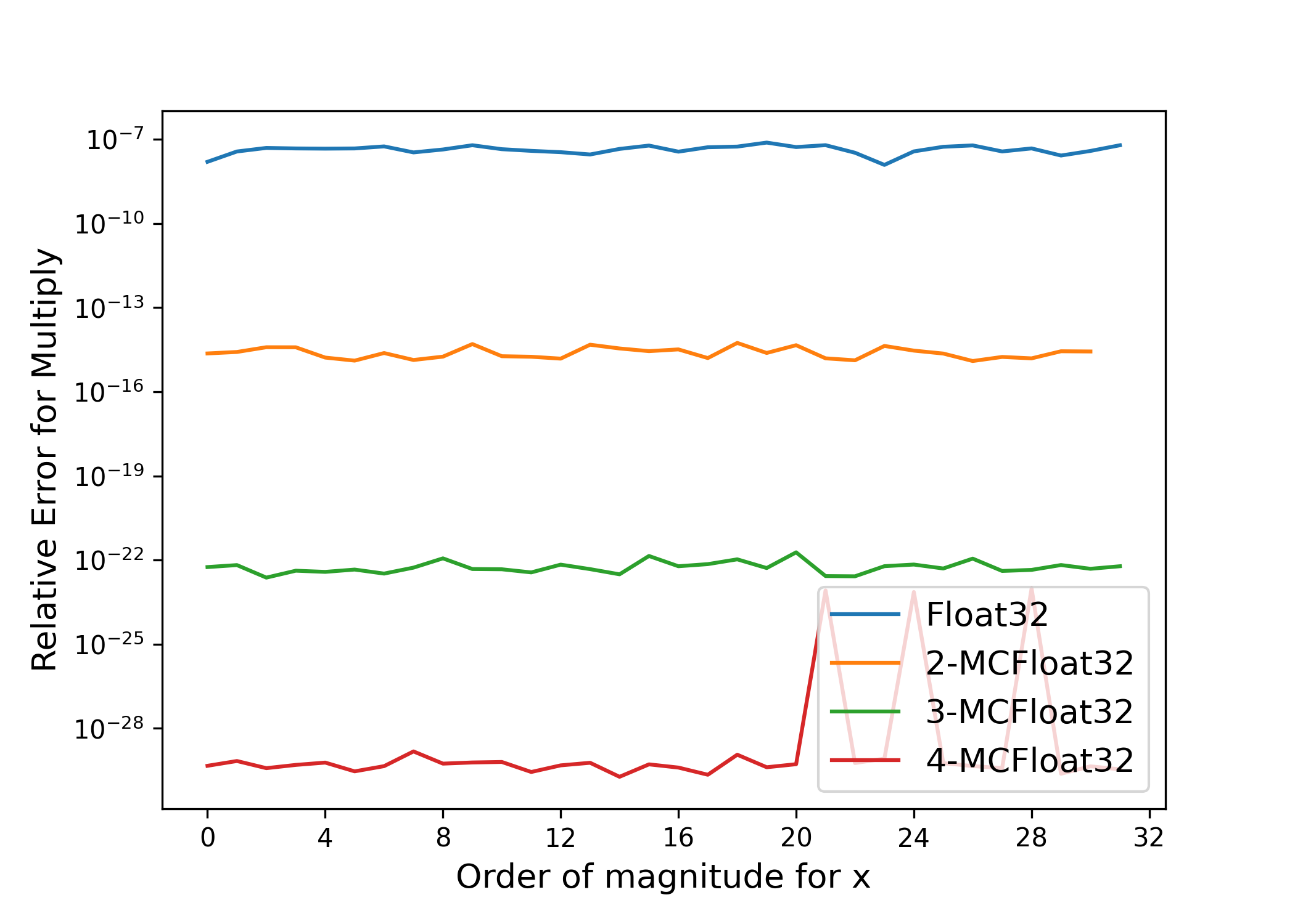
Figure 9: Relative Error of MCTensor arithmetic with different number of components, compared with high precision Julia BigFloat results (i.e. 3000 precision). Left: Add-MCN(x,y), middle: ScalingN(x,y) and right: Mult-MCN(x,y). Order of magnitudes for x varies and order of magnitudes for y is kept at 2.

A.2 MCTensor Operators

A.2.1 Basic Operators

The input of Two-Sum is two PyTorch Tensors with same precision, $a$ and $b$. Algorithm 2 returns the sum $s=\text{fl}(a+b)$ and the error, $err(a+b)$.

Algorithm 2 Two-Sum

  Input: PyTorch Tensors $a,b$

  $x\leftarrow a+b$

  $b_{\text{virtual}}\leftarrow\textbf{fl}(x-a)$

  $a_{\text{virtual}}\leftarrow\textbf{fl}(x-b_{\text{virtual}})$

  $b_{\text{roundoff}}\leftarrow\textbf{fl}(b-b_{\text{virtual}})$

  $a_{\text{roundoff}}\leftarrow\textbf{fl}(a-a_{\text{virtual}})$

  $y\leftarrow\textbf{fl}(a_{\text{roundoff}}+b_{\text{roundoff}})$

  Return: $(x,y)$

The Split Algorithm 3 takes a standard PyTorch floating point value with $p$-bit significand and splits it into its high and low parts, both with $\frac{p}{2}$-bit of significand.

Algorithm 3 Split

  Input: PyTorch Tensor $a$

  if $a.dtype$ is HalfTensor (float16) then

     $constant\leftarrow 6$

  else if $a.dtype$ is FloatTensor (float32) then

     $constant\leftarrow 12$

  else if $a.dtype$ is DoubleTensor (float64) then

     $constant\leftarrow 26$

  end if

  $t\leftarrow\textbf{fl}(2^{constant}+1)\cdot a$

  $a_{hi}\leftarrow\textbf{fl}(t-\textbf{fl}(t-a))$

  $a_{lo}\leftarrow\textbf{fl}(a-a_{hi})$

  Return: $(a_{hi},a_{lo})$

Based on Split, the following Algorithm 4 computes and returns $p=\textbf{fl}(a\times b)$ and $e=\text{err}(a\times b)$.

Algorithm 4 Two-Prod

  Input: PyTorch Tensors $a$, $b$

  $p\leftarrow\textbf{fl}(a\cdot b)$

  $(a_{hi},a_{lo})\leftarrow\textbf{Split}(a)$

  $(b_{hi},b_{lo})\leftarrow\textbf{Split}(b)$

  $err_{1}\leftarrow\textbf{fl}(p-\textbf{fl}(a_{hi}\cdot b_{hi}))$

  $err_{2}\leftarrow\textbf{fl}(err_{1}-\textbf{fl}(a_{lo}\cdot b_{hi}))$

  $err_{3}\leftarrow\textbf{fl}(err_{2}-\textbf{fl}(a_{hi}\cdot b_{lo}))$

  $e\leftarrow\textbf{fl}(\textbf{fl}(a_{lo}\cdot b_{lo})-err_{3})$

  Return: $(p,e)$

Fuse multiply-add, or FMA, is a floating-point operation that performs multiplication and addition in one step. With proper hardware, this Algorithm 5 can speed up TwoProd.

Algorithm 5 Two-Prod-fma

  Input: PyTorch Tensors $a$, $b$

  Requires: Machine supports FMA instructions set

  $p\leftarrow\textbf{fl}(a\cdot b)$

  $e\leftarrow$ torch.addcmul($-p,a,b$)

  Return: $(p,e)$

The constraint of decreasing magnitude and non-overlapping across $nc$ might be temporarily violated in computation, so MCTensor must be renormalized during computation. Users can specify the target $nc$ after renormalization, $r_{nc}$, but by default we keep them the same. The Renormalize function is this paper is a variant of the Priest’s algorithm 6. (Priest, 1991).

Algorithm 6 Renormalize (Priest, 1992)

  Input: $nc$-MCTensor $x$, $r_{nc}$

  Requires: $r_{nc}<nc$

  initialize $s\leftarrow x_{0},k\leftarrow 0,t_{0}\leftarrow 0$

  for $i=1$ to $nc$ do

     $(s,t_{i})\leftarrow\textbf{Two-Sum}(x_{i},s)$

  end for

  for $i=0$ to $nc-1$ do

     $(s,e)\leftarrow\textbf{Two-Sum}(s,t_{i})$

     if $e\neq 0$ then

        $b_{k}\leftarrow s$

        $s\leftarrow e$

        $k\leftarrow k+1$

     end if

  end for

  Return: $(b_{0},b_{1},\cdots,b_{r_{nc}-1})$

There is a simple and fast implementation of Renormalize as Simple-Renorm, which extracts all non-zero values from a non-renormalized MCTensor and puts together a new MCTensor. Note that this Simple-Renorm does not have the same guarantee as Renormalize. Therefore in our Mult-MCN, we still use the original version of Renormalize. But for most other operations, we still utilize Simple-Renorm for fast computation.

Algorithm 7 Simple-Renorm

  Input: $nc$-MCTensor $x$, $r_{nc}$

  Requires: $r_{nc}<nc$

  $k\leftarrow 0;\ (b_{0},b_{1},\cdots,b_{r_{nc}-1})\leftarrow(0,0,\cdots,0)$

  for $i=0$ to $r_{nc}-1$ do

     if $x_{i}\neq 0$ then

        $b_{k}\leftarrow x_{i}$

        ${k}\leftarrow k+1$

     end if

  end for

  Return: $(b_{0},b_{1},\cdots,b_{r_{nc}-1})$

Algorithm 8 describes the multiplication of a MCTensor with a PyTorch Tensor. In our implementation, the user can specify whether the algorithm can return an expanded results with $nc+1$, or a MCTensor with same $nc$.

Algorithm 8 ScalingN, modified from (Richard Shewchuk, 1997)

  Input: $nc$-MCTensor $x$, PyTorch Tensor $v$, $expand$

  initialize $e\leftarrow 0$

  for $i=0$ to $nc-1$ do

     $(h_{p},e_{1})\leftarrow\textbf{Two-Prod}(x_{i},v)$

     $(h_{i},e_{2})\leftarrow\textbf{Two-Sum}(h_{p},e)$

     $e\leftarrow\textbf{fl}(e_{1}+e_{2})$

  end for

  $h\leftarrow(h_{0},\cdots,h_{nc-1},e)$

  if $expand$ is True then

     Return: $\textbf{Simple-Renorm}(h,nc+1)$

  else

     Return: $\textbf{Simple-Renorm}(h,nc)$

  end if

Add-MCN, Div-MCN, Mult-MCN are operators for addition, division, and multiplication of two $nc$-MCTensors. Here we have two versions of multiplication, Mult-MCN and Mult-MCN-Slow. Algorithm 11 is implemented by taking the inverse of the second MCTensor first, and then the first MCTensor is divided by the second MCTensor’s inverse. This division would give the result of multiplication. Algorithm 12 follows the same pattern of our definition of Div-MCN and provides better error bounds, but it is rarely used as the computational cost is too high.

Algorithm 9 Add-MCN, modified from (Richard Shewchuk, 1997)

  Input: $nc$-MCTensor $x,y$

  initialize: $e\leftarrow 0$

  for $i=0$ to $nc-1$ do

     $(h_{p},e_{1})\leftarrow\textbf{Two-Sum}(x_{i},y_{i})$

     $(h_{i},e_{2})\leftarrow\textbf{Two-Sum}(h_{p},e)$

     $e\leftarrow\textbf{fl}(e_{1}+e_{2})$

  end for

  $h\leftarrow(h_{0},\cdots,h_{nc-1},e)$

  Return: Simple-Renorm$(h,nc)$

Algorithm 10 Div-MCN, modified from (Richard Shewchuk, 1997)

  Input: $nc$-MCTensor $x,y$

  initialize: $q\leftarrow\textbf{fl}(x_{0}/y_{0}),h_{0}\leftarrow q$

  for $i=1$ to $nc$ do

     $r\leftarrow\textbf{Add-MCN}(x,-\textbf{ScalingN}(y,q,\text{False}))$

     $x\leftarrow r$

     $q\leftarrow\textbf{fl}(x_{0}/y_{0})$

     $h_{i}\leftarrow q$

  end for

  $h\leftarrow(h_{0},h_{1},\cdots,h_{nc})$

  Return: Simple-Renorm$(h,nc)$

Algorithm 11 Mult-MCN

  Input: $nc$-MCTensor $x,y$

  initialize: $z_{0}\leftarrow 1,z_{1}=\cdots=z_{nc-1}\leftarrow 0$

  $z\leftarrow(z_{0},z_{1},\cdots,z_{nc-1})$

  $y^{-1}\leftarrow\textbf{Renormalize}(\textbf{Div-MCN}(z,y))$

  $h\leftarrow\textbf{Renormalize}(\textbf{Div-MCN}(x,y^{-1}))$

  Return: $h$

Algorithm 12 Mult-MCN-Slow

  Input: $nc$-MCTensor $x,y$

  initialize: $p\leftarrow\textbf{fl}(x_{0}\cdot y_{0}),h_{0}\leftarrow p$

  for $i=1$ to $nc$ do

     $e\leftarrow\textbf{Add-MCN}(x,-\textbf{DivN}(p,y))$

     $x\leftarrow e$

     $p\leftarrow\textbf{fl}(x_{0}\cdot y_{0})$

     $h_{i}\leftarrow p$

  end for

  $h\leftarrow(h_{0},h_{1},\cdots,h_{nc})$

  Return: Simple-Renorm$(h,nc)$

Algorithm 13, DivN takes input of a PyTorch Tensor and a MCTensor and computes the Div-MCN results by appending zero-value components to a PyTorch Tensor and making it MCTensor.

Algorithm 13 DivN

  Input: PyTorch Tensor $x_{0}$, $nc$-MCTensor $y$,

  initialize: $x_{1}=\cdots=x_{nc-1}\leftarrow 0$

  $x\leftarrow(x_{0},x_{1},\cdots,x_{nc-1})$

  Return: Div-MCN$(x,y)$

The following Algorithm 14 describes the exponential function for a MCTensor.

Algorithm 14 Exp-MCN

  Input: $nc$-MCTensor $x$

  initialize $h\leftarrow\text{exp}(x_{0})$

  for $i=1$ to $nc-1$ do

     $h\leftarrow\textbf{ScalingN}(h,\text{exp}(h_{i}),\text{True})$

  end for

  Return: $h$

The following Algorithm 15 describes the square of a MCTensor.

Algorithm 15 Square-MCN

  Input: $nc$-MCTensor $x$

  initialize $h_{0}\leftarrow\textbf{fl}(2^{x_{0}}),h_{1}=\cdots=h_{nc-1}\leftarrow 0$

  $h\leftarrow(h_{0},h_{1},\cdots,h_{nc-1})$

  $h\leftarrow\textbf{Grow-ExpN}(h,\textbf{fl}(2\cdot x_{0}\cdot x_{1}))$

  Return: $h$

A.2.2 Matrix Operators

Based on the dimensions of input MCTensor and PyTorch Tensor, Dot-MCN, MV-MCN, MM-MCN, BMM-MCN and 4DMM-MCN are implemented for calculating the matrix-level multiplication results. All operations are identical with the PyTorch implementations.

Algorithm 16 Dot-MCN

  Input: $nc$-MCTensor $x$, PyTorch Tensor $v$

  Requires: $x$ and $v$ both 1D array

  $h\leftarrow\textbf{ScalingN}(x,v,\text{False})$

  $h_{tensor}=h_{0}+h_{1}+\cdots+h_{nc-1}$

  Return: $h_{tensor}$

Algorithm 17 MV-MCN

  Input: $nc$-MCTensor $x$, PyTorch Tensor $v$

  Requires: $x$ is 2D matrix of size $(n\times m)$ and $v$ is 1D array of size $m$

  $scaled\leftarrow\textbf{ScalingN}(x,v,\text{False})$

  $h\leftarrow scaled[...,0]$

  for $i=1$ to $m-1$ do

     $h\leftarrow\textbf{Add-MCN}(h,scaled[...,i])$

  end for

  Return: $h$

Algorithm 18 MM-MCN

  Input: $nc$-MCTensor $x$, PyTorch Tensor $v$

  Requires: $x$ is 2D matrix of size $(n\times m)$ and $v$ is 2D Matrix of size $(m\times p)$

  $x\leftarrow x.\textbf{unsqueeze}(-1)$

  $v\leftarrow v.\textbf{transpose}(-1,-2)$

  $scaled\leftarrow\textbf{ScalingN}(x,v,\text{False})$

  $h\leftarrow scaled[...,0]$

  for $i=1$ to $m-1$ do

     $h\leftarrow\textbf{Add-MCN}(h,scaled[...,i])$

  end for

  Return: $h$

Algorithm 19 BMM-MCN

  Input: $nc$-MCTensor $x$, PyTorch Tensor $v$

  Requires: $x$ is 3D matrix of size $(b\times n\times m)$ and $v$ is 3D Matrix of size $(b\times m\times p)$

  $x\leftarrow x.\textbf{unsqueeze}(-1)$

  $v\leftarrow v.\textbf{unsqueeze}(1).\textbf{transpose}(-1,-2)$

  $scaled\leftarrow\textbf{ScalingN}(x,v,\text{False})$

  $h\leftarrow scaled[...,0]$

  for $i=1$ to $m-1$ do

     $h\leftarrow\textbf{Add-MCN}(h,scaled[...,i])$

  end for

  Return: $h$

Algorithm 20 4DMM-MCN

  Input: $nc$-MCTensor $x$, PyTorch Tensor $v$

  Requires: $x$ is 4D matrix of size $(a\times b\times n\times m)$ and $v$ is 4D Matrix of size $(c\times d\times m\times p)$; two sizes can be broadcasted in torch.matmul

  $x\leftarrow x.\textbf{unsqueeze}(-1)$

  $v\leftarrow v.\textbf{unsqueeze}(2).\textbf{transpose}(-1,-2)$

  $scaled\leftarrow\textbf{ScalingN}(x,v,\text{False})$

  $h\leftarrow scaled[...,0]$

  for $i=1$ to $m-1$ do

     $h\leftarrow\textbf{Add-MCN}(h,scaled[...,i])$

  end for

  Return: $h$

The following Algorithm 21 computes the matrix multiplication of a $nc$-MCTensor with a PyTorch Tensor first, then times a constant $\alpha$. Then the product of another $nc$-MCTensor times a constant $\beta$ is added to the former multiplication result.

Algorithm 21 AddMM-MCN

  Input: $nc$-MCTensor $x$, $nc$-MCTensor $y$, PyTorch Tensor $v$, $\beta$, $\alpha$

  Requires: $x$ is 2D matrix of size $(n\times m)$, and $v$ is 2D Matrix of size $(m\times p)$; $y$ is 2D matrix of size $(n\times m)$ or $y$ is 1D array of size $m$

  $h\leftarrow\textbf{ScalingN}(\textbf{MM-MCN}(x,v),\alpha)$

  $bias\leftarrow\textbf{ScalingN}(y,\beta)$

  $h\leftarrow\textbf{Add-MCN}(h,bias)$

  Return: $h$

This Algorithm 22, Matmul-MCN is the central function for handling all matrix level multiplications of one $nc$-MCTensor and one PyTorch Tensor.

Algorithm 22 Matmul-MCN

  Input: $nc$-MCTensor $x$, PyTorch Tensor $y$

  $x_{d},y_{d}\leftarrow x.\textbf{dim()},y.\textbf{dim()}$

  if $x_{d}=1$ and $y_{d}=1$ then

     Return: $\textbf{Dot-MCN}(x,y)$

  else if $x_{d}=2$ and $y_{d}=2$ then

     Return: $\textbf{MM-MCN}(x,y)$

  else if $x_{d}=2$ and $y_{d}=1$ then

     Return: $\textbf{MV-MCN}(x,y)$

  else if $x_{d}>2$ and $y_{d}=1$ then

     Return: $\textbf{ScalingN}(x,y)$

  else if $x_{d}=y_{d}$ and $x_{d}=3$ then

     Return: $\textbf{BMM-MCN}(x,y)$

  else if $x_{d}=y_{d}$ and $x_{d}=4$ then

     Return: $\textbf{4DMM-MCN}(x,y)$

  end if

A.3 MCF Basic and Matrix Operators

We run on a AMD Ryzen 7 5800X CPU with 64 GB memory.

For all the basic operators, we repeat PyTorch addition for 7e3 runs and 1-, 2-, 3-MCTensor for 7 runs.

For vector-vector (torch.dot/Dot-MCN) product, we repeat PyTorch addition for 7e6 runs and 1-, 2-, 3-MCTensor for 7e3 runs. For matrix-vector (torch.mv/MV-MCN) product and batched matrix-matrix (torch.bmm/BMM-MCN) product, we repeat PyTorch addition for 7e3 runs and 1-, 2-, 3-MCTensor for 7 runs. For matrix-matrix (torch.matmul/Matmul-MCN) product and bias-matrix-matrix (torch.addmm/AddMM-MCN) addition-product, we repeat PyTorch addition for 7e4 runs and 1-, 2-, 3-MCTensor for 7 runs.

The timing for both matrix and basic operators are given in Table 4 and Table 5.

Operators	Inputs sizes	FloatTensor	1-MCTensor	2-MCTensor	3-MCTensor
Add-MCN	$(1000\times 1000)$	$497\ \mu\text{s}\pm 6.77\ \mu\text{s}$	$26.7\ \text{ms}\pm 486\ \mu\text{s}$	$44.7\ \text{ms}\pm 379\ \mu\text{s}$	$64.4\ \text{ms}\pm 385\ \mu\text{s}$
ScalingN	$(1000\times 1000)$	$490\ \mu\text{s}\pm 9.69\ \mu\text{s}$	$33.7\ \text{ms}\pm 402\ \mu\text{s}$	$57.5\ \text{ms}\pm 842\ \mu\text{s}$	$84.7\ \text{ms}\pm 1.78\ \text{ms}$
Mult-MCN	$(1000\times 1000)$	$514\ \mu\text{s}\pm 15.2\ \mu\text{s}$	$218\ \text{ms}\pm 4.03\ \text{ms}$	$667\ \text{ms}\pm 11.6\ \text{ms}$	$1.4\ s\pm 21.6\ \text{ms}$
Div-MCN	$(1000\times 1000)$	$510\ \mu\text{s}\pm 10.6\ \mu\text{s}$	$80.3\ \text{ms}\pm 770\ \mu\text{s}$	$243\ \text{ms}\pm 3.24\ \text{ms}$	$498\ \text{ms}\pm 8.26\ \text{ms}$

Table 4: MCTensor Basic Operators Running Time (mean $\pm$ sd)

Operators	Inputs sizes	FloatTensor	1-MCTensor	2-MCTensor	3-MCTensor
Dot-MCN	$5000,5000$	$1.61\ \mu\text{s}\pm 3.29\ \text{ns}$	$442\ \mu\text{s}\pm 5.61\ \mu\text{s}$	$656\ \mu\text{s}\pm 1.16\ \mu\text{s}$	$858\ \mu\text{s}\pm 12.2\ \mu\text{s}$
MV-MCN	$(5000\times 500),500$	$157\ \mu\text{s}\pm 4.32\mu\text{s}$	$320\ \text{ms}\pm 5.78\text{ms}$	$460\ \text{ms}\pm 10.7\text{ms}$	$580\ \text{ms}\pm 12.1\text{ms}$
Matmul-MCN	( 500$\times$ 200), ( 200$\times$ 50)	$97.3\ \mu\text{s}\pm 1.1\ \mu\text{s}$	$495\ \text{ms}\pm 10.8\ \text{ms}$	$735\ \text{ms}\pm 21.7\ \text{ms}$	$934\ \text{ms}\pm 28\ \text{ms}$
AddMM-MCN	100, ( 500$\times$ 200), ( 200$\times$ 100),	$153\ \mu\text{s}\pm 869\ \text{ns}$	$750\ \text{ms}\pm 21.9\ \text{ms}$	$1.12\ \text{s}\pm 28.4\ \text{ms}$	$1.44\ \text{s}\pm 49.1\ \text{ms}$
BMM-MCN	(16 $\times$ 500$\times$ 200), (16 $\times$200$\times$ 50)	$1.5\ \text{ms}\pm 9.32\ \mu\text{s}$	$4.84\ \text{s}\pm 43.1\ \text{ms}$	$8.03\ \text{s}\pm 68.4\ \text{ms}$	$11.2\ \text{s}\pm 74.1\ \text{ms}$

Table 5: MCTensor Matrix Operators Running Time (mean $\pm$ sd)

A.4 Linear Regression Results

Table 6 describes the final training loss of the linear regression task in section 2.4.

Model	Train Loss
PyTorch float16	1.99e-4
PyTorch float32	2.64e-12
PyTorch float64	8.02e-18
MCTensor float16, nc = 1	1.80e-4
MCTensor float32, nc = 2	1.95e-7
MCTensor float64, nc = 3	1.95e-7

Table 6: Final Training Loss Results of Linear Regression Task

A.5 Logistic Regression

We apply logistic regression on a synthetic dataset and a breast cancer dataset. The synthetic dataset consists of 1,000 data points, where each data point contains two features, while the breast cancer dataset consists of 569 data points and each data point contains 30 numeric features. A single MCLinear layer with float16 and $nc$ between 1, 2 and 3 are used for logistic regression with Binary Cross Entropy loss.

$${\mathcal{L}(W)={\leavevmode\lstinline{{\lst@@@set@language\lst@@@set@numbers\lst@@@set@frame\lst@@@set@rulecolor\lst@@@set@language\lst@@@set@frame\color[rgb]{0.35,0.22,0.21}{\@listingGroup{ltx_lst_identifier}{BCELoss}}}}}}(y,\text{sigmoid}(XW^{T}))$$

For both datasets, we randomly split 80% of the data for training and 20% of the data for testing. As both datasets are small in scale, we run them in full batch with MC-SGD and SGD. For the synthetic dataset, we set learning rate to be 3e-3 and run for 4000 epochs. For the breast cancer dataset, we set learning rate to be 1e-4 and momentum as 0.9, and run for 3000 epochs. Below is the results for both dataset and figures for MCLinear results on breast cancer dataset with MC-SGD optimizer. As can be seen, even with as few as 2 components, MCTensor in float16 can match with the training loss of float32 Tensor.

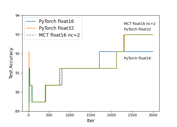
Figure 10: Testing Accuracy for MCTensor and PyTorch Logistic Regression on the Breast Cancer Dataset

Model	Training Loss	Testing Accuracy (%)
Tensor float16	0.1940	100
Tensor float32	0.1042	100
Tensor float64	0.1042	100
1-MCTensor float16	0.1941	100
2-MCTensor float16	0.1041	100
3-MCTensor float16	0.1041	100

Table 7: Final Training and Testing Results for Logistic Regression on Synthetic Dataset

Model	Training Loss	Testing Accuracy (%)
Tensor float16	0.1944	92.11
Tensor float32	0.1528	92.98
Tensor float64	0.1528	92.98
1-MCTensor float16	0.1944	92.11
2-MCTensor float16	0.1527	92.98
3-MCTensor float16	0.1527	92.98

Table 8: Final Training and Testing Results for Logistic Regression on Breast Cancer Dataset

A.6 MCTensor Deep Learning models

As a demonstration for the ease of using MCTensor to build a MCTensor deep learning model, we provide an example code for MCTensor MLP (MC-MLP) model for the multi-class classification tasks. Essentially, the only differences visible to the users are the need to set the number of components, and the need to convert MCTensor output to Tensor approximation between different layers. The need for Tensor approximation is explained below.

⬇

class MC-MLP(MCModule):

def __init__(self, input_dim, hidden1, hidden2, num_classes=10, nc=2):

super(MCMLP, self).__init__()

self.fc1 = MCLinear(input_dim, hidden1, nc=nc)

self.fc2 = MCLinear(hidden1, hidden2, nc=nc)

self.fc3 = MCLinear(hidden2, num_classes, nc=nc)

self.dropout = nn.Dropout(0.2)

def forward(self, x):

x = F.relu(self.fc1(x))

x = self.dropout(x.tensor.sum(-1))

x = F.relu(self.fc2(x))

x = self.dropout(x.tensor.sum(-1))

x = self.fc3(x)

return F.log_softmax(x.tensor.sum(-1), dim=1)

Figure 11: MC-MLP Code Example

In MCModule, all network layers take Tensor as inputs, keep MCTensor as their weights, and through MCTensor matrix operations, produces MCTensor as output. If the MCTensor outputs need to be taken as input for the next MCModule layer, there need to be new layers that will perform multiplication on two MCTensor matrices. As can be seen from Table 4, ScalingN, the multiplication between a MCTensor and a PyTorch Tensor, is more than a hundred times faster than Mult-MCN, the multiplication between two MCTensor. To avoid this forbidden cost of computation, we convert the unevaluated sums into an evaluated sum as shown above (x.tensor.sum(-1)). Although there might some losses of precision due to summation, the loss is marginal and we trade it for an orders of magnitude smaller execution time.

A.7 MC-MLP Experiment Details

Using MC-MLP, we perform multi-class classification task on the Reduced MNIST dataset and binary classification task on the Breast Cancer dataset. The training details for both tasks are shown in Table 9 and Table 10.

Parameter	Value
MLP first hidden layer dim	150
MLP second hidden layer dim	150
Batch size	full batch (569)
Optimizer	MC-SGD (GD with full batch)
Learning rate	6e-3
Epoch	1000

Table 9: Training Details for the Breast Cancer dataset

Parameter	Value
MLP first hidden layer dim	50
MLP second hidden layer dim	50
Batch size	128
Optimizer	MC-SGD (SGD)
Learning rate	2e-3
Momentum	0.8
Epoch	100

Table 10: Training Details for the Reduced MNIST Dataset

Figure 12 shows the training loss curves for MC-MLP on breast cancer dataset with MC-SGD optimizer.

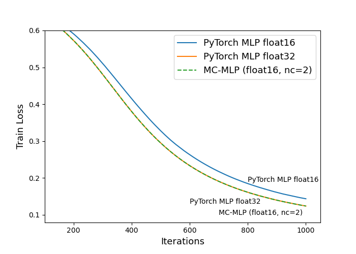
Figure 12: Training Loss Curves for MLP on Breast Cancer Dataset

Figure 13 shows the training loss curves for MC-MLP on reduced MNIST dataset with MC-SGD optimizer. The hyperparameters used in training are shown in Table 10, and the final results for testing accuracy is shown in Table 11.

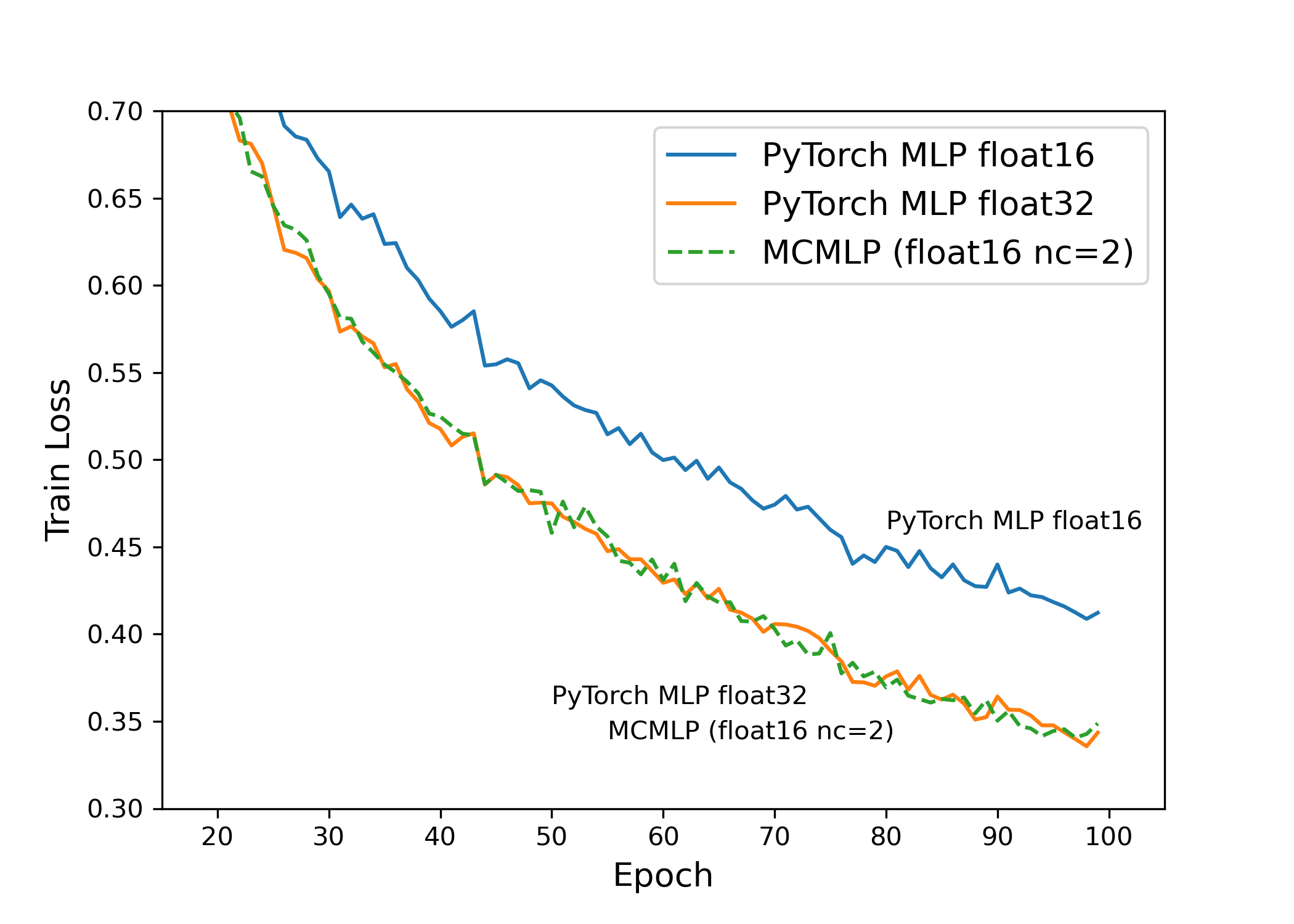
Figure 13: Training Loss Curves for MLP on Reduced MNIST Dataset

Model	Training Loss	Testing accuracy
MCMLP (f16 nc=1)	0.424	91.40
MCMLP (f16 nc=2)	0.349	92.03
MCMLP (f16 nc=3)	0.349	91.98
PyTorch MLP (f16)	0.412	91.40
PyTorch MLP (f32)	0.343	92.00
PyTorch MLP (f64)	0.343	92.00

Table 11: MC-MLP Models on Reduced MNIST Dataset with MCSGD

References

- Abadi et al. (2015) Abadi, M., Agarwal, A., Barham, P., Brevdo, E., Chen, Z., Citro, C., Corrado, G. S., Davis, A., Dean, J., Devin, M., Ghemawat, S., Goodfellow, I., Harp, A., Irving, G., Isard, M., Jia, Y., Jozefowicz, R., Kaiser, L., Kudlur, M., Levenberg, J., Mané, D., Monga, R., Moore, S., Murray, D., Olah, C., Schuster, M., Shlens, J., Steiner, B., Sutskever, I., Talwar, K., Tucker, P., Vanhoucke, V., Vasudevan, V., Viégas, F., Vinyals, O., Warden, P., Wattenberg, M., Wicke, M., Yu, Y., and Zheng, X. TensorFlow: Large-scale machine learning on heterogeneous systems, 2015. URL https://www.tensorflow.org/. Software available from tensorflow.org.
- Bailey & Borwein (2015) Bailey, D. H. and Borwein, J. M. High-precision arithmetic in mathematical physics. Mathematics, 3(2):337–367, 2015.
- Bezanson et al. (2017) Bezanson, J., Edelman, A., Karpinski, S., and Shah, V. B. Julia: A fresh approach to numerical computing. SIAM review, 59(1):65–98, 2017.
- Chami et al. (2019) Chami, I., Ying, Z., Ré, C., and Leskovec, J. Hyperbolic graph convolutional neural networks. Advances in neural information processing systems, 32, 2019.
- Chen et al. (2015) Chen, T., Li, M., Li, Y., Lin, M., Wang, N., Wang, M., Xiao, T., Xu, B., Zhang, C., and Zhang, Z. Mxnet: A flexible and efficient machine learning library for heterogeneous distributed systems. arXiv preprint arXiv:1512.01274, 2015.
- Courbariaux et al. (2014) Courbariaux, M., Bengio, Y., and David, J.-P. Training deep neural networks with low precision multiplications. arXiv preprint arXiv:1412.7024, 2014.
- De Sa et al. (2018) De Sa, C., Leszczynski, M., Zhang, J., Marzoev, A., Aberger, C. R., Olukotun, K., and Ré, C. High-accuracy low-precision training. arXiv preprint arXiv:1803.03383, 2018.
- Deng (2012) Deng, L. The mnist database of handwritten digit images for machine learning research [best of the web]. IEEE signal processing magazine, 29(6):141–142, 2012.
- Ganea et al. (2018) Ganea, O., Bécigneul, G., and Hofmann, T. Hyperbolic neural networks. Advances in neural information processing systems, 31, 2018.
- Granlund & the GMP development team (2012) Granlund, T. and the GMP development team. GNU MP: The GNU Multiple Precision Arithmetic Library, 5.0.5 edition, 2012. http://gmplib.org/.
- Guyon (2003) Guyon, I. Design of experiments of the nips 2003 variable selection benchmark. In NIPS 2003 workshop on feature extraction and feature selection, volume 253, pp. 40, 2003.
- Hida et al. (2007) Hida, Y., Li, X. S., and Bailey, D. H. Library for double-double and quad-double arithmetic. NERSC Division, Lawrence Berkeley National Laboratory, pp. 19, 2007.
- Hubara et al. (2017) Hubara, I., Courbariaux, M., Soudry, D., El-Yaniv, R., and Bengio, Y. Quantized neural networks: Training neural networks with low precision weights and activations. The Journal of Machine Learning Research, 18(1):6869–6898, 2017.
- Innes (2018) Innes, M. Flux: Elegant machine learning with julia. Journal of Open Source Software, 2018. doi: 10.21105/joss.00602.
- Innes et al. (2018) Innes, M., Saba, E., Fischer, K., Gandhi, D., Rudilosso, M. C., Joy, N. M., Karmali, T., Pal, A., and Shah, V. Fashionable modelling with flux. CoRR, abs/1811.01457, 2018. URL https://arxiv.org/abs/1811.01457.
- Jia et al. (2014) Jia, Y., Shelhamer, E., Donahue, J., Karayev, S., Long, J., Girshick, R., Guadarrama, S., and Darrell, T. Caffe: Convolutional architecture for fast feature embedding. arXiv preprint arXiv:1408.5093, 2014.
- Jiang et al. (2016) Jiang, H., Du, P., Li, K., and Peng, L. The implementation of multi-precision package in multiple-component format in matlab. SCAN 2016, pp. 66, 2016.
- Joldeş et al. (2015) Joldeş, M., Marty, O., Muller, J.-M., and Popescu, V. Arithmetic algorithms for extended precision using floating-point expansions. IEEE Transactions on Computers, 65(4):1197–1210, 2015.
- Jouppi et al. (2017) Jouppi, N. P., Young, C., Patil, N., Patterson, D., Agrawal, G., Bajwa, R., Bates, S., Bhatia, S., Boden, N., Borchers, A., et al. In-datacenter performance analysis of a tensor processing unit. In Proceedings of the 44th annual international symposium on computer architecture, pp. 1–12, 2017.
- Liu et al. (2019) Liu, Q., Nickel, M., and Kiela, D. Hyperbolic graph neural networks. Advances in Neural Information Processing Systems, 32, 2019.
- Malmaud & White (2018) Malmaud, J. and White, L. Tensorflow. jl: An idiomatic julia front end for tensorflow. Journal of Open Source Software, 3(31):1002, 2018.
- MurtiRawat et al. (2020) MurtiRawat, R., Panchal, S., Singh, V. K., and Panchal, Y. Breast cancer detection using k-nearest neighbors, logistic regression and ensemble learning. In 2020 International Conference on Electronics and Sustainable Communication Systems (ICESC), pp. 534–540, 2020. doi: 10.1109/ICESC48915.2020.9155783.
- Nickel & Kiela (2017) Nickel, M. and Kiela, D. Poincaré embeddings for learning hierarchical representations. Advances in neural information processing systems, 30, 2017.
- Nickel & Kiela (2018) Nickel, M. and Kiela, D. Learning continuous hierarchies in the lorentz model of hyperbolic geometry. In International Conference on Machine Learning, pp. 3779–3788. PMLR, 2018.
- Paszke et al. (2019) Paszke, A., Gross, S., Massa, F., Lerer, A., Bradbury, J., Chanan, G., Killeen, T., Lin, Z., Gimelshein, N., Antiga, L., et al. Pytorch: An imperative style, high-performance deep learning library. Advances in neural information processing systems, 32, 2019.
- Priest (1991) Priest, D. M. Algorithms for arbitrary precision floating point arithmetic. University of California, Berkeley, 1991.
- Priest (1992) Priest, D. M. On properties of floating point arithmetics: numerical stability and the cost of accurate computations. PhD thesis, Citeseer, 1992.
- Richard Shewchuk (1997) Richard Shewchuk, J. Adaptive precision floating-point arithmetic and fast robust geometric predicates. Discrete & Computational Geometry, 18(3):305–363, 1997.
- Sala et al. (2018) Sala, F., De Sa, C., Gu, A., and Ré, C. Representation tradeoffs for hyperbolic embeddings. In International conference on machine learning, pp. 4460–4469. PMLR, 2018.
- Schirra (1998) Schirra, S. Robustness and precision issues in geometric computation. 1998.
- Tulloch & Jia (2017) Tulloch, A. and Jia, Y. High performance ultra-low-precision convolutions on mobile devices. arXiv preprint arXiv:1712.02427, 2017.
- Wu et al. (2018) Wu, S., Li, G., Chen, F., and Shi, L. Training and inference with integers in deep neural networks. In International Conference on Learning Representations, 2018.
- Yu & De Sa (2022) Yu, T. and De Sa, C. Hyla: Hyperbolic laplacian features for graph learning. arXiv preprint arXiv:2202.06854, 2022.
- Yu & De Sa (2019) Yu, T. and De Sa, C. M. Numerically accurate hyperbolic embeddings using tiling-based models. Advances in Neural Information Processing Systems, 32, 2019.
- Yu & De Sa (2021) Yu, T. and De Sa, C. M. Representing hyperbolic space accurately using multi-component floats. Advances in Neural Information Processing Systems, 34, 2021.
- Zhang et al. (2019) Zhang, T., Lin, Z., Yang, G., and De Sa, C. Qpytorch: A low-precision arithmetic simulation framework. In 2019 Fifth Workshop on Energy Efficient Machine Learning and Cognitive Computing-NeurIPS Edition (EMC2-NIPS), pp. 10–13. IEEE, 2019.