Isotonic propensity score matching

Abstract.

We propose a one-to-many matching estimator of the average treatment effect based on propensity scores estimated by isotonic regression. The method relies on the monotonicity assumption on the propensity score function, which can be justified in many applications in economics. We show that the nature of the isotonic estimator can help us to fix many problems of existing matching methods, including efficiency, choice of the number of matches, choice of tuning parameters, robustness to propensity score misspecification, and bootstrap validity. As a by-product, a uniformly consistent isotonic estimator is developed for our proposed matching method.

1. Introduction

In both randomized experiments and observational studies, matching estimators are widely used to estimate treatment effects. This paper proposes a novel one-to-many propensity score matching method of the average treatment effect (ATE), where the propensity score is assumed to be monotone increasing in the exogenous covariate and is estimated by the isotonic regression. Our matching scheme is exact, i.e., for an outcome $Y$, treatment $W$, covariate $X$, and sample of size $N$, the matched set for the $i$-th unit is defined as

$$\mathcal{J}(i)=\left\{j=1,\dots,N:W_{j}=1-W_{i}\text{ and }\tilde{p}(X_{j})=\tilde{p}(X_{i})\right\},$$

where $\tilde{p}(\cdot)$ is a uniformly consistent isotonic estimator developed in Section 2.2. For multi-dimensional covariates $X$, we employ a monotone index model and consider the matched set:

$$\mathcal{J}(i)=\left\{j=1,\dots,N:W_{j}=1-W_{i}\text{ and }\tilde{p}_{\tilde{\alpha}}(X_{j}^{\prime}\tilde{\alpha})=\tilde{p}_{\tilde{\alpha}}(X_{i}^{\prime}\tilde{\alpha})\right\},$$

where $\tilde{p}_{\tilde{\alpha}}(\cdot)$ is a uniformly consistent monotone single-index estimator developed in Section 3.

Surprisingly, the isotonic regression is particularly suitable to be the first stage nonparametric estimator in a two-stage semiparametric estimation of ATE. It renders features of both matching and weighting estimators to the second-stage ATE estimator and fixes at least five problems faced by the existing matching methods in the causal inference literature.

First, it is well known that the existing matching estimators of ATE with a fixed number of matches are inefficient (Abadie and Imbens, 2006) since they do not balance bias and variance accumulated in the second stage estimation. In comparison, our isotonic matching estimator is more efficient. In the univariate case, our method can achieve the semiparametric efficiency bound; in the multivariate case, where the efficiency bound becomes more complicated, we show that our proposed estimator performs better than ones that are based on a fixed number of matches and have propensity scores estimated by popular parametric models, such as probit and logit, which are widely adopted in applied work.

Second, although the performance of fixed-number matching estimators can be improved by increasing the number of matches with the sample size, the efficiency gain is somewhat artificial (Imbens, 2004) since the optimal number of matches and data-dependent ways of choosing it remain open questions. The isotonic estimator provides an elegant solution: It gives a piece-wise monotone increasing estimator, which partitions observations into different groups. Within these groups, the treated and untreated observations have the same estimated propensity scores, so they can be naturally matched to each other without choosing the number of matches, weights, and relevant distance measures (For our method, the distance is zero under any measure). In contrast, these choice problems are unavoidable in traditional methods for both covariates matching and propensity score matching, no matter whether they are based on the inverse variance matrix (e.g., Abadie and Imbens, 2006) or (empirical) density (e.g., Imbens, 2004) of covariates. Surprisingly, the set of the matching counterparts adaptively selected by isotonic estimator automatically becomes the optimal choice in the second stage, in that it achieves the semiparametric efficiency bound of ATE (Hahn, 1998) for the univariate case.

Third, compared to other semiparametric matching methods, where the first stage propensity score is estimated with kernel or series-based techniques, our method is tuning-parameter-free in a twofold sense. It is not only free from the choice of the optimal number of matches, as mentioned in the second point above, but also free from the choice of tuning parameters of conventional nonparametric methods, such as series length or bandwidth. In general, choosing tuning parameters of a first-stage nonparametric estimator remains a difficult open question in the semiparametric estimation literature. The traditional cross-validation fails in certain cases (e.g., in the case of ATE, where the second stage is not a minimum distance estimator) since the optimal first-stage estimator of the nuisance function does not imply the optimality of the second stage semiparametric estimation (Bickel and Ritov, 2003). The doubly-robust estimator (or debiased estimator) (Robins and Rotnitzky, 1995; Robins and Ritov, 1997; Scharfstein, Rotnitzky and Robins, 1999; Chernozhukov et al., 2018; among others) partly solves this problem by introducing an additional unknown nuisance function, but estimating it (if nonparametrically) unavoidably adds new tuning parameters to the choice problem. At the cost of a monotonicity assumption imposed on the nuisance function, our proposed estimator avoids this choice problem while still maintaining other desirable properties of a decent semiparametric estimator.

Fourth, compared to popular parametric models of propensity scores, such as probit and logit, our proposed method contains a nonparametric first stage, so it is more robust to model misspecification. We acknowledge that combined with a single index structure, probit and logit models can also approximate many different data generating processes. But our method will always be more robust than them since both probit and logistic functions are monotone increasing themselves. In other words, the isotonic regression can well estimate all the data generating processes that can be well approximated by Probit or Logit model, but not vice versa. In addition, this robustness is achieved without costing the efficiency of the second-stage matching estimator.

Fifth, it is well known that the nonparametric bootstrap of the fixed-number matching estimator is invalid in the presence of continuous covariates (Abadie and Imbens, 2008). In the past decade, much work has tried to solve this problem by proposing cleverly structured wild bootstrap procedures. Otsu and Rai (2017) proposed a consistent wild bootstrap for covariates matching, and their approach was extended by Adusumilli (2020) and Bodory et al. (2016) to propensity score matching estimators. In our paper, we show that all these intricate bootstraps are no longer necessary in the case of monotone increasing propensity scores since the nonparametric bootstrap inference is asymptotically valid for our isotonic matching estimator.

Our method relies on the monotonicity assumption on propensity scores. Monotonicity is a natural shape restriction that can be justified in many applications in social science, economic studies, and medical research. Well-known examples in economics include the demand function, which is usually monotone decreasing in prices, and the supply or utility functions, which are often monotone increasing in quantities. Furthermore, many functions derived from cumulative distribution functions (CDF) inherit the monotonicity from the latter. For example, in a threshold crossing binary choice model

$$Y=\begin{cases}1&\text{if }X^{\prime}\beta_{0}>\varepsilon\\ 0&\text{if }X^{\prime}\beta_{0}\leq\varepsilon\end{cases},$$ (1)

the conditional expectation of $Y$ on $X$ can be written as $\mathbb{E}[Y|X]=\mathbb{P}(Y=1|X)=F_{\varepsilon}(X^{\prime}\beta_{0})$, where $F_{\varepsilon}(\cdot)$ is the CDF of an independent noise $\varepsilon$. If we assume $\varepsilon\sim N(0,1)$, (1) becomes a probit model; if we assume $\varepsilon\sim Logistic(0,\frac{\pi^{2}}{3})$, it becomes a logit model. If we do not impose any distributional assumptions on $\varepsilon$, we can express (1) with a semiparametric model $Y=F_{\varepsilon}(X^{\prime}\beta_{0})+\nu$, with a nonparametric link function $F_{\varepsilon}(\cdot)$. It is monotone increasing by the nature of any CDF. See Cosslett (1983, 1987, 2007), Matzkin (1992), and Klein and Spady (1993) for more discussions of the model (1).

One of the main challenges of developing the asymptotic properties of the proposed estimator is the inconsistency of the isotonic estimator at its boundaries, sometimes called the “spiking” problem in the literature. If the dependent variable is binary, there is a non-trivial probability for a non-shrinking group of left-end estimates to be exactly zero even under the strict overlap condition, regardless of the sample size; the right-end estimates have the same issue. As a result, the matched sets for observations at two ends are empty, and we cannot construct a valid sample analog of ATE. Furthermore, observations near two ends are matched according to inconsistently estimated propensity scores, which are biased towards zero or one, resulting in a detrimental effect on the ATE estimator similarly to the one caused by limited overlaps (Khan and Tamer, 2010; Rothe, 2017). Although truncating those observations, whose propensity scores (either estimated parametrically or nonparametrically) are closer to 0 and 1, is widely implemented in applied work, this strategy has two caveats if one works with isotonic estimator. The first problem is the size of truncation: If too little was truncated, it might be insufficient to correct the boundary problem. A safe choice of truncation in the literature for different problems involving isotonic estimators is to truncate the first and last $\alpha_{N}$-th quantile, with $\alpha_{N}\sim N^{-1/3}$ (or up to a logarithmic factor, see Wright, 1981; Durot, Kulikov and Lopuhaä, 2013; and Babbi and Kumar, 2021). However, this truncation scheme is too much for our purpose. In fact, for any $\alpha_{N}$ such that $\alpha_{N}N^{1/2}\to\infty$, the truncated ATE estimator might be no longer $\sqrt{N}$-consistent. Second, as discussed in Appendix A.6.1, one of the key conditions for $\sqrt{N}$-consistency and efficient estimation of ATE is (41) below, but whether this condition still holds after truncation is unclear. To solve these two problems, we extend the everywhere-consistent isotonic estimator of Meyer (2006) to a uniformly consistent one, which is by design to suit our two-stage semiparametric matching estimator. The proposed estimation procedure does not involve any truncation, the above-mentioned favorable properties of isotonic estimator remain intact, and the full set of data is utilized in both the first stage estimation of the propensity score and the second stage estimation of ATE.

Our proposed method builds on the large literature of causal inference for covariate and propensity score matching estimators, e.g., Rosenbaum and Rubin (1983, 1984), Rosenbaum (1989), Heckman, Ichimura and Todd (1997, 1998), Heckman, Ichimura, Smith and Todd (1998), Dehejia and Wahba (1999), Abadie and Imbens (2006, 2008, 2011, 2016), Imbens (2004), Frölich (2004), Frölich, Huber and Wiesenfarth (2017), Otsu and Rai (2017), Adusumilli (2020), Bodory, Camponovo, Huber and Lechner (2016), among others. The propensity score matching estimators studied in the literature mainly apply parametrically estimated propensity scores, such as probit and logit. Our proposed method, in contrast, uses a special type of nonparametric estimator, the isotonic estimator, to estimate the propensity score.

The isotonic estimator has a long history. The earlier work includes Ayer et al. (1955), Grenander (1956), Rao (1969, 1970), and Barlow and Brunk (1972), among others. The isotonic estimator of a regression function can be formulated as a least square estimation with monotonicity constraint. Suppose that the conditional expectation $\mathbb{E}[Y|X]=p_{0}(X)$ is monotone increasing, for an iid random sample $\{Y_{i},X_{i}\}_{i=1}^{N}$, the isotonic estimator is the minimizer of the sum of squared errors, $\underset{p\in\mathcal{M}}{\min}\sum_{i=1}^{N}\{Y_{i}-p(X_{i})\}^{2},$ where $\mathcal{M}$ is the class of monotone increasing functions. The minimizer can be calculated with the pool adjacent violators algorithm (Barlow and Brunk, 1972), or equivalently by solving the greatest convex minorant of the cumulative sum diagram $\{(0,0),(i,\sum_{j=1}^{i}Y_{j}),i=1,\ldots,N\}$, where the corresponding $\{X_{i}\}_{i=1}^{N}$ are ordered sequence. See Groeneboom and Jongbloed (2014) for a comprehensive discussion of different aspects of isotonic regression.

Our work is linked to the vast literature on semiparametric estimation, e.g., Chamberlain (1987), Robinson (1988), Newey (1990, 1994), van der Vaart (1991), Andrews (1994), Hahn (1998), Ai and Chen (2003), Bickel and Ritov (2003), Chen, Linton, and Van Keilegom (2003), Chen and Santos (2018), Rothe and Firpo (2018), Chernozhukov et al. (2016, 2018), among others. In most of the works cited above, nonparametric methods involving smoothing parameters were applied at the initial stage, while our work uses the isotonic estimation that is non-smooth and tuning-parameter-free.

There are some authors working on concrete semiparametric models with plug-in isotonic estimators. Huang (2002) studied the properties of the monotone partially linear model, and his work was extended by Cheng (2009) and Yu (2014) to the monotone additive model. Balabdaoui, Durot, and Jankowski (2019) studied the monotone single index model with the monotone least square method, and Groeneboom and Hendrickx (2018), Balabdaoui, Groeneboom and Hendrickx (2019), and Balabdaoui and Groeneboom (2021) (these three papers are called BGH hereafter) developed a score-type approach for the monotone single index model and show the single index parameter can be estimated at $\sqrt{N}$-rate. Building on previous works, Xu (2021) studied a general framework of semiparametric Z-estimation with plug-in isotonic estimator, monotone single index estimator, or monotone additive estimator, and applied the generic result to inverse probability weighting (IPW) estimators of ATE. For the augmented IPW (AIPW) model, Qin et al. (2019) and Yuan, Yin and Tan (2021) applied the monotone single index model to estimate the propensity score, then plugged the estimated propensity scores with other estimates of potential outcomes into a doubly robust moment function. Their asymptotic results rely on the consistent estimations of both propensity scores and potential outcomes.

The rest of the paper is organized as follows. After introducing the setting and notations, Section 2 shows the implementation and asymptotic properties of the proposed isotonic matching estimator with a univariate covariate. These results are extended to the case of multivariate covariates, where the propensity score is modeled by a semiparametric single index model with an unknown monotone increasing link function. In Section 4, we establish the validity of nonparametric bootstrap. Monte Carlo simulation studies are presented in Section 5. All proofs are presented in Appendix.

2. Main results

2.1. Setup and isotonic propensity score

Suppose we observe the triple $(Y,W,X)$ drawn randomly from the population, where $W\in\{0,1\}$ is a binary treatment variable, $Y=W\cdot Y(1)+(1-W)\cdot Y(0)$ is an outcome variable with potential outcomes $Y(1)$ and $Y(0)$ for $W=1$ and $0$, respectively, and $X$ is a scalar covariate with continuous support $\mathcal{X}=[x_{L},x_{U}]\subset\mathbb{R}$. In this section, we tentatively assume $X$ is scalar, and discuss extensions for multivariate $X$ in Section 3. Without loss of generality, let $\{Y_{i},W_{i},X_{i}\}_{i=1}^{N}$ be an iid sample of $(Y,W,X)$ ordered by $X$, i.e., $X_{1}<X_{2}<\cdots<X_{N}$. Since $X$ is assumed to be continuous, we rule out the case with ties (i.e., there is no pair $i\neq i^{\prime}$ such that $X_{i}=X_{i^{\prime}}$).

In this section, we consider estimation of the average treatment effect (ATE) $\tau=\mathbb{E}[Y(1)-Y(0)]$ by matching the propensity score $p(x)=\mathbb{P}(W=1|X=x)=\mathbb{E}[W|X=x]$, where $p(\cdot)$ is an unknown monotone increasing function. In particular, we estimate $p(\cdot)$ by the isotonic estimator

$$\hat{p}(\cdot)=\underset{p\in\{\text{all monotone increasing functions on }\mathcal{X}\}}{\arg\min}\sum_{i=1}^{N}\{W_{i}-p(X_{i})\}^{2}.$$ (2)

It is known that $\hat{p}(\cdot)$ is a monotone increasing piecewise constant function with jump points $\{n_{k}\}_{k=1}^{K}$ for $K\leq N$. Based on these jump points, we split the support of $X$ by $K+1$ disjoint groups, and let $N_{k}$ be the number of observations belonging to the $k$-th group. To avoid ambiguity caused by splitting a flat piece into several sub-pieces with the same estimated value, we impose

$$\hat{p}(X_{n_{1}})<\hat{p}(X_{n_{2}})<\cdots<\hat{p}(X_{n_{K}}),$$ (3)

to ensure uniqueness of this partition (i.e., if $\hat{p}(X_{n_{k}})=\hat{p}(X_{n_{k+1}})$, we simply combine the groups $k$ and $k+1$). Note that $\{n_{k}\}_{k=1}^{K}$ are the first indices of these $K$ partitions, $n_{k}+N_{k}=n_{k+1}$, and $\sum_{k=1}^{K}N_{k}=N$. The isotonic estimator $\hat{p}(\cdot)$ is characterized as follows.

Assumption 1.

[Sampling] $\{Y_{i},W_{i},X_{i}\}_{i=1}^{N}$ is an iid sample of $(Y,W,X)\in\mathbb{R}\times\{0,1\}\times\mathcal{X}$, where $\mathcal{X}=[x_{L},x_{U}]\in\mathbb{R}$. $X$ is continuously distributed and the sample is indexed according to $X_{1}<X_{2}<\cdots<X_{N}$.

Proposition 1.

Under Assumption 1, $\hat{p}(\cdot)$ satisfying (3) partition the sample into $K$ disjoint groups in the sense that for any $k=1,\ldots,K$ and $i=n_{k},\ldots,n_{k}+N_{k}-1$,

$$\hat{p}(X_{i})=\frac{1}{N_{k}}\sum_{j=n_{k}}^{n_{k}+N_{k}-1}W_{j}.$$ (4)

To define our propensity score matching estimator based on $\hat{p}(\cdot)$, let $N_{k,1}$ and $N_{k,0}$ denote the numbers of treated and controlled observations within group $k$, i.e., $N_{k,1}=\sum_{i=n_{k}}^{n_{k}+N_{k}-1}W_{i}$ and $N_{k,0}=N_{k}-N_{k,1}$. Our one-to-many matching method is implemented within each of these $K+1$ groups, and each treated (controlled) observation in group $k$ will be matched with its $N_{k,0}$ ($N_{k,1}$) counterparts, which belong the same group and have the same value of the estimated propensity score. The following results directly follow from Proposition 1.

Proposition 2.

Suppose Assumption 1 holds true.

(i):

[Isotonic estimator] For any integer $k=1,\ldots,K$, the isotonic estimator $\hat{p}(\cdot)$ for $p(\cdot)$ is represented as

$$\hat{p}(x)=\frac{N_{k,1}}{N_{k}},$$ (5)

for each $x\in\{X_{i}\}_{i=n_{k}}^{n_{k}+N_{k}-1}$.

(ii):

[Existence of matching counterparts] For any $i=1,\ldots,N$ with $0<\hat{p}(X_{i})<1$, the set of its matching counterparts $\{j:W_{j}=1-W_{i},\hat{p}(X_{j})=\hat{p}(X_{i})\}$ is non-empty.

Before we proceed, we need to solve the problem of potential lack of matching counterpart for those $i$’s with $\hat{p}(X_{i})=0$ or $1$. Under the strict overlaps (in Assumption 3 below), the problem is essentially associated with the inconsistency of the isotonic estimator at the boundary. In the next subsection, we propose a modified isotonic estimator that is uniformly consistent on $\mathcal{X}$.

2.2. Uniformly consistent isotonic estimator

Like other nonparametric estimators, the isotonic estimator is well known for being inconsistent at the boundary. If we apply the isotonic estimator to the binary dependent variable $W$, there is non-trivial probability of $\hat{p}(X_{i})=0$ or $1$ even if the true propensity score $p(x)$ is bounded away from zero and one for all $x\in\mathcal{X}$. Then if $\hat{p}(X_{1})=0$, (5) implies $N_{1,1}=0$, i.e., no matching counterpart for the treated units.

To fix this problem, we propose a modified isotonic estimator that is uniformly consistent on its support at $N^{-1/3}$ rate and is easy to implement. For the sample $\{W_{i},X_{i}\}_{i=1}^{N}$ with $X_{1}<\cdots<X_{N}$, we transform $\{W_{i}\}_{i=1}^{N}$ into $\{\tilde{W}_{i}\}_{i=1}^{N}$ by averaging its first and last $\lfloor N^{2/3}\rfloor$ observations:

$$\tilde{W}_{i}=\begin{cases}\frac{1}{\lfloor N^{2/3}\rfloor}\sum_{i=1}^{\lfloor N^{2/3}\rfloor}W_{i}&\text{for }i\leq\lfloor N^{2/3}\rfloor\\ W_{i}&\text{for }\lfloor N^{2/3}\rfloor<i\leq N-\lfloor N^{2/3}\rfloor\\ \frac{1}{\lfloor N^{2/3}\rfloor}\sum_{i=N-\lfloor N^{2/3}\rfloor+1}^{N}W_{i}&\text{for }i>N-\lfloor N^{2/3}\rfloor\end{cases}.$$ (6)

Our uniformly consistent isotonic (hereafter, UC-isotonic) estimator is obtained by implementing the standard isotonic regression of $\tilde{W}$ on $X$:

$$\tilde{p}(x)=\begin{cases}\underset{s\leq i}{\max}\underset{t\geq i}{\min}\sum_{j=s}^{t}\tilde{W}_{j}/(t-s+1)&\text{for }x=X_{i}\\ \tilde{p}(X_{i})&\text{for }X_{i-1}<x\leq X_{i}\\ \tilde{p}(X_{N})&\text{for }x>X_{N}\end{cases}$$ . (7)

A similar modified estimator was proposed by Meyer (2006), where she averaged the first and last $\lceil\log(N)\rceil$ dependent variables instead of the first and last $\lfloor N^{2/3}\rfloor$ ones. The choices are different because she focuses on the consistency of isotonic estimator itself, while we are interested in the performance of the second-stage matching estimator. To achieve a $N^{-1/2}$ rate at the second stage, we need the isotonic estimator to be uniform consistent at a rate faster than $N^{-1/4}$, which won’t be achieved under Meyer’s choice. Meyer (2006) gives a theorem on the consistency of her modified estimator at the boundary, but she did not give a proof, nor did she discuss asymptotic properties of her estimator.

In this paper, we formally establish the uniform convergence rate of the modified isotonic estimator $\tilde{p}(\cdot)$. To this end, we impose the following assumption.

Assumption 2.

[Monotonicity and continuity] (i) $p(x)=\mathbb{E}[W|X=x]$ is a monotone increasing function of $x\in\mathcal{X}$, (ii) $p(x)$ is continuously differentiable with its first derivative $p^{(1)}(x)>0$ for all $x\in\mathcal{X}$, and (iii) $X$ has a continuous density $f(x)$ satisfying that for some positive constants $\overline{f}$ and $\underline{f}$, it holds $\underline{f}<f(x)<\overline{f}$ all $x\in\mathcal{X}$.

Assumption 2 (i) is our main assumption, monotonicity of $p(\cdot)$. Assumption 2 (ii) contains smoothness conditions for $p(\cdot)$. Assumption 2 (iii) imposes an upper and lower bound for the density of $X.$

To avoid unnecessarily repeatedly defined notations, we let the same set of notations, $K,$ $N_{k,1}$, $N_{k}$, and $n_{k}$, denote the number of groups, the number of treated observation in group $k$, the number of members in group $k$, and the index of the first element of group $k$, under the grouping scheme given by the UC-isotonic estimator $\tilde{p}(\cdot)$ and calculated with the original treatment variable $\{W_{i}\}_{i=1}^{N}$. We obtain an analogous result to Proposition 2 for the UC-isotonic estimator.

Proposition 3.

Under Assumptions 1 and 2, it holds

(i):

$N_{1}\geq\lfloor N^{2/3}\rfloor$ and $N_{K}\geq\lfloor N^{2/3}\rfloor$.

(ii):

$\tilde{p}(x)=\frac{N_{k,1}}{N_{k}}$ for each $k=1,\dots,K$ and $x\in\{X_{i}\}_{i=n_{k}}^{n_{k}+N_{k}-1}.$

(iii):

$N_{1}=O_{p}(N^{2/3})$ and $N_{K}=O_{p}(N^{2/3}).$

Part (i) of this proposition says that all the averaged $W_{i}$’s at the beginning and end of the data are absorbed in the first and last groups. Part (ii) provides an analogous representation of the UC-isotonic estimator $\tilde{p}(\cdot)$ as $\hat{p}(\cdot)$. While Part (i) gives a lower bound of the lengths of the first and last partitions, Part (iii) gives (stochastic) upper bounds of them. Based on this proposition, the uniform convergence rate of the UC-isotonic estimator is obtained as follows.

Theorem 1.

Under Assumptions 1 and 2, it holds

$$\sup_{x\in\mathcal{X}}|\tilde{p}(x)-p(x)|=O_{p}\left(\frac{\log N}{N}\right)^{1/3}.$$

Finally, to guarantee existence of matching counterparts by $\tilde{p}(\cdot)$, we impose the strict overlap condition.

Assumption 3.

[Strict overlaps] There exist positive constants $\underline{p}$ and $\bar{p}$ such that $0<\underline{p}\leq p(x)\leq\bar{p}<1$ for all $x\in\mathcal{X}$.

Assumption 3 is standard in the treatment effect literature. It is necessary for the identification and $\sqrt{N}$-consistent estimation of the ATE. Combining Proposition 3 and Theorem 1 with Assumption 3, existence of the matching counterparts by $\tilde{p}(\cdot)$ is obtained as follows.

Corollary 1.

Suppose Assumptions 1-3 hold true. For each $i=1,\dots,N$, the set of its matching counterparts $\{j=1,\dots,N:W_{j}=1-W_{i},\tilde{p}(x_{j})=\tilde{p}(x_{i})\}$ is non-empty with probability approaching one.

2.3. Isotonic propensity score matching

Based on the UC-isotonic estimator $\tilde{p}(\cdot)$, the isotonic propensity score matching estimator for the ATE $\tau$ can be implemented as follows.

1. Transform the sample $\{Y_{i},W_{i},X_{i}\}_{i=1}^{N}$ indexed by $X_{1}<\cdots<X_{N}$ into $\{Y_{i},\tilde{W}_{i},X_{i}\}_{i=1}^{N}$ by (6).

2. Compute the UC-isotonic estimator $\tilde{p}(\cdot)$ by (7).

3. For each $i=1,\ldots,N$, compute the matching counterparts

   $$\mathcal{J}(i)=\left\{j=1,\dots,N:W_{j}=1-W_{i}\text{ and }\tilde{p}(X_{j})=\tilde{p}(X_{i})\right\}.$$ (8)

4. Calculate the matching estimator for the ATE $\tau$ by

   $$\hat{\tau}=\frac{1}{N}\sum_{i=1}^{N}(2W_{i}-1)\left(Y_{i}-\frac{1}{M_{i}}\sum_{j\in\mathcal{J}(i)}Y_{j}\right),$$ (9)

   where $M_{i}=|\mathcal{J}(i)|$ is the number of matches for $i$.

We proceed with the following assumptions.

Assumption 4.

[Potential outcomes] (i) $\mathbb{E}[Y(0)^{2}]<\infty$ and $\mathbb{E}[Y(1)^{2}]<\infty$, (ii) $\mathbb{E}[Y(0)|X=x]$ and $\mathbb{E}[Y(1)|X=x]$ are continuously differentiable for all $x\in\mathcal{X}$, and (iii) $Y(1),Y(0)\perp W|X$ almost surely.

Assumption 4 (i)-(ii) regulate the tail behaviors of the (conditional) potential outcomes, which are necessary for $\sqrt{N}$-consistent estimation. Assumption 4 (iii) is the standard unconfoundedness assumption.

Under these assumptions, we have the following key equivalence result

Theorem 2.

Under Assumptions 1-4, the matching estimator $\hat{\tau}$ for the ATE $\tau$ using the UC-isotonic estimator $\tilde{p}(\cdot)$ is equivalent to the corresponding inverse probability weighting (IPW) estimator.

Remark on Theorem 2

Imbens (2004) pointed out that with $M\to\infty$ and $M/N\to 0$, the matching estimator is essentially like a regression estimator. In comparison, we find out that with propensity scores estimated by the UC-isotonic estimator, the (propensity score) matching estimator is numerically equivalent to the weighting estimator in each finite sample. This equivalence is essentially associated with the fact that the isotonic estimator can be regarded as a type of partitioning estimator (e.g., Györfi et al., 2002; Cattaneo and Farrell, 2013), if the conditional means are estimated by the sample mean within each partition. For a two-stage matching or weighting estimator of ATE, the same set of partitions serves both the first- and second-stage nonparametric estimations. Usually, these two stages are not associated with each other since they have distinct objects, the propensity scores and the potential outcomes. Obviously, an ATE estimator based on propensity scores estimated with partitioning estimator should also exhibit a similar equivalence between matching and weighting estimator. However, one has to choose the number of partitions and their volume sizes, and they have to satisfy certain undersmoothing conditions to ensure a desirable asymptotic property of the second stage ATE estimator. In contrast, our proposed isotonic matching estimator automatically and optimally chooses these tuning parameters.

Moreover, as mentioned in the introduction, the equivalence result in Theorem 2 relies crucially on the implementation of the UC-isotonic estimator (7), which guarantees that both the matching and IPW estimators at the second stage are well-defined. $\hfill\Square$

Our main result, consistency and asymptotic normality of the isotonic propensity score matching estimator, is obtained as follows.

Theorem 3.

Under Assumptions 1-4, it holds $\hat{\tau}\overset{p}{\to}\tau$ and

$$\sqrt{N}(\hat{\tau}-\tau)\overset{d}{\to}N(0,\Omega),$$

where $\Omega=\mathbb{V}(\mathbb{E}[Y(1)-Y(0)]|X)+\mathbb{E}[\mathbb{V}(Y(1)|X)/p(X)]+\mathbb{E}[\mathbb{V}(Y(0)|X)/(1-p(X))]$.

We note that the asymptotic variance $\Omega$ is the semiparametric efficiency bound for $\tau$. Also it is interesting to note that our estimator $\hat{\tau}$ is free from tuning constants, such as bandwidths or series lengths. Although we may conduct inference based on an estimator of $\Omega$, we suggest a bootstrap inference method, which will be discussed in Section 4.

3. Multivariate covariates

Certainly, researchers are more interested in models with multivariate covariates $X$. One way to balance the robustness and the curse of dimensionality is to estimate the propensity score with the monotone single index model:

$$W=p_{0}(X^{\prime}\alpha_{0})+\varepsilon,\qquad\mathbb{E}[\varepsilon|X]=0,$$ (10)

where $p_{0}(\cdot)$ is a monotone increasing link function of its index $X^{\prime}\alpha_{0}$ and $X\in\mathbb{R}^{k}$. For identification, $\text{$\alpha$}_{0}$ is a $k$-dimensional vector normalized with $||\text{$\alpha$}_{0}||=1$.

For a binary dependent variable, this model can be derived from (1), and $p_{0}(\cdot)$ is by nature monotone increasing. It was studied by Cosslett (1983, 1987, 2007), Han (1987), Matzkin (1992), Sherman (1993), Klein and Spady (1993), among others. In the case where $p_{0}(\cdot)$ is estimated with isotonic regression, Balabdaoui, Durot, and Jankowski (2019) studied (10) with the monotone least square method, and Groeneboom and Hendrickx (2018), Balabdaoui, Groeneboom, and Hendrickx (2019), and Balabdaoui and Groeneboom (2021) (BGH) estimated $\alpha_{0}$ and $p_{0}(\cdot)$ by solving a score-type sample moment condition:

$$\mathbb{E}[X\{W-p_{0}(X^{\prime}\alpha_{0})\}]=0.$$ (11)

To estimate $p_{0}$ and $\text{$\alpha$}_{0}$, we can apply the method of BGH. For a fixed $\alpha$, define

$$\hat{p}_{\alpha}=\arg\min_{p\in\mathcal{M}}\frac{1}{N}\sum_{i=1}^{N}\{W_{i}-p(X_{i}^{\prime}\alpha)\}^{2},$$ (12)

where $\mathcal{M}$ is the set of monotone increasing functions defined on $\mathbb{R}$. Note that $\hat{p}_{\alpha}(u)$ can be solved with isotonic regression of $W_{i}$ on the data points $\{X_{i}^{\prime}\alpha\}_{i=1}^{N}$. Then $\alpha_{0}$ can be estimated by minimizing the squared sum of a score function. For example, the simple score estimator in Balabdaoui and Groeneboom (2021) is given by solving

$$\hat{\alpha}=\text{arg}\underset{\alpha}{\text{min}}||\frac{1}{N}\sum_{i=1}^{N}X_{i}^{\prime}\{W_{i}-\hat{p}_{\alpha}(X_{i}^{\prime}\alpha)\}||^{2}.$$ (13)

BGH showed that under certain assumptions, $\hat{\alpha}$ is a $\sqrt{N}$-consistent estimator for $\alpha_{0}$, and $\mathbb{E}[\hat{p}_{\hat{\alpha}}(X^{\prime}\hat{\alpha})-p_{0}(X^{\prime}\text{$\alpha$}_{0})]=O_{P}((\log N)N^{-2/3})$. We apply their method to estimate the propensity score with multi-dimensional control variables $X$.

In this section, $\tilde{\tau}$ denotes the ATE estimator based on the multi-dimensional covariates $X$. Similarly to Section 2.2, to solve the boundary problem of isotonic estimator to ensure that each observation has a non-empty matched set, we develop a uniformly consistent monotone single-index (hereafter, UC-iso-index) estimator, denoted $\tilde{p}_{\tilde{\alpha}}$. The matching procedure can be implemented as follows.

1. Compute $\hat{\alpha}$ by (12) and (13).

2. Let $\tilde{\alpha}=\hat{\alpha}$, and transform the sample $\{Y_{i},W_{i},X_{i}\}_{i=1}^{N}$ indexed by $X_{1}^{\prime}\tilde{\alpha}<\cdots<X_{N}^{\prime}\tilde{\alpha}$ into $\{Y_{i},\tilde{W}_{i},X_{i}\}_{i=1}^{N}$ with (6).

3. Compute the UC-iso-index estimator $\tilde{p}_{\tilde{\alpha}}$ by

   $$\tilde{p}_{\tilde{\alpha}}=\arg\min_{p\in\mathcal{M}}\frac{1}{N}\sum_{i=1}^{N}\{\tilde{W}_{i}-p(X_{i}^{\prime}\tilde{\alpha})\}^{2}.$$

4. For each $i=1,\ldots,N$, compute the matching counterparts

   $$\mathcal{J}(i)=\left\{j=1,\dots,N:W_{j}=1-W_{i}\text{ and }\tilde{p}_{\tilde{\alpha}}(X_{j}^{\prime}\tilde{\alpha})=\tilde{p}_{\tilde{\alpha}}(X_{i}^{\prime}\tilde{\alpha})\right\}.$$ (14)

5. Calculate the matching estimator for the ATE $\tau$ by

   $$\tilde{\tau}=\frac{1}{N}\sum_{i=1}^{N}(2W_{i}-1)\left(Y_{i}-\frac{1}{M_{i}}\sum_{j\in\mathcal{J}(i)}Y_{j}\right),$$ (15)

   where $M_{i}=|\mathcal{J}(i)|$ is the number of matches for $i$.

We modify Assumptions 1-4 in Section 2 as follows.

Assumption 1’.

[Sampling] $\{Y_{i},W_{i},X_{i}\}_{i=1}^{N}$ is an iid sample of $(Y,W,X)\in\mathbb{R}\times\{0,1\}\times\mathcal{X}$, where the space $\mathcal{X}$ is a convex subset of $\mathbb{R}^{k}$ with nonempty interior. There exists $R>0$ such that $\mathcal{X}\subset\mathcal{B}(0,R):=\{x:||x||\leq R\}$.

Given $\alpha$, we define the true link function of (12):

$$p_{\alpha}(u)=\mathbb{E}[W|X^{\prime}\alpha=u].$$

Obviously, $p_{\alpha_{0}}=p_{0}$. Let $a_{0}$ and $b_{0}$ be the minimum and the maximum of the interval $I_{\alpha_{0}}=\{x^{\prime}\alpha_{0}:x\in\mathcal{X}\}$, respectively.

Assumption 2’.

[Monotonicity and continuity] (i) There exists $\delta_{0}>0$ such that for each $\alpha\in\mathcal{B}(\alpha_{0},\delta_{0})$, the function $u\mapsto\mathbb{E}[W|X^{\prime}\alpha=u]$ is monotone increasing in $u$ and differentiable in $\alpha$; (ii) $p_{0}(\cdot)$ is continuously differentiable with its first derivative $p^{(1)}(u)>0$ on $u\in(a_{0}-\delta_{0}R,b_{0}+\delta_{0}R)$, and (iii) $X$ has a continuous density $f(x)$ satisfying that for some positive constants $\overline{f}$ and $\underline{f}$, it holds $\underline{f}<f(x)<\overline{f}$ all $x\in\mathcal{X}$.

Assumption 3’.

[Strict overlaps] There exist positive constants $\underline{p}$ and $\bar{p}$ such that $0<\underline{p}\leq p_{0}(x^{\prime}\alpha_{0})\leq\bar{p}<1$ for all $x\in\mathcal{X}$.

Assumption 4’.

[Potential outcomes] (i) $\mathbb{E}[Y(0)^{2}]<\infty$ and $\mathbb{E}[Y(1)^{2}]<\infty$, (ii) $u\mapsto\mathbb{E}[Y(1)|X=x]$ are continuously differentiable for all $x\in\mathcal{X}$ and $\alpha\in\mathcal{B}(\alpha_{0},\delta_{0})$, and (iii) $Y(1),Y(0)\perp W|X$ almost surely.

The following assumptions are adapted from BGH, which ensure that the score estimator (12) and (13) have desirable properties.

Assumption 5.

For all $\alpha\neq\alpha_{0}$ such that $\alpha\in\mathcal{B}(\alpha_{0},\delta_{0})$, the random variable $\text{Cov}[(\alpha-\alpha_{0})^{\prime}X,p_{0}(X^{\prime}\alpha_{0})|X^{\prime}\alpha]$ is not equal to 0 almost surely.

Assumption 6.

[Potential outcomes] Let $p_{0}^{(1)}(u)$ denote the first derivative of $p_{0}(u)$. The matrix $\mathbb{E}[p_{0}^{(1)}(X^{\prime}\alpha_{0})\text{Cov}(X|X^{\prime}\alpha_{0})]$ has rank $k-1$.

Based on Assumptions 1’, 2’, 5, and 6, we have a result similar to Proposition 3 with respect to the numbering according to $X_{1}^{\prime}\tilde{\alpha}<\cdots<X_{N}^{\prime}\tilde{\alpha}$, and the uniform convergence rate of the UC-iso-index estimator is obtained as follows.

Theorem 4.

Under Assumptions 1’, 2’, 5, and 6, it holds

$$\sup_{x\in\mathcal{X}}|\tilde{p}_{\tilde{\alpha}}(x^{\prime}\tilde{\alpha})-p_{0}(x^{\prime}\alpha_{0})|=O_{p}\left(\frac{\log N}{N}\right)^{1/3}.$$

The existence of matching counterparts is guaranteed by an argument similar to Corollary 1.

Finally, let $Z$ be the triple $(Y,W,X)$, and $B^{-}$ be the Moore-Penrose inverse of a square matrix $B$. The asymptotic properties of the isotonic propensity score matching estimator is obtained as follows.

Theorem 5.

Under Assumptions 1’-4’, 5, and 6, it holds $\tilde{\tau}\overset{p}{\to}\tau$ and

$$\sqrt{N}(\tilde{\tau}-\tau)\overset{d}{\to}N(0,\Sigma),$$

where $\Sigma=\mathbb{E}[\{m(Z)+M(Z)+A(Z)\}\{m(Z)+M(Z)+A(Z)\}^{\prime}]$, and

$$m(Z) = \frac{YW}{p_{0}(X^{\prime}\alpha_{0})}-\frac{Y(1-W)}{1-p_{0}(X^{\prime}\alpha_{0})}-\tau,\qquad D(Z)=-\bigg{(}\frac{YW}{p_{0}(X^{\prime}\alpha_{0})^{2}}+\frac{Y(1-W)}{(1-p_{0}(X^{\prime}\alpha_{0}))^{2}}\bigg{)},$$

$$M(Z) = -\mathbb{E}[D(Z)|X^{\prime}\alpha_{0}]\{W-p_{0}(X^{\prime}\alpha_{0})\}$$

$$A(Z) = \mathbb{E}[\{D(Z)-\mathbb{E}(D(Z)|X^{\prime}\alpha_{0})\}\{X-\mathbb{E}[X|X^{\prime}\alpha_{0}]\}^{\prime}p_{0}^{(1)}(X^{\prime}\alpha_{0})]$$ (16)

$$\times\mathbb{E}[p_{0}^{(1)}(X^{\prime}\alpha_{0})\text{Cov}(X|X^{\prime}\alpha_{0})]^{-}\{X-\mathbb{E}[X|X^{\prime}\alpha_{0}]\}\{W-p_{0}(X^{\prime}\alpha_{0})\}.$$

Note that based on Newey (1994), the semiparametric efficiency bound for estimating $\tau$ with known $\alpha_{0}$ is given by $\mathbb{E}[\{m(Z)+M(Z)\}\{m(Z)+M(Z)\}^{\prime}]$. The additional term $A(Z)$ can be interpreted as an influence of estimating the index coefficients $\alpha_{0}$. In Section 5.2 below, we present a simulation result to illustrate that the proposed ATE estimator $\tilde{\tau}$ outperforms the probit matching estimator in every sample size, even for the case that the true propensity score is a probit (the correct specification). We also note that $\tilde{\tau}$ is free from tuning constants, such as bandwidths or series lengths.

4. Bootstrap inference

The asymptotic variances in Theorems 3 and 5 contain conditional mean and variance functions, such as $\mathbb{V}(Y(1)|X)$ and $\mathbb{E}[X|X^{\prime}\alpha_{0}]$, which need to be estimated. If we use nonparametric methods to estimate them, we still need to choose some tuning parameters even though the point estimators are free from tuning. To obtain a tuning free inference method, we employ a bootstrap method to approximate the asymptotic distribution of the proposed isotonic propensity score matching estimator.

After Abadie and Imbens (2008) showed that the nonparametric bootstrap of the fixed-number matching estimator is invalid in the presence of continuous covariates, much work tried to solve this problem by proposing modified wild bootstraps, including Otsu and Rai (2017) for covariates matching estimators, and Adusumilli (2020) and Bodory et al. (2016) for propensity score matching estimators. In contrast, the nonparametric bootstrap of our one-to-many matching method is valid, which is an interesting implication of Theorem 2. In this section, we discuss an asymptotically valid bootstrap procedure for the estimator $\hat{\tau}$ in Theorem 3. This result can be similarly adapted to $\tilde{\tau}$ in Theorem 5.

The nonparametric bootstrap is implemented as follows.

1. $\{Y_{i}^{*},W_{i}^{*},X_{i}^{*}\}_{i=1}^{N}$ is a resample with replacement from $\{Y_{i},W_{i},X_{i}\}_{i=1}^{N}$, and the numbering is according to $X_{1}^{*}\leq\cdots\leq X_{N}^{*}.$

2. $\tilde{p}^{*}(\cdot)$ is the UC-isotonic estimator based on $\{Y_{i}^{*},W_{i}^{*},X_{i}^{*}\}_{i=1}^{N}$.

3. The bootstrap counterpart $\hat{\tau}^{*}$ of $\hat{\tau}$ is given by

   $$\hat{\tau}^{*} = \frac{1}{N}\sum_{i=1}^{N}(2W_{i}^{*}-1)\left(Y_{i}^{*}-\frac{1}{M_{i}^{*}}\sum_{j\in\mathcal{J^{*}}(i)}Y_{j}^{*}\right),$$

   $$\mathcal{J^{*}}(i) = \left\{j=1,\dots,N:W_{j}^{*}=1-W_{i}^{*}\text{ and }\tilde{p}^{*}(X_{j}^{*})=\tilde{p}^{*}(X_{i}^{*})\right\},$$

   where $M_{i}^{*}=|\mathcal{J^{*}}(i)|$ is the number of matches for the $i$-th observation in the bootstrap resample.

4. After repeating Step (1)-(3) for $B$ times and obtaining estimator $\hat{\tau}_{1}^{*},\hat{\tau}_{2}^{*},\dots,\hat{\tau}_{B}^{*},$ we can conduct inference for $\tau$.

The asymptotic validity of this bootstrap approximation is obtained as follows.

Theorem 6.

Under Assumptions 1-4,

$$\sup_{t\in\mathbb{R}}|\mathbb{P}^{*}\{\sqrt{n}(\hat{\tau}^{*}-\hat{\tau})\leq t\}-\mathbb{P}\{\sqrt{n}(\hat{\tau}-\tau)\leq t\}|\overset{p}{\to}0,$$

where $\mathbb{P}^{*}$ is the bootstrap distribution conditional on the data.

5. Monte Carlo simulations

In this section, we conduct two simulation studies to assess the finite sample properties of our isotonic propensity score matching estimator.

5.1. Univariate case

Let $X=0.15+0.7Z$, where $Z$ and $\nu$ are independently uniformly distributed on $[0,1]$, and

$$W = \begin{cases}0&\text{if }X<\nu\\ 1&\text{if }X\geq\nu\end{cases},$$

$$Y = 0.5W+2X+\varepsilon,$$

$$\varepsilon \sim N(0,1).$$

The true ATE is the coefficient of $T$, which is 0.5. The simulation results are presented in Table 1, where $\hat{\mu}_{\tau}$ is the Monte-Carlo mean, and the mean square errors (MSE) are rescaled by $N$. The number of Monte-Carlo simulations is 5000 for each sample size.

Table 1. Matching estimators of ATE: univariate case

with UC-isotonic						with logit and $M=1$
$N$	$\hat{\mu}_{\tau}$		$MSE$			$N$	$\hat{\mu}_{\tau}$		$MSE$
100	0.	4977	5.	2723		100	0.	4997	7.	1068
1000	0.	4934	5.	2589		1000	0.	5009	7.	0630
2000	0.	4946	5.	2158		2000	0.	4999	7.	0816
5000	0.	4963	4.	9418		5000	0.	4995	6.	8376
10000	0.	4974	4.	9785		10000	0.	5000	6.	8238
$\infty$	0.	5	4.	94		$\infty$	0.	5	4.	94

The left panel shows the simulation results of the proposed matching method based on propensity scores estimated by the UC-isotonic estimator, and the right panel shows those of the one-to-one matching estimator based on propensity scores estimated with the logit model $\mathbb{P}(W=1|X=x)=\frac{\text{exp}(a+bx)}{\text{exp}(a+bx)+1}.$ The last row shows the true value of ATE and the semiparametric efficiency bound of this problem calculated according to Hahn (1998).

In comparison, the logit matching estimator has a slightly smaller bias. Since our proposed UC-isotonic estimator does not truncate the data, the bias of our isotonic matching estimator is also small and is converging to zero. The MSEs of the isotonic propensity score matching estimator are considerably smaller than those of the logit matching estimator in every sample size. With the sample size growing, the MSEs of isotonic propensity score matching estimator approaches to the semiparametric efficiency bound.

5.2. Multivariate case

Consider the following setting:

$$Y = X^{\prime}\gamma_{0}+W\tau_{0}+\varepsilon,$$

$$W = \begin{cases}0&\text{if }X^{\prime}\alpha_{0}<\nu\\ 1&\text{if }X^{\prime}\alpha_{0}\geq\nu\end{cases},$$

$$\varepsilon \sim N(0,1),\qquad\nu\sim N(0,1),\qquad\varepsilon\perp\nu,$$

where $X\sim U[-1,1]^{3}$, and the true parameters are set as $\alpha_{0}=(1,1,1)^{\prime}/\sqrt{3}$, and $\gamma_{0}=(0.1,0.2,0.3)^{\prime}$, and the ATE is $\tau_{0}=0.5$. Under this setting, we have $\mathbb{P}(W=1|X=x)=p_{0}(x)=\Phi(x^{\prime}\alpha_{0})$, where $\Phi$ is the CDF of the standard normal distribution, i.e., the propensity score is correctly specified in probit estimation.

The simulation results are presented in Table 2, where $\hat{\mu}_{\tau}$ is the Monte-Carlo mean, and the MSEs are rescaled by $N$. The number of Monte-Carlo simulations is 5000 for each sample size. The left panel shows the simulation results of the proposed matching method based on propensity scores estimated by the UC-iso-index estimator, and the right panel shows those of one-to-one matching estimator based on propensity scores estimated with the correctly specified probit model.

Table 2. Matching estimators of ATE: multivariate case

with UC-iso-index						with probit and $M=1$
$N$	$\hat{\mu}_{\tau}$		$MSE$			$N$	$\hat{\mu}_{\tau}$		$MSE$
100	0.	5080	5.	0442		100	0.	5114	7.	3459
1000	0.	5016	5.	0014		1000	0.	5030	6.	9813
2000	0.	4991	5.	0727		2000	0.	4997	7.	2275
5000	0.	5003	5.	2115		5000	0.	5010	7.	2640
10000	0.	5001	5.	0161		10000	0.	5002	7.	0509

The pattern is similar to the univariate case. The isotonic matching estimator outperforms the probit matching estimator in every sample size in terms of MSE. At the same time, our proposed method has a very small bias. For larger sample sizes, its Monte-Carlo bias is even slightly smaller than that of one-to-one probit matching, and it converges to zero.

Overall, the simulation results support our proposed method.

6. Conclusion

We develop a one-to-many matching estimator of ATE based on propensity scores estimated by modified isotonic regression. We reveal that the nature of isotonic estimator can help us to fix many problems of existing matching methods, including efficiency, choice of the number of matches, choice of tuning parameter, robustness to the propensity score misspecification, and bootstrap validity. As by-products, a uniformly consistent isotonic estimator and a uniformly consistent monotone single index estimator, for both univariate and multivariate cases, are designed for our proposed isotonic matching estimator, and we study their asymptotic properties. The method can be further extended to other causal estimators based on propensity scores, such as blocking on propensity scores and regression on propensity scores.

Appendix A Proofs

A.1. Proof of Proposition 1

The proof is based on the following lemma.

Lemma 1.

[Groeneboom and Jongbloed (2014, Lemma 2.1)] The vector $\hat{p}=(\hat{p}_{1},\ldots,\hat{p}_{N})$ minimizes $Q(p)=\frac{1}{2}\sum_{i=1}^{N}(W_{i}-p_{i})^{2}$ over the closed convex cone $\mathcal{C}=\{p\in\mathbb{R}^{N}:p_{1}\leq p_{2}\leq\cdots\leq p_{N}\}$ if and only if

$$\sum_{j=1}^{i}\hat{p}_{j}\text{ }\begin{cases}\leq\sum_{j=1}^{i}W_{j}\\ =\sum_{j=1}^{i}W_{j}&\text{if }\hat{p}_{i+1}>\hat{p}_{i}\text{ or }i=N\end{cases}.$$ (17)

We now prove Proposition 1. For any $k=1,\dots,K$, we have $\hat{p}_{n_{k}}>\hat{p}_{n_{k}-1}$ and $\hat{p}_{n_{k+1}}>\hat{p}_{n_{k+1}-1}$ by (3). By (17), we have

$$\sum_{j=1}^{n_{k}-1}\hat{p}_{j}=\sum_{j=1}^{n_{k}-1}W_{j},\qquad\sum_{j=1}^{n_{k+1}-1}\hat{p}_{j}=\sum_{j=1}^{n_{k+1}-1}W_{j},\qquad\hat{p}_{n_{k}}=\hat{p}_{n_{k}+1}=\cdots=\hat{p}_{n_{k}+N_{k}-1}.$$ (18)

Since $n_{k}-1=n_{k-1}+N_{k-1}-1$ and $n_{k+1}-1=n_{k}+N_{k}-1$, (18) implies

$$\sum_{j=n_{k}}^{n_{k}+N_{k}-1}\hat{p}_{j}=\sum_{j=n_{k}}^{n_{k}+N_{k}-1}W_{j}.$$ (19)

Combining (18) and (19), it holds that for any $i=n_{k},\dots,n_{k}+N_{k}-1$,

$$\hat{p}_{i}=\frac{1}{N_{k}}\sum_{j=n_{k}}^{n_{k}+N_{k}-1}\hat{p}_{j}=\frac{1}{N_{k}}\sum_{j=n_{k}}^{n_{k}+N_{k}-1}W_{j}.$$

A.2. Proof of Proposition 2

Part (i) is a direct implication of Proposition 1 and the definitions of $N_{k,1}$, $N_{k}$, and $n_{k}$. By $W_{i}\in\{0,1\}$, $0<\hat{p}(X_{i})<1$, and (4), we must have $W_{i}=1$ and $W_{j}=0$ for some $i,j\in\{n_{k},\ldots,(n_{k}+N_{k}-1)\}$. Thus, Part (ii) follows.

A.3. Proof of Proposition 3

Proof of (i)

Since the proof is similar, we focus on the proof of the first statement, $N_{1}\geq\lfloor N^{2/3}\rfloor$. The isotonic estimator is written as (see, Barlow and Brunk, 1972)

$$\hat{p}(X_{i})=\max_{s\leq i}\min_{t\geq i}\sum_{j=s}^{t}\frac{W_{j}}{t-s+1}.$$ (20)

Let

$$\bar{W}_{l}=\frac{1}{\lfloor N^{2/3}\rfloor}\sum_{i=1}^{\lfloor N^{2/3}\rfloor}W_{i},\qquad\bar{W}_{u}=\frac{1}{\lfloor N^{2/3}\rfloor}\sum_{i=N-\lfloor N^{2/3}\rfloor+1}^{N}W_{i}.$$ (21)

For any $i$ with $1\leq i\leq\lfloor N^{2/3}\rfloor$, (6), (7), and (20) imply

$$\tilde{p}(X_{i}) = \max_{s\leq i}\min_{t\geq i}\sum_{j=s}^{t}\frac{\tilde{W}_{j}}{t-s+1}$$ (22)

$$= \max_{s\leq i}\min_{t\geq i}\frac{\sum_{j=s}^{t\land\lfloor N^{2/3}\rfloor}\bar{W}_{l}+\mathbb{I}\{t>\lfloor N^{2/3}\rfloor\}\sum_{j=\lfloor N^{2/3}\rfloor+1}^{t}W_{j}}{t-s+1}$$

$$= \max_{s\leq i}\min_{t\geq i}\frac{\sum_{j=s}^{t}\bar{W}_{l}+\mathbb{I}\{t>\lfloor N^{2/3}\rfloor\}\left(\sum_{j=\lfloor N^{2/3}\rfloor+1}^{t}W_{j}-\sum_{j=\lfloor N^{2/3}\rfloor+1}^{t}\bar{W}_{l}\right)}{t-s+1}$$

$$= \bar{W}_{l}+\max_{s\leq i}\min_{t\geq i}\left[\mathbb{I}\{t>\lfloor N^{2/3}\rfloor\}\frac{t-\lfloor N^{2/3}\rfloor}{t-s+1}\left(\frac{1}{t-\lfloor N^{2/3}\rfloor}\sum_{j=\lfloor N^{2/3}\rfloor+1}^{t}W_{j}-\bar{W}_{l}\right)\right].$$

Since $\mathbb{I}\{t>\lfloor N^{2/3}\rfloor\}\frac{t-\lfloor N^{2/3}\rfloor}{t-s+1}\geq 0$, the minimizer with respect to $t$ is determined by the sign of $\left(\frac{1}{t-\lfloor N^{2/3}\rfloor}\sum_{j=\lfloor N^{2/3}\rfloor+1}^{t}W_{j}-\bar{W}_{l}\right)$, and we split into two cases:

(I) $\min_{t>\lfloor N^{2/3}\rfloor}\frac{1}{t-\lfloor N^{2/3}\rfloor}\sum_{j=\lfloor N^{2/3}\rfloor+1}^{t}W_{j}>\bar{W}_{l}$,

(II) $\min_{t>\lfloor N^{2/3}\rfloor}\frac{1}{t-\lfloor N^{2/3}\rfloor}\sum_{j=\lfloor N^{2/3}\rfloor+1}^{t}W_{j}\leq\bar{W}_{l}$.

For Case (I), adding any terms after $\lfloor N^{2/3}\rfloor$ cannot make the average smaller, so we must have $\tilde{p}(X_{i})=\bar{W}_{l}$ for all $1\leq i\leq\lfloor N^{2/3}\rfloor$. Thus, it holds $N_{1}=\lfloor N^{2/3}\rfloor$.

For Case (II), it makes sense to add more terms after $\lfloor N^{2/3}\rfloor$ since for any fixed $s$, adding more item after $\lfloor N^{2/3}\rfloor$ will lower the overall level of the sample mean (22). Define

$$t_{s}=\arg\min_{t\geq\lfloor N^{2/3}\rfloor}\mathbb{I}\{t>\lfloor N^{2/3}\rfloor\}\frac{t-\lfloor N^{2/3}\rfloor}{t-s+1}\left(\frac{1}{t-\lfloor N^{2/3}\rfloor}\sum_{j=\lfloor N^{2/3}\rfloor+1}^{t}W_{j}-\bar{W}_{l}\right).$$ (23)

After minimizers are chosen for each $s$, the maxmin operator requires to chose the maximum across different $s$. Since for any $i$ smaller than $\lfloor N^{2/3}\rfloor$ and any $j\leq i$, we have $\tilde{W}_{j}=\bar{W}_{l}\geq\min_{t>\lfloor N^{2/3}\rfloor}\frac{1}{t-\lfloor N^{2/3}\rfloor}\sum_{m=\lfloor N^{2/3}\rfloor+1}^{t}W_{m}$. Therefore, adding more terms before $i$ will increase the overall level of the sample mean (22), so we must have $s=1$. This is also justified by (23): for $s<t$, the smaller $s$, the greater $-\frac{t-\lfloor N^{2/3}\rfloor}{t-s+1}$. [Note that $\min_{t>\lfloor N^{2/3}\rfloor}\frac{1}{t-\lfloor N^{2/3}\rfloor}\sum_{j=\lfloor N^{2/3}\rfloor+1}^{t}W_{j}-\bar{W}_{l}\leq 0$ by the setup of Case (II).]

Thus, (22) can be written as

$$\tilde{p}(X_{i})=\bar{W}_{l}+\frac{t_{1}-\lfloor N^{2/3}\rfloor}{t_{1}}\left(\frac{1}{t_{1}-\lfloor N^{2/3}\rfloor}\sum_{j=\lfloor N^{2/3}\rfloor+1}^{t_{1}}W_{j}-\bar{W}_{l}\right)=\sum_{j=1}^{t_{1}}\frac{\tilde{W}_{j}}{t_{1}},$$ (24)

with $t_{1}>\lfloor N^{2/3}\rfloor$. (24) gives a common value of $\tilde{p}(X_{i})$ for all $i=1,\ldots,\lfloor N^{2/3}\rfloor$. By (3), we have $N_{1}=t_{1}>\lfloor N^{2/3}\rfloor$, which implies the conclusion.

Proof of (ii)

Part (i) shows that all the changed treatment variable are clustered in the first and last group. Therefore, for $k=2,3,\dots,K-1$, the statements of Propositions 1 and 2 (i) hold true, and we only need to show it also holds for $k=1$ and $K$. Since the proof is similar, we only show the case of $k=1$.

By using $N_{1}\geq\lfloor N^{2/3}\rfloor$ from Part (i), it holds that for each $i=1,\ldots,N_{1}$,

$$\tilde{p}(X_{i}) = \sum_{j=1}^{N_{1}}\frac{\tilde{W}_{j}}{N_{1}}=\sum_{j=1}^{\lfloor N^{2/3}\rfloor}\frac{\tilde{W}_{j}}{N_{1}}+\mathbb{I}\{N_{1}>\lfloor N^{2/3}\rfloor\}\sum_{j=\lfloor N^{2/3}\rfloor+1}^{N_{1}}\frac{W_{j}}{N_{1}}$$

$$= \frac{1}{N_{1}}\left(\sum_{j=1}^{\lfloor N^{2/3}\rfloor}\left(\frac{1}{\lfloor N^{2/3}\rfloor}\sum_{i=1}^{\lfloor N^{2/3}\rfloor}W_{i}\right)+\mathbb{I}\{N_{1}>\lfloor N^{2/3}\rfloor\}\sum_{j=\lfloor N^{2/3}\rfloor+1}^{N_{1}}W_{j}\right)$$

$$= \frac{1}{N_{1}}\left(\sum_{i=1}^{\lfloor N^{2/3}\rfloor}W_{i}+\mathbb{I}\{N_{1}>\lfloor N^{2/3}\rfloor\}\sum_{j=\lfloor N^{2/3}\rfloor+1}^{N_{1}}W_{j}\right)$$

$$= \sum_{j=1}^{N_{1}}\frac{W_{j}}{N_{1}}=\frac{N_{1,1}}{N_{1}}.$$

Proof of (iii)

Since the proof is similar, we focus on the first statement, $N_{1}=O_{p}(N^{2/3})$. By definition, it is equivalent to show that there exists $c>0$ such that $\mathbb{P}(c_{1}>c)<\nu$ for any $\nu>0$, where

$$c_{1}=\frac{N_{1}}{N^{2/3}}.$$ (25)

Without loss of generality, we can set $c>2$, and choose those sequence $N$ such that $N^{2/3}=\lfloor N^{2/3}\rfloor$. Then,

$$\mathbb{P}(c_{1}>c) = \mathbb{P}\left(\bar{W}_{l}\geq\frac{1}{c_{1}N^{2/3}-N^{2/3}}\sum_{j=N^{2/3}+1}^{c_{1}N^{2/3}}W_{j},c_{1}>c\right)$$ (26)

$$= \mathbb{P}\left(\frac{1}{N^{2/3}}\sum_{i=1}^{N^{2/3}}W_{i}>\frac{1}{c_{1}N^{2/3}-N^{2/3}}\sum_{j=N^{2/3}+1}^{c_{1}N^{2/3}}W_{j},c_{1}>c\right)$$

$$= \mathbb{P}\bigg{(}\frac{1}{N^{2/3}}\sum_{i=1}^{N^{2/3}}\{W_{i}-p(X_{i})\}+\frac{1}{N^{2/3}}\sum_{i=1}^{N^{2/3}}p(X_{i})$$

$$\qquad>\frac{1}{c_{1}N^{2/3}-N^{2/3}}\sum_{j=N^{2/3}+1}^{c_{1}N^{2/3}}\{W_{j}-p(X_{j})\}+\frac{1}{c_{1}N^{2/3}-N^{2/3}}\sum_{j=N^{2/3}+1}^{c_{1}N^{2/3}}p(X_{j}),c_{1}>c\bigg{)}$$

$$= \mathbb{P}\bigg{(}\frac{1}{N^{1/3}}\sum_{i=1}^{N^{2/3}}\{W_{i}-p(X_{i})\}-\frac{N^{1/3}}{c_{1}N^{2/3}-N^{2/3}}\sum_{j=N^{2/3}+1}^{c_{1}N^{2/3}}\{W_{j}-p(X_{j})\}$$

$$\qquad>\frac{N^{1/3}}{c_{1}N^{2/3}-N^{2/3}}\sum_{j=N^{2/3}+1}^{c_{1}N^{2/3}}p(X_{j})-\frac{1}{N^{1/3}}\sum_{i=1}^{N^{2/3}}p(X_{i}),c_{1}>c\bigg{)}$$

$$=: \mathbb{P}\left(\sum_{i=1}^{c_{1}N^{2/3}}B_{i}>a,c_{1}>c\right),$$

where the first equality follows from $c_{1}>c>2$ and the implication of Case (II) of the proof of Proposition 3(i), the second equality follows from the definition of $\bar{W}_{l}$ in (21) and $N^{2/3}=\lfloor N^{2/3}\rfloor$, the third equality is by centering $W$ around $p(X)$, the fourth equality follows from a rearrangement and multiplying both sides by $N^{1/3}$, and the last equality follows from the definitions

$$B_{i} = \begin{cases}\frac{W_{i}-p(X_{i})}{N^{1/3}}&\text{for }1\leq i\leq N^{2/3}\\ -\frac{N^{1/3}\{W_{j}-p(X_{j})\}}{c_{1}N^{2/3}-N^{2/3}}&\text{for }\lfloor N^{2/3}\rfloor+1\leq i\leq c_{1}N^{2/3}.\end{cases}$$

$$a = \frac{N^{1/3}}{c_{1}N^{2/3}-N^{2/3}}\sum_{j=N^{2/3}+1}^{c_{1}N^{2/3}}p(X_{j})-\frac{1}{N^{1/3}}\sum_{i=1}^{N^{2/3}}p(X_{i}).$$ (27)

We now apply the following Bernstein inequality (see, e.g., van der geer, 2000) to (26).

Bernstein inequality. Let $B_{1,},\dots,B_{n}$ be independent random variables satisfying

$$\mathbb{E}(B_{i}) =0,\qquad\mathbb{E}|B_{i}|^{m}\leq\frac{m!}{2}A^{m-2}\mathbb{V}(B_{i})\text{ for }m=2,3,\dots,$$

$$b^{2} =\sum_{i=1}^{n}\mathbb{V}(B_{i}),$$ (28)

for some constant $A$. Then

$$\mathbb{P}\left(\sum_{i=1}^{n}B_{i}\geq a\right)\leq\exp\left(-\frac{a^{2}}{2aA+2b^{2}}\right).$$

In our problem, for any constant $c>2$ (not $c_{1}$),

$$\frac{N^{1/3}}{cN^{2/3}-N^{2/3}}\sum_{j=N^{2/3}+1}^{cN^{2/3}}p(X_{j})-\frac{1}{N^{1/3}}\sum_{i=1}^{N^{2/3}}p(X_{i})$$ (29)

$$= N^{1/3}\left(\frac{\int_{q_{N^{-1/3}}}^{q_{c\cdot N^{-1/3}}}p(x)f(x)dx}{\int_{q_{N^{-1/3}}}^{q_{c\cdot N^{-1/3}}}f(x)dx}-\frac{\int_{x_{L}}^{q_{N^{-1/3}}}p(x)f(x)dx}{\int_{x_{L}}^{q_{N^{-1/3}}}f(x)dx}+O_{p}((N^{2/3})^{-1/2})\right)$$

$$= N^{1/3}\bigg{(}\frac{\int_{q_{N^{-1/3}}}^{q_{c\cdot N^{-1/3}}}\{p(x_{L})+p^{(1)}(x_{L})\cdot(x-x_{L})+o(x-x_{L})\}f(x)dx}{\int_{q_{N^{-1/3}}}^{q_{c\cdot N^{-1/3}}}f(x)dx}$$

$$-\frac{\int_{x_{L}}^{q_{c\cdot N^{-1/3}}}\{p(x_{L})+p^{(1)}(x_{L})\cdot(x-x_{L})+o(x-x_{L})\}f(x)dx}{\int_{x_{L}}^{q_{N^{-1/3}}}f(x)dx}+O_{p}(N^{-1/3})\bigg{)}$$

$$\geq N^{1/3}\left[p(x_{L})+p^{(1)}(x_{L})\underline{f}(q_{c\cdot N^{-1/3}}-x_{L})-\{p(x_{L})+p^{(1)}(x_{L})p^{(1)}(x_{L})\overline{f}(q_{N^{-1/3}}-x_{L})+o(N^{-1/3})\}\right]+O_{p}(1)$$

$$= p^{(1)}(x_{L})N^{1/3}\{\underline{f}q_{c\cdot N^{-1/3}}(q_{c\cdot N^{-1/3}}-x_{L})-\overline{f}(q_{N^{-1/3}}-x_{L})\}+O_{p}(1)$$

$$=: a_{c}+O_{p}(1),$$

where the first equality follows from the fact that the sample mean of a sample of size $N^{2/3}$ can estimate the population mean at the $O_{p}((N^{2/3})^{-1/2})$ rate, the second equality follows from an extension of $p(x)$ around $x_{L}$, the first inequality follows from Assumption 2(iii), and the last equality follows from the definition

$$a_{c}=p^{(1)}(x_{L})N^{1/3}\{\underline{f}(q_{c\cdot N^{-1/3}}-x_{L})-\overline{f}(q_{N^{-1/3}}-x_{L})\}.$$ (30)

Now we show

$$a_{c}\to\infty\quad\text{as }c\rightarrow\infty.$$ (31)

To this end, it is enough to show $\lim_{c\rightarrow\infty}N^{1/3}\cdot\underline{f}(q_{c\cdot N^{-1/3}}-x_{L})=\infty$. By Assumption 2(iii), for or any $c\in\mathbb{N}$, we have

$$N^{-1/3}/\overline{f}\leq q_{(c+1)\cdot N^{-1/3}}-q_{(c)\cdot N^{-1/3}}\leq N^{-1/3}/\underline{f}.$$ (32)

Combining (30) and (32) yields $a_{c}\geq p^{(1)}(x_{L})\cdot c(\underline{f}/\overline{f})+O_{p}(1)$, which implies (31).

By (30), we have

$$c_{1}>c\Rightarrow a_{c_{1}}>a_{c}.$$ (33)

On the other hand, for $a$ defined in (27), (29) implies that

$$a\geq a_{c_{1}}+O_{p}(1).$$ (34)

Now we study $b$ in (28). Again, for any $c>2$ ,

$$\frac{N^{2/3}}{(cN^{2/3}-N^{2/3})^{2}}\sum_{j=N^{2/3}+1}^{N_{1}}\{1-p(X_{j})\}p(X_{j})+\frac{N^{2/3}}{N^{4/3}}\sum_{i=1}^{N^{2/3}}\{1-p(X_{i})\}p(X_{i})$$

$$= \frac{1}{c-1}\frac{(c-1)N^{2/3}}{(cN^{2/3}-N^{2/3})^{2}}\sum_{j=N^{2/3}+1}^{(c-1)N^{2/3}}\{1-p(X_{j})\}p(X_{j})+\frac{1}{N^{2/3}}\sum_{i=1}^{N^{2/3}}\{1-p(X_{i})\}p(X_{i})$$

$$= \frac{c}{c-1}\{1-p(x_{L})\}p(x_{L})+o_{p}(1)$$

$$=: b_{c}^{2}+o_{p}(1),$$

where the second equality follows from the consistency of the sample mean to the population mean, and the last equality follows by the definition $b_{c}^{2}=\frac{c}{c-1}\{1-p(x_{L})\}p(x_{L}).$ Thus, we have

$$b^{2}=b_{c_{1}}^{2}+o_{p}(1).$$ (35)

Combining (34) and (33), for any $\nu>0$, we can choose a large enough $N$ and $c$ such that

$$\mathbb{P}(a>\frac{1}{2}a_{c},b^{2}<2b_{c}^{2})<\frac{\nu}{2}.$$

Now we use the Bernstein inequality. Since $B_{i}$ defined in (27) is a centered and normalized binary variable, we can simply choose $A=1$ in (28), then

$$\mathbb{P}(c_{1}>c)< \mathbb{P}(\sum B_{i}\geq a,a\geq\frac{1}{2}a_{c},b^{2}<2b_{c}^{2},c_{1}>c)+\frac{\nu}{2}$$

$$\leq \exp\left[-\frac{\frac{1}{4}a_{c}^{2}}{a_{c}+4b_{c}^{2}}\right]+\frac{\nu}{2}\leq\nu.$$ (36)

The last inequality holds by (31), (34), and choosing a large enough $c$. Therefore, the conclusion $N_{1}=O_{p}(N^{2/3})$ follows.

A.4. Proof of Theorem 1

Let $q_{\alpha}$ denote the $\alpha$-th quantile of $X$. We define the following sequences of positive numbers

$$a_{N} = X_{N_{1}},\qquad b_{N}=q_{(c_{1}+1)N^{-1/3}},$$

$$c_{N} = q_{1-(c_{K}+1)N^{-1/3}},\qquad d_{N}=X_{n_{K}},$$

where $n_{K}$ is defined in Section 2.1, which the first element of partition $K$ (the last one). $c_{1}$ is defined in (25). $c_{K}$ is defined similarly to $c_{1}$ by $c_{K}N^{2/3}=N_{K}$, where $N_{K}$ is the number of elements partition $K.$ Without a loss of generality, we assume that $N$ is large enough to ensure that both quantiles $b_{N}$ and $c_{N}$ are well defined. For given $N$, the UC-isotonic estimator estimates the following function

$$p_{N}(x)=\begin{cases}\frac{\mathbb{E}[p(X)\mathbb{I}(X<a_{N})]}{\mathbb{P}(X<a_{N})}&\text{if }x\in[x_{L},a_{N})\\ p(x)&\text{if }x\in[a_{N},d_{N}].\\ \frac{\mathbb{E}[p(X)\mathbb{I}(X>d_{N})]}{\mathbb{P}(X>d_{N})}&\text{if }x\in(d_{N},x_{U}]\end{cases}$$

It is shown in the following figure.

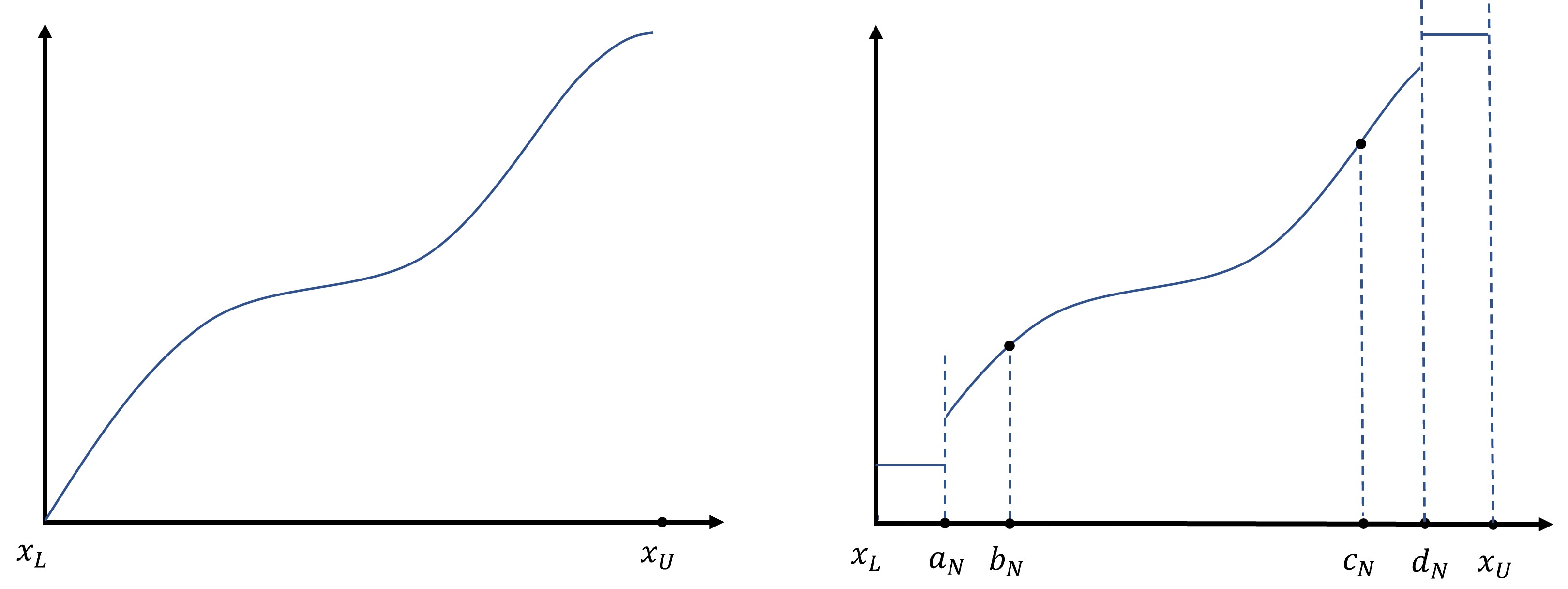
Figure 1. UC-isotonic estimator

The left panel is $p(x)$, and the right panel is $p_{N}(x)$.

The conclusion of Theorem 1 follows by showing these steps.

Step 1: $\sup_{x\in[x_{L},a_{N}]}|\tilde{p}(x)-p(x)|=O_{p}(N^{-1/3})$ and $\sup_{x\in[d_{N},x_{U}]}|\tilde{p}(x)-p(x)|=O_{p}(N^{-1/3}).$

Step 2: $\sup_{x\in[b_{N},c_{N}]}|\tilde{p}(x)-p(x)|=O_{p}\left(\frac{\log N}{N}\right)^{1/3}.$

Step 3: $\sup_{x\in(a_{N},b_{N})}|\tilde{p}(x)-p(x)|=O_{p}\left(\frac{\log N}{N}\right)^{1/3}$ and $\sup_{x\in(c_{N},d_{N})}|\tilde{p}(x)-p(x)|=O_{p}\left(\frac{\log N}{N}\right)^{1/3}.$

Step 1

Note that $\tilde{p}(a_{N})=\tilde{p}(x)$ for each $x\in[x_{L},a_{N}]$. Therefore, for $\sup_{x\in[x_{L},a_{N}]}|\tilde{p}(x)-p(x)|=O_{p}(N^{-1/3})$, it is enough to show that

$$\sup_{x\in[x_{L},a_{N}]}|\tilde{p}(a_{N})-p(x)|=O_{p}(N^{-1/3}).$$

First, by Assumption 2(iii) and Proposition 3(iii), we have $a_{N}-x_{L}=O_{p}(N^{-1/3}),$which implies

$$x-x_{L}=O_{p}(N^{-1/3})\text{ for }x\in[x_{L},a_{N}].$$ (37)

Thus, we have

$$\tilde{p}(a_{N}) = \frac{1}{N_{1}}\sum_{i=1}^{N_{1}}W_{i}=\frac{1}{c_{1}N^{2/3}}\sum_{i=1}^{c_{1}N^{2/3}}W_{i}$$

$$= \frac{\int_{x_{L}}^{q_{c_{1}\cdot N^{-1/3}}}p(x)f(x)dx}{\int_{x_{L}}^{q_{c_{1}\cdot N^{-1/3}}}f(x)dx}+O_{p}((c_{1}N^{2/3})^{-1/2})+O_{P}(N^{-1/2})$$

$$= \frac{\int_{x_{L}}^{q_{c_{1}\cdot N^{-1/3}}}\{p(x_{L})+p^{(1)}(x_{L})\cdot(x_{c_{1}}-x_{L})\}f(x)dx}{\int_{x_{L}}^{q_{c_{1}\cdot N^{-1/3}}}f(x)dx}+O_{p}(N^{-1/3})$$

$$= p(x_{L})+O_{p}(c_{1}\cdot N^{-1/3})+O_{p}(N^{-1/3})$$

$$= p(x)+O_{p}(N^{-1/3})+O_{p}(c_{1}\cdot N^{-1/3})+O_{p}(N^{-1/3})$$

$$= p(x)+O_{p}(N^{-1/3}),$$

where the first equality follows from Proposition 3(ii), the $O_{P}(N^{-1/2})$ term in the third equality follows from that $X_{c_{1}N^{2/3}}$ can estimate $q_{c_{1}\cdot N^{-1/3}}$ at the rate of $O_{P}(N^{-1/2})$, $x_{c_{1}}$ in the fourth equality is a number within the interval $(x_{L},q_{c_{1}\cdot N^{-1/3}})$, the fifth equality follows from $x_{c_{1}}-x_{L}=O_{p}(c_{1}\cdot N^{-1/3})$, the sixth equality follows from (37) and Assumption 2, and the last equality follows from $c_{1}=O_{p}(1)$, which is implied by (36).

Similarly, we can show $\sup_{x\in[d_{N},x_{U}]}|\tilde{p}(x)-p(x)|=O_{p}(N^{-1/3}).$

Step 2

The result $\sup_{x\in[b_{N},c_{N}]}|\tilde{p}(x)-p(x)|=O_{p}\left(\frac{\log N}{N}\right)^{1/3}$ follows by Durot, Kulikov, and Lopuhaä, (2013, Theorem 2.1). We can adapt the support from $[0,1]$ in their theorem to $[x_{L},x_{U}]$ in our problem, and their conditions (A1)-(A3) hold under Assumptions 1 and 2.

Step 3

The statement follows directly by combining the results from Steps 1 and 2 with Assumption 2, $b_{N}-a_{N}=O_{p}(N^{-1/3})$, and $d_{N}-c_{N}=O_{p}(N^{-1/3})$.

Combining these steps, the conclusion of this theorem follows.

A.5. Proof of Theorem 2

If $X_{i}$ is in the $k$-th partition given by the UC-isotonic estimator (i.e., $i\in\{n_{k},\ldots,(n_{k}+N_{k}-1)\}$), then we have $M_{i}=N_{k,1-W_{i}}$. Thus, the matching estimator $\hat{\tau}$ is written as

$$\hat{\tau} = \frac{1}{N}\sum_{i=1}^{N}(2W_{i}-1)\left(Y_{i}-\frac{1}{M_{i}}\sum_{j\in\mathcal{J}(i)}Y_{j}\right)=\frac{1}{N}\sum_{k=1}^{K}\left\{\sum_{i=n_{k}}^{n_{k}+N_{k}-1}(2W_{i}-1)\left(Y_{i}-\frac{1}{N_{k,1-W_{i}}}\sum_{j\in\mathcal{J}(i)}Y_{j}\right)\right\}$$ (38)

$$= \frac{1}{N}\sum_{k=1}^{K}\left\{\sum_{i\in\{n_{k},\ldots,(n_{k}+N_{k}-1)\},W_{i}=1}\left(Y_{i}-\frac{1}{N_{k,0}}\sum_{j\in\{n_{k},\ldots,(n_{k}+N_{k}-1)\},W_{j}=0}Y_{j}\right)\right.$$

$$\qquad\left.+\sum_{i\in\{n_{k},\ldots,(n_{k}+N_{k}-1)\},W_{i}=0}\left(\frac{1}{N_{k,1}}\sum_{j\in\{n_{k},\ldots,(n_{k}+N_{k}-1)\},W_{j}=1}Y_{j}-Y_{i}\right)\right\}$$

$$= \frac{1}{N}\sum_{k=1}^{K}\left\{\left(1+\frac{N_{k,0}}{N_{k,1}}\right)\sum_{i\in\{n_{k},\ldots,(n_{k}+N_{k}-1)\},W_{i}=1}Y_{i}-\left(\frac{N_{k,1}}{N_{k,0}}+1\right)\sum_{i\in\{n_{k},\ldots,(n_{k}+N_{k}-1)\},W_{i}=0}Y_{i}\right\}$$

$$= \frac{1}{N}\sum_{k=1}^{K}\left\{\frac{N_{k,1}+N_{k,0}}{N_{k,1}}\sum_{i\in\{n_{k},\ldots,(n_{k}+N_{k}-1)\},W_{i}=1}Y_{i}-\frac{N_{k,1}+N_{k,0}}{N_{k,0}}\sum_{i\in\{n_{k},\ldots,(n_{k}+N_{k}-1)\},W_{i}=0}Y_{i}\right\}$$

$$= \frac{1}{N}\sum_{k=1}^{K}\left\{\sum_{i\in\{n_{k},\ldots,(n_{k}+N_{k}-1)\},W_{i}=1}\frac{Y_{i}}{N_{k.1}/N_{k}}-\sum_{i\in\{n_{k},\ldots,(n_{k}+N_{k}-1)\},W_{i}=0}\frac{Y_{i}}{N_{k.0}/N_{k}}\right\}$$

$$= \frac{1}{N}\sum_{k=1}^{K}\left\{\sum_{i\in\{n_{k},\ldots,(n_{k}+N_{k}-1)\}}\left(\frac{W_{i}Y_{i}}{\tilde{p}(X_{i})}-\frac{\left(1-W_{i}\right)Y_{i}}{1-\tilde{p}(X_{i})}\right)\right\}$$

$$= \frac{1}{N}\sum_{i=1}^{N}\left(\frac{W_{i}Y_{i}}{\tilde{p}(X_{i})}-\frac{\left(1-W_{i}\right)Y_{i}}{1-\tilde{p}(X_{i})}\right),$$

where the first equality is the formula of matching estimator for ATE (see, e.g., Abadie and Imbens, 2016), with a changing matched set of size $M_{i}$, the fourth equality follows from the fact that with $w\in\{0,1\}$ and $i\neq j$, we have $\sum_{i\in n_{k}:(n_{k}+N_{k}-1),W_{i}=w}Y_{j}=N_{k,w}\cdot Y_{j}$, the second last equality follows from Lemma 3, and the last equality follows from $\sum_{k=1}^{K}N_{k}=N$.

A.6. Proof of Theorem 3

Theorem 3 follows from Theorem 2 and Xu (2021), where generic results for semiparametric estimation with plug-in isotonic estimator were given and applied to the case of IPW estimator. The proof will be decomposed into the following steps:

In Appendix A.6.1, we summarize the generic results for semiparametric estimation with plug-in (standard) isotonic estimator discussed in Xu (2021), and introduce relevant assumptions and lemmas. Their proofs are in Appendix A.6.2.

Appendix A.6.3 shows that the results in Appendix A.6.1 also hold for the plug-in UC-isotonic estimator. Then, we show the asymptotic properties of the IPW with plug-in UC-isotonic estimator and conclude the proof.

A.6.1. Relevant results on semiparametric estimation with plug-in isotonic estimator

We start by introducing several assumptions, lemma, theorem, and corollary. Other than in the main paper, the sample size is denoted by $n$ (not $N$) in this and next subsections.

Suppose we have a moment condition

$$\mathbb{E}[m(Z,\beta_{0},p_{0}(\cdot))] =0,$$ (39)

where $Z$ is a random vector defined on a probability space $(\Omega,\mathcal{B},\mathbb{P}_{0})$, and $\beta_{0}\in\mathfrak{B}\subset\mathbb{R}^{k}$ is a real-valued parameter of interest. $p_{0}(\cdot)$ is a monotone increasing nuisance function, which is the conditional mean of some function of data. Suppose we have the just identification, i.e., $\text{dim}(m(\cdot,\cdot,\cdot))=\text{dim}(\beta_{0})=k$. We are aiming at showing the properties of an estimator $\hat{\beta}$ solved from

$$\frac{1}{n}\sum_{i=1}^{n}m(Z_{i},\hat{\beta},\hat{p}(\cdot))=0.$$ (40)

where $Z_{i}$ is a vector of $i$-th observed data point, $\hat{p}(x)$ is a plug-in isotonic estimator of $\mathbb{E}[Y|X=x]$. $(Y,X)$ is a sub-vector of $Z$. Note that $Y$ here are no longer defined as outcomes, but the dependent variable of an isotonic regression, and it corresponds the treatment $W$ in the main paper. In the general setting, $Y$ can be both binary or continuous. To proceed, we impose the following assumptions.

A1:

$X$ is a random scalar taking value in the space $\mathcal{X}$. The space $\mathcal{X}$ is convex with non-empty interiors, and satisfies $\mathcal{X}\subset\mathcal{B}(0,R)$ for some $R>0$.

A2:

$\mathbb{E}[Y|X=x]=p_{0}(x)$ is monotone increasing in $x$. There exists $K_{0}>0$ such that $|p_{0}(x)|<K_{0}$ for all $x\in\mathcal{X}$.

A3:

There exist $c_{0}>0$ and $M_{0}>0$ such that $\mathbb{E}[|Y|^{m}|X=x]\leq m!M_{0}^{m-2}c_{0}$ for all integers $m\geq 2$ and almost every $x$.

A1 and A2 impose boundedness on the monotone function $p_{0}$ and the support of $X$. These conditions are used to control the entropy of the function classes that characterize (40). A3 is to restrict the size of the tail of $Y|X$. With A3, we can show that $\underset{x\in X}{\text{sup }}\hat{p}(x)=O_{p}(\log n)$, which is used to obtain an entropy result associated with the $\sqrt{n}$-convergence rate in the second-stage semiparametric estimator.

Lemma 2.

Let $\hat{p}(\cdot)$ be an isotonic estimator of $\mathbb{E}[Y|X]$, and $\delta(X)$ be a bounded function of $X$ with a finite total variation. Under A1, A2, and A3, we have

$$\frac{1}{n}\sum_{i=1}^{n}\delta(X_{i})(Y_{i}-\hat{p}(X_{i}))=o_{p}(n^{-1/2}).$$ (41)

Let $D(z,\beta)$ be the functional derivative of $m(z,\beta,p(x))$ with respect to $p(\cdot)$. We assume:

A4:

For all $\beta\in\mathfrak{B}$, $\mathbb{E}[D(Z,\beta)|X]$ is a bounded function of $X$ with a finite total variation, and there exist $c_{1}>0$ and $M_{1}>0$ such that for each row of $D(Z,\beta)$ ($D_{j}(Z,\beta)$ with $j\in\{1:k\}$), $\mathbb{E}[|D_{j}(Z,\beta)|^{m}|X=x]\leq m!M_{1}^{m-2}c_{1}$ for all integers $m\geq 2$ and almost every $x$.

By (41), we have

$$\frac{1}{n}\sum_{i=1}^{n}\mathbb{E}[D(Z_{i},\beta_{0})|X_{i}](Y_{i}-\hat{p}(X_{i}))=o_{p}(n^{-1/2}).$$

Then we add the following assumption:

A5:

The first-order expansion of $m(z,\beta,p(\cdot))$ with respect to $p(\cdot)$ at $p^{*}(\cdot)$, $D(z,\beta,p(\cdot)-p^{*}(\cdot))$, is linear in $p(\cdot)-p^{*}(\cdot)$ (i.e., $D(z,\beta,p(x)-p^{*}(x))=D(z,\beta)\{p(x)-p^{*}(x)\}$).

The correction term $\mathbb{E}[D(Z,\beta_{0})|X]\{Y-p_{0}(X)\}$ is also associated with efficiency. As illustrated in Newey (1994, Proposition 4), for unconditional moment condition $\mathbb{E}[m(Z,\beta,p(X))]=0$, where $p_{0}(X)=\mathbb{E}[Y|X]$ for some sub-vector $Y$, the efficient influence function $\psi$ is

$$\psi(Z)=-\left(\frac{\partial\mathbb{E}[m(Z,\beta_{0},p(X))]}{\partial\beta}\right)^{-1}[m(Z,\beta_{0},p_{0}(X))+\mathbb{E}[D(Z,\beta_{0})|X]\{Y-p_{0}(X)\}].$$

If we could show for an isotonic plug-in estimator $\hat{p}(\cdot)$

$$\frac{1}{n}\sum_{i=1}^{n}m(Z_{i},\beta_{0},\hat{p}(X_{i}))=\frac{1}{n}\sum_{i=1}^{n}\{m(Z_{i},\beta_{0},p_{0}(x_{i}))+\mathbb{E}[D(Z,\beta_{0})|X_{i}](y_{i}-p_{0}(x_{i}))\}+o_{p}(n^{-1/2}),$$

we could show the asymptotic efficiency. To this end, we impose the following assumptions:

A6:

There are $b(z)>0$ and $D(z,g)$ that (i) $||m(z,\beta,p)-m(z,\beta,p_{0})-D(z,\beta,p-p_{0})||\leq b(z)||p-p_{0}||^{2}$; (ii) $\mathbb{E}[b(Z)]=o_{p}(n^{1/6}(\log n)^{-2})$, for all $\beta\in\mathfrak{B}$, where $\mathfrak{B}$ is compact.

A7:

There are $\varepsilon$, $b(z)$, $\tilde{b}(z)>0$ and $p(\cdot)$ with $||p||>0$. Such that (i) for all $\beta\in\mathfrak{B}$, $m(z,\beta,p_{0})$ is continuous at $\beta$ and $m(z,\beta,p_{0})\leq b(z)$; (ii) $||m(z,\beta,p)-m(z,\beta,p_{0})||\leq\tilde{b}(z)(||p-p_{0}||)^{\varepsilon}$.

A8:

$\mathbb{E}[m(z,\beta,p_{0})]=0$ has a unique solution on $\mathfrak{B}$ at $\beta_{0}$.

A9:

For $\beta\in\text{interior}(\mathfrak{B})$, (i) there are $\varepsilon>0$ and a neighborhood $\mathscr{N}$ of $\beta_{0}$ such that for all $||p-p_{0}||\leq\varepsilon$, $m(z,\beta,p)$ is differentiable in $\beta$ on $\mathscr{N}$; (ii) $M_{\beta}=-\mathbb{E}\left[\frac{\partial m(Z,\beta_{0},p_{0}(X))}{\partial\beta}\right]$ is nonsingular; (iii) $\mathbb{E}[||m(z,\beta,p)||^{2}]<\infty$; (iv) Assumption A7 is satisfied with $m(z,\beta,p)$ equaling to each row of $\frac{\partial m(Z,\beta,p)}{\partial\beta}$.

A6 is an adaption of Assumption 5.1 in Newey (1994). This assumption requires that the higher order term from a linear approximation is small. A7, A8, and A9 are adapted from Assumption 5.4, 5.5, and 5.6 in Newey (1994). They are general conditions for the consistency and asymptotical normality of the method of moment estimator.

Define $M(Z)=\mathbb{E}[D(Z,\beta_{0})|X](Y-p_{0}(X))$. The asymptotic normality and efficiency of the plug-in estimator $\hat{\beta}$ is obtained as follows.

Lemma 3.

Let $\hat{p}(\cdot)$ be an isotonic estimator of $p_{0}(\cdot)=\mathbb{E}[Y|X=\cdot]$. Under A1-A9, it holds

$$\sqrt{n}(\hat{\beta}-\beta_{0})\overset{d}{\to}N(0,V),$$

where $V=M_{\beta}^{-1}\mathbb{E}[\{m(Z,\beta_{0},p_{0})+M(Z)\}\{m(z,\beta_{0},p_{0})+M(Z)\}^{\prime}]M_{\beta}^{-1}$.

A.6.2. Proofs of the results in Appendix A.6.1

Proof of Lemma 2

The proof here is based on the supplementary material of BGH (hereafter BGH-supp). Similar techniques can also be found in Groeneboom and Jongbloed (2014) and Groeneboom and Hendrickx (2018). For isotonic estimator $\hat{p}(\cdot)$, we have

$$||\hat{p}-p_{0}||^{2}=O_{p}((\log n)^{2}n^{-2/3})=o_{p}(n^{-1/2}),$$ (42)

(see, e.g., Theorem 9.2 and Lemma 5.15 in van de Geer, S., 2000).

Let $\{x_{n_{j}}\}_{j=1}^{k}$ be the subsequence of $\{x_{i}\}_{i=1}^{n}$ representing all the jump points of $\hat{p}(\cdot)$. By the construction of $\hat{p}(\cdot)$ (see, e.g., Lemmas 2.1 and 2.3 in Groeneboom and Jongbloed, 2014), we have $\sum_{i=n_{j}}^{n_{j+1}-1}\{y_{i}-\hat{p}(x_{i})\}=0$ for each $j=1,\ldots,k$, which implies

$$\sum_{j=1}^{k}m_{j}\sum_{i=n_{j}}^{n_{j+1}-1}\{y_{i}-\hat{p}(x_{i})\}=0,$$ (43)

for any weights $\{m_{j}\}_{j=1}^{k}$. Define the step function

$$\bar{\delta}_{n}(x)=\begin{cases}\delta(x_{n_{j}})&\text{if }p_{0}(x)>\hat{p}(x_{n_{j}})\text{ for all }x\in(x_{n_{j}},x_{n_{j+1}})\\ \delta(s)&\text{if }p_{0}(s)=\hat{p}(s)\text{ for some }s\in(x_{n_{j}},x_{n_{j+1}})\\ \delta(x_{n_{j+1}})&\text{if }p_{0}(x)<\hat{p}(x_{n_{j}})\text{ for all }x\in(x_{n_{j}},x_{n_{j+1}})\end{cases},$$

for $x\in[x_{n_{j}},x_{n_{j+1}})$ with $j=1,\ldots,k$ (if $j=k$, set $x_{n_{j+1}}=\text{$\underset{i}{\text{max }}$}x_{n_{i}}$). By (43), it holds $\int\bar{\delta}_{n}(x)\{y-\hat{p}(x)\}d\mathbb{P}_{n}(z)=0$, and thus

$$\frac{1}{n}\sum_{i=1}^{n}\delta(X_{i})(Y_{i}-\hat{p}(X_{i}))=\int\delta(x)\{y-\hat{p}(x)\}d\mathbb{P}_{n}(z)=\int[\delta(x)-\bar{\delta}_{n}(x)](y-\hat{p}(x))d\mathbb{P}_{n}(z).$$ (44)

By assumption, $\delta(x)$ is a bounded function with a finite total variation, so is $\bar{\delta}_{n}(x)$. Therefore, by a similar argument as in pp. 18-20 of BGH-supp, we have $\int[\delta(x)-\bar{\delta}_{n}(x)](y-\hat{p}(x))d\mathbb{P}_{n}(z)=o_{p}(n^{-1/2})$. We see that (44) can be decomposed as

$$\int[\delta(x)-\bar{\delta}_{n}(x)](y-\hat{p}(x))d\mathbb{P}_{n}(z) = \int[\delta(x)-\bar{\delta}_{n}(x)](y-\hat{p}(x))d\{\mathbb{P}_{n}(z)-\mathbb{P}_{0}(z)\}$$

$$+\int[\delta(x)-\bar{\delta}_{n}(x)](y-p_{0}(x))d\mathbb{P}_{0}(z)$$

$$+\int[\delta(x)-\bar{\delta}_{n}(x)](p_{0}(x)-\hat{p}(x))d\mathbb{P}_{0}(z)$$

$$= I+II+III.$$

By Lemma 21 in BGH-supp, $\delta(x)-\bar{\delta}_{n}(x)$ are bounded functions with finite total variations. By similar arguments in Groeneboom and Jongbloed (2014), there exists a positive constant $C_{0}$ such that for all $x\in\mathcal{X}$,

$$|\delta(x)-\bar{\delta}_{n}(x)|\leq C_{0}|p_{0}(x)-\hat{p}(x)|.$$ (45)

For $I$, let us define the following function classes

$$\mathcal{M}_{RK} = \{\text{monotone increasing functions on $[-R,R]$ and bounded by $K$}\},$$

$$\mathcal{G}_{RK} = \{g:g(x)=p(x),x\in\mathcal{X},p\in\mathcal{M}_{RK}\},$$

$$\mathcal{D}_{RKv} = \{d:d(x)=g_{1}(x)-g_{2}(x),\text{ }(g_{1},g_{2})\in\mathcal{\mathcal{G}}_{RK}^{2},\text{ }||d(x)||_{P_{0}}\leq v\},$$

$$\mathcal{H}_{RKv} = \{h:h(y,x)=yd_{1}(x)-d_{2}(x),\text{ }(d_{1},d_{2})\in\mathcal{D}_{RKv}^{2},\text{ }z\in\mathcal{Z}\}.$$ (46)

The integrand of $I$ is written as

$$[\delta(x)-\bar{\delta}_{n}(x)](y-\hat{p}(x))=[\delta(x)-\bar{\delta}_{n}(x)]y-[\delta(x)-\bar{\delta}_{n}(x)]\hat{p}(x).$$ (47)

Let $\mathcal{F}_{a}=\{f:f(z)=[\delta(x)-\bar{\delta}_{n}(x)]y-[\delta(x)-\bar{\delta}_{n}(x)]\hat{p}(x),\text{ }z\in\mathcal{Z}\}$. We observe the following facts:

(i) By Lemma 21 in BGH-supp, $\delta(x)-\bar{\delta}_{n}(x)$ is a bounded function of $x$ with finite total variation.

(ii) By Assumption A3, we can show $\sup_{x\in\mathcal{X}}|\hat{p}(x)|=O_{p}(\log n)$ (see, e.g., Lemma 7.1 in Balabdaoui, Durot, and Jankowski, 2019). Therefore, there exists $K_{1}>0$, such that $\hat{p}(x)\in\mathcal{G}_{R(K_{1}\log n)}$ with probability approaching one.

(iii) By (42) and (45), we have $||\delta(x)-\bar{\delta}_{n}(x)||_{2}\leq C_{1}(\log n)n^{-1/3}$, for some $C_{1}>0$. Thus, there exists a positive constant $C_{2}$ that is larger than twice the bound of $\delta(x)$, and $v_{1}=C_{1}(\log n)n^{-1/3}$, such that $[\delta(x)-\bar{\delta}_{n}(x)]\in\mathbb{\mathcal{D}}_{RC_{2}v_{1}}$.

(iv) By (ii), a similar argument of (iii), (42), and Jensen’s inequality, we have $[\delta(x)-\bar{\delta}_{n}(x)]\hat{p}(x)\in\mathcal{D}_{R(K_{2}\log n)v_{2}}$ for a large enough constant $K_{2}>0$ and $v_{2}=C_{3}(\log n)^{2}n^{-1/3}$ for some $C_{3}>0$, with probability approaching one.

We choose $K=\text{max}\{C_{2},K_{2}\log n\}$ and $v=\text{max}\{v_{1},v_{2}\}$. Now we have (47)$\in\mathcal{H}_{RKv}$.

Define $||\mathbb{G}_{n}||_{\mathcal{F}}=\sup_{f\in\mathcal{F}}|\sqrt{n}(\mathbb{P}_{n}-P_{0})f|$. Let $N_{[]}(\varepsilon,\mathcal{F},||\cdot||)$ be the $\varepsilon$-bracketing number of the function class $\mathcal{F}$ under the norm $||\cdot||$, and $H_{B}(\varepsilon,\mathcal{F},||\cdot||)=\text{log}N_{[]}(\varepsilon,\mathcal{F},||\cdot||)$ be the entropy of $N_{[]}(\varepsilon,\mathcal{F},||\cdot||)$, and $J_{n}(\delta,\mathcal{F},||\cdot||)=\int_{0}^{\delta}\sqrt{1+H_{B}(\varepsilon,\mathcal{F},||\cdot||)}d\varepsilon$. Let $||\cdot||_{B,P_{0}}$ be the Bernstein norm under a measure $P_{0}$. In this section, we use $J_{n}(\delta)$ to denote $J_{n}(\delta,\mathcal{F},||\cdot||_{B,P_{0}})$. By similar arguments in Lemma 13 of BGH-supp (in our case, we can ignore the single-index coefficients), we have, with probability approaching one:

$$H_{B}(\varepsilon,\tilde{\mathcal{F}}_{a},||\cdot||_{B,P_{0}})\leq\frac{C_{3}}{\varepsilon},$$ (48)

for some $C_{3}>0$, where $\tilde{\mathcal{F}}_{a}=(C_{4}\log n)^{-1}\mathcal{F}_{a}$ with some $C_{4}>0$. Also, there exists a constant $C_{5}>0$ such that

$$||\tilde{f}||_{B,P_{0}}\leq C_{5}(\log n)n^{-1/3},$$ (49)

for all $\tilde{f}_{a}\in\tilde{\mathcal{F}_{a}}$, with probability approaching one. We use $\mathscr{E}$ to denote the event that both (48) and (49) happen, and we have $\underset{n\to\infty}{\text{lim}}P(\mathscr{E})=1$.

Let $\delta_{n}=C_{5}(\log n)n^{-1/3}$ and $I_{j}$ be the $j$-th component of $I$. For any positive constants $A$ and $\nu$, there exist positive constants $B_{1}$, and $B_{2}$ such that

$$\mathbb{P}\{|I_{j}|>An^{-1/2}\} \leq \mathbb{P}\left\{|I_{j}|>An^{-1/2},\mathscr{E}\right\}+P(\mathscr{E}^{c})\leq\mathbb{P}\left\{||\mathbb{G}_{n}||_{\mathcal{F}_{a}}>A,\mathscr{E}\right\}+\frac{\nu}{2}$$ (50)

$$\leq \frac{\mathbb{E}[||\mathbb{G}_{n}||_{\mathcal{F}_{a}}\quad|\mathscr{E}]}{A}+\frac{\nu}{2}=\frac{C_{4}\log n}{A}\mathbb{E}[||\mathbb{G}_{n}||_{\tilde{\mathcal{F}}_{a}}\quad|\mathscr{E}]+\frac{\nu}{2}$$

$$\lesssim \frac{C_{4}\log n}{A}J_{n}(\delta_{n})\left(1+\frac{J_{n}(\delta_{n})}{\sqrt{n}\delta_{n}^{2}}\right)+\frac{\nu}{2}$$

$$\lesssim \frac{\log n}{A}(\delta_{n}+2B_{1}^{1/2}\delta_{n}^{1/2})\left(1+\frac{\delta_{n}+2B_{1}^{1/2}\delta_{n}^{1/2}}{\sqrt{n}\delta_{n}^{2}}\right)+\frac{\nu}{2}$$

$$\lesssim \frac{1}{A}(\log n)^{3/2}n^{-1/6}\left(1+\frac{B_{2}}{(\log n)^{3/2}}\right)+\frac{\nu}{2}\lesssim\nu,$$

for all $n$ large enough, where the second inequality follows from the definition of $\mathcal{F}_{a}$, the third inequality follows from the Markov inequality, the first equality follows from the definition of $\tilde{\mathcal{F}}_{a}$, the first wave inequality ($\lesssim$) comes from Lemma 3.4.3 of van der Vaart and Wellner (1996) and the definition of $\delta_{n}$, the second wave inequality comes from (48) and Equation (.2) in BGH-supp, and the third wave inequality follows from $\delta_{n}\lesssim\delta_{n}^{1/2}$ and the definition of $\delta_{n}$. Therefore,

$$I=o_{p}(n^{-1/2}).$$ (51)

For $II$, the law of iterated expectation yields

$$II=\int[\delta(x)-\bar{\delta}_{n}(x)](y-p_{0}(x))d\mathbb{P}_{0}(z)=0.$$

For $III$, we have

$$III = \int[\delta(x)-\bar{\delta}_{n}(x)](p_{0}(x)-\hat{p}(x))d\mathbb{P}_{0}(z)\lesssim\int(p_{0}(x)-\hat{p}(x))^{2}d\mathbb{P}_{0}(z)$$

$$= O_{p}((\log)^{2}n^{-2/3})=o_{p}(n^{-1/2}),$$

where the first wave inequality follows from (45), and the second equality follows from (42).

Combining the rates for $I$, $II$, and $III$, the conclusion of Lemma 2 follows.

Proof of Lemma 3

The proof is a combination of the techniques for isotonic regression applied in Groeneboom and Hendrickx (2018) and BGH, and the framework of Newey (1994). Let $u=y-p_{0}(x)$ and $M(z)=\delta(x)u$. We verify Assumptions 5.1-5.6 of Newey (1994).

Step 1: Verify Assumption 5.1 of Newey (1994)

(i) There is a function $D(z,p)$ that is linear in $p$ such that for all $p$ with $||p-p_{0}||$ small enough, $||m(z,p)-m(z,p_{0})-D(z,p-p_{0})||\leq b(z)||p-p_{0}||^{2}$, and (ii) $\mathbb{E}(b(Z))\sqrt{n}||\hat{p}-p_{0}||^{2}\overset{p}{\to}0$.

Assumption 5.1(i) is a restatement of A6 (i). Assumption 5.1(ii) can be derived by A6(ii) and the fact $||\hat{p}-p_{0}||^{2}=O_{p}((\log n)^{2}n^{-2/3})$ (see, e.g., Theorem 9.2 and Lemma 5.15 in van de Geer, S., 2000).

Step 2: Verify Assumption 5.2 of Newey (1994).

It holds $\frac{1}{n}\sum_{i=1}^{n}D(Z_{i},\hat{p}(X_{i})-p_{0}(X_{i}))-\int D(z,\hat{p}(x)-p_{0}(x))d\mathbb{P}_{0}(z)=o_{p}(n^{-1/2})$.

By A5, we have

$$\frac{1}{n}\sum_{i=1}^{n}D(Z_{i},\beta_{0},\hat{p}(X_{i})-p_{0}(X_{i}))-\int D(z,\beta_{0},\hat{p}(x)-p_{0}(x))d\mathbb{P}_{0}(z)=\int D(z,\beta_{0})(p_{0}(x)-\hat{p}(x))d(\mathbb{P}_{n}-\mathbb{P}_{0})(z).$$ (52)

Let

$$\mathcal{F}_{b}=\{f:f(z)=D(z,\beta_{0})(p_{0}(x)-\hat{p}(x)),\text{ }x\in\mathcal{X}\}.$$

To avoid heavy notations, we re-define some constant terms in this subsection, such as $A_{i}$, $C_{i}$, $K_{i}$, $\delta_{n}$, and $v$, etc.. They are not related to those constants with the same names in other sections.

By similar arguments as in the proof of Lemma 2, for some $C_{1},C_{2}>0$, we have

$$p_{0}(x)-\hat{p}(x)\in\mathcal{D}_{R(C_{1}\text{log}n)(C_{2}n^{-1/3}\log n)},$$ (53)

with probability approaching one. By Theorem 2.7.5 in van der Vaart and Wellner (1996) and Lemma 11 in BGH-supp, with $R,C,v>0$, we have

$$H_{B}(\varepsilon,\mathcal{D}_{RCv},||\cdot||_{P_{0}})\leq\frac{AC}{\varepsilon},$$

for some $A>0$.

Now we define

$$\mathcal{H}_{RKv}^{(2)}=\{h:h(z)=D(z,\beta_{0})d(x),\text{ }d(\cdot)\in\mathcal{D}_{RKv},\text{ }z\in\mathcal{Z}\},$$

and let $D(z,\beta_{0})\in\mathbb{R}^{1}$. This is just to simplify the notation of the following proof, i.e., the following steps hold for any $D_{j}(z,\beta_{0})$ with $j\in\{1:k\}$, the $j$-th row of $D(z,\beta_{0})$. Let $(d^{L},d^{U})$ be any $\epsilon$-bracket of the function class $\mathcal{D}_{RKv}$, and

$$h^{L} = \begin{cases}D(z,\beta_{0})d^{L}(x)&\text{if }D(z,\beta_{0})\geq 0\\ D(z,\beta_{0})d^{U}(x)&\text{if }D(z,\beta_{0})<0\end{cases},$$

$$h^{U} = \begin{cases}D(z,\beta_{0})d^{U}(x)&\text{if }D(z,\beta_{0})\geq 0\\ D(z,\beta_{0})d^{L}(x)&\text{if }D(z,\beta_{0})<0\end{cases}.$$

We see that $(h^{L},h^{U})$ is a bracket of $h$ whose size is

$$\int_{\mathcal{Z}}\{h^{U}(z)-h^{L}(z)\}^{2}d\mathbb{P}_{0}(z) =\int_{\mathcal{Z}}D(z,\beta_{0})^{2}\{d^{U}(x)-d^{L}(x)\}^{2}d\mathbb{P}_{0}(z)$$

$$=\int_{\mathcal{X}}\mathbb{E}[D(z,\beta_{0})^{2}|x]\{d^{U}(x)-d^{L}(x)\}^{2}d\mathbb{P}_{0}(x)$$

$$=A_{1}\epsilon^{2},$$

for some $A_{1}>0$. The last equality follows from A4 and the definition of $\epsilon$-bracket. Thus, for some $\tilde{A}>0$, we have

$$H_{B}(\varepsilon,\mathcal{H}_{RCv}^{(2)},||\cdot||_{P_{0}})\leq\frac{\tilde{A}C}{\varepsilon}.$$ (54)

Now we switch to Bernstein norm since we do not want to put a bound on $D(z,\beta_{0})$. By the definition of Bernstein norm

$$||h||_{B,P_{0}}^{2}=2\mathbb{E}_{0}[\text{exp}(|h|)-|h|-1]=2\int\sum_{k=2}^{\infty}\frac{1}{k!}|h|^{k}d\mathbb{P}_{0}(z).$$

We bound the Bernstein norm of $\frac{h(\cdot)}{H}$, where $H$ is some positive constant chosen in the following steps to achieve a finite upper bound. Observe that

$$||H^{-1}h||_{B,P_{0}}^{2} = 2\int\sum_{k=2}^{\infty}\frac{1}{H^{k}}\frac{1}{k!}|D(z,\beta_{0})d(x)|^{k}d\mathbb{P}_{0}(z)\leq 2\int\sum_{k=2}^{\infty}\frac{1}{H^{k}}\frac{1}{k!}|D(z,\beta_{0})|^{k}|d(x)|^{k}d\mathbb{P}_{0}(z)$$

$$\leq 2\sum_{k=2}^{\infty}\frac{1}{H^{k}}\frac{(2C)^{k-2}}{k!}k!M_{1}^{k-2}c_{1}\int|d(x)|^{2}d\mathbb{P}_{0}(z)$$

$$= \frac{2}{H^{2}}\sum_{k=2}^{\infty}\frac{(2M_{1}C)^{k-2}}{H^{k-2}}c_{1}\int|d(x)|^{2}d\mathbb{P}_{0}(z)=\frac{2}{H^{2}}\sum_{k=2}^{\infty}\left(\frac{2M_{1}C}{H}\right)^{k-2}c_{1}v^{2}$$

$$= \left(\frac{2}{H}\right)^{2}c_{1}v^{2},$$

where the second inequality follows from A4 and the fact $d(\cdot)\in\mathcal{D}_{RCv}$, where $c_{1}$ and $M_{1}$ are the same constants in A4, the third equality follows from the definition of $v$ in $\mathcal{D}_{RCv}$, and the last equality follows by choosing $H=4M_{1}C$. This implies

$$||H^{-1}h||_{B,P_{0}}\lesssim H^{-1}v.$$ (55)

Now by setting $C=C_{1}\text{log}n$, $v=C_{2}n^{-1/3}\log n$ so that $\mathcal{F}_{b}\subset\mathcal{H}_{R(C_{1}\text{log}n)(C_{2}n^{-1/3}\log n)}^{(2)}$, and $\tilde{H}=4M_{1}C_{1}\text{log}n$, we have

$$\mathcal{\tilde{F}}_{b}=\tilde{H}^{-1}\mathcal{F}_{b}\quad\text{for some }C_{3}>0.$$

Thus, combining (54) and (55), it holds that with probability approaching one

$$H_{B}(\varepsilon,\tilde{\mathcal{F}}_{b},||\cdot||_{B,P_{0}})\leq\frac{C_{3}}{\varepsilon},$$ (56)

for some $C_{3}>0$, and

$$||\tilde{f}||_{B,P_{0}}\leq C_{4}n^{-1/3},$$ (57)

for all $\tilde{f}_{b}\in\tilde{\mathcal{F}_{b}}$ and some $C_{4}>0$.

We use $\mathscr{E}_{1}$ to denote the events defined in (56) and (57), and use $S$ to denote the value of (52). Let $\delta_{n}=C_{4}n^{-1/3}$. For any $A_{2}>0$, it holds

$$\mathbb{P}\{|S|>A_{2}n^{-1/2}\} \leq \mathbb{P}\{|S|>A_{2}n^{-1/2},\mathscr{E}_{1}\}+\mathbb{P}\{\mathscr{E}_{1}^{c}\}\leq\mathbb{P}\{||\mathbb{G}_{n}||_{\mathcal{F}_{b}}>A_{2},\mathscr{E}_{1}\}+\frac{\nu}{2}$$ (58)

$$\leq \frac{\mathbb{E}[||\mathbb{G}_{n}||_{\mathcal{F}_{b}}|\mathscr{E}_{1}]}{A_{2}}+\frac{\nu}{2}\lesssim\frac{\log n}{A_{2}}\mathbb{E}[||\mathbb{G}_{n}||_{\tilde{\mathcal{F}}_{b}}|\mathscr{E}_{1}]+\frac{\nu}{2}$$

$$\lesssim \frac{\log n}{A_{2}}J_{n}(\delta_{n})\left(1+\frac{J_{n}(\delta_{n})}{\sqrt{n}\delta_{n}^{2}}\right)+\frac{\nu}{2}\lesssim\frac{\log n}{A_{2}}(\delta_{n}+2B_{1}^{1/2}\delta_{n}^{1/2})\left(1+\frac{\delta_{n}+2B_{1}^{1/2}\delta_{n}^{1/2}}{\sqrt{n}\delta_{n}^{2}}\right)+\frac{\nu}{2}$$

$$\lesssim \frac{1}{A}(\log n)^{3/2}n^{-1/6}\left(1+\frac{B_{2}}{(\log n)^{3/2}}\right)+\frac{\nu}{2}\lesssim\frac{\log n}{A_{2}}n^{-1/6}B_{2}+\frac{\nu}{2}$$

$$\lesssim \nu.$$

These steps are similar to those of (50). Thus, we have $\int D(z,\beta_{0})\{p_{0}(x)-\hat{p}(x)\}d(\mathbb{P}_{n}-\mathbb{P}_{0})(z)=o_{p}(n^{-1/2})$ and Assumption 5.2 in Newey (1994) is satisfied.

Step 3: Verify Assumption 5.2 of Newey (1994).

It holds $\int D(z,\hat{p}(x)-p_{0}(x))d\mathbb{P}_{0}(z)=\frac{1}{n}\sum_{i=1}^{n}M(Z_{i})+o_{p}(n^{-1/2})$.

Note that

$$\int D(z,\beta_{0},\hat{p}(x)-p_{0}(x))d\mathbb{P}_{0}(z) = \int D(z,\beta_{0})(\hat{p}(x)-p_{0}(x))d\mathbb{P}_{0}(x)$$

$$= \int\mathbb{E}(D(Z,\beta_{0})|X=x)(\hat{p}(x)-p_{0}(x))d\mathbb{P}_{0}(x)$$

$$= \int\delta(x)(\hat{p}(x)-p_{0}(x))d\mathbb{P}_{0}(x),$$

where the first equality follows from A5, and the last equality follows by setting $\mathbb{E}[D(Z,\beta_{0})|X=x]=\delta(x)$. By plugging in $M(z)=\delta(x)u$, we obtain

$$\int D(z,\hat{p}(x)-p_{0}(x))d\mathbb{P}_{0}(z)-\frac{1}{n}\sum_{i=1}^{n}M(Z_{i})$$ (59)

$$= \int\delta(x)(\hat{p}(x)-p_{0}(x))d\mathbb{P}_{0}(x)-\frac{1}{n}\sum_{i=1}^{n}\delta(X_{i})(Y_{i}-p_{0}(X_{i}))$$

$$= \int\delta(x)(\hat{p}(x)-p_{0}(x))d\mathbb{P}_{0}(x)-\int\delta(x)(y-\hat{p}(x)+\hat{p}(x)-p_{0}(x))d\mathbb{P}_{n}(z)$$

$$= \int-\delta(x)(y-\hat{p}(x))d\mathbb{P}_{n}(z)+\int-\delta(x)(\hat{p}(x)-p_{0}(x))d(\mathbb{P}_{n}-\mathbb{P}_{0})(x)$$

$$= I+II.$$

Lemma 2 guarantees $I=o_{p}(n^{-1/2})$. For $II$, by A4 and a similar argument as in p. 23 of BGH-supp, we have $II=o_{p}(n^{-1/2})$. Thus, Assumption 5.3 in Newey (1994) is satisfied.

Step 4: Conclude the proof

Assumptions 5.4-5.6 in Newey (1994) are adapted as A7-A9 in this paper. Therefore, all the assumptions in Newey (1994, Assumptions 5.1-5.6) are satisfied in our setup.

Now the consistency can be proved by similar arguments as in Lemma 5.2 of Newey (1994). Also by Lemma 5.3 of Newey (1994), we obtain $\sqrt{n}(\hat{\beta}-\beta_{0})\overset{d}{\to}N(0,V)$. Finally, the asymptotic efficiency is proved according to Proposition 4 of Newey (1994).

A.6.3. Asymptotic properties of $\hat{\tau}$

The results in Appendix A.6.1 also hold for the UC-isotonic estimator $\tilde{p}(\cdot)$. Recall that in Appendices A.6.1 and A.6.2, $Y$ represents the dependent variable of isotonic regression, and for the sample size $n$, $\tilde{p}(\cdot)$ is obtained by regression $\tilde{Y}$ on $X$, where

$$\tilde{Y}_{i}=\begin{cases}\frac{1}{\lfloor n^{2/3}\rfloor}\sum_{i=1}^{\lfloor n^{2/3}\rfloor}Y_{i}&\text{for }i\leq\lfloor n^{2/3}\rfloor\\ Y_{i}&\text{for }\lfloor n^{2/3}\rfloor<i\leq n-\lfloor n^{2/3}\rfloor\\ \frac{1}{\lfloor n^{2/3}\rfloor}\sum_{i=n-\lfloor n^{2/3}\rfloor+1}^{N}Y_{i},&\text{for }i>n-\lfloor n^{2/3}\rfloor\end{cases}$$

where the ordering is according to $X_{1}<X_{2}<\dots<X_{n}$.

Lemma 4.

Let $\tilde{p}(\cdot)$ be the UC-isotonic estimator of the conditional mean $\mathbb{E}[Y|X]$, and $\delta(X)$ be a bounded function of $X$ with a finite total variation. Under A1, A2, and A3, it holds

$$\frac{1}{n}\sum_{i=1}^{n}\delta(X_{i})(Y_{i}-\tilde{p}(X_{i}))=o_{p}(n^{-1/2}).$$ (60)

Proof.

Note that two key results, (42) and (43) also hold for $\tilde{p}(\cdot)$:

$$||\tilde{p}-p_{0}||^{2} =O_{p}\left[\left(\frac{\log n}{n}\right)^{2/3}\right]=o_{p}(n^{-1/2}),$$ (61)

$$\sum_{j=1}^{k}m_{j} \sum_{i=n_{j}}^{n_{j+1}-1}\{Y_{i}-\tilde{p}(\cdot)\}=0,$$ (62)

where (61) follows from Theorem 1, and (62) is by Proposition 3(i). Based on (61) and (62), all other arguments in the proof of Lemma 2 in Appendix A.6.2 hold for the UC-isotonic estimator $\tilde{p}(\cdot)$. ∎

As a result, Lemma 3 also holds for $\tilde{p}(\cdot)$, which is presented as follows.

Lemma 5.

Let $\tilde{p}(\cdot)$ be the UC-isotonic estimator of the conditional mean $\mathbb{E}[Y|X]$, and $\tilde{\beta}$ be the solution of the moment condition $\frac{1}{n}\sum_{i=1}^{n}m(Z_{i},\tilde{\beta},\tilde{p}(\cdot))=0$. Under A1-A9, it holds

$$\sqrt{n}(\tilde{\beta}-\beta_{0})\overset{d}{\to}N(0,V),$$

where $V=M_{\beta}^{-1}\mathbb{E}[\{m(Z,\beta_{0},p_{0})+M(Z)\}\{m(z,\beta_{0},p_{0})+M(Z)\}^{\prime}]M_{\beta}^{-1}$.

We apply Lemma 5 to the ATE model by setting $Z=(Y,W,X)$, $\beta_{0}=\mathbb{E}\left[\frac{Y\cdot W}{p_{0}(X)}-\frac{Y\cdot(1-W)}{1-p(X)}\right]$, $m(Z,\beta,p(\cdot))=\frac{YW}{p_{0}(X)}-\frac{Y(1-W)}{1-p(X)}-\beta$, and $p_{0}(x)=\mathbb{E}[W|X=x]=\mathbb{P}\{W=1|X=x\}$. Let $\tilde{p}(\cdot)$ is the UC-isotonic estimator of the propensity score $p_{0}(x)$. The plug-in estimator is written as

$$\tilde{\beta}=\frac{1}{n}\sum_{i=1}^{n}\left\{\frac{Y_{i}\cdot W_{i}}{\tilde{p}(X_{i})}-\frac{Y_{i}\cdot(1-W_{i})}{1-\tilde{p}(X_{i})}\right\}.$$ (63)

The asymptotic distribution of $\tilde{\beta}$ is obtained as follows.

Lemma 6.

Under Assumptions 1-4, it holds $\tilde{\beta}\overset{p}{\to}\beta_{0}$ and

$$\sqrt{n}(\tilde{\beta}-\beta_{0})\overset{d}{\to}N(0,\Omega),$$

where $\Omega=\mathbb{V}(\mathbb{E}[Y(1)-Y(0)]|X)+\mathbb{E}[\mathbb{V}(Y(1)|X)/p_{0}(X)]+\mathbb{E}[\mathbb{V}(Y(0)|X)/(1-p_{0}(X))]$ is the semiparametric efficiency bound.

Proof.

It is sufficient to check A1-A9 of Lemma 5 in the present setup. Assumption 1 directly implies A1. Assumption 2 and $W\in\{0,1\}$ imply A2. A3 is satisfied by the fact that $W\in\{0,1\}$ (note: $Y$ in A3 corresponds to $W$ in this proof). For A4, note that $\mathbb{E}[D(Z,\beta)|X]=-\left(\frac{\mathbb{E}[Y(1)|X]}{p_{0}(X)}+\frac{\mathbb{E}[Y(0)|X]}{1-p_{0}(X)}\right)$. It is a bounded function of $X$ with finite total variation by Assumptions 3 and 4 since the continuous differentiability implies a finite total variation. A5 is satisfied since $D(z,\beta,p(x)-p^{*}(x))=-\bigg{(}\frac{y\cdot w}{p^{*}(x){}^{2}}+\frac{y(1-w)}{(1-p^{*}(x))^{2}}\bigg{)}\{p(x)-p^{*}(x)\}$. A6-A9 are satisfied by the same arguments in pp.26-33 of Hirano, Imbens and Ridder (2000).

Therefore, all assumptions for Lemma 5 are satisfied. The asymptotic variance matrix $\Omega$ can be obtained in the same way as pp.34-35 of Hirano, Imbens and Ridder (2000). ∎

Setting the sample size as $n=N$, Theorem 3 follows from Theorem 2 and Lemma 6, and the conclusion is obtained.

A.7. Proof of Theorem 4

The proof is similar to that of Theorem 1. Noting that $\tilde{\alpha}-\alpha_{0}=O_{p}(N^{-1/2})=o_{p}(N^{-1/3})$, so the estimation of $\alpha_{0}$ does not affect the uniform convergence rate. All the steps in Section A.4 can be similarly applied with plugged-in $\tilde{\alpha}$.

A.8. Proof of Theorem 5

Note that Proposition 3 and Corollary 1 also hold for the UC-iso-index estimator $\tilde{p}_{\tilde{\alpha}}.$ By a similar argument for the proof of Theorem 2 (in Appendix A.6),

$$\tilde{\tau}=\frac{1}{N}\sum_{i=1}^{N}(2W_{i}-1)\left(Y_{i}-\frac{1}{M_{i}}\sum_{j\in\mathcal{J}(i)}Y_{j}\right)=\frac{1}{N}\sum_{i=1}^{N}\left(\frac{W_{i}Y_{i}}{\tilde{p}_{\tilde{\alpha}}(X_{i}^{\prime}\tilde{\alpha})}-\frac{\left(1-W_{i}\right)Y_{i}}{1-\tilde{p}_{\tilde{\alpha}}(X_{i}^{\prime}\tilde{\alpha})}\right).$$ (64)

It remains to derive the asymptotic properties of (64). In Appendix A.8.1, we summarize the generic results for semiparametric estimation with plug-in (standard) monotone single index estimator discussed in Xu (2021), and introduce relevant assumptions and lemmas. Their proofs are presented in Appendix A.8.2.

Appendix A.8.3 shows that the results in Appendix A.8.1 also hold for the plug-in UC-iso-index estimator. Then we show the asymptotic properties of (64) and conclude the proof.

A.8.1. Relevant results on semiparametric estimation with plug-in monotone single index estimator

For the moment condition (39), we think about a general case that $\mathbb{E}[T(Z,\beta_{0})|X]=p_{0}(X)=F_{0}(X^{\prime}\text{$\alpha$}_{0})$, and $F_{0}(u)$ is a monotone increasing function of its index $u.$ This structure encompasses many semiparametric model where the dependent variable of a monotone conditional mean function might contain $\beta_{0}$. For example, in a partially linear monotone index model $Y=X_{1}^{\prime}\beta_{0}+F_{0}(X_{2}^{\prime}\text{$\alpha$}_{0})+\varepsilon$, we have $T(Z,\beta_{0})=Y-X_{1}^{\prime}\beta_{0}$. It also encompasses simpler cases: in a monotone single index model, $Y=F_{0}(X^{\prime}\text{$\alpha$}_{0})+\varepsilon$, we set $T(Z,\beta_{0})=Y$; in Section 3, we set $T(Z,\beta_{0})=W$.

For identification, $\text{$\alpha$}_{0}$ is a $k_{\alpha}$-dimensional vector normalized with $||\text{$\alpha$}_{0}||=1.$ Let $k_{\beta}$ be the dimension of $\beta$ and the moment function $m(Z,\beta_{0},p_{0}(\cdot))$. To implement isotonic estimation to the link function $p_{0}(\cdot)=F_{0}(\cdot\,^{\prime}\alpha_{0})$, we need that the monotonicity holds in the neighbors of the true values $\alpha_{0}$ and $\beta_{0}$. We denote $\theta=(\alpha^{\prime},\beta^{\prime})^{\prime}\in\Theta\equiv\mathcal{S}_{k_{\alpha}-1}\times\mathbb{R}^{k_{\beta}}.$ For a fixed $\theta$, we define $F_{\theta}(u)=F_{\alpha,\beta}(u)=\mathbb{E}(T(Z,\beta)|\alpha^{\prime}X=u)$. Let $F_{\theta}(\cdot)=F_{\theta}(\cdot\,{}^{\prime}\alpha)$, and we have by definition $F_{0}(\cdot)=F_{\theta_{0}}(\cdot\,{}^{\prime}\alpha_{0})$. For the sample $n$ (not $N$), the problem is to solve

$$\hat{F}_{\alpha,\beta} =\arg\min_{F\in\mathcal{M}}\frac{1}{n}\sum_{i=1}^{n}\{T(Z_{i},\beta)-F(X_{i}^{\prime}\alpha)\}^{2},$$ (65)

$$\hat{\theta}=(\hat{\alpha},\hat{\beta}) =\text{arg}\underset{\alpha,\beta}{\text{min}}||\frac{1}{n}\sum_{i=1}^{n}m(Z_{i},\beta,\hat{F}_{\alpha,\beta}(X_{i}^{\prime}\alpha))||^{2}.$$ (66)

Assumptions A1-A7 in Appendix A.6.1 are modified as follows.

A1’:

$X$ is a random vector taking value in the space $\mathcal{X}\subset\mathbb{R}^{k_{\alpha}}$. The space $\mathcal{X}$ is convex with non-empty interiors, and satisfies $\mathcal{X}\subset\mathcal{B}(0,R)$ for some $R>0$.

A2’:

There exists $\delta_{0}>0$ that for each $\theta\in\mathcal{B}(\theta_{0},\delta_{0})$, the function $u\mapsto\mathbb{E}[T(Z,\beta)|X^{\prime}\alpha=u]$ is monotone increasing in $u$ and differentiable in $\theta$. There exists $K_{0}>0$ such that $|F_{0}(\cdot)|<K_{0}$ for all $x\in\mathcal{X}$.

A3’:

There exist $c_{0}>0$ and $M_{0}>0$ such that $\mathbb{E}[|T(Z,\beta)|^{m}|X=x]\leq m!M_{0}^{m-2}c_{0}$ for all integers $m\geq 2$ and almost every $x$ and $\beta\in\mathcal{B}(\beta_{0},\delta_{0})$.

Similar to Lemma 2, we have the following lemma.

Lemma 7.

For a fixed $\theta\in\mathcal{B}(\theta_{0},\delta_{0})$, $\hat{F}_{\alpha,\beta}(\cdot)$ are solved by solving (65), and $\delta(u)$ is a bounded function of $u$ with a finite total variation. Under A1’-A3’, it holds

$$\frac{1}{n}\sum_{i=1}^{n}\delta(X_{i}^{\prime}\alpha)\{T(Z_{i},\beta)-\hat{F}_{\alpha,\beta}(X_{i}^{\prime}\alpha)\}=o_{p}(n^{-1/2}).$$

Furthermore, we add these assumptions.

A4’:

For all $\theta\in\Theta$, $u\mapsto\mathbb{E}[D(Z,\beta)|X^{\prime}\alpha=u]$ is a bounded function of $u$ with a finite total variation. There exist $c_{1}>0$ and $M_{1}>0$ such that for each row of $D(Z,\beta)$ ($D_{j}(Z,\beta)$ with $j\in\{1:k_{\beta}\}$), $\mathbb{E}[|D_{j}(Z,\beta)|^{m}|X=x]\leq m!M_{1}^{m-2}c_{1}$ for all integers $m\geq 2$ and almost every $x$.

A5’:

The first-order expansion of $m(z,\beta,p(\cdot))$ with respect to $p(\cdot)$ at $p^{*}(\cdot)$, $D(z,\beta,p(\cdot)-p^{*}(\cdot))$, is linear in $p(\cdot)-p^{*}(\cdot)$ (i.e., $D(z,\beta,p(x)-p^{*}(x))=D(z,\beta)\{p(x)-p^{*}(x)\}$).

A6’:

There are $b(z)>0$ and $D(z,g)$ that (i) $||m(z,\beta,F_{\theta})-m(z,\beta,F_{0})-D(z,\beta,F_{\theta}-F_{0})||\leq b(z)||F_{\theta}-F_{0}||^{2}$; (ii) $\mathbb{E}[b(Z)]=o_{p}(n^{1/6}(\log n)^{-2})$, for all $\theta\in\Theta$, where $\Theta$ is compact.

A7’:

There are $\varepsilon$, $b(z)$, $\tilde{b}(z)>0$ and $F(\cdot)$ with $||F||>0$. Such that (i) for all $\theta\in\Theta$, $m(z,\beta,F_{\theta})$ is continuous at $\theta$ and $m(z,\beta,F_{\theta})\leq b(z)$; (ii) $||m(z,\beta,F)-m(z,\beta,F_{\theta})||\leq\tilde{b}(z)(||F-F_{\theta}||)^{\varepsilon}$.

Let $m_{1}(z,\beta,F_{\theta})=x\{T(z,\beta)-F_{\theta}(x^{\prime}\alpha)\}$, $m^{*}(z,\beta,F_{\theta})=\left(\begin{array}[]{c}m(z,\beta,F_{\theta})\\ m_{1}(z,\beta,F_{\theta})\end{array}\right)$, and

$$M_{\alpha} = -\mathbb{E}\left\{[D(Z,\beta_{0})-\mathbb{E}[D(Z,\beta_{0})|X^{\prime}\alpha_{0}]]\{X-\mathbb{E}[X|X^{\prime}\alpha_{0}]\}^{\prime}F_{0}^{(1)}(X^{\prime}\alpha_{0})\right\},$$

$$M_{\beta} = -\mathbb{E}\left\{\frac{\partial m(Z,\beta_{0},F_{0}(X^{\prime}\text{$\alpha$}_{0}))}{\partial\beta}+\mathbb{E}[D(Z,\beta_{0})|X^{\prime}\alpha_{0}]\frac{\partial T(Z,\beta_{0})}{\partial\beta}\right\},$$

$$M_{\theta} = -\mathbb{E}\left\{\frac{dm^{*}(Z,\beta_{0},F_{\theta_{0}})}{d\theta}\right\},$$

$$M(Z) = \mathbb{E}(D(Z,\beta_{0})|X^{\prime}\alpha_{0})(T(Z,\beta_{0})-F_{0}(X^{\prime}\alpha_{0})),$$ (67)

and denote $M_{\alpha,1}$ as $M_{\alpha}$ corresponding to the moment function $m_{1}$. The modified versions of A8 and A9 are presented as follows.

A8’:

$\mathbb{E}[m^{*}(z,\beta,F_{\theta})]=0$ has a unique solution on $\Theta$ at $\theta_{0}$.

A9’:

For $\theta\in\text{interior}(\Theta)$, (i) there are $\varepsilon>0$ and a neighborhood $\mathscr{N}$ of $\beta_{0}$ such that for all $||F-F_{0}||\leq\varepsilon$, $m(z,\beta,F)$ is differentiable in $\beta$ on $\mathscr{N}$; (ii) $M_{\beta}$ is nonsingular; (iii) $M_{\alpha,1}$ has rank $k_{\alpha}-1$, and $M_{\theta}$ has rank $k_{\alpha}+k_{\beta}-1$ (iv) $\mathbb{E}[||m^{*}(Z,\beta,F_{\theta})||^{2}]<\infty$; (v) Assumption A7 is satisfied with $m(z,\beta,p)$ equaling to each row of $\frac{dm^{*}(z,\beta,F_{\theta})}{d\theta}$.

Under these assumptions, the asymptotic distributions of $\hat{\alpha}$ and $\hat{\beta}$ are obtained as follows.

Lemma 8.

Under A1’-A9’, it holds

$$\sqrt{n}(\hat{\alpha}-\alpha_{0})\overset{d}{\to}N(0,V_{\alpha}),\qquad \sqrt{n}(\hat{\beta}-\beta_{0})\overset{d}{\to}N(0,V_{\beta}),$$

where

$$V_{\beta} = M_{\beta}^{-1}\mathbb{E}[\{m(Z,\beta_{0},p_{0})+M(Z)+A(Z)\}\{m(Z,\beta_{0},p_{0})+M(Z)+A(Z)\}^{\prime}]M_{\beta}^{-1},$$

$$V_{\alpha} = M_{\alpha,1}^{-}\mathbb{E}[\{m_{1}(Z,\beta_{0},p_{0})+M_{1}(Z)+B_{1}(Z)\}\{m_{1}(Z,\beta_{0},p_{0})+M_{1}(Z)+B_{1}(Z)\}^{\prime}]M_{\alpha,1}^{-},$$

$M_{\alpha,1}^{-}$ is the Moore-Penrose inverse of $M_{\alpha,1}$, and $A$, $B_{1}$, and $M_{1}$ are defined in Appendix A.8.2.

A.8.2. Proofs of the results in Appendix A.8.1

Proof of Lemma 7

The proof is similar to that on pp. 18-20 of the supplementary material of BGH (hereafter, BGH-supp) and that for Lemma 2. We replace $\mathbb{E}[X|S(\beta)^{\prime}X]$ and $Y$ in BGH-supp with $\delta(X^{\prime}\alpha)$ and $T(Z,\beta)$ in our setting, respectively.

Proof of Lemma 8

Now the nuisance function $\hat{F}_{\hat{\alpha},\hat{\beta}}(x^{\prime}\hat{\alpha})$ depends on $\hat{\alpha}$ and $\hat{\beta}$. A similar argument to Balabdaoui and Groeneboom (2021) yields

$$\left\|\frac{1}{n}\sum_{i=1}^{n}m(Z_{i},\hat{\beta},\hat{F}_{\hat{\alpha},\hat{\beta}}(X_{i}^{\prime}\hat{\alpha}))\right\|=o_{p}(n^{-1/2}).$$ (68)

Under A7’ and A8’, the consistency of $\hat{\theta}$ can be proved by similar arguments as in Lemma 5.2 of Newey (1994). Define $\mathbb{E}[\cdot|u]=\mathbb{E}[\cdot|X^{\prime}\hat{\alpha}=u]$,

$$M_{n,\beta} = -\frac{1}{n}\sum_{i=1}^{n}\left\{\frac{\partial m(Z_{i},\beta_{0},F_{0}(X_{i}^{\prime}\text{$\alpha$}_{0}))}{\partial\beta}+\mathbb{E}[D(Z_{i},\beta_{0})|X_{i}^{\prime}\hat{\alpha}]\frac{\partial T(Z_{i},\beta_{0})}{\partial\beta}\right\},$$

$$M_{\beta} = -\mathbb{E}\left\{\frac{\partial m(Z,\beta_{0},F_{0}(X^{\prime}\text{$\alpha$}_{0}))}{\partial\beta}+\mathbb{E}[D(Z,\beta_{0})|X^{\prime}\text{$\alpha$}_{0}]\frac{\partial T(Z,\beta_{0})}{\partial\beta}\right\}.$$

Observe that

$$o_{p}(n^{-1/2}) = \frac{1}{n}\sum_{i=1}^{n}m(Z_{i},\hat{\beta},\hat{F}_{\hat{\alpha},\hat{\beta}}(X_{i}^{\prime}\hat{\alpha}))$$ (69)

$$= \frac{1}{n}\sum_{i=1}^{n}\left\{m(Z_{i},\hat{\beta},\hat{F}_{\hat{\alpha},\hat{\beta}}(X_{i}^{\prime}\hat{\alpha}))+\mathbb{E}[D(Z_{i},\beta_{0})|X_{i}^{\prime}\hat{\alpha}]\{T(Z_{i},\hat{\beta})-\hat{F}_{\hat{\alpha},\hat{\beta}}(X_{i}^{\prime}\hat{\alpha})\}\right\}+o_{p}(n^{-1/2})$$

$$= -M_{n,\beta}(\hat{\beta}-\beta_{0})+\frac{1}{n}\sum_{i=1}^{n}m(Z_{i},\beta_{0},F_{0}(X_{i}^{\prime}\text{$\alpha$}_{0}))+o_{p}(n^{-1/2}+(\hat{\beta}-\beta_{0}))$$

$$+\frac{1}{n}\sum_{i=1}^{n}\left\{D(Z_{i},\beta_{0})\{\hat{F}_{\hat{\alpha},\hat{\beta}}(X_{i}^{\prime}\hat{\alpha})-F_{0}(X_{i}^{\prime}\text{$\alpha$}_{0})\}+\mathbb{E}[D(Z_{i},\beta_{0})|X_{i}^{\prime}\hat{\alpha}]\{T(Z_{i},\beta_{0})-\hat{F}_{\hat{\alpha},\hat{\beta}}(X_{i}^{\prime}\hat{\alpha})\}\right\}$$

$$= -M_{\beta}(\hat{\beta}-\beta_{0})+\frac{1}{n}\sum_{i=1}^{n}m(Z_{i},\beta_{0},F_{0})$$

$$+\frac{1}{n}\sum_{i=1}^{n}\{D(Z_{i},\beta_{0})-\mathbb{E}[D(Z_{i},\beta_{0})|X_{i}^{\prime}\hat{\alpha}]\}\{\hat{F}_{\hat{\alpha},\hat{\beta}}(X_{i}^{\prime}\hat{\alpha})-F_{0}(X_{i}^{\prime}\text{$\alpha$}_{0})\}$$

$$+\frac{1}{n}\sum_{i=1}^{n}\mathbb{E}[D(Z_{i},\beta_{0})|X_{i}^{\prime}\alpha_{0}]\{T(Z_{i},\beta_{0})-F_{0}(X_{i}^{\prime}\text{$\alpha$}_{0})\}+o_{p}(n^{-1/2}+(\hat{\beta}-\beta_{0})),$$

where the first equality follows from (68), the second equality follows from Lemma 7, the third equality follows from expanding $m(Z_{i},\hat{\beta},\hat{F}_{\hat{\alpha},\hat{\beta}}(X_{i}^{\prime}\hat{\alpha}))+\mathbb{E}[D(Z_{i},\beta_{0})|X_{i}^{\prime}\hat{\alpha}]T(Z_{i},\hat{\beta})$ around $\beta_{0}$ and $F_{0}$ with the derivatives $M_{n,\beta}$ and $D(Z_{i},\beta_{0})$, and some rearrangements, and the last equality follows from $M_{n,\beta}-M_{\beta}=o_{p}(1)$ and

$$\frac{1}{n}\sum_{i=1}^{n}\{\mathbb{E}[D(Z_{i},\beta_{0})|X_{i}^{\prime}\alpha_{0}]-\mathbb{E}[D(Z_{i},\beta_{0})|X_{i}^{\prime}\hat{\alpha}]\}\{T(Z_{i},\beta_{0})-F_{0}(X_{i}^{\prime}\text{$\alpha$}_{0})\}=o_{p}(n^{-1/2}),$$

which can be shown by a similar argument about (C.20) in pp.21-22 of BGH-supp.

The second term in the last equality of (69) can be rewritten as:

$$\frac{1}{n}\sum_{i=1}^{n}\left\{[D(Z_{i},\beta_{0})-\mathbb{E}(D(Z_{i},\beta_{0})|X_{i}^{\prime}\hat{\alpha})](\hat{F}_{\hat{\alpha},\hat{\beta}}(X_{i}^{\prime}\hat{\alpha})-F_{0}(X_{i}^{\prime}\text{$\alpha$}_{0}))\right\}$$

$$= \frac{1}{n}\sum_{i=1}^{n}\{D(Z_{i},\beta_{0})-\mathbb{E}[D(Z_{i},\beta_{0})|X_{i}^{\prime}\hat{\alpha}]\}\{\hat{F}_{\hat{\alpha},\hat{\beta}}(X_{i}^{\prime}\hat{\alpha})-F_{\hat{\alpha},\hat{\beta}}(X_{i}^{\prime}\hat{\alpha})\}$$

$$+\frac{1}{n}\sum_{i=1}^{n}\{D(Z_{i},\beta_{0})-\mathbb{E}[D(Z_{i},\beta_{0})|X_{i}^{\prime}\hat{\alpha}]\}\{F_{\hat{\alpha},\hat{\beta}}(X_{i}^{\prime}\hat{\alpha})-F_{0}(X_{i}^{\prime}\text{$\alpha$}_{0})\}$$

$$= I_{m}+II_{m}.$$

A similar argument about (C.22) in p.23 of BGH-supp implies $I_{m}=o_{p}(n^{-1/2})$. For $II_{m},$ Lemma 17 of BGH-supp implies

$$\frac{\partial}{\partial\alpha^{j}}F_{\alpha,\hat{\beta}}(X^{\prime}\alpha)\bigg{|}_{\alpha=\alpha_{0}} = (x^{j}-\mathbb{E}[X^{j}|X^{\prime}\alpha_{\text{0}}=x^{\prime}\alpha_{0}])F_{0,\hat{\beta}}^{(1)}(x^{\prime}\alpha_{0}),$$

$$= (x^{j}-\mathbb{E}[X^{j}|X^{\prime}\alpha_{\text{0}}=x^{\prime}\alpha_{0}])F_{0}^{(1)}(x^{\prime}\alpha_{0})+O_{p}(\hat{\beta}-\beta_{0}),$$

where $\alpha^{j}$ and $x^{j}$ are the $j$-th elements of $\alpha$ and $x$, respectively. Thus, an expansion of $II_{m}$ around $\alpha_{0}$ yields

$$II_{m} = \frac{1}{n}\sum_{i=1}^{n}\{D(Z_{i},\beta_{0})-\mathbb{E}[D(Z_{i},\beta_{0})|X_{i}^{\prime}\hat{\alpha}]\}\{X_{i}-\mathbb{E}[X_{i}|X_{i}^{\prime}\alpha_{0}]\}^{\prime}F_{0}^{(1)}(X_{i}^{\prime}\alpha_{0})+O_{p}(\hat{\beta}-\beta_{0})(\hat{\alpha}-\alpha_{0})$$ (70)

$$+o_{p}(\hat{\alpha}-\alpha_{0})$$

$$= \frac{1}{n}\sum_{i=1}^{n}\{D(Z_{i},\beta_{0})-\mathbb{E}[D(Z_{i},\beta_{0})|X_{i}^{\prime}\hat{\alpha}]\}\{X_{i}-\mathbb{E}[X_{i}|X_{i}^{\prime}\alpha_{0}]\}^{\prime}F_{0}^{(1)}(X_{i}^{\prime}\alpha_{0})(\hat{\alpha}-\alpha_{0})+o_{p}(\hat{\alpha}-\alpha_{0})$$

$$= \mathbb{E}\left[\{D(Z,\beta_{0})-\mathbb{E}[D(Z,\beta_{0})|X^{\prime}\alpha_{0}]\}\{X-\mathbb{E}\left(X|X^{\prime}\alpha_{0}\right)\}^{\prime}F_{0}^{(1)}(X^{\prime}\alpha_{0})\right](\hat{\alpha}-\alpha_{0})+o_{p}(\hat{\alpha}-\alpha_{0}),$$

where the second equality follows from $\hat{\beta}-\beta_{0}=o_{p}(1)$, and the last equality follows from $\hat{\alpha}-\alpha_{0}=o_{p}(1)$ and $\mathbb{E}[D(Z_{i},\beta_{0})|X_{i}^{\prime}\hat{\alpha}]-\mathbb{E}[D(Z_{i},\beta_{0})|X_{i}^{\prime}\alpha_{0}]=o_{p}(1)$. Now let us define

$$M(Z) = \mathbb{E}[D(Z,\beta_{0})|X^{\prime}\alpha_{0}]\{T(Z,\beta_{0})-F_{0}(X^{\prime}\alpha_{0})\}$$ (71)

$$M_{\alpha} = -\mathbb{E}\left[\{D(Z,\beta_{0})-\mathbb{E}[D(Z,\beta_{0})|X^{\prime}\alpha_{0}]\}\{X-\mathbb{E}[X|X^{\prime}\alpha_{0}]\}^{\prime}F_{0}^{(1)}(X^{\prime}\alpha_{0})\right].$$ (72)

By (70) and (72) with (69), we have

$$\frac{1}{n}\sum_{i=1}^{n}m(Z_{i},\hat{\beta},\hat{F}_{\hat{\alpha},\hat{\beta}}(X_{i}^{\prime}\hat{\alpha}))$$ (73)

$$= -M_{\beta}(\hat{\beta}-\beta_{0})-M_{\alpha}(\hat{\alpha}-\alpha_{0})+\frac{1}{n}\sum_{i=1}^{n}m(z_{i},\beta_{0},F_{0})$$

$$+\frac{1}{n}\sum_{i=1}^{n}M(Z_{i})+o_{p}(n^{-1/2}+(\hat{\beta}-\beta_{0})+(\hat{\alpha}-\alpha_{0})).$$

Combining the facts $\mathbb{E}[m(Z,\beta_{0},F_{0})]=0$ and $\mathbb{E}[M(Z)]=0$ with A3’, A4’, and A9’, we have $\frac{1}{n}\sum_{i=1}^{n}m(z_{i},\beta_{0},F_{0})+\frac{1}{n}\sum_{i=1}^{n}M(Z_{i})=O_{p}(n^{-1/2})$. Then (69) and (73) imply $\hat{\alpha}-\alpha_{0}=O_{p}(n^{-1/2})$ and $\hat{\beta}-\beta_{0}=O_{p}(n^{-1/2})$. Besides, from (73) we can see that $\hat{\alpha}-\alpha_{0}$ and $\hat{\beta}-\beta_{0}$ are asymptotically linear. Thus, we can rewrite the first term in the last row as

$$-M_{\alpha}(\hat{\alpha}-\alpha_{0})= \frac{1}{n}\sum_{i=1}^{n}A(Z_{i})+o_{p}(n^{-1/2}),$$ (74)

with $\mathbb{E}[A(Z_{i})]=0$. Similarly, we can rewrite

$$-M_{\beta}(\hat{\beta}-\beta_{0})=\frac{1}{n}\sum_{i=1}^{n}B(Z_{i})+o_{p}(n^{-1/2}),$$

with $\mathbb{E}[B(Z_{i})]=0$.

Now we can rewrite (73) to obtain asymptotic expressions of $\hat{\alpha}$ and $\hat{\beta}$. Note that given $\beta$, $\hat{\alpha}$ solves $\hat{\alpha}=\text{arg}\min_{\alpha}||\frac{1}{n}\sum_{i=1}^{n}X_{i}^{\prime}\{T(Z_{i},\beta)-\hat{F}_{\alpha}(X_{i}^{\prime}\alpha)\}||^{2}$, which corresponds to the solution of the moment condition

$$m_{1}(Z,\beta,F(X^{\prime}\alpha))=X\{T(Z,\beta)-F(X^{\prime}\alpha)\}.$$ (75)

We can express $\sqrt{n}(\hat{\alpha}-\alpha_{0})$ by replacing $m$ in (73) by $m_{1}$, i.e.,

$$\sqrt{n}(\hat{\alpha}-\alpha_{0}) = M_{\alpha,1}^{-}\frac{1}{\sqrt{n}}\sum_{i=1}^{n}\{m_{1}(Z_{i},\beta_{0},p_{0})+B_{1}(Z_{i})+M_{1}(Z_{i})\}$$ (76)

$$= M_{\alpha,1}^{-}\frac{1}{\sqrt{n}}\sum_{i=1}^{n}\{X_{i}-\mathbb{E}[X_{i}|X_{i}^{\prime}\alpha_{0}]\}\left\{T(Z_{i},\beta_{0})+\frac{\partial T(Z_{i},\beta_{0})}{\partial\beta}(\hat{\beta}-\beta_{0})-F_{0}(X^{\prime}\alpha_{0})\right\},$$

where $M_{\alpha,1}$, $B_{1}$, and $M_{1}$ are counterparts of $M_{\alpha}$, $B$, and $M$, respectively, for the moment function $m_{1}$, and $M_{\alpha,1}^{-}$ is the Moore-Penrose inverse of $M_{\alpha,1}$. Combining this with (73), we obtain the conclusion $\sqrt{n}(\hat{\alpha}-\alpha_{0})\overset{d}{\to}N(0,V_{\alpha})$ and $\sqrt{n}(\hat{\beta}-\beta_{0})\overset{d}{\to}N(0,V_{\beta})$.

A.8.3. Asymptotic properties of $\tilde{\tau}$

The results in Appendix A.8.1 also hold for the plug-in UC-iso-index estimator by applying similar arguments in Appendix A.6.3. Define

$$\tilde{T}_{i}(Z_{i},\beta)=\begin{cases}\frac{1}{\lfloor n^{2/3}\rfloor}\sum_{i=1}^{\lfloor n^{2/3}\rfloor}T(Z_{i},\beta)&\text{for }i\leq\lfloor n^{2/3}\rfloor\\ T(Z_{i},\beta)&\text{for }\lfloor n^{2/3}\rfloor<i\leq n-\lfloor n^{2/3}\rfloor\\ \frac{1}{\lfloor n^{2/3}\rfloor}\sum_{i=n-\lfloor n^{2/3}\rfloor+1}^{n}T(Z_{i},\beta)&\text{for }i>n-\lfloor n^{2/3}\rfloor\end{cases},$$ (77)

which are ordered by $X_{1}^{\prime}\alpha<X_{2}^{\prime}\alpha<\cdots<X_{n}^{\prime}\alpha$.

Lemma 9.

For a given $\theta\in\mathcal{B}(\theta_{0},\delta_{0})$, let $\tilde{F}_{\alpha,\beta}(\cdot)=\arg\min_{F\in\mathcal{M}}\frac{1}{n}\sum_{i=1}^{n}\{\tilde{T}_{i}(Z_{i},\beta)-F(X_{i}^{\prime}\alpha)\}^{2}$ and $\delta(u)$ be a bounded function of $u$ with a finite total variation. Under A1’-A3’, it holds

$$\frac{1}{n}\sum_{i=1}^{n}\delta(X_{i}^{\prime}\alpha)\{T(Z_{i},\beta)-\tilde{F}_{\alpha,\beta}(X_{i}^{\prime}\alpha)\}=o_{p}(n^{-1/2}).$$

Proof.

The proof is similar to that of Lemma 4. We note that two key results hold for the UC-iso-index estimator

$$||\tilde{F}_{\alpha,\beta}(\cdot)-F_{\alpha,\beta}(\cdot)||^{2} =O_{p}\left(\left(\frac{\log n}{n}\right)^{2/3}\right)=o_{p}(n^{-1/2}),$$ (78)

$$\sum_{j=1}^{k}m_{j} \sum_{i=n_{j}}^{n_{j+1}-1}\{T(Z_{i},\beta)-\tilde{F}_{\alpha,\beta}(X_{i}^{\prime}\alpha)\}=0.$$ (79)

By taking $T(Z_{i},\beta)$ and $F_{\alpha,\beta}(X_{i}^{\prime}\alpha)$ as dependent variables for the conditional mean functions, (78) follows from Theorem 1 and Proposition 4 of BGH, and (79) follows from Proposition 3(i).

The rest arguments are similar to that on pp. 18-20 of BGH-supp and that for Lemma 2, where $\mathbb{E}[X|S(\beta)^{\prime}X_{i}]$ and $Y_{i}$ in BGH-supp correspond to $\delta(X_{i}^{\prime}\alpha)$ and $T(Z_{i},\beta)$ in our setting, respectively. ∎

The semiparametric estimator with plug-in UC-iso-index estimator is obtained as follows.

1. Compute $\hat{\alpha}$ and $\hat{\beta}$ by solving (65) and (66).

2. Let $\tilde{\alpha}=\hat{\alpha}$, and transform the sample $\{T(Z_{i},\beta),X_{i}\}_{i=1}^{n}$ indexed by $X_{1}^{\prime}\tilde{\alpha}<\cdots<X_{n}^{\prime}\tilde{\alpha}$ into $\{\tilde{T}_{i}(Z_{i},\beta),X_{i}\}_{i=1}^{n}$ with (77).

3. Compute the UC-iso-index estimator $\tilde{F}_{\tilde{\alpha},\tilde{\beta}}$ by solving

   $$\tilde{F}_{\tilde{\alpha},\beta} = \arg\min_{F\in\mathcal{M}}\frac{1}{n}\sum_{i=1}^{n}\{\tilde{T}_{i}(Z_{i},\beta)-F(X_{i}^{\prime}\alpha)\}^{2},$$ (80)

   $$\tilde{\beta} = \text{arg}\underset{\beta}{\text{min}}||\frac{1}{n}\sum_{i=1}^{n}m(Z_{i},\beta,\tilde{F}_{\tilde{\alpha},\beta}(X_{i}^{\prime}\alpha))||^{2}.$$ (81)

Similar to Lemma 8, the asymptotic properties of the UC-iso-index estimator $(\tilde{\alpha},\tilde{\beta})$ are obtained as follows.

Lemma 10.

Under A1’-A9’, it holds

$$\sqrt{n}(\tilde{\alpha}-\alpha_{0})\overset{d}{\to}N(0,V_{\alpha}),\qquad \sqrt{n}(\tilde{\beta}-\beta_{0})\overset{d}{\to}N(0,V_{\beta}),$$

where

$$V_{\beta} = M_{\beta}^{-1}\mathbb{E}[\{m(Z,\beta_{0},p_{0})+M(Z)+A(Z)\}\{m(z,\beta_{0},p_{0})+M(Z)+A(Z)\}^{\prime}]M_{\beta}^{-1},$$

$$V_{\alpha} = M_{\alpha,1}^{-}\mathbb{E}[\{m_{1}(Z,\beta_{0},p_{0})+M_{1}(Z)+B_{1}(Z)\}\{m_{1}(Z,\beta_{0},p_{0})+M_{1}(Z)+B_{1}(Z)\}^{\prime}]M_{\alpha,1}^{-},$$

$M_{\alpha,1}^{-}$ is the Moore-Penrose inverse of $M_{\alpha,1}$, and $A$, $B_{1}$, and $M_{1}$ are defined in Appendix A.8.2.

Now we apply Lemma 10 to the ATE model. In the following equations, the left hand sides are notations for Appendices A.8.1 and A.8.2, and the right hand sides are notations in Section 3:

$$Z = (Y,W,X),$$

$$\beta_{0} = \mathbb{E}\left[\frac{YW}{p_{0}(X^{\prime}\alpha_{0})}-\frac{Y(1-W)}{1-p(X^{\prime}\alpha_{0})}\right],$$

$$F_{\theta}(\cdot\,^{\prime}\alpha)=F_{\alpha,\beta}(\cdot\,^{\prime}\alpha) = p_{\alpha}(\cdot\,^{\prime}\alpha),$$ (82)

$$m(Z,\beta,F_{\theta}(X^{\prime}\alpha)) = \frac{YW}{p_{\alpha}(X^{\prime}\alpha)}-\frac{Y(1-W)}{1-p_{\alpha}(X^{\prime}\alpha)}-\beta,$$

and the propensity score

$$p_{0}(X^{\prime}\alpha_{0})=\mathbb{E}[W|X=x]=\mathbb{P}(W=1|X=x),$$

has a monotone increasing link function $p_{0}$.

From (82), we see that this case is simpler than the general framework discussed in Appendix A.8.1 in that the monotone single index estimator does not depend on $\beta$. Therefore, we can simply write the UC-iso-index estimator as $\tilde{p}_{\tilde{\alpha}}(\cdot)$, and the plug-in estimator of interest is written as

$$\tilde{\beta}=\frac{1}{n}\sum_{i=1}^{n}\left\{\frac{Y_{i}W_{i}}{\tilde{p}_{\tilde{\alpha}}(X_{i}^{\prime}\tilde{\alpha})}-\frac{Y_{i}(1-W_{i})}{1-\tilde{p}_{\tilde{\alpha}}(X_{i}^{\prime}\tilde{\alpha})}\right\}.$$ (83)

The asymptotic properties of $\tilde{\beta}$ is obtained as follows.

Lemma 11.

Under Assumptions 1’-4’, 5, and 6, it holds $\tilde{\beta}\overset{p}{\to}\beta_{0}$ and

$$\sqrt{n}(\tilde{\beta}-\beta_{0})\overset{d}{\to}N(0,\Sigma),$$

where $\Sigma=\mathbb{E}\left[\{m(Z)+M(Z)+A(Z)\}\{m(Z)+M(Z)+A(Z)\}^{\prime}\right]$, and

$$m(Z) = \frac{YW}{p_{0}(X^{\prime}\alpha_{0})}-\frac{Y(1-W)}{1-p_{0}(X^{\prime}\alpha_{0})}-\beta_{0},$$

$$D(Z) = -\left(\frac{YW}{p_{0}(X^{\prime}\alpha_{0})^{2}}+\frac{Y(1-W)}{(1-p_{0}(X^{\prime}\alpha_{0}))^{2}}\right),\qquad M(Z)=-\mathbb{E}[D(Z)|X^{\prime}\alpha_{0}]\{W-p_{0}(X^{\prime}\alpha_{0})\},$$

$$A(Z) = \mathbb{E}\left[\{D(Z)-\mathbb{E}[D(Z)|X^{\prime}\alpha_{0}]\}\{X-\mathbb{E}[X|X^{\prime}\alpha_{0}]\}^{\prime}p_{0}^{(1)}(X^{\prime}\alpha_{0})\right]$$

$$\times\mathbb{E}[p_{0}^{(1)}(X^{\prime}\alpha_{0})\text{Cov}(X|X^{\prime}\alpha_{0})]^{-}\{X-\mathbb{E}[X|X^{\prime}\alpha_{0}]\}\{W-p_{0}(X^{\prime}\alpha_{0})\}.$$

Proof.

It is sufficient to check A1’-A9’ of Lemma 10 for $m(Z,\beta_{0},p(\cdot\,{}^{\prime}\alpha_{0}))=\frac{Y\cdot W}{p_{0}(X^{\prime}\alpha_{0})}-\frac{Y\cdot(1-W)}{1-p_{0}(X^{\prime}\alpha_{0})}-\beta_{0}$. Note that $(Y,X)$ in Lemma 10 corresponds to $(W,X)$ in this lemma.

Assumption 1’ directly implies A1’. Assumption 2’ and $W\in\{0,1\}$ imply A2’. A3’ is satisfied by the fact that $W\in\{0,1\}$. For A4’, note that $\mathbb{E}[D(Z,\beta)|X^{\prime}\alpha=u]=-\mathbb{E}\left(\frac{\mathbb{E}[Y(1)|X]}{p_{0}(X^{\prime}\alpha_{0})}+\frac{\mathbb{E}[Y(0)|X]}{1-p_{0}(X^{\prime}\alpha_{0})}|X^{\prime}\alpha=u\right)$ in this lemma. It is a bounded function of $X$ with finite total variation by Assumptions 3 and 4, since the continuous differentiability implies a finite total variation. A5’ is satisfied since we have $D(z,\beta,p(x)-p^{*}(x))=-\left(\frac{yw}{p^{*}(x){}^{2}}+\frac{y(1-w)}{(1-p^{*}(x))^{2}}\right)\{p(x)-p^{*}(x)\}$. A6’ and A7’ are satisfied by the same arguments in pp.26-33 of Hirano, Imbens and Ridder (2000). A8’ and A9’ are satisfied by Assumptions 5 and 6 and the same arguments in pp.26-33 of Hirano, Imbens and Ridder (2000).

Since all the assumptions for Lemma 10 are satisfied, we can apply Lemma 10 to the estimator (83).

It remains to derive the concrete expressions of $m(Z)$, $M(Z)$, and $A(Z)$. $m(Z)$ is obtained directly from $\beta_{0}=\mathbb{E}\left[\frac{YW}{p_{0}(X^{\prime}\alpha_{0})}-\frac{Y(1-W)}{1-p(X^{\prime}\alpha_{0})}\right]$, and $M(Z)$ can be obtained directly from (71). Now we derive $A(Z)$. Since $\tilde{\alpha}=\hat{\alpha}$, combining (72), (75), and (76) yields

$$\hat{\alpha}-\alpha_{0}=\mathbb{E}[p_{0}^{(1)}(X^{\prime}\alpha_{0})\text{Cov}(X|X^{\prime}\alpha_{0})]^{-}\frac{1}{n}\sum_{i=1}^{n}\{X_{i}-\mathbb{E}[X|X_{i}^{\prime}\alpha_{0}]\}\{W_{i}-p_{0}(X_{i}^{\prime}\alpha_{0})\}+o_{p}(n^{-1/2}).$$

Combining this with (74) and (72), we have the expression of $A(Z)$. ∎

By setting the sample size as $n=N$, Theorem 5 follows from Theorem 2 and Lemma 11.

A.9. Proof of Theorem 6

The proof is based on Groeneboom and Hendrickx (2017) (hereafter GH). By Theorem 2, it is sufficient to show validity of the bootstrap approximation for $\hat{\tau}=\frac{1}{N}\sum_{i=1}^{N}\left(\frac{W_{i}Y_{i}}{\tilde{p}(X_{i})}-\frac{(1-W_{i})Y_{i}}{1-\tilde{p}(X_{i})}\right)$. Define

$$m(Z,\tau,p(\cdot)) = \frac{YW}{p(X)}-\frac{Y(1-W)}{1-p(X)}-\tau,$$

$$D(Z) = -\left(\frac{YW}{p(X)^{2}}+\frac{Y(1-W)}{(1-p(X))^{2}}\right),\qquad M(Z)=\mathbb{E}[D(Z)|X]\{W-p(X)\}.$$

Let $\{Z_{i}\}_{i=1}^{N}=\{Y_{i},W_{i},X_{i}\}_{i=1}^{N}$ be the original sample and $\{Z_{i}^{*}\}_{i=1}^{N}$ be its bootstrap resample. Define $\tilde{p}^{*}(\cdot)$ and $\hat{\tau}^{*}$ as the UC-isotonic estimator of the propensity score and the corresponding ATE estimator by $\{Z_{i}^{*}\}_{i=1}^{N}$, respectively. By (38), $\hat{\tau}^{*}$ solves

$$\frac{1}{N}\sum_{i=1}^{N}m(Z_{i}^{*},\hat{\tau}^{*},\tilde{p}^{*}(X_{i}^{*}))=0.$$ (84)

In the bootstrap world, the $L_{2}$-convergence result is obtained as

$$\text{$\frac{1}{N}\sum_{i=1}^{N}$}\{\tilde{p}^{*}(X_{i}^{*})-p(X_{i}^{*})\}^{2}=O_{P_{M}}((\log n)^{2}n^{-2/3})=o_{P_{M}}(N^{-1/2}),$$ (85)

where $P_{M}$ is the probability measure in the bootstrap world defined in p. 3450 of GH. Furthermore, a similar result to Lemma 4 is obtained as

$$\frac{1}{N}\sum_{i=1}^{N}\mathbb{E}[D(Z_{i}^{*})|X_{i}^{*}]\{W_{i}^{*}-\tilde{p}(X_{i}^{*})\}=o_{P_{M}}(N^{-1/2}).$$ (86)

By expanding (84), we have

$$0 = \text{$\frac{1}{N}\sum_{i=1}^{N}$}m(Z_{i}^{*},\hat{\tau}^{*},\tilde{p}^{*}(X_{i}^{*}))$$

$$= \text{$\frac{1}{N}\sum_{i=1}^{N}$}m(Z_{i}^{*},\hat{\tau}^{*},\tilde{p}^{*}(X_{i}^{*}))+\text{$\frac{1}{N}\sum_{i=1}^{N}$}\mathbb{E}(D(Z_{i}^{*})|X_{i}^{*})\{W_{i}^{*}-\tilde{p}^{*}(X_{i}^{*})\}+o_{P_{M}}(N^{-1/2})$$

$$= -(\hat{\tau}^{*}-\tau)+\text{$\frac{1}{N}\sum_{i=1}^{N}$}m(Z_{i}^{*},\tau,\tilde{p}^{*}(X_{i}^{*}))+\text{$\frac{1}{N}\sum_{i=1}^{N}$}\mathbb{E}[D(Z_{i}^{*})|X_{i}^{*}]\{W_{i}^{*}-\tilde{p}^{*}(X_{i}^{*})\}+o_{P_{M}}(N^{-1/2}+(\hat{\tau}^{*}-\tau))$$

$$= -(\hat{\tau}^{*}-\tau)+\text{$\frac{1}{N}\sum_{i=1}^{N}$}m(Z_{i}^{*},\tau,p(X_{i}^{*}))+\text{$\frac{1}{N}\sum_{i=1}^{N}$}\mathbb{E}[D(Z_{i}^{*})|X_{i}^{*}]\{W_{i}^{*}-p(X_{i}^{*})\}+o_{P_{M}}(N^{-1/2}+(\hat{\tau}^{*}-\tau))$$

$$= -(\hat{\tau}^{*}-\tau)+\text{$\frac{1}{N}\sum_{i=1}^{N}$}\{m(Z_{i}^{*},\tau,p(X_{i}^{*}))+M(Z_{i}^{*})\}+o_{P_{M}}(N^{-1/2}+(\hat{\tau}^{*}-\tau)),$$

where the fourth equality follows from (86) and the second step of the proof of Lemma 3 (in Appendix A.6.2).

This result implies

$$\hat{\tau}^{*}-\tau = \left\{\text{$\text{$\frac{1}{N}\sum_{i=1}^{N}$}$}m(Z_{i}^{*},\tau,p(X_{i}^{*}))-\text{$\text{$\frac{1}{N}\sum_{i=1}^{N}$}$}m(Z_{i},\tau,p(X_{i}))\right\}+\left\{\text{$\text{$\frac{1}{N}\sum_{i=1}^{N}$}$}M(Z_{i}^{*})-\text{$\text{$\frac{1}{N}\sum_{i=1}^{N}$}$}M(Z_{i})\right\}$$ (87)

$$+\text{$\text{$\frac{1}{N}\sum_{i=1}^{N}$}$}\{m(Z_{i},\tau,p(X_{i})+M(Z_{i})\}+o_{P_{M}}(n^{-1/2}+(\hat{\tau}^{*}-\tau)).$$

From the proof of Lemma 3, we also have

$$\hat{\tau}-\tau=\text{$\text{$\frac{1}{N}\sum_{i=1}^{N}$}$}\{m(Z_{i},\tau,p(X_{i}))+M(Z_{i})\}+o_{p}(N^{-1/2}).$$ (88)

(Recall: by Theorem 2 and setting $n=N$, $\hat{\beta}$ in Lemma 3 is equivalent to $\hat{\tau}$ in the above equation.) Subtracting (88) from (87),

$$\hat{\tau}^{*}-\hat{\tau} = \left\{\text{$\text{$\frac{1}{N}\sum_{i=1}^{N}$}$}m(Z_{i}^{*},\tau,p(X_{i}^{*}))-\text{$\text{$\frac{1}{N}\sum_{i=1}^{N}$}$}m(Z_{i},\tau,p(X_{i}))\right\}+\left\{\text{$\text{$\frac{1}{N}\sum_{i=1}^{N}$}$}M(Z_{i}^{*})-\text{$\text{$\frac{1}{N}\sum_{i=1}^{N}$}$}M(Z_{i})\right\}$$

$$+o_{P_{M}}((\hat{\tau}^{*}-\tau)+N^{-1/2})+o_{p}(N^{-1/2}),$$

Note that $\mathbb{E}_{P_{M}}[m(Z_{i}^{*},\tau,p(X_{i}^{*}))]=\text{$\text{$\frac{1}{N}\sum_{i=1}^{N}$}$}m(Z_{i},\tau,p(X_{i}))$ and $\mathbb{E}_{P_{M}}[M(Z_{i}^{*})]=\text{$\text{$\frac{1}{N}\sum_{i=1}^{N}$}$}M(Z_{i})$, where $\mathbb{E}_{P_{M}}[\cdot]$ is expectation under $P_{M}$. Therefore, a central limit theorem yields $\sqrt{n}(\hat{\tau}^{*}-\hat{\tau})\overset{d}{\to}N(0,\Omega)$, where $\Omega$ is defined in Theorem 3, and the conclusion is obtained.

References

• [1]
• [2] Abadie, A. and G. W. Imbens (2006) Large sample properties of matching estimators for average treatment effects, Econometrica, 74, 235-267.
• [3] Abadie, A. and G. W. Imbens (2008) On the failure of the bootstrap for matching estimators, Econometrica, 76, 1537-1557.
• [4] Abadie, A. and G. W. Imbens (2011) Bias-corrected matching estimators for average treatment effects, Journal of Business & Economic Statistics, 29, 1-11.
• [5] Abadie, A. and G. W. Imbens (2016) Matching on the estimated propensity score, Econometrica, 84, 781-807.
• [6] Adusumilli, K. (2020) Bootstrap inference for propensity score matching, Working paper.
• [7] Ai, C. and Chen, X. (2003) Efficient estimation of models with conditional moment restrictions containing unknown functions. Econometrica, 71(6), 1795-1843.
• [8] Andrews, D. W. K. (1994) Asymptotics for semiparametric econometric models via stochastic equicontinuity, Econometrica, 62, 43-72.
• [9] Ayer, M., Brunk, H. D., Ewing, G. M., Reid, W. T. and E. Silverman (1955) An empirical distribution function for sampling with incomplete information, Annals of Mathematical Statistics, 26, 641-647.
• [10] Babii, A. and R. Kumar (2021) Isotonic regression discontinuity designs, forthcoming in Journal of Econometrics.
• [11] Balabdaoui, F., Durot, C. and H. Jankowski (2019) Least squares estimation in the monotone single index model, Bernoulli, 25, 3276-3310.
• [12] Balabdaoui, F., Groeneboom, P. and K. Hendrickx (2019) Score estimation in the monotone single index model, Scandinavian Journal of Statistics, 46, 517-544.
• [13] Balabdaoui, F. and P. Groeneboom (2021) Profile least squares estimators in the monotone single index model, in Advances in Contemporary Statistics and Econometrics, pp. 3-22, Springer.
• [14] Barlow, R. and H. Brunk (1972) The Isotonic regression problem and its dual, Journal of the American Statistical Association, 67, 140-147.
• [15] Bickel, P. J. and Y. A. Ritov (2003) Nonparametric estimators which can be “plugged-in”, Annals of Statistics, 31, 1033-1053.
• [16] Bodory, H., Camponovo, L., Huber, M. and M. Lechner (2016) A wild bootstrap algorithm for propensity score matching estimators, Working paper.
• [17] Cattaneo, M. D. and M. H. Farrell (2013) Optimal convergence rates, Bahadur representation, and asymptotic normality of partitioning estimators, Journal of Econometrics, 174, 127-143.
• [18] Chamberlain, G. (1987) Asymptotic efficiency in estimation with conditional moment restrictions, Journal of Econometrics, 34, 305-334.
• [19] Chen, X., Linton, O. and Van Keilegom, I. (2003) Estimation of semiparametric models when the criterion function is not smooth, Econometrica, 71, 1591-1608.
• [20] Chen, X. and Santos, A. (2018) Overidentification in regular models. Econometrica, 86(5), 1771-1817.
• [21] Cheng, G. (2009) Semiparametric additive isotonic regression, Journal of Statistical Planning and Inference, 139, 1980-1991.
• [22] Chernozhukov, V., Chetverikov, D., Demirer, M., Duflo, E., Hansen, C., Newey, W. and J. Robins (2018) Double/debiased machine learning for treatment and structural parameters, Econometrics Journal, 21, C1-C68.
• [23] Chernozhukov, V., Escanciano, J. C., Ichimura, H., Newey, W. K. and J. M. Robins (2016) Locally robust semiparametric estimation, arXiv:1608.00033.
• [24] Cosslett, S. R. (1983) Distribution-free maximum likelihood estimator of the binary choice model, Econometrica, 51 765-782.
• [25] Cosslett, S. R. (1987) Efficiency bounds for distribution-free estimators of the binary choice and the censored regression models, Econometrica, 55, 559-585.
• [26] Cosslett, S. R. (2007) Efficient estimation of semiparametric models by smoothed maximum likelihood, International Economic Review, 48, 1245-1272.
• [27] Dehejia, R. H. and S. Wahba (1999) Causal effects in nonexperimental studies: Reevaluating the evaluation of training programs, Journal of the American statistical Association, 94, 1053-1062.
• [28] Durot, C., Kulikov, V. N. and H. P. Lopuhaä (2012) The limit distribution of the $L_{\infty}$-error of Grenander-type estimators, Annals of Statistics, 40, 1578-1608.
• [29] Frölich, M. (2004) Finite-sample properties of propensity-score matching and weighting estimators, Review of Economics and Statistics, 86, 77-90.
• [30] Frölich, M., Huber, M. and M. Wiesenfarth (2017) The finite sample performance of semi-and non-parametric estimators for treatment effects and policy evaluation, Computational Statistics & Data Analysis, 115, 91-102.
• [31] Goel, P. K. and T. Ramalingam (2012) The matching methodology: some statistical properties, Springer Science & Business Media, Vol. 52.
• [32] Grenander, U. (1956) On the theory of mortality measurement. II, Skand. Aktuarietidskr., 39, 125-153.
• [33] Groeneboom, P. and K. Hendrickx (2017) The nonparametric bootstrap for the current status model, Electronic Journal of Statistics, 11, 3446-3484.
• [34] Groeneboom, P. and K. Hendrickx (2018) Current status linear regression, Annals of Statistics, 46, 1415-1444.
• [35] Groeneboom, P. and G. Jongbloed (2014) Nonparametric Estimation under Shape Constraints, Cambridge University Press.
• [36] Györfi, L., Kohler, M., Krzyzak, A. and H. Walk (2002) A distribution-free theory of nonparametric regression, Springer Science & Business Media, Vol. 1.
• [37] Hahn, J. (1998) On the role of the propensity score in efficient semiparametric estimation of average treatment effects, Econometrica, 66, 315-331.
• [38] Heckman, J. J., Ichimura, H. and P. E. Todd (1997) Matching as an econometric evaluation estimator: Evidence from evaluating a job training programme, Review of Economic Studies, 64, 605-654.
• [39] Heckman, J. J., Ichimura, H. and P. Todd (1998) Matching as an econometric evaluation estimator, Review of Economic Studies, 65, 261-294.
• [40] Heckman, J., Ichimura, H., Smith, J. and P. Todd (1998) Characterizing selection bias using experimental data, Econometrica, 66, 1017-1098.
• [41] Hirano, K., Imbens, G. W. and G. Ridder (2000) Efficient estimation of average treatment effects using the estimated propensity score, NBER Technical Working Paper No. 251.
• [42] Hirano, K., Imbens, G. W. and G. Ridder (2003) Efficient estimation of average treatment effects using the estimated propensity score, Econometrica, 71,1161-1189.
• [43] Huang, J. (2002) A note on estimating a partly linear model under monotonicity constraints, Journal of Statistical Planning and Inference, 107, 343-351
• [44] Imbens, G. W. (2004) Nonparametric estimation of average treatment effects under exogeneity: a review, Review of Economics and Statistics, 86, 4-29.
• [45] Khan, S. and E. Tamer (2010) Irregular identification, support conditions, and inverse weight estimation, Econometrica, 78, 2021-2042.
• [46] Klein, R. W. and R. H. Spady (1993) An efficient semiparametric estimator for binary response models, Econometrica, 61 387-421.
• [47] Liu, Y. and Qin, J. (2022) Tuning-parameter-free optimal propensity score matching approach for causal inference. arXiv preprint arXiv:2205.13200.
• [48] Matzkin R. L. (1992) Nonparametric and distribution-free estimation of the binary threshold crossing and the binary choice models, Econometrica, 60, 239-70.
• [49] Meyer, M. C. (2006) Consistency and power in tests with shape-restricted alternatives, Journal of Statistical Planning and Inference, 136, 3931-3947.
• [50] Newey, W. K. (1990) Semiparametric efficiency bounds, Journal of Applied Econometrics, 5, 99-135.
• [51] Newey, W. K. (1994) The asymptotic variance of semiparametric estimators, Econometrica, 62, 1349-1382.
• [52] Otsu, T. and Y. Rai (2017) Bootstrap inference of matching estimators for average treatment effects, Journal of the American Statistical Association, 112, 1720-1732.
• [53] Qin, J., Yu, T., Li, P., Liu, H. and B. Chen (2019) Using a monotone single-index model to stabilize the propensity score in missing data problems and causal inference, Statistics in Medicine, 38, 1442-1458.
• [54] Rao, B. P. (1969) Estimation of a unimodal density, Sankhyā, A 31, 23-36.
• [55] Rao, B. P. (1970) Estimation for distributions with monotone failure rate, Annals of Mathematical Statistics, 41, 507-519.
• [56] Robins, J. M. and Y. A. Ritov (1997) Toward a curse of dimensionality appropriate (CODA) asymptotic theory for semi-parametric models, Statistics in Medicine, 16, 285-319.
• [57] Robins, J. and A. Rotnitzky (1995) Semiparametric efficiency in multivariate regression models with missing data, Journal of the American Statistical Association, 90, 122-129.
• [58] Robinson, P. M. (1988) Root-N-consistent semiparametric regression, Econometrica, 56, 931-954.
• [59] Rosenbaum, P. R. (1989) Optimal matching for observational studies, Journal of the American Statistical Association, 84, 1024-1032.
• [60] Rosenbaum, P. R. and D. B. Rubin (1983) The central role of the propensity score in observational studies for causal effects, Biometrika, 70, 41-55.
• [61] Rosenbaum, P. R. and D. B. Rubin (1984) Reducing bias in observational studies using subclassification on the propensity score, Journal of the American statistical Association, 79, 516-524.
• [62] Rothe, C. (2017) Robust confidence intervals for average treatment effects under limited overlap, Econometrica, 85, 645-660.
• [63] Rothe, C. and S. Firpo (2019) Properties of doubly robust estimators when nuisance functions are estimated nonparametrically, Econometric Theory, 35, 1048-1087.
• [64] Scharfstein, D. O., Rotnitzky, A. and J. M. Robins (1999) Adjusting for nonignorable drop-out using semiparametric nonresponse models, Journal of the American Statistical Association, 94, 1096-1120.
• [65] van de Geer, S. (2000) Empirical Processes in M-Estimation, Cambridge University Press.
• [66] van der Vaart, A. (1991) On differentiable functionals, Annals of Statistics, 19, 178-204.
• [67] Wright, F. T. (1981) The asymptotic behavior of monotone regression estimates, Annals of Statistics, 9, 443-448.
• [68] Xu, M. (2021) Essays in semiparametric estimation and inference with monotonicity constraints, Doctoral dissertation, The London School of Economics and Political Science (LSE).
• [69] Yu, K. (2014) On partial linear additive isotonic regression, Journal of the Korean Statistical Society, 43, 11-17.
• [70] Yuan, A., Yin, A. and M. T. Tan (2021) Enhanced doubly robust procedure for causal inference, Statistics in Biosciences, 13, 454-478.