Conductance of electrostatic wire junctions in bilayer graphene

Abstract

The conductance of electrostatic wire junctions in bilayer graphene, classified as trivial-trivial or trivial-topological regarding the confinement character on each junction side, is calculated. The topological side always corresponds to a kink-antikink system, as required for a proper connection with a trivial side. We report a conductance quench of the trivial-topological junction, with a conductance near quantization to $4e^{2}/h$, which is only half of the maximum value allowed by the Chern number of a kink-antikink system. The analysis allowed us to uncover the existence of a chiral edge mode in the trivial wire under quite general conditions. A double junction, trivial-topological-trivial, displays periodic Fano-like conductance resonances (dips or peaks) induced by the created topological loop.

I Introduction

Electrostatic confinement in bilayer graphene (BLG) induced by microelectrodes acting at a distance from the top and bottom sides of the graphene planes has attracted a notable attention in the graphene community. McCann and Koshino (2013); Zhang et al. (2013); Rozhkov et al. (2016); Overweg et al. (2018); Kraft et al. (2018); Eich et al. (2018); Kurzmann et al. (2019); Banszerus et al. (2020, 2021) The physical principle behind this electrostatic confinement is a spatial modulation of the asymmetry potential $V_{a}$ between the two graphene planes. Bulk BLG in the absence of asymmetry potential is gapless, while it becomes gapped around zero energy in presence of the asymmetry potential. The gap is proportional to $|V_{a}|$ and so the spatial modulation achieved with microelectrodes is able to create regions of confinement whose shape and size can be controlled by the geometry of the fabricated microelectrodes.

Smooth electrostatic confinement in BLG avoids difficulties introduced by atomically rough edges made when parts of the graphene system are physically etched, such as strong intervalley scattering induced by edge roughness.Meng et al. (2012) Confinement by etching in graphene is challenging mostly due to the resulting edge imperfections. See, however, Ref. Clericò et al., 2019 for a recent experiment of monolayer graphene nanoconstrictions with low edge roughness showing conductance quantization in $2e^{2}/h$ steps. As discussed below, we restrict in this work to BLG electrostatic confinement, where conductance quantization steps are $4e^{2}/h$ due to the valley degeneracy in absence of magnetic field.

Figure 1: Sketches representing BLG electrostatic junctions of type a) trivial-trivial and b) trivial-topological. The graphene layers are the grey planes and the top/bottom microelectrodes are the colored planes. Blue and red are indicating different signs of the applied potential on the corresponding microelectrode. The white dashed line is indicating the junction position. The lateral widths on each junction side are $L_{y}$ and $L^{\prime}_{y}$. Bulk and edge electronic modes incident from the left are indicated by thick and thin white arrows, respectively. Notice that in b), bulk modes are mostly backscattered and only the edge chiral modes discussed in this work are transmitted from left to right.

Two qualitatively different types of electrostatic confinement in BLG can be considered: a) trivial confinement when all top gates have the same potential, which is opposed to that of all bottom gates,Pereira et al. (2007); Recher et al. (2009); Zarenia et al. (2009); Pereira et al. (2009); Zarenia et al. (2010a, b); da Costa et al. (2014) and b) topological confinement when the polarities of the microelectrodes are such that there are borders separating regions of opposite signs.Martin et al. (2008); Zarenia et al. (2011); Xavier et al. (2010); Benchtaber et al. (2021a, b) Figure 1 illustrates these two different possibilities. Particularly, the topological confinement along two parallel lines of sign inversion (a kink-antikink system) can be seen on the right side of Fig. 1b. Both types of BLG confinement, trivial and topological, have been intensively investigated theoretically, Pereira et al. (2007); Recher et al. (2009); Zarenia et al. (2009); Pereira et al. (2009); Zarenia et al. (2010a, b); da Costa et al. (2014); Martin et al. (2008); Zarenia et al. (2011); Xavier et al. (2010); Benchtaber et al. (2021a, b) and importantly, also realized in experiments.Ju et al. (2015); Sui et al. (2015); Li et al. (2016); Eich et al. (2018); Kurzmann et al. (2019); Banszerus et al. (2020); Chen et al. (2020); Banszerus et al. (2021)

The BLG trivial confinement has some similarities with 2DEG confinement achieved in semiconductor nanostructures by modulated gating. In both systems, the quantum states are characterized by a sizeable region of 2D character; e.g., the inner part of quantum dots and quantum wires is 2D-like while its surrounding part shows an exponential decay across the border in the outer direction with respect to the bulk. The topological confinement, on the other hand, is characterized by a predominantly 1D character; the wave functions vanishing with increasing distance in both directions from the border, without requiring any 2D bulk.

This work focuses on junctions between electrostatically confined wires in BLG. Sketches of the junctions can be seen in Fig. 1. We are particularly interested in the measurable differences between trivial-trivial and trivial-topological junctions that could be used to unambigously identify each confinement character. We always consider a trivial side since, in practice, asymptotic leads are more likely to be trivial due to the above mentioned 2D character of this type of confinement. The case of purely topological confinement, with scattering due to kink-antikink constrictions, was studied in Ref. Benchtaber et al., 2021a. After the single junction, this work also addresses the double junction with left and right trivial leads, highlighting the new features induced by a finite central region that may be trivial or topological.

Our main finding is a conductance quench of the trivial-topological junction (Fig. 1b) as compared to the value given by the number of propagating modes or Chern number of the topological side ${\cal N}^{\prime}_{\it top}$. While it is ${\cal N}^{\prime}_{\it top}=2$ for a kink-antinkink, with additional valley and spin degeneracies, the junction conductance remains nearly quantized to $G\approx G_{0}$, where $G_{0}=4e^{2}/h$, instead of the a priori possible $G={\cal N}^{\prime}_{top}G_{0}$. That is, as a function of energy a large plateau with $G\approx G_{0}$ is found, even when the number of incident modes from the trivial side increases up to ${\cal N}_{\it tri}\approx 4$. In sharp contrast, the conductance of the trivial-trivial junction (Fig. 1a) closely follows the Chern number of the right wire ${\cal N}^{\prime}_{\it tri}$, showing a smooth staircase quantization $G={\cal N}^{\prime}_{\it tri}G_{0}$, with ${\cal N}^{\prime}_{\it tri}=1,2,3,\dots$.

We explain the conductance quench of the trivial-topological junction by realizing that only the lowest trivial mode (per valley and spin) is effectively transmitted from left to right, while the other modes are mostly reflected. Notice that there is a degeneracy factor 4, due to the accumulated valley and spin degeneracies such that the corresponding conductance is the above defined $G_{0}\equiv 4e^{2}/h$. As shown below, we found that the lowest mode of a trivial wire acquires a remarkable chiral edge character for increasingly large magnitude of momentum $k$. Such property explains the nearly perfect transmission of the chiral edge mode on the left to the topological chiral modes on the right side of the trivial-topological junction. The possibility of boundary modes in gapped BLG have been discussed in general terms in Ref. Zhang et al., 2013.

Next, the work addresses the double junction systems. In the trivial-topological-trivial double junction closed loops can be formed in the central part for specific energies. We find that these closed-loop states yield conspicuous quasi periodic resonances, conductance peaks or dips of Fano type, as a function of energy or length of the central part. Overall, our work suggests the conductance quench of the single junction and the periodic Fano resonances of double junctions as characteristic features signalling topological confinement in BLG electrostatic wire junctions.

II Model and method

Our modelling of BLG nanostructures in based on the low-energy multiband Hamiltonian with continuum space operators for position $(x,y)$ and momenta $(p_{x},p_{y})$, as well as three pseudospin vectors, $\vec{\sigma}$, $\vec{\tau}$ and $\vec{\lambda}$ for sublattice, valley and layer, respectively.McCann and Koshino (2013) In detail, the Hamiltonian reads

$$H = v_{F}p_{x}\tau_{z}\sigma_{x}+v_{F}\,p_{y}\sigma_{y}$$ (1)

$$+ \frac{t}{2}\,\left(\,\lambda_{x}\sigma_{x}+\lambda_{y}\sigma_{y}\,\right)+V_{a}(x,y)\,\lambda_{z}\;,$$

where $\hbar v_{F}=660\,{\rm meV}\,{\rm nm}$ and $t=380\,{\rm meV}$ are the BLG Fermi velocity and interlayer coupling, respectively. We stress here that our notation of using different symbols for Pauli matrices in different subspaces while being more compact is also equivalent to other approaches using always the same symbols for Pauli matrices, irrespectively of the subspace, but keeping track of the strict ordering of operators to define generalized matrices.Snyman and Beenakker (2007); González et al. (2010) For example, for an operator like $\sigma_{x}\lambda_{x}$ we have the following equivalences

$$\sigma_{x}\lambda_{x}=\lambda_{x}\sigma_{x} \Leftrightarrow \sigma_{x}^{{\it sublattice}}\otimes\sigma_{x}^{{\it layer}}\otimes{\mathbf{1}}^{{\it valley}}$$ (6)

$$\Leftrightarrow \left(\begin{array}[]{cccc}0&0&0&1\\ 0&0&1&0\\ 0&1&0&0\\ 1&0&0&0\\ \end{array}\right)\otimes{\mathbf{1}}^{{\it valley}}\;.$$

Symbol $\otimes$ is used to indicate tensor product of different subspaces and the last equivalence in Eq. (6) assumes a specific spinor ordering $(A1,B1,A2,B2)$, with $A/B$ and $1/2$ indicating sublattice and layer, respectively.

The position dependent asymmetry potential $V_{a}(x,y)$ in Eq. (1) is chosen according to the distributions of microelectrodes, as shown in Fig. 1. We assume the saturating potential values $+20\,{\rm meV}$ $(-20\,{\rm meV}$) on the graphene planes beneath the blue (red) colored microelectrodes, with smooth transitions at interfaces of a diffusivity $s=12$ nm. The smooth asymmetry potentials are modeled with logistic functions.Benchtaber et al. (2021a) $V_{a}(x,y)$ is piecewise defined depending on the position $x$ either as trivial $V_{a}^{\it triv}(y)$ or topological $V_{a}^{\it top}(y)$, as indicated in Fig. 1. Assuming transverse boundaries at $y_{a}$ and $y_{b}$ $(>y_{a})$ the potentials read

$$V_{a}^{\it triv}(y) = V_{a}\,\left(1+\frac{1}{1+e^{\frac{y-y_{a}}{s}}}-\frac{1}{1+e^{\frac{y-y_{b}}{s}}}\right)\;,$$ (7)

$$V_{a}^{\it top}(y) = V_{a}\,\left(1+\frac{2}{1+e^{\frac{y-y_{a}}{s}}}-\frac{2}{1+e^{\frac{y-y_{b}}{s}}}\right)\;.$$ (8)

Notice that the asymmetry potential vanishes in the 2D-bulk region of trivial confinement, in the central part ($y_{a}<y<y_{b}$) of the trivial wires.

Our junction modelling is based on complex-band structure theory.Osca and Serra (2019) The method proceeds in two steps; first, a large set of complex-$k$ eigenmodes is determined in each piece of a junction by matrix diagonalization; second, a system of linear equations describing the wave-function matching at the junction interface is solved for each incidence condition. The conductance is obtained from the transmissions $t_{kk^{\prime}}$ with Landauer’s formula $G=G_{0}\sum_{kk^{\prime}}{|t_{kk^{\prime}}|^{2}}$. High numerical efficiency is achieved by exploiting the sparse character of the matrix which is diagonalized and of the matrix for the matching condition at the junction interface. Details of the method were presented in Appendix C of Ref. Benchtaber et al., 2021a. An important aspect is the proper filtering of spurious solutions that emerge due to Fermion doubling.Susskind (1977); Nielsen and Ninomiya (1981); Hernández and Lewenkopf (2012) In our complex band structure approach only a 1D $y$-grid is required at the junction interface. This allows a high spatial resolution and thus a good filtering of the spurious states by means of a coarse graining. We refer the reader to Refs. Osca and Serra, 2019; Benchtaber et al., 2021a for more details on the modelling method, focussing next on the specific physical results.

III Results and discussion

III.1 Wire single junctions

Figure 2 compares, as a function of energy, the conductances of the trivial-trivial (2a) and trivial-topological (2b) junctions sketched in Fig. 1. Both panels show the same staircase evolution of the number of propagating modes on the left, ${\cal N}_{\it tri}$ (black), but the number of modes on the right, ${\cal N}^{\prime}_{\it tri}$ or ${\cal N}^{\prime}_{\it top}$, differs. Figure 2a shows that ${\cal N}^{\prime}_{\it tri}$ also presents a similar staircase behavior as ${\cal N}_{\it tri}$, while in Fig. 2b ${\cal N}^{\prime}_{\it top}$ remains at a constant value 2. The behavior of ${\cal N}_{\it tri}$ and ${\cal N}^{\prime}_{\it tri}$ are as expected, since the band structure of the trivial wire is such that successive modes are activated as the Fermi energy overcomes successive band minima. On the other hand, the topological wire contains two branches $E(k)$ without a corresponding band minimum, but crossing from negative to positive energies with a fixed slope.Martin et al. (2008)

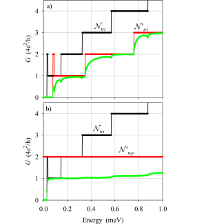
Figure 2: Conductance of electrostatic single junctions (green) of trivial-trivial type (a), and trivial-topological type (b). Black and red data show the number of propagating modes (Chern number) to the left and right sides of the junction, labeled as ${\cal N}_{\it tri}$, ${\cal N}^{\prime}_{\it tri}$ (a) and ${\cal N}_{\it tri}$, ${\cal N}^{\prime}_{\it top}$ (b), respectively. Parameters: $L_{y}=600$ nm, $L^{\prime}_{y}=400$ nm, $|V_{a}|=20$ meV, $s=12$ nm.

The conductance of the trivial-trivial junction (green, Fig. 2a) saturates to ${\cal N}^{\prime}_{\it tri}$ as the energy is increased, with the modifications of a rounding of the ${\cal N}^{\prime}_{\it tri}$ steps and small conductance dips at the onset of the ${\cal N}_{\it tri}$ steps. These features are rather similar to the results of semiconductor wire junctions in 2DEGS, the smoothened conductance being due to wave function reflections at the junction interface for energies near the activation onset of propagating modes.

In sharp contrast, the conductance of the trivial-topological junction (green, Fig. 2b) displays a conspicuously different behavior. In this case the conductance does not saturate to ${\cal N}^{\prime}_{\it top}$, at least not with a fast convergence as in the upper pannel. Actually, $G$ settles to a value close to 1 (in units of $G_{0}=4e^{2}/h$), in a plateau-like behaviour, with deviations of the quantized value becoming visible only when ${\cal N}_{\it tri}>4$.

The conductance quench of Fig. 2b to a value $G\approx 4e^{2}/h$, even when the topological kink-antikink system could in principle conduct ${\cal N}^{\prime}_{\it top}=2$ propagating modes (per valley and spin), is a remarkable feature. It is indicating that the incident modes from the trivial-side are mostly reflected except for one mode which is transmitted. We know that the modes on the topological side (kink-antikink) are localized to the $y$ values near the kink or the antikink and they have a valley dependent chirality. That is, two $K$ modes can be transmitted in the lower ($y<0$) kink, while two $K^{\prime}$ modes can be transmitted in the upper ($y>0$) antikink. A priori, the modes on the left (trivial) side are expected to be nonchiral, mostly propagating along the bulk of the wire $-L_{y}/2<y<L_{y}/2$. The observation that one mode is transmitted to the right, however, is strongly suggesting that one particular mode of the trivial wire is also edge-like and chiral, so that it can effectively couple to the chiral modes on the right side.

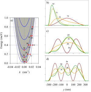
Figure 3: a) Energy bands of the trivial confinement wire with $L_{y}=600$ nm, $|V_{a}|=20$ meV, $s=12$ nm. The shaded region corresponds to the existence of real-$q$ modes, $k<k_{c}$ with $k_{c}$ the critical value given in Eq. (15). b,c,d) Probability densities for the $k$ values of the successive bands indicated with red dots in panel a).

The emergence of an edge chiral mode in an electrostatic BLG wire of trivial confinement is a surprising result, more so in absence of magnetic field such as our case. It is the main finding of our work. A valley-momentum-locked edge mode does not necessarily require a topological confinement with two nearby electrodes of opposite signs, as in the right side of Fig. 1b, but the simpler trivial electrode distribution in the left side of Fig. 1b or in Fig. 1a is also enough to sustain such a mode at the border between biased and unbiased BLG regions. This rather counterintuitive result is further discussed in the remaining of this Section and in Secs. III.2 and III.3.

Next, we validate our above interpretation by analysing the physical character of the modes of a trivial wire with numerical and analytical results. Figure 3 shows the band structure of a trivial 600-nm-wide wire and the spatial distributions of probablity densities for a few selected states along the lower energy branches. It only displays results for positive energy states since the negative-energy ones are mirror symmetric by energy and $y$ inversion, $E\to-E$ and $y\to-y$. Notice also that, while the energy branches are valley degenerate, the shown spatial distributions correspond to valley $K$. The corresponding distributions for $K^{\prime}$ are again given by $y$ inversion.

The results of Fig. 3 prove that the lowest branch of a trivial wire indeed becomes edge and chiral as the wave number $k\equiv p_{x}/\hbar$ is increased along the branch. Those results have been obtained numerically but is also possible to perform an analytical analysis.

III.2 Analytics

Assuming wave numbers $k$ and $q$ along $x$ and $y$, respectively, and a constant $V_{a}$ in Eq. (1) the eigenmode equation becomes an algebraic $4\times 4$ matrix problem for each valley, i.e., replacing $\tau_{z}\to s_{\tau}$ with $s_{\tau}=\pm 1$ for valley $K\,(K^{\prime})$.

In the purely homogenous case we can assume a spinorial wave function ($\sigma,\lambda=1,2$)

$$\Psi\equiv\Phi_{\sigma\lambda}\,e^{i(kx+qy)}\;,$$ (9)

with a 4-component spinor of constants $\Phi_{\sigma\lambda}$ for each $k$ and $q$. These constants are determined from the eigenvalue problem $H\Psi=E\Psi$ with the Hamiltonian of Eq. (1). We rewrite the eigenvalue problem as

$$\sigma_{y}H\Psi=E\sigma_{y}\Psi\;,$$ (10)

and with the $\Psi$ of Eq. (9) it can be recast as

$$\frac{1}{\hbar v_{F}}\left[\rule{0.0pt}{14.22636pt}E\,\sigma_{y}+is_{\tau}\,\hbar v_{F}\,k\,\sigma_{z}\right. + \frac{t}{2}\left(i\,\lambda_{x}\sigma_{z}-\lambda_{y}\right)$$ (11)

$$- \left.V_{a}\,\sigma_{y}\lambda_{z}\rule{0.0pt}{14.22636pt}\right]\Phi=q\,\Phi\;.$$

Equation (11) is a $4\times 4$ eigenvalue problem, ${\mathcal{M}}\,\Phi=q\,\Phi$, determining the transverse wave numbers $q$ for a given $E$ and $k$ from

$$\det\left({\mathcal{M}}-q\,\mathbf{1}\right)=0\;.$$ (12)

Straightforward algebra yields

$$q=\pm\frac{1}{\hbar v_{F}}\left[\rule{0.0pt}{11.38092pt}\right. - \hbar^{2}\,v_{F}^{2}\,k^{2}+V_{a}^{2}+E^{2}$$ (13)

$$\pm \sqrt{4V_{a}^{2}E^{2}+t^{2}(E^{2}-V_{a}^{2})}\,\left.\rule{0.0pt}{11.38092pt}\right]^{1/2}\;.$$

Equation (13) yields four $q$ roots whose character as purely real or complex numbers determine whether states having propagating or evanescent character along $y$ can emerge. If, for given $E$ and $k$, Eq. (13) has no real $q$, it necessarily implies that only transverse decaying states can emerge for those $E$ and $k$ values. In a large $V_{a}$, either positive or negative, all $q$’s are complex for reasonable $E$ and $k$ values, and thus states must necessarily decay. This is not surprising, since a large $V_{a}$ causes the decay in the sides of a trivial wire (Fig. 1a), and also the decay in the two directions when $y$ departs from the kink and antikink positions (Fig. 1b). Notice that a negative $V_{a}$ causes a similar decay of a positive $V_{a}$, a usual property of relativistic-like Dirac systems.

A surprising behavior for unbiased ($V_{a}=0$) BLG is that Eq. (13) still predicts a range of $E$ and $k$ values such that all $q$’s are complex. Naively, one could expect that unbiased BLG, being gapless, would only sustain bulk propagating states for any $k$. However, Eq. (13) for $V_{a}=0$ reads

$$q=\pm\frac{1}{\hbar v_{F}}\sqrt{-\hbar^{2}v_{F}^{2}\,k^{2}+|E|\left(\,|E|\pm t\,\right)}\;,$$ (14)

and, since $|E|<t$, it is then clear from Eq. (14) that all $q$’s are purely imaginary for $k>k_{c}$ where $k_{c}$ is the critical value

$$k_{c}=\frac{1}{\hbar v_{F}}\,\sqrt{|E|\,\left(\,|E|+t\,\right)}\;.$$ (15)

The shaded area in Fig. 3a corresponds to $k<k_{c}$, where real $q$’s exist. Notice that the lowest branch of Fig. 3a is then in the region of transverse decaying states, except for $k$ close to zero where the band presents a small maximum. This confirms the emerging edge chiral character of the lowest branch as $k$ is increased seen in Fig. 3b, as well as the bulk character of the states in Figs. 3cd.

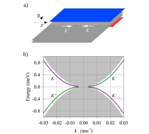
Figure 4: a) Sketch of a semi infinite interface between unbiased and biased BLG. The arrows indicate the propagation of the edge chiral mode for $K$ and $K^{\prime}$ valleys along the interface shown with a dotted line. b) Energy dispersion of the edge chiral modes. The shading corresponds to the continuum of states for $k<k_{c}$ of Eq. (15). Parameters: $|V_{a}|=20$ meV, $s=12$ nm.

III.3 Semi infinite unbiased-biased interface

Having identified an edge chiral mode in a trivial wire from the conductance of a trivial-topological junction, a natural question to address next is whether this mode is also present or not in a semi infinite interface between unbiased and biased BLG (Fig. 4a). We have then calculated the transverse localized states by numerically imposing zero boundary condition for $y\to\pm\infty$ with the electrode configuration sketched in Fig. 4a. Indeed, for $k>k_{c}$ a localized state is found with the energy dispersion of Fig. 4b for $K$ (magenta) and $K^{\prime}$ (green) valleys.

Figure 4 highlights the opposite chiralities of the $K$ and $K^{\prime}$ edge modes propagating along the dotted line interface. The modes are characterized by their opposite slopes for $K$ and $K^{\prime}$, indicating their valley-momentum locking, similarly to the topological modes of a kink.Martin et al. (2008) However, clear differences with the kink modes are: a) only one mode per valley is present in Fig. 4 while there are two kink modes per valley; b) kink modes lie in an energy-gapped region of the spectrum, while the present edge chiral modes co-exist with bulk modes of the shaded area of Fig. 4 lying at the same energy. In fact, the edge chiral branches even merge with the continuum for $k$ close to zero. Appendix A provides further analysis of the edge chiral modes using quasi-analytic complementary approaches and also investigating their robustness against the diffusivity $s$ and the value of the asymmetry potential $V_{a}$.

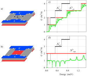
Figure 5: a,b) Sketches of the double junction setups similar to Fig. 1. The length of the central part is $L_{x}=1\;\mu{\rm m}$. c,d) Results of the double junctions shown on the corresponding left panels. Black line is indicating the number of modes in trivial left and right leads, while red is the number of modes in the center, which can be either trivial (a,c) or topological (b,d). Rest of parameters as in Fig. 2.

III.4 Wire double junctions

As a final item of this work, we address the study of the double junctions with trivial leads and a scattering center which is either also trivial or topological. Sketches of the two types of double junctions can be seen in Fig. 5ab. In these geometries a new parameter appears as compared to the preceding single junctions, the length $L_{x}$ of the central section. The double junction with a trivial center (Fig. 5c) displays similar results to the trivial-trivial single junction (Fig. 2a). The conductance saturates to ${\cal N}^{\prime}_{\it tri}$ as the energy increases. The rounded steps are now transformed into short oscillations. They are caused by interferences of Fabry-Pérot type due to multiple reflections between the first and the second interfaces of the junction. The oscillation amplitude is larger near the activation thresholds of transmitted modes, ${\cal N^{\prime}}_{\it tri}\to{\cal N^{\prime}}_{\it tri}+1$, and it smoothly decays for increasing energy until the next activation threshold is reached. The thresholds for incident modes, ${\cal N}_{\it tri}\to{\cal N}_{\it tri}+1$, also leave a trace on the conductance curve and, in particular, a rather flat conductance is seen for $({\cal N}_{\it tri},{\cal N^{\prime}}_{\it tri})=(4,2)$ and $(5,3)$. The Fabry-Pérot interferences would be strongly enhanced in presence of barriers at the junction interfaces (dotted lines in Fig. 5a) but this would require using additional electrodes.

The conductance of the double junction with a topological center (Fig. 5d) shows outstanding features. The quenching to $G\approx 4e^{2}/h$ due to the transmission of a single edge chiral mode of the trivial wire is again observed, as in Fig. 2b. However, a remarkable sequence of dips and peaks is now found in the double junction. These features are an evidence of the spectrum of topological eigenstates forming closed loops around the central region of the double junction. The energies of those topological loops can be well described by a Bohr-Sommerfeld quantization rule,Benchtaber et al. (2021b) requiring an integer number of wave lengths fit into the loop perimeter. The dips or peaks are then consequences of Fano resonances due to the coupling of localized states, the closed loops, with the scattering states. The effective coupling varies with energy and transforms the resonances from dips at low energy into peaks at higher energy in Fig. 5d.

Fano resonance profiles are characterized asFano (1961); Nöckel and Stone (1994); Sánchez and Serra (2006)

$$G\approx\frac{|\epsilon+q|^{2}}{\epsilon^{2}+1}\;,$$ (16)

where $q$ is the Fano parameter and the energy dependence is contained in $\epsilon\equiv(E-E_{R})/\Gamma$, with $E_{R}$ and $\Gamma$ the resonance energy and width. Different values of the Fano parameter $q$ yield varying resonance profiles, from symmetric dips ($q\to 0$) to intermediate asymmetric profiles (finite $q$’s) and symmetric peaks (large $q$’s). Figure 5 is indicating a fast evolution of the Fano parameter with energy, asymmetry profile being observed only around 0.85 meV for that specific set of parameters. A detailed analytical modeling of the coupling between the topological closed loops and the scattering states requires a fine tuning of the coupling intensities and is out of the scope of the present work.

IV Conclusions

Junctions of electrostatically confined BLG wires show outstanding transport features feasible to be detected. A trivial-topological junction is characterized by a conductance quench with respect to a trivial-trivial junction. A single mode of edge chiral character, per valley and spin, is transmitted from the trivial to the topological side causing a near quantization $G\approx 4e^{2}/h$ when the number of incident modes is low (${\cal N}_{\it tri}<4)$. With larger values of ${\cal N}_{\it tri}$ the conductance deviation from the quantized value becomes increasingly visible.

The edge chiral character of the lowest mode of a trivial BLG wire is surprising, more so in the absence of any magnetic field. Such mode is also present at a semi infinite interface between unbiased and biased BLG planes. It is characterized by a locking between valley and momentum and there is an analytical critical value of momentum $k_{c}$ for the presence of such mode when $k>k_{c}$, which is otherwise damped in the continuum of bulk states.

Double junctions of electrostatic BLG wires with trivial leads and a topological center show conspicuous Fano resonances, dips or peaks in the conductance. They are due to an energy-dependent coupling of the closed loop around the topological center and the scattering states. Altogether, the above features may help to place hybrid trivial-topological BLG graphene wires with electrostatic confinement as a useful and controllable platform for graphene electronics.

Appendix A The edge chiral mode

In this appendix we analyze further the existence of an edge chiral mode at the boundary between unbiased ($V_{a}=0$) and biased ($V_{a}\neq 0$) BLG as sketched in Fig. 4a. Specifically, we obtain such mode in two complementary approaches. First we use a $y$-grid diagonalization as in Fig. 4b to investigate the dependence of the mode dispersion on the asymmetry potential diffusivity $s$ and on its saturating value $V_{a}$. Second, we use a quasi-analytic method valid for the sharp interface, imposing the matching of the properly decaying solutions on the two sides of the interface. The two approaches are in excellent agreement and thus support the physical existence of the edge chiral mode.

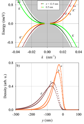
Figure 6: a) Energy dispersion of the $K$ and $K^{\prime}$ edge chiral mode for the semi infinite interface (Fig. 4a) and for two different values of the diffusivity parameter $s$. We have assumed $V_{a}=20$ meV and the shaded region corresponds to $k<k_{c}$. b) Spatial distribution of the probability densities for the indicated states of panel a). The solid lines in panels a) and b) are the results of the quasi-analytic model for a sharp interface and they show an excellent agreement with the $s=0.5$ nm smooth potential data.

Figure 6 addresses the dependence on the smoothness $s$, showing that the sharper the asymmetry potential the larger the separation of the mode branch from the continuum indicated in gray. The lower panel Fig. 6b shows that the probability densities with a larger $s$ extend farther from the interface than the densities for smaller $s$, as one could intuitively expect. We have also obtained (not shown in the figure) that the probability distributions are unchanged when reversing the momentum ($k\leftrightarrow-k$) for a given valley, or reversing the valley ($K\leftrightarrow K^{\prime}$) for a given momentum.

In case of a sharp transition interface $s=0$ we have solved the matching condition at the interface considering exponentially decaying solutions towards both sides. The $q$ wave numbers and $\Phi$ wave functions are determined from Eq. (13) and Eq. (11), respectively. The matching approach does not use any grid discretization of the $y$ coordinate and only requires the calculation of $4\times 4$ matrices, as determined by the number of $q$ modes. The results are in excellent agreement with the grid result for small diffusivity, as shown by the solid lines of Fig. 6a, thus confirming the physical character of the edge chiral mode. We also stress that the two methods prove that there is only one branch for $K$ and one branch for $K^{\prime}$, differently to the result for kink states yielding two branches per valley.Martin et al. (2008); Zarenia et al. (2011) Notice, however, that the present chiral edge branches are not topologically protected from the continuum of bulk states (gray) by an energy gap, as occurs for the kink states.

Finally, the dependence on $V_{a}$ is analyzed in Fig. 7. The energy dispersion $E(k)$ becomes flatter with increasing $V_{a}$ (Fig. 7a) while the density distribution becomes narrower (Fig. 7b), corresponding to a more localized state at the interface. Nevertheless, the mode features are qualitatively preserved even with large changes in $V_{a}$.

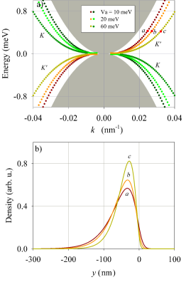
Figure 7: Same as Fig. 6 for different values of the asymmetry potential $V_{a}$. We assumed a sharp interface $s=0.5$ nm.

References

- McCann and Koshino (2013) Edward McCann and Mikito Koshino, “The electronic properties of bilayer graphene,” Reports on Progress in Physics 76, 056503 (2013).
- Zhang et al. (2013) Fan Zhang, Allan H. MacDonald, and Eugene J. Mele, “Valley chern numbers and boundary modes in gapped bilayer graphene,” Proceedings of the National Academy of Sciences 110, 10546–10551 (2013).
- Rozhkov et al. (2016) A.V. Rozhkov, A.O. Sboychakov, A.L. Rakhmanov, and Franco Nori, “Electronic properties of graphene-based bilayer systems,” Physics Reports 648, 1–104 (2016), electronic properties of graphene-based bilayer systems.
- Overweg et al. (2018) Hiske Overweg, Angelika Knothe, Thomas Fabian, Lukas Linhart, Peter Rickhaus, Lucien Wernli, Kenji Watanabe, Takashi Taniguchi, David Sánchez, Joachim Burgdörfer, Florian Libisch, Vladimir I. Fal’ko, Klaus Ensslin, and Thomas Ihn, “Topologically nontrivial valley states in bilayer graphene quantum point contacts,” Phys. Rev. Lett. 121, 257702 (2018).
- Kraft et al. (2018) R. Kraft, I. V. Krainov, V. Gall, A. P. Dmitriev, R. Krupke, I. V. Gornyi, and R. Danneau, “Valley subband splitting in bilayer graphene quantum point contacts,” Phys. Rev. Lett. 121, 257703 (2018).
- Eich et al. (2018) Marius Eich, F. Herman, Riccardo Pisoni, Hiske Overweg, Annika Kurzmann, Yongjin Lee, Peter Rickhaus, Kenji Watanabe, Takashi Taniguchi, Manfred Sigrist, Thomas Ihn, and Klaus Ensslin, “Spin and valley states in gate-defined bilayer graphene quantum dots,” Phys. Rev. X 8, 031023 (2018).
- Kurzmann et al. (2019) Annika Kurzmann, Hiske Overweg, Marius Eich, Alessia Pally, Peter Rickhaus, Riccardo Pisoni, Yongjin Lee, Kenji Watanabe, Takashi Taniguchi, Thomas Ihn, and Klaus Ensslin, “Charge detection in gate-defined bilayer graphene quantum dots,” Nano Letters 19, 5216–5221 (2019).
- Banszerus et al. (2020) L. Banszerus, A. Rothstein, T. Fabian, S. Möller, E. Icking, S. Trellenkamp, F. Lentz, D. Neumaier, K. Watanabe, T. Taniguchi, F. Libisch, C. Volk, and C. Stampfer, “Electron hole crossover in gate-controlled bilayer graphene quantum dots,” Nano Letters 20, 7709–7715 (2020).
- Banszerus et al. (2021) L. Banszerus, K. Hecker, E. Icking, S. Trellenkamp, F. Lentz, D. Neumaier, K. Watanabe, T. Taniguchi, C. Volk, and C. Stampfer, “Pulsed-gate spectroscopy of single-electron spin states in bilayer graphene quantum dots,” Phys. Rev. B 103, L081404 (2021).
- Meng et al. (2012) Lan Meng, Zhao-Dong Chu, Yanfeng Zhang, Ji-Yong Yang, Rui-Fen Dou, Jia-Cai Nie, and Lin He, “Enhanced intervalley scattering of twisted bilayer graphene by periodic stacked atoms,” Phys. Rev. B 85, 235453 (2012).
- Clericò et al. (2019) V. Clericò, J. A. Delgado-Notario, M. Saiz-Bretín, A. V. Malyshev, Y. M. Meziani, P. Hidalgo, B. Méndez, M. Amado, F. Domínguez-Adame, and E. Diez, “Quantum nanoconstrictions fabricated by cryo-etching in encapsulated graphene,” Sci. Rep. 9, 13572 (2019).
- Pereira et al. (2007) J. M. Pereira, P. Vasilopoulos, and F. M. Peeters, “Tunable quantum dots in bilayer graphene,” Nano Letters 7, 946–949 (2007).
- Recher et al. (2009) Patrik Recher, Johan Nilsson, Guido Burkard, and Björn Trauzettel, “Bound states and magnetic field induced valley splitting in gate-tunable graphene quantum dots,” Phys. Rev. B 79, 085407 (2009).
- Zarenia et al. (2009) M. Zarenia, J. M. Pereira, F. M. Peeters, and G. A. Farias, “Electrostatically confined quantum rings in bilayer graphene,” Nano Letters 9, 4088–4092 (2009).
- Pereira et al. (2009) J. M. Pereira, F. M. Peeters, P. Vasilopoulos, R. N. Costa Filho, and G. A. Farias, “Landau levels in graphene bilayer quantum dots,” Phys. Rev. B 79, 195403 (2009).
- Zarenia et al. (2010a) M. Zarenia, J. M. Pereira, A. Chaves, F. M. Peeters, and G. A. Farias, “Simplified model for the energy levels of quantum rings in single layer and bilayer graphene,” Phys. Rev. B 81, 045431 (2010a).
- Zarenia et al. (2010b) M. Zarenia, J. M. Pereira, A. Chaves, F. M. Peeters, and G. A. Farias, “Erratum: Simplified model for the energy levels of quantum rings in single layer and bilayer graphene [Phys. Rev. B 81, 045431 (2010)],” Phys. Rev. B 82, 119906(E) (2010b).
- da Costa et al. (2014) D.R. da Costa, M. Zarenia, Andrey Chaves, G.A. Farias, and F.M. Peeters, “Analytical study of the energy levels in bilayer graphene quantum dots,” Carbon 78, 392–400 (2014).
- Martin et al. (2008) Ivar Martin, Ya. M. Blanter, and A. F. Morpurgo, “Topological confinement in bilayer graphene,” Phys. Rev. Lett. 100, 036804 (2008).
- Zarenia et al. (2011) M. Zarenia, J. M. Pereira, G. A. Farias, and F. M. Peeters, “Chiral states in bilayer graphene: Magnetic field dependence and gap opening,” Phys. Rev. B 84, 125451 (2011).
- Xavier et al. (2010) L. J. P. Xavier, J. M. Pereira, Andrey Chaves, G. A. Farias, and F. M. Peeters, “Topological confinement in graphene bilayer quantum rings,” Applied Physics Letters 96, 212108 (2010).
- Benchtaber et al. (2021a) Nassima Benchtaber, David Sánchez, and Llorenç Serra, “Scattering of topological kink-antikink states in bilayer graphene structures,” Phys. Rev. B 104, 155303 (2021a).
- Benchtaber et al. (2021b) Nassima Benchtaber, David Sánchez, and Llorenç Serra, “Geometry effects in topologically confined bilayer graphene loops,” New Journal of Physics 24, 013001 (2021b).
- Ju et al. (2015) Long Ju, Zhiwen Shi, Nityan Nair, Yinchuan Lv, Chenhao Jin, Jairo Velasco, Claudia Ojeda-Aristizabal, Hans A. Bechtel, Michael C. Martin, Alex Zettl, James Analytis, and Feng Wang, “Topological valley transport at bilayer graphene domain walls,” Nature 520, 650–655 (2015).
- Sui et al. (2015) Mengqiao Sui, Guorui Chen, Liguo Ma, Wen-Yu Shan, Dai Tian, Kenji Watanabe, Takashi Taniguchi, Xiaofeng Jin, Wang Yao, Di Xiao, and Yuanbo Zhang, “Gate-tunable topological valley transport in bilayer graphene,” Nature Physics 11, 1027–1031 (2015).
- Li et al. (2016) Jing Li, Ke Wang, Kenton J. McFaul, Zachary Zern, Yafei Ren, Kenji Watanabe, Takashi Taniguchi, Zhenhua Qiao, and Jun Zhu, “Gate-controlled topological conducting channels in bilayer graphene,” Nature Nanotechnology 11, 1060–1065 (2016).
- Chen et al. (2020) H. Chen, P. Zhou, J. Liu, J. Qiao, B. Oezyilmaz, and J. Martin, “Gate controlled valley polarizer in bilayer graphene,” Nature Communications 11, 1202 (2020).
- Snyman and Beenakker (2007) I. Snyman and C. W. J. Beenakker, “Ballistic transmission through a graphene bilayer,” Phys. Rev. B 75, 045322 (2007).
- González et al. (2010) J. W. González, H. Santos, M. Pacheco, L. Chico, and L. Brey, “Electronic transport through bilayer graphene flakes,” Phys. Rev. B 81, 195406 (2010).
- Osca and Serra (2019) Javier Osca and Llorenç Serra, “Complex band-structure analysis and topological physics of Majorana nanowires,” Eur. Phys. J. B 92, 101 (2019).
- Susskind (1977) Leonard Susskind, “Lattice fermions,” Phys. Rev. D 16, 3031–3039 (1977).
- Nielsen and Ninomiya (1981) H.B. Nielsen and M. Ninomiya, “Absence of neutrinos on a lattice: (I). Proof by homotopy theory,” Nuclear Physics B 185, 20–40 (1981).
- Hernández and Lewenkopf (2012) Alexis R. Hernández and Caio H. Lewenkopf, “Finite-difference method for transport of two-dimensional massless Dirac fermions in a ribbon geometry,” Phys. Rev. B 86, 155439 (2012).
- Fano (1961) U. Fano, “Effects of configuration interaction on intensities and phase shifts,” Phys. Rev. 124, 1866–1878 (1961).
- Nöckel and Stone (1994) Jens U. Nöckel and A. D. Stone, “Resonance line shapes in quasi-one-dimensional scattering,” Phys. Rev. B 50, 17415–17432 (1994).
- Sánchez and Serra (2006) David Sánchez and Llorenç Serra, “Fano-Rashba effect in a quantum wire,” Phys. Rev. B 74, 153313 (2006).