A Software Tool for ”Gluing” Distributions

Abstract

When performing Monte-Carlo simulations, distributions are sometimes determined only for sub-intervals of the desired total range. In such cases, a frequent problem is to connect, or glue, individual distributions to obtain the final result. Most prominent examples, where this is usually necessary, are certain large-deviation simulation techniques. However, there are multiple approaches to do this, depending on the data and individual requirements. Here, a software tool is presented, containing multiple algorithms, to aid with this task. An introduction to the available methods is presented together with a short tutorial using exemplary data.

I Introduction

In large-deviation Monte-Carlo simulations Hartmann (2002, 2014); Börjes et al. (2019); Werner and Hartmann (2021) usually multiple runs are performed that are targeting different ranges for the quantity of interest to obtain its distribution in the desired regime of rare events. One important part of the data post-processing is to connect the individual histograms to one final distribution. The software tool that is showcased here was originally developed with this specific use case in mind, but also extends beyond. It can be useful for any variant of Monte-Carlo simulation, even without a relation to large-deviations, and experimental data alike.

In the following, it is first explained how to obtain and run the tool. Subsequently, there is a description of the implemented algorithms. Finally, a tutorial is given that demonstrates the core functionality using exemplary data.

I.1 How to obtain the tool?

The tool is available through the repository https://gitlab.uni-oldenburg.de/ag-computerphysik/distribution-gluer , from where it can either be cloned via git or directly downloaded by a web-browser. It comes in the form of a python3-script.

I.2 How to run the tool?

To run the script, a recent version of Anaconda https://www.anaconda.com/products/individual is recommended. Otherwise, the following libraries must be installed in a local python3 environment: numpy, gmpy2, matplotlib and scipy. As a starting point, typing

ΨΨ  python3 distribution_gluer.py --help
ΨΨ

into a command line will display an overview of all options. The displayed help-output also serves as the main reference for the program.

II Gluing Algorithms

The tool can handle raw data, which is naively just a file containing one column of real valued numbers, or data that is already processed into a histogram. For raw data, the tool can determine the corresponding histograms by itself. In any case, as a result of numerical simulations Hartmann (2015); Newman and Barkema (1999) or obtained otherwise, let there be $N$ histograms $H_{\Theta_{i}}(x)$ with $i=1,\dots,N$ for an arbitrary bin center value $x$. The corresponding errors are denoted by $\sigma_{\Theta_{i}}(x)$. The value $\Theta_{i}$ is a simulation parameter on which the histograms depend, usually the temperature or a temperature like parameter. For example in large deviation simulations Hartmann (2002, 2014); Börjes et al. (2019); Werner and Hartmann (2021), these are typically used to control the extend by which the simulation is steered towards rare events. Here, $\Theta_{i}$ is referred to as a pseudo-temperature, even though it can be an actual temperatures as well. This dependence can, but does not have to, result in a bias that needs to be accounted for prior to connecting the distributions by multiplying with a factor $f(\Theta,x)$:

$$H_{i}(x) =H_{\Theta_{i}}(x)f(\Theta_{i},x)$$ (1)

$$\sigma_{i}(x) =\sigma_{\Theta_{i}}(x)f(\Theta_{i},x).$$ (2)

This factor could be just $f(\Theta,x)=1$ in case all pseudo-temperatures are the same $\Theta_{i}=\Theta$, but the histograms were determined over different intervals (e.g. as it is the case for Wang-Landau sampling Wang and Landau (2001); Vogel et al. (2014)). Or when the overall quantity of interest is the energy-state-density of a physical system following the Boltzmann-distribution, the factor would be $f(\Theta,x)=\exp{(x/\Theta)}$.

At this point in time, the tool offers two ways, namely the Least-Squares (LSQRS) and the Ferrenberg-Swendsen (FS) Ferrenberg and Swendsen (1989) method, to connect histograms/distributions, which are described briefly in the following.

II.1 Least-Squares-Method

The LSQRS method tries to minimize the squared difference

$$\Delta(g_{i},g_{j})=\sum_{x\in\mathcal{M}_{i,j}}\frac{(g_{i}H_{i}(x)-g_{j}H_{j}(x))^{2}}{\sigma_{i}^{2}(x)+\sigma_{j}^{2}(x)}$$ (3)

between two histograms $i,j=1,\dots,N$ and $i\neq j$, where $\mathcal{M}_{i,j}$ is the set of bins $x$ for which both histograms have a non-zero count, i.e. $H_{i}(x)\neq 0\wedge H_{j}(x)\neq 0$. Additionally, the weights $g_{i},g_{j}\neq 0$ have to fulfill the side condition of a normalized total distribution. There is an analytical solution to eq. (3) (see appendix A) resulting in a weighting factor $g_{i}$ for each histogram. Subsequently, these are used to determine the final probability density and uncertainty

$$p(x) =\frac{\sum_{i=1}^{N}\frac{g_{i}H_{i}(x)}{(g_{i}\sigma_{i}(x))^{2}}}{\sum_{j=1}^{N}\frac{1}{(g_{j}\sigma_{j}(x))^{2}}}$$ (4)

$$\sigma_{p}(x) =\frac{1}{\sqrt{\sum_{i=1}^{N}\frac{1}{(g_{i}\sigma_{i}(x))^{2}}}}.$$ (5)

II.2 Ferrenberg-Swendsen-Method

The FS method assumes a particular bias of $f(\Theta_{i},x)=\exp{(x/\Theta_{i})}$ on the histograms $H_{\Theta_{i}}(x)$, which is in contrast to the LSQRS method that works with any form of bias. According to Ferrenberg and Swendsen (1989), the final distribution is obtained by solving the equations

$$p(x) =\frac{\sum_{i=1}^{N}H_{\Theta_{i}}(x)}{\sum_{j=1}^{N}e^{-\frac{x}{\Theta_{j}}+h_{j}}\sum_{\tilde{x}}H_{\Theta_{j}}(\tilde{x})}$$ (6)

$$e^{-h_{i}} =\sum_{x}p(x)e^{-\frac{x}{\Theta_{i}}}$$ (7)

numerically for $h_{i}$ ($i=1,\dots,N$) with an iterative procedure. The uncertainty on $p(x)$ is given by Ferrenberg and Swendsen (1989)

$$\sigma_{p}(x)=\frac{p(x)}{\sqrt{\left(\sum_{i=1}^{N}H_{\Theta_{i}}(x)\right)}}.$$ (8)

III Tutorial

This tutorial assumes basic knowledge in using a command line interpreter/shell (e.g. bash). The tool comes with example data contained in the archive file example_data.zip, which should be unpacked before trying the following commands. The data can either be in raw form or already be histogramed. For reference on the specific file formatting, see the -f option of the help-output. In order to process raw data the -c option has to be selected, which will let the tool create the histograms by itself (see https://numpy.org/doc/stable/reference/generated/numpy.histogram˙bin˙edges.html for technical reference; the bins=’auto’ argument is used). For convenience also the -P option is set in the following commands, yielding a plot of the result. The displayed figure shows in the bottom plot the original histograms and in the top one, depending on the gluing method, for LSQRS the individual reweighted histograms and for FS the final distribution. The legend indicates the corresponding pseudo-temperatures when provided. The final distribution is written to the output file output.txt as specified by the -o option. If no gluing method is set, the tool defaults to LSQRS.

III.1 Raw unbiased data

In order to combine all files in the directory raw_unbiased_data into one distribution, the command

ΨΨ  python3 distribution_gluer.py -f \
ΨΨ  example_data/raw_unbiased_data/* -c -P \
ΨΨ  -o output.txt
ΨΨ

can be used.

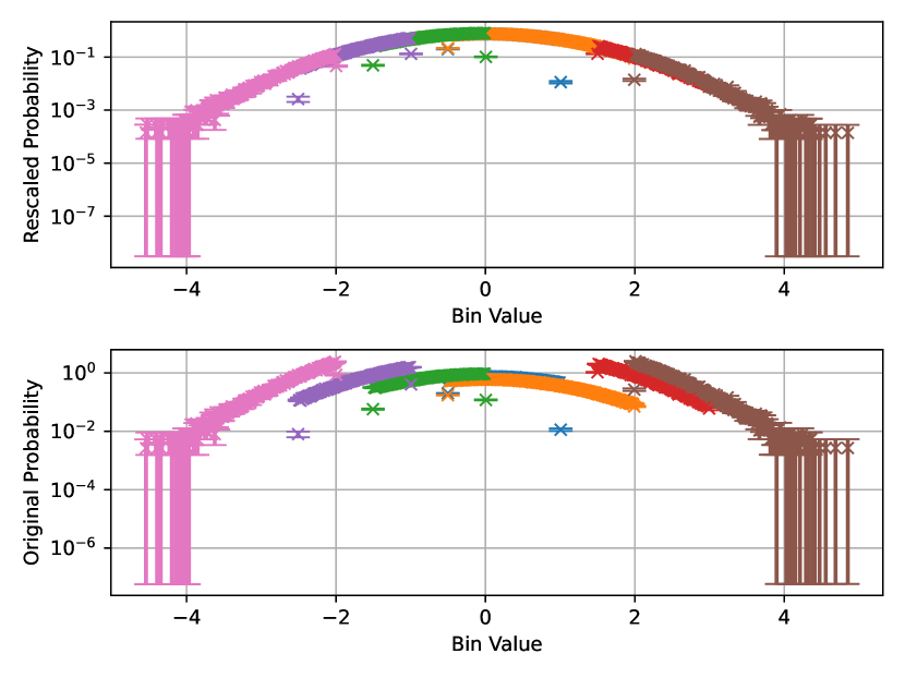
Figure 1: Program output plot example for raw unbiased data. Top: Glued/Rescaled distributions using the LSQRS method. Bottom: Original histograms determined by the gluing tool.

An example of how the displayed plot might look like is given in Fig. 1.
To improve the result, separate binning intervals can be specified using the -b BINNING_SEPERATOR1 BINNING_SEPERATOR2 … option. Each of the separator variables marks the interval edges for which the internal binning algorithm is run independently. This can be helpful, when there are regions with fewer data points:

ΨΨ  python3 distribution_gluer.py -f \
ΨΨ  example_data/raw_unbiased_data/* -c -P \
ΨΨ  -o output.txt -b -3 3
ΨΨ

It is also possible to completely ignore any standard deviation on the histogram bins with the -i option:

ΨΨΨΨ  python3 distribution_gluer.py -f \
ΨΨΨΨ  example_data/raw_unbiased_data/* -c -P \
ΨΨΨΨ  -o output.txt -b -3 3 -i
ΨΨ

Sometimes it is useful to cut off outlying values from the individual histograms, before applying the LSQRS-method. The -s STD_MULTIPLE option will discard any bins that are more than the specified multiple of the standard deviation away from the mean:

ΨΨ  python3 distribution_gluer.py -f \
ΨΨ  example_data/raw_unbiased_data/* -c -P \
ΨΨ  -o output.txt -b -3 3 -s 3
ΨΨ

III.2 Histogrammed unbiased data

Like with the case of raw unbiased data, it is possible to combine data that is already processed into histograms:

ΨΨ  python3 distribution_gluer.py -f \
ΨΨ  example_data/histogrammed_unbiased_data/* \
ΨΨ  -P -o output.txt
ΨΨ

III.3 Raw biased data

For biased data, pseudo temperatures have to be provided (option -p PSEUDO1 PSEUDO2 …), where a bias of the form $f(\Theta_{i},x)=\exp{(x/\Theta_{i})}$ is assumed. The FS method is selected via the -g FS option. In the following command, also a file containing specific bin edges (option -B BINNING_FILE) is provided:

ΨΨ  PSEUDO={-10.0,10.0,-2.0,2.0,-4.0,4.0,\
ΨΨ  Ψ-6.0,6.0,-8.0,8.0,inf};\
ΨΨ  python3 distribution_gluer.py -f \
ΨΨ  $(eval echo example_data/raw_biased_data\
ΨΨ  /pseudo_$PSEUDO.dat) \
ΨΨ  -p $(eval echo $PSEUDO) \
ΨΨ  -B example_data/raw_biased_data\
ΨΨ  /bin_edges.txt -c -P -o output.txt -g FS
ΨΨ

III.4 Histogrammed biased data

Again, it is also possible to work with histograms of biased data directly:

ΨΨ  PSEUDO={-10.0,10.0,-2.0,2.0,-4.0,4.0\
ΨΨ  ,-6.0,6.0,-8.0,8.0,inf};\
ΨΨ  python3 distribution_gluer.py -f \
ΨΨ  $(eval echo example_data\
ΨΨ  /histogrammed_biased_data\
ΨΨ  /pseudo_$PSEUDO.dat) \
ΨΨ  -p $(eval echo $PSEUDO) -P \
ΨΨ  -o output.txt -g FS
ΨΨ

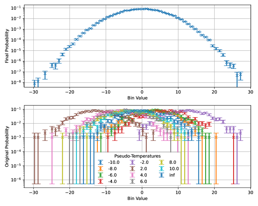
Figure 2: Program output plot example for biased histogrammed data. Top: Glued final distribution using the FS method. Bottom: Original biased histograms at different pseudo-temperatures $\Theta_{i}$ provided to the gluing tool.

An example of the program output plot for this command is displayed in Fig. 2.
Biased histograms can also be treated with the default LSQRS method using:

ΨΨ  PSEUDO={-10.0,10.0,-2.0,2.0,-4.0,4.0\
ΨΨ  Ψ,-6.0,6.0,-8.0,8.0,inf}; \
ΨΨ  python3 distribution_gluer.py -f \
ΨΨ  $(eval echo example_data\
ΨΨ  /histogrammed_biased_data\
ΨΨ  /pseudo_$PSEUDO.dat) \
ΨΨ  -p $(eval echo $PSEUDO) -P -o output.txt
ΨΨ

IV Final Remarks

The tool is in continuous development and any comments and suggestions for improvement are very welcome. The author wishes to thank Alexander K. Hartmann for carefully reading the manuscript and testing the program.

Appendix A Analytical solution for LSQRS method weight factors

Rewriting eq. (3) with relative weights $g_{ij}:=g_{j}/g_{i}$ (relative weights have two indices and absolute weights one) yields

$$\tilde{\Delta}(g_{ij}):=\sum_{x\in\mathcal{M}_{i,j}}\frac{(H_{i}(x)-g_{ij}H_{j}(x))^{2}}{\sigma_{i}^{2}(x)+\sigma_{j}^{2}(x)}.$$ (9)

The minimal squared difference must satisfy the condition $\frac{\partial\tilde{\Delta}}{\partial g_{ij}}\overset{!}{=}0$, resulting in

$$g_{ij}=\frac{\sum_{x\in\mathcal{M}_{i,j}}\frac{H_{i}(x)H_{j}(x)}{\sigma_{i}^{2}(x)+\sigma_{j}^{2}(x)}}{\sum_{x^{\prime}\in\mathcal{M}_{i,j}}\frac{H^{2}_{j}(x^{\prime})}{\sigma_{i}^{2}(x^{\prime})+\sigma_{j}^{2}(x^{\prime})}}.$$ (10)

For relative weights between non-overlapping histograms (i.e. $\mathcal{M}=\emptyset$) eq. (10) is not applicable. However, these can be calculated in a chain like manner. When $g_{ij}$ and $g_{jk}$ with $i\neq j\neq k$ are known and the relative weight of interest $g_{ik}$ can not be calculated directly via eq. (10), it is still possible to use

$$g_{ik}=\frac{g_{k}}{g_{i}}=\frac{g_{j}}{g_{i}}\frac{g_{k}}{g_{j}}=g_{ij}g_{jk}.$$ (11)

By fixing one of the absolute weight factors (e.g. $g_{i}$) such that the total distribution is normalized, all other weights $g_{j}$ are determined by

$$g_{j}=g_{ij}g_{i}.$$ (12)

References

- Hartmann (2002) A. K. Hartmann, Phys. Rev. E 65, 056102 (2002).
- Hartmann (2014) A. K. Hartmann, Phys. Rev. E 89, 052103 (2014).
- Börjes et al. (2019) J. Börjes, H. Schawe, and A. K. Hartmann, Phys. Rev. E 99, 042104 (2019).
- Werner and Hartmann (2021) P. Werner and A. K. Hartmann, Phys. Rev. E 104, 034407 (2021).
- (5) https://gitlab.uni-oldenburg.de/ag-computerphysik/distribution-gluer, .
- (6) https://www.anaconda.com/products/individual, .
- Hartmann (2015) A. K. Hartmann, Big Practical Guide to Computer Simulations, 2nd ed. (WORLD SCIENTIFIC, 2015) https://www.worldscientific.com/doi/pdf/10.1142/9019 .
- Newman and Barkema (1999) M. E. J. Newman and G. T. Barkema, Monte Carlo methods in statistical physics (1999).
- Wang and Landau (2001) F. Wang and D. P. Landau, Phys. Rev. Lett. 86, 2050 (2001).
- Vogel et al. (2014) T. Vogel, Y. W. Li, T. Wüst, and D. P. Landau, Phys. Rev. E 90, 023302 (2014).
- Ferrenberg and Swendsen (1989) A. M. Ferrenberg and R. H. Swendsen, Phys. Rev. Lett. 63, 1195 (1989).
- (12) https://numpy.org/doc/stable/reference/generated/numpy.histogram_bin_edges.html, .