The Variable Projected Augmented Lagrangian Method

Abstract

Inference by means of mathematical modeling from a collection of observations remains a crucial tool for scientific discovery and is ubiquitous in application areas such as signal compression, imaging restoration, and supervised machine learning. The inference problems may be solved using variational formulations that provide theoretically proven methods and algorithms. With ever-increasing model complexities and growing data size, new specially designed methods are urgently needed to recover meaningful quantifies of interest. We consider the broad spectrum of linear inverse problems where the aim is to reconstruct quantities with a sparse representation on some vector space; often solved using the (generalized) least absolute shrinkage and selection operator (lasso). The associated optimization problems have received significant attention, in particular in the early 2000’s, because of their connection to compressed sensing and the reconstruction of solutions with favorable sparsity properties using augmented Lagrangians, alternating directions and splitting methods. We provide a new perspective on the underlying $\ell^{1}$ regularized inverse problem by exploring the generalized lasso problem through variable projection methods. We arrive at our proposed variable projected augmented Lagrangian (vpal) method. We analyze this method and provide an approach for automatic regularization parameter selection based on a degrees of freedom argument. Further, we provide numerical examples demonstrating the computational efficiency for various imaging problems.

65F10, 65F22, 65F20, 90C06

1 Introduction

Many scientific problems are modeled as

(1) $$\mathbf{b}=\mathbf{A}\mathbf{x}_{\rm true}+\text{\boldmath$\mathbf{\varepsilon}$},$$

where $\mathbf{x}_{\rm true}\in\mathbb{R}^{n}$ is a desired solution, $\mathbf{A}\in\mathbb{R}^{m\times n}$ denotes a forward process that includes a physical model and the mapping onto observations $\mathbf{b}\in\mathbb{R}^{m}$, and $\mathbf{\varepsilon}$ is, for simplicity, some unknown additive Gaussian noise $\text{\boldmath$\mathbf{\varepsilon}$}\sim\mathcal{N}({\bf 0},\sigma^{2}\mathbf{I}_{m})$. Given observations $\mathbf{b}$ and the forward process $\mathbf{A}$, in inverse problems we aim to obtain an approximate solution $\widehat{\mathbf{x}}$ to $\mathbf{x}_{\rm true}$ [40]. We assume the inverse problem is either ill-posed (i.e., a solution does not exist, is not unique, or does not depend continuously on the data [37]) or that we are given specific prior knowledge about the unknown $\mathbf{x}_{\rm true}$. Inverse problems arise in many different fields, such as medical imaging, geophysics, and signal processing to name a few [41, 48, 59].

Regularization is included to incorporate the prior knowledge and/or to stabilize the inversion process to obtain a meaningful approximation $\widehat{\mathbf{x}}$. Many types of regularization exist; here we focus on the variational regularization problem

(2) $$\widehat{\mathbf{x}}\in\operatorname*{arg\,min}_{\mathbf{x}}\ \tfrac{1}{2}\left\|\mathbf{A}\mathbf{x}-\mathbf{b}\right\|_{2}^{2}+\mu\left\|\mathbf{D}\mathbf{x}\right\|_{1},$$

where $\left\|\,\cdot\,\right\|_{p}$ denotes the $\ell^{p}$-norm, $\mathbf{D}\in\mathbb{R}^{\ell\times n}$ is a predefined matrix and $\mu>0$ is the regularization parameter that weights the relevant contributions of the $\ell^{2}$-data loss and the $\ell^{1}$-regularizer. This optimization problem has gained major attention in particular in the early 2000’s due to its connection to compressed sensing and the reconstruction of solutions $\widehat{\mathbf{x}}$ with sparsity properties in the range of $\mathbf{D}$ [12]. The $\ell^{1}$-regularization in Eq. 2 is also referred to as (generalized, if $\mathbf{D}\neq\mathbf{I}_{n})$) least absolute shrinkage and selection operator (lasso) regression or basis pursuit denoising (BPDN), and has major use in various applications such as signal compression, denoising, deblurring, and dictionary learning [64, 66].

While a necessary condition for the existence of a unique solution of Eq. 2 is given by $\mathfrak{N}(\mathbf{A})\cap\mathfrak{N}(\mathbf{D})=\{\bf 0\}$ ($\mathfrak{N}({\mathbf{A}})$ denoting the null space of the matrix $\mathbf{A}$) [65], a unique solution is ensured when ${\rm rank\!}\left(\mathbf{A}\right)=n$, because Eq. 2 is strictly convex. Note that Eq. 2 also has a Bayesian interpretation, where $\widehat{\mathbf{x}}$ represents the maximum a-posteriori (MAP) estimate of a posterior with linear model, Gaussian likelihood and a particular Laplace prior [11].

The variational regularization problem Eq. 2 is solved via an optimization algorithm, and as such it is computationally challenging to find the solution, particularly in the large-scale setting. The introduction of methods including the Alternating Direction Method of Multipliers (ADMM), Split Bregman, and the Fast Iterative Shrinkage-Thresholding Algorithm [29, 26, 56], have, however, made it computationally feasible to solve large-scale problems described by Eq. 2, see for example [22, 23, 30, 4]. Nevertheless, compared to $\ell^{2}$-regularized linear least-squares (Tikhonov)

(3) $$\min_{\mathbf{x}}\ \tfrac{1}{2}\left\|\mathbf{A}\mathbf{x}-\mathbf{b}\right\|_{2}^{2}+\tfrac{\mu^{2}}{2}\left\|\mathbf{D}\mathbf{x}\right\|_{2}^{2},$$

also referred to as ridge regression, solving $\ell^{1}$-regularization remains significantly more computationally expensive because it requires nonlinear optimization methods to solve [64].

Another challenge for inverse problems is the selection of an appropriate regularization parameter $\mu$. Within real-world applications, the regularization parameter $\mu$ remains a priori unknown. Various methods have been proposed for finding efficient estimators of $\mu$ for $\ell^{2}$-regularization [40, 3]. Generally, the determination of such $\mu$ is posed as finding the root, or the minimum, of a function that depends on the solution of Eq. 3. Evaluation of the specific function relies on the solver for finding Eq. 3 but can generally be designed efficiently for $\ell^{2}$-regularization problems, see same references as above. In contrast, regularization parameter selection methods for $\ell^{1}$-regularization are generally more computationally demanding, because the methods require a full optimization solve of Eq. 2 for each choice of $\mu$. Dependent on whether the underlying noise distribution is known, a few approaches have been proposed for defining an optimal choice of $\mu$, including the use of the discrepancy principle (DP), computationally expensive cross-validation, and supervised learning techniques, [53, 1]. In the statistical community, arguments based on the degrees of freedom (DF) in the obtained solutions are prevalent for finding $\mu$, e.g., [67, 46].

Here, we present a new variable projected augmented Lagrangian (VPAL) method for solving Eq. 2. There are two main contributions of this work. (1) We introduce and analyze the VPAL method. We provide numerical evidence of the low computational complexity of the corresponding vpal algorithm. Thus, this algorithm is efficient to run for a selection of regularization parameters. (2) In the context of image deblurring, vpal is augmented with an automated algorithm for selecting the regularization parameter $\mu$. This uses an efficient implementation of a $\chi^{2}$ test based on an optimal degrees of freedom (DF) argument for generalized lasso problems, as applied to problems for image restoration, but here is also applied successfully for tomography and projection problems. Our findings are corroborated with numerical experiments on various imaging applications.

This work is organized as follows. In Section 2 we introduce further notation and provide background on $\ell^{1}$-regularization methods. A discussion on our regularization parameter selection approach is given in Section 3. We present our numerical method in Section 4 and discuss convergence results followed by various numerical investigations in Section 5. We conclude our work with a discussion in Section 6.

2 Background

We briefly elaborate on approaches that have been used to solve generic separable optimization problems in Section 2.1 and on approaches specifically for Eq. 2 in Section 2.2. Our discussion leads to the description of a standard algorithm for such problems in Algorithm 1.

2.1 Separable optimization problems

Consider a generic nonlinear but separable optimization problem

(4) $$\min_{(\mathbf{x},\mathbf{y})\in\mathbb{R}^{n+\ell}}\ f(\mathbf{x},\mathbf{y}),$$

where separability refers to functions $f$ where the arguments can be decomposed into two sets of independent variables $\mathbf{x}\in\mathbb{R}^{n}$ and $\mathbf{y}\in\mathbb{R}^{\ell}$. We assume, for simplicity, that $f$ is strictly convex, has compact lower level sets, and is sufficiently differentiable to ensure convergence to a unique solution $(\widehat{\mathbf{x}},\widehat{\mathbf{y}})$ [62]. To address the solution of Eq. 4 there are various numerical optimization techniques, which may be classified into four main approaches.

If we are not taking advantage of the separable structure of the arguments $\mathbf{x}$ and $\mathbf{y}$ of $f$ by setting $\mathbf{z}=(\mathbf{z},\mathbf{y})$ and $\min_{\mathbf{z}}\,f(\mathbf{z})$, standard optimization methods such as gradient-based, quasi-Newton, and Newton-type methods can be employed to jointly optimize for $\mathbf{x}$ and $\mathbf{y}$, [52], i.e., $\mathbf{z}_{k+1}=\mathbf{z}_{k}+\alpha_{k}\mathbf{s}_{\mathbf{z}}(f,\mathbf{z}_{k})$ with appropriate descent direction $\mathbf{s}_{\mathbf{z}}$ and step size $\alpha_{k}$. Thus the numerical approach may not benefit from any inherent separability.

An alternating direction approach may leverage the structure of a separable problem. In this setting the numerical solution of Eq. 4 is found by repeatedly alternating the optimization with respect to one of the variables, while keeping the other fixed. Specifically, given an initial guess $\mathbf{y}_{0}\in\mathbb{R}^{\ell}$, the alternating direction method generates iterates

(5a) $$\mathbf{x}_{k+1} =\operatorname*{arg\,min}_{\mathbf{x}\in\mathbb{R}^{n}}\ f(\mathbf{x},\mathbf{y}_{k})$$

(5b) $$\mathbf{y}_{k+1} =\operatorname*{arg\,min}_{\mathbf{y}\in\mathbb{R}^{\ell}}\ f(\mathbf{x}_{k+1},\mathbf{y})$$

until convergence is achieved. Since each optimization problem is handled separately, specifically tailored numerical schemes may be independently utilized for optimization with respect to each $\mathbf{x}$ and $\mathbf{y}$, [8, 30]. Various constrained optimization problems can be approximated by unconstrained optimization problems through introducing additional (slack) variables. This circumvents the challenge of using computationally expensive constrained optimization solvers and leverages the benefits of applying alternating direction methods for the primary and slack variables [52].

On the other hand, an alternating direction optimization may lead to artificially introduced computational inefficiencies, such as zig-zagging.

Another perspective that yields an alternating approach, referred to as block coordinate descent, arises by taking an optimization step in each variable direction $\mathbf{x}$ and $\mathbf{y}$ while alternating over those directions. In this case the iterates, initialized with arbitrary $\mathbf{x}_{0},\mathbf{y}_{0}$, proceed until convergence via the alternating steps

(6a) $$\mathbf{x}_{k+1} =\mathbf{x}_{k}+\alpha_{k}\mathbf{s}_{\mathbf{x}}(f,\mathbf{x}_{k},\mathbf{y}_{k})$$

(6b) $$\mathbf{y}_{k+1} =\mathbf{y}_{k}+\beta_{k}\mathbf{s}_{\mathbf{y}}(f,\mathbf{x}_{k+1},\mathbf{y}_{k}).$$

Here, $\mathbf{s}_{\mathbf{x}}$ and $\mathbf{s}_{\mathbf{y}}$ refer to appropriate descent directions with corresponding step sizes $\alpha_{k}$ and $\beta_{k}$. Within each iteration $k$, the function $f$ is kept constant with respect to one of the variables while the other performs for instance a gradient descent or Hessian step with appropriate step size control [70]. While this approach may leverage computational advances, in particular where mixed derivative information is hard to compute, the convergence may again be slow, for many of the same reasons as are seen with algorithms based on alternating directions.

Finally, consider the less-utilized variable projection technique, which is a hybrid of the previous two approaches [33, 54]. At each iteration of this numerical optimization scheme, we first optimize over $\mathbf{x}$ while keeping $\mathbf{y}$ constant, and then perform a descent step with respect to $\mathbf{y}$, while keeping $\mathbf{x}$ constant. Specifically, again taking $\mathbf{y}_{0}$ to be an arbitrary initial guess, we iterate to convergence via

(7a) $$\mathbf{x}_{k+1} =\operatorname*{arg\,min}_{\mathbf{x}\in\mathbb{R}^{n}}\ f(\mathbf{x},\mathbf{y}_{k})$$

(7b) $$\mathbf{y}_{k+1} =\mathbf{y}_{k}+\alpha_{k}\mathbf{s}_{\mathbf{y}}(f,\mathbf{x}_{k+1},\mathbf{y}_{k}).$$

The iterations defined by Eq. 7 are equivalent to the single iterative step given by

(8) $$\mathbf{y}_{k+1}=\mathbf{y}_{k}+\alpha_{k}\mathbf{s}_{\mathbf{y}}(f,\operatorname*{arg\,min}_{\mathbf{x}\in\mathbb{R}^{n}}\ f(\mathbf{x},\mathbf{y}_{k}),\mathbf{y}_{k}),$$

from which it is apparent that the key idea behind variable projection is elimination of one set of variables $\mathbf{x}$ by projecting the optimization problem onto a reduced subspace associated with the other set of variables $\mathbf{y}$ [31, 60]. Variable projection approaches were specifically developed for separable nonlinear least-squares problems, such as $\min_{(\mathbf{x},\mathbf{y})\in\mathbb{R}^{n+\ell}}\ \tfrac{1}{2}\|\mathbf{A}(\mathbf{y})\mathbf{x}-\mathbf{b}\|_{2}^{2}$ where for fixed $\mathbf{y}$ the optimization problem exhibits a linear least-squares problem in $\mathbf{x}$ which may easily be solved. This approach has been successfully applied beyond standard settings, for example, in super-resolution applications, for separable deep neural networks, and within stochastic approximation frameworks, see [14, 51, 50] for details. Variable projection methods show their full potential when one of the variables can be efficiently eliminated.

2.2 Methods to solve generalized lasso problems

For the purposes of deriving our new algorithm for the solution of Eq. 2, we need to recast the problem in the context of the ADMM algorithm, as first introduced in [28] and [24], and for which extensive details are given in [22]. We first introduce a variable $\mathbf{y}\in\mathbb{R}^{\ell}$ with $\mathbf{y}=\mathbf{D}\mathbf{x}$. Then problem Eq. 2 is equivalent to

(9) $$\min_{\mathbf{x},\mathbf{y}}\ f(\mathbf{x},\mathbf{y})=\tfrac{1}{2}\left\|\mathbf{A}\mathbf{x}-\mathbf{b}\right\|_{2}^{2}+\mu\left\|\mathbf{y}\right\|_{1}\quad\mbox{subject to }\mathbf{D}\mathbf{x}-\mathbf{y}={\bf 0}.$$

Transforming from unconstrained Eq. 2 to constrained problem Eq. 9 may at first seem counterintuitive, as the dimension of the problem increases from $\mathbb{R}^{n}$ to $\mathbb{R}^{n+\ell}$. The advantage, however, lies in the “simplicity” of the subsequent subproblems arising from the particular form of $f$, when this constrained problem is solved utilizing common numerical approaches for constrained optimization.

We now follow the well-established augmented Lagrangian framework, see [42, 57] and [52, Chapter 17] for details, in which the Lagrangian function of the constrained optimization problem Eq. 9 is accompanied by a quadratic penalty term:

(10) $$\mathcal{L}_{\rm aug}(\mathbf{x},\mathbf{y},\mathbf{z};\lambda)=f(\mathbf{x},\mathbf{y})+\mathbf{z}^{\top}(\mathbf{D}\mathbf{x}-\mathbf{y})+\tfrac{\lambda^{2}}{2}\left\|\mathbf{D}\mathbf{x}-\mathbf{y}\right\|_{2}^{2},$$

where $\mathbf{z}\in\mathbb{R}^{\ell}$ denotes the vector of Lagrange multipliers and $\lambda$ is a scalar penalty parameter. Merging the last two quadratic terms in Eq. 10 gives

(11) $$\mathcal{L}_{\rm aug}(\mathbf{x},\mathbf{y},\mathbf{c};\lambda)=f(\mathbf{x},\mathbf{y})+\tfrac{\lambda^{2}}{2}\left\|\mathbf{D}\mathbf{x}-\mathbf{y}+\mathbf{c}\right\|_{2}^{2}-\tfrac{\lambda^{2}}{2}\left\|\mathbf{c}\right\|_{2}^{2},$$

where $\mathbf{c}=\mathbf{z}/\lambda^{2}$ is a scaled Lagrangian multiplier. Now, for fixed $\mathbf{c}$, Eq. 11 can be solved using an alternating direction approach to minimize the augmented Lagrangian $\mathcal{L}_{\rm aug}(\mathbf{x},\mathbf{y},\mathbf{c};\lambda)$ with respect to $\mathbf{x}$ and $\mathbf{y}$. Algorithmically, the minimizers $\mathbf{x}_{k},\mathbf{y}_{k}$ can be used to warm-start the numerical optimization method for iteration $k+1$. Further, using a sequence of increasing $\lambda_{k}$ reduces and ultimately eliminates the violation of the equality constraint $\mathbf{D}\mathbf{x}_{k}-\mathbf{y}_{k}={\bf 0}$ for sufficiently large $\lambda_{k}$. While adopting an increasing sequence of $\lambda_{k}$ leads to an ill-conditioned problem that suffers from numerical instability [69, 24], it has been shown that, within the augmented Lagrangian framework, it is sufficient and computationally advantageous to explicitly estimate the scaled Lagrange multipliers $\mathbf{c}_{k}$, assuming constant $\lambda_{k}=\lambda$ [7].

From the first-order optimality condition, we expect

(12) $$\nabla_{\mathbf{x},\mathbf{y}}\ \mathcal{L}_{\rm aug}(\mathbf{x}_{k+1},\mathbf{y}_{k+1},\mathbf{c}_{k};\lambda)\approx{\bf 0},$$

whenever $\mathbf{x}_{k+1},\mathbf{y}_{k+1}$ approximately minimizes $\mathcal{L}_{\rm aug}(\,\cdot\,,\,\cdot\,,\mathbf{c}_{k};\lambda)$. But noting that

(13) $$\nabla_{\mathbf{x},\mathbf{y}}\ \mathcal{L}_{\rm aug}(\mathbf{x},\mathbf{y},\mathbf{c}_{k};\lambda)=\nabla_{\mathbf{x},\mathbf{y}}f(\mathbf{x},\mathbf{y})+\lambda^{2}\begin{bmatrix}\mathbf{D}^{\top}\\ -\mathbf{I}_{\ell}\end{bmatrix}(\mathbf{D}\mathbf{x}-\mathbf{y}+\mathbf{c}_{k}),$$

we see that $\mathbf{D}\mathbf{x}_{k+1}-\mathbf{y}_{k+1}+\mathbf{c}_{k}$ approximates the corresponding Lagrange multipliers. Hence we update

(14) $$\mathbf{c}_{k+1}=\mathbf{D}\mathbf{x}_{k+1}-\mathbf{y}_{k+1}+\mathbf{c}_{k},$$

and the method of multipliers can be summarized as follows [42, 57]. For initial $\mathbf{c}_{0}\in\mathbb{R}^{\ell}$ and a choice of $\lambda$, we iterate over

(15a) $$(\mathbf{x}_{k+1},\mathbf{y}_{k+1}) =\operatorname*{arg\,min}_{\mathbf{x},\mathbf{y}}\mathcal{L}_{\rm aug}(\mathbf{x},\mathbf{y},\mathbf{c}_{k};\lambda)$$

(15b) $$\mathbf{c}_{k+1} =\mathbf{D}\mathbf{x}_{k+1}-\mathbf{y}_{k+1}+\mathbf{c}_{k}$$

until convergence is achieved.

Certainly, the main computational effort associated with implementing Eq. 15 for large-scale problems lies in solving Eq. 15a. Hence, splitting the optimization problem Eq. 15a with respect to $\mathbf{x}$ and $\mathbf{y}$ and optimizing with an alternating direction approach offers the potential for reduced computational complexity. It is this final step that leads to the widely used alternating direction method of multipliers (ADMM), where $\mathbf{x}_{k+1}$ and $\mathbf{y}_{k+1}$ in Eq. 15a are approximately obtained by performing one alternating direction optimization

(16a) $$\mathbf{x}_{k+1} =\operatorname*{arg\,min}_{\mathbf{x}}\ \mathcal{L}_{\rm aug}(\mathbf{x},\mathbf{y}_{k},\mathbf{c}_{k};\lambda)$$

(16b) $$\mathbf{y}_{k+1} =\operatorname*{arg\,min}_{\mathbf{y}}\ \mathcal{L}_{\rm aug}(\mathbf{x}_{k+1},\mathbf{y},\mathbf{c}_{k};\lambda).$$

The computational advantages of the alternating direction method becomes apparent with a closer look at Eq. 16a and Eq. 16b and considering the specific form of Eq. 9. As for Eq. 16a, we notice (ignoring constant terms) that minimizing $\mathcal{L}_{\rm aug}(\mathbf{x},\mathbf{y}_{k},\mathbf{c}_{k};\lambda)$ with respect to $\mathbf{x}$ reduces to a linear least-squares problem of the form

(17) $$\mathbf{x}_{k+1}=\operatorname*{arg\,min}_{\mathbf{x}}\ \tfrac{1}{2}\left\|\begin{bmatrix}\mathbf{A}\\ \lambda\mathbf{D}\end{bmatrix}\mathbf{x}-\begin{bmatrix}\mathbf{b}\\ \lambda\left(\mathbf{y}_{k}-\mathbf{c}_{k}\right)\end{bmatrix}\right\|_{2}^{2}.$$

There are many efficient methods to solve this least-squares problem either directly or iteratively [36]. To obtain $\mathbf{y}_{k+1}$ in Eq. 16b, we notice that the minimization of the objective function $\mathcal{L}_{\rm aug}(\mathbf{x}_{k+1},\mathbf{y},\mathbf{c}_{k};\lambda)$ with respect to $\mathbf{y}$ for the particular choice of $f$ in Eq. 9 reduces to

(18) $$\mathbf{y}_{k+1}=\operatorname*{arg\,min}_{\mathbf{y}}\ \mu\left\|\mathbf{y}\right\|_{1}+\tfrac{\lambda^{2}}{2}\left\|\mathbf{d}_{k+1}-\mathbf{y}\right\|_{2}^{2},$$

where $\mathbf{d}_{k+1}=\mathbf{D}\mathbf{x}_{k+1}+\mathbf{c}_{k}$. Equation 18 is a well-known shrinkage problem that has the explicit solution

(19) $$\mathbf{y}_{k+1}={\rm sign\!}\left(\mathbf{d}_{k+1}\right)\odot\left(\left|\mathbf{d}_{k+1}\right|-\frac{\mu}{\lambda^{2}}\bf 1_{\ell}\right)_{+},$$

for the element-wise function $(\,\cdot\,)_{+}$ defined by

(20) $$(w)_{+}=\begin{cases}w,&\mbox{for }w>0,\\ 0,&\mbox{otherwise,}\end{cases}$$

where $\odot$ denotes the Hadamard product, and $|\,\cdot\,|$ the element-wise absolute value. The update Eq. 19 is of low computational complexity, making the alternating direction optimization efficient. Combining Eqs. 17 and 19 with Eq. 14, yields the ADMM algorithm for the solution of Eq. 2 as summarized in Algorithm 1.

Algorithm 1 Alternating Direction Method of Multipliers (ADMM) [24]

1:input $\mathbf{A}$, $\mathbf{b}$, $\mathbf{D}$, $\mu$, and $\lambda$

2:initialize $\mathbf{c}_{0}=\mathbf{x}_{0}=\mathbf{y}_{0}={\bf 0}$, and set $k=0$

3:while not converged do

4:      $\mathbf{x}_{k+1}=\operatorname*{arg\,min}_{\mathbf{x}}\ \ \tfrac{1}{2}\left\|\mathbf{A}\mathbf{x}-\mathbf{b}\right\|_{2}^{2}+\tfrac{\lambda^{2}}{2}\left\|\mathbf{D}\mathbf{x}-\mathbf{y}_{k}+\mathbf{c}_{k}\right\|_{2}^{2}$

5:      $\mathbf{y}_{k+1}=\operatorname*{arg\,min}_{\mathbf{y}}\ \ \mu\left\|\mathbf{y}\right\|_{1}+\tfrac{\lambda^{2}}{2}\left\|\mathbf{D}\mathbf{x}_{k+1}-\mathbf{y}+\mathbf{c}_{k}\right\|_{2}^{2}$

6:      $\mathbf{c}_{k+1}=\mathbf{c}_{k}+\mathbf{D}\mathbf{x}_{k+1}-\mathbf{y}_{k+1}$

7:      $k=k+1$

8:end while

9:output $\mathbf{x}_{k}$

The computational complexity of a plain ADMM algorithm, as described in Algorithm 1, is $\mathcal{O}(\widetilde{K}(m+\ell)n^{2})$, where $\widetilde{K}$ refers to the required number of iterations. While various iterative techniques for the solution of Eq. 17 have been discussed in the literature, including a generalized Krylov approach, e.g., [10], a standard approach is to use the LSQR algorithm, also based on a standard Krylov iteration [55]. This is our method of choice for comparison with our new projected algorithm, described in Section 4. Stopping criteria for ADMM are outlined in [8].

Note that at each alternating direction optimization Eq. 16 the matrices $\mathbf{A}$ and $\mathbf{D}$ in Eq. 17 do not change. Hence, computational efficiency for ADMM, with fixed $\lambda$, can be improved by pre-computing a matrix factorization, e.g., a Cholesky decomposition (as implemented in Matlab’s lasso function) of $\mathbf{A}^{\top}\mathbf{A}+\lambda^{2}\mathbf{D}^{\top}\mathbf{D}$ and using this factorization to solve the optimization problem Eq. 17 . This initial computational effort is especially effective, making the update of $\mathbf{x}$ computationally efficient. The theoretical computational cost reduces to about $\mathcal{O}(\widetilde{K}(m+l)n)$. However, the use of a precomputed factorization may come at a price. For instance, for large-scale problems as they appear in feature selection, sparse representation, machine learning, and dictionary learning, as well as total variation (TV) problems [9], it is not immediate that a precomputed matrix decomposition can be performed. In particular, this may not be feasible when the matrices $\mathbf{A}$, $\mathbf{D}$ are too large ($m$, $n$, or $\ell$ large) or are only available as linear mappings, e.g., $\mathbf{A}:\mathbb{R}^{n}\to\mathbb{R}^{m}$. Another drawback of finding solutions of equations with the system matrix $\mathbf{A}^{\top}\mathbf{A}+\lambda^{2}\mathbf{D}^{\top}\mathbf{D}$ is that the ill-posedness of the problem can be accentuated due to the squaring of the condition number as compared to that of $\mathbf{A}$ alone, when $\lambda$ is not chosen appropriately. Before presenting an alternative approach based on a variable projection in Section 4 we turn to a discussion on regularization parameter selection methods in Section 3.

3 Regularization parameter selection

We briefly overview standard methods to find regularization parameters in Section 3.1. Approaches in the context of image restoration for the generalized lasso formulation are presented in Section 3.2, and a discussion of applying a bisection algorithm for this problem is provided in Section 3.3.

3.1 Background

There is a substantive literature on determining the regularization parameter $\mu$ in Eq. 3, for which details are available in texts such as [39, 40, 3]. These range from techniques that do not need any information about the statistical distribution of the noise in the data, such as the L-curve that trades off between the data fit and the regularizer [40], the method of generalized cross-validation [32] and supervised learning techniques [53, 1]. Some other approaches are statistically-based and require that an estimate of the variance of the noise in the data, assumed to be normal, is known. These yield techniques such as the Morozov Discrepancy Principle (MDP) and Unbiased Predicative Risk Estimation, [49, 68]. The MDP is based on an assumption that the optimal choice for $\mu$ yields a residual which follows a $\chi^{2}$ distribution with $m$ degrees of freedom (DF). It has also been shown that another choice for $\mu$ is the one for which the augmented residual follows a $\chi^{2}$ distribution but with a change in the DF. In this case the DF depends on the relative sizes of $\mathbf{A}$ and $\mathbf{D}$, and their ranks, for details see [47, 58].

While it is generally computationally feasible to find optimal estimates for $\mu$ for the ridge regression problem, the lack of convexity of the generalized lasso, and the associated computational demands for large scale problems Eq. 2 presents challenges in both defining a method for optimally selecting $\mu$ and with finding an optimal estimate efficiently. On the other hand, techniques that use arguments based on the solution’s degrees of freedom, rather than a residual DF, have paved a way to identifying an optimal $\mu$ for the lasso problem, $\mathbf{D}=\mathbf{I}_{n}$, as discussed in the statistical literature, [20, 21, 66, 67, 17, 71]. A DF argument for the solution of the generalized lasso problem when $\mathbf{A}$ is a blurring operator of an image and $\mathbf{D}\neq\mathbf{I}_{n}$ was also recently provided by Mead, [46]. Given an efficient algorithm to solve the generalized lasso problem Eq. 2, it becomes computationally feasible to find an optimal $\mu$ provided the conditions under which the DF arguments apply are satisfied. Here, we focus on implementing an efficient estimator for $\mu$ for the generalized lasso problem, equipped with our efficient vpal solver.

3.2 The optimal $\mu$ for total variation image deblurring

As observed in [35], for naturally occurring images, the TV functional defined by $\mathbf{y}=\mathbf{D}\mathbf{x}$ is Laplace distributed with mean $\text{\boldmath$\mathbf{\theta}$}\in\mathbb{R}^{\ell}$ and variance $2\beta^{2}\mathbf{I}_{\ell}$, i.e., $\mathbf{y}\sim\mathcal{L}(\text{\boldmath$\mathbf{\theta}$},2\beta^{2}\mathbf{I}_{\ell})$; the underlying image $\mathbf{x}$ is said to be differentially Laplacian. Then, under the assumption $\text{\boldmath$\mathbf{\varepsilon}$}\sim\mathcal{N}({\bf 0},\sigma^{2}\mathbf{I}_{m})$, the maximum a posteriori estimator (MAP) for $\widehat{\mathbf{x}}(\mu)$, here denoted by $\widehat{\mathbf{x}}(\mu_{\textrm{map}})$, is given by Eq. 2 when $\mu=\mu_{\textrm{map}}=\sigma^{2}/\beta$ [46, eq. (9)]. This result relies on first determining that the image pixels are differentially Laplacian, and then in estimating a value for $\beta$, in both cases using $\mathbf{b}$ since $\mathbf{x}$ is not known. The statistical distribution can be tested by applying $\mathbf{D}$ to a given image and forming its histogram, as suggested in [35]. Moreover, $\beta$ can be estimated using $\beta=\mathrm{std}(\mathbf{D}\mathbf{b})/\sqrt{2}$ (or from a suitable subset of the image, or adjustment of $\mathbf{D}$ to the size of the image, when the dimensions are not consistent) [47, Algorithm 1], where $\rm std$ denotes the standard deviation. The difficulty with using $\mu_{\textrm{map}}$ is that one does need to find $\beta$ from the data, and even for naturally occurring images, it may not be effective to find $\beta$ using $\mathbf{b}$. Specifically, for images that are significantly blurred, it is unlikely that $\beta$ obtained from $\mathbf{b}$ is a good estimate for the true $\beta$ associated with the unknown image $\mathbf{x}$.

With the observed limitation in identifying $\beta$ from any given image, [46] suggested the alternative direction that uses the DF argument of the solution. Briefly, and referring to [46] for more details, the argument relies on the connection between independent Laplacian random variables and the $\chi^{2}$ distribution. Specifically, for $\mathbf{y}\sim\mathcal{L}({\bf 0},2\beta^{2}\mathbf{I}_{\ell})$, we have $\tfrac{2}{\beta}\|\mathbf{D}\mathbf{x}\|_{1}\sim\chi^{2}_{2\ell}$ [46, Proposition 2 to 4]. While we know $\left\|\mathbf{A}\mathbf{x}-\mathbf{b}\right\|_{2}^{2}\sim\chi^{2}_{m}$, the two terms in Eq. 2 are not independent. To use the $\chi^{2}$ distributions of both terms together requires the result on the DF from [67], which then yields

(21) $$\tfrac{1}{\sigma^{2}}\left\|\mathbf{A}\mathbf{x}-\mathbf{b}\right\|_{2}^{2}+\tfrac{2}{\beta}\left\|\mathbf{D}\mathbf{x}\right\|_{1}\sim\chi^{2}_{m},$$

[46, Theorem 4]. This still uses $\beta$, but given $\sigma^{2}$ from the data, and without calculating $\beta$, Eq. 21 suggests that $\mu$ can be chosen based on the $\chi^{2}$ test that fits the $\chi^{2}$ degrees of freedom

(22) $$\left\|\mathbf{A}\widehat{\mathbf{x}}(\mu)-\mathbf{b}\right\|_{2}^{2}+\mu\|\mathbf{D}\widehat{\mathbf{x}}(\mu)\|_{1}\cong m\sigma^{2},$$

when both $\mathbf{A}$ and $\mathbf{D}$ have full column rank. We define $\mu_{\chi^{2}}$ to be the $\mu$ that satisfies Eq. 22.

While the results presented in [46] demonstrate that use of the TV-DF estimator in Eq. 22 is more effective than use of $\mu_{\textrm{map}}$, [46, Algorithm 2], as we have also confirmed from results not presented here, it must be noted that we cannot immediately apply this estimator for matrices $\mathbf{A}$ that arise in other models, such as projection, i.e., $\mathbf{A}$ is not a smoothing operator. On the other hand, for the restoration of blurred images, a bisection algorithm can be used to find $\mu_{\chi^{2}}$ using Eq. 22. Here we give only the necessary details, but note that the approach provided is feasible when the covariance of the noise in the data is available. We assume that the noise is Gaussian normal. For colored noise a suitable whitening transform can be applied to modify Eq. 2, effectively, using a weighted norm in the data fit term, see e.g., [47]. We reiterate that the approach is directly applicable only for the restoration of naturally occurring images, [35].

3.3 A bisection algorithm to find $\mu$

Although the importance of Eq. 22 was presented in [46], no efficient algorithm to find $\mu_{\chi^{2}}$ was given. Defining

(23) $$F(\mu)=\left\|\mathbf{A}\widehat{\mathbf{x}}(\mu)-\mathbf{b}\right\|_{2}^{2}+\mu\left\|\mathbf{D}\widehat{\mathbf{x}}(\mu)\right\|_{1}$$

implies $F(\mu)>0$. But, under the assumption that $\left\|\mathbf{D}\widehat{\mathbf{x}}(\mu)\right\|_{1}$ is bounded, as $\mu\rightarrow 0$ the function $F(\mu)$ decreases, see [46, Proposition 4]. Consequently, for any choice of $p>0$, $F(\mu)-p\sigma^{2}$ decreases, and may become negative if $p\sigma^{2}$ is sufficiently large. When the estimates for $p$ and $\sigma^{2}$ are accurate we can expect, for sufficiently large $\mu$, that $F(\mu)-p\sigma^{2}>0$. Noting now, given an algorithm to find solutions $\widehat{\mathbf{x}}(\mu)$, that we can also calculate $F(\mu)$ as given by Eq. 23, then we can also seek $\mu_{\chi^{2}}$ either as the root of $F(\mu)-p\sigma^{2}=0$ or by minimization of $\left|F(\mu)-p\sigma^{2}\right|$.

Here we adapt a standard root-finding algorithm by bisection to find $\mu_{\chi^{2}}$, assuming that the estimates for both DF and $\sigma^{2}$ are accurate, and that $\left\|\mathbf{D}\widehat{\mathbf{x}}(\mu)\right\|_{1}$ is bounded. Given initial estimates for $\mu_{\textrm{min}}$ and $\mu_{\textrm{max}}$ such that $F(\mu_{\textrm{min}})-p\sigma^{2}<0<F(\mu_{\textrm{max}})-p\sigma^{2}$, we may apply bisection to find $0<\mu_{\textrm{min}}<\mu_{\chi^{2}}<\mu_{\textrm{max}}$. In general we use $\mu_{\textrm{max}}=2\|\mathbf{A}^{\top}\mathbf{b}\|_{\infty}$. This is now where an estimate of $\mu_{\textrm{map}}$ becomes helpful, even when it may be generally inadequate as the actual estimator for a good choice of $\mu$, it can be used to suggest an interval in which a suitable $\mu_{\chi^{2}}$ exists. Thus given $\mu_{\textrm{map}}$ we can define an interval for $\mu_{\chi^{2}}$ by using $\mu_{\textrm{min}}=10^{-q}\mu_{\textrm{map}}$ and $\mu_{\textrm{max}}=10^{q}\mu_{\textrm{map}}$ for a suitably chosen $q$ such that $F(\mu_{\textrm{min}})-p\sigma^{2}<0<F(\mu_{\textrm{max}})-p\sigma^{2}$. In our bisection algorithm we utilize a logarithmic bisection. Empirically we observe that this is more efficient for getting close to a suitable root, given that the range for suitable $\mu$ may be large. We further note, as observed in [46, Remarks 1 and 2], that the bisection relies not only on finding a good interval for $\mu$ such that $F(\mu)-p\sigma^{2}$ goes through zero, but also, as already stated, on the availability of good estimates for $p$ and $\sigma^{2}$. These limitations (i.e., providing statistics on the data and an estimate of the degrees of freedom) are the same as the ones arising when using a DF argument in the standard MDP, or for the augmented residual in Eq. 3, [49, 47].

Bisection is terminated when one of the following conditions is satisfied: (i) $\mu_{\textrm{max}}-\mu_{\textrm{min}}<\tau_{2}(1+|\mu_{\textrm{min}}|)$; (ii) $|\widetilde{F}(\mu_{\textrm{max}})-\widetilde{F}(\mu_{\textrm{min}})|<\tau_{2}$; (iii) $\mu_{\textrm{max}}-\mu_{\textrm{min}}<\tau_{1}$ or (iv) a maximum number of total function evaluations are reached. First, note that the limit on function evaluations is important because each evaluation requires finding $\widehat{\mathbf{x}}(\mu)$, i.e., solving Eq. 2 for a given choice of $\mu$. Second, the estimate $\tau_{1}$ determines whether or not a tight estimate for $\mu_{\chi^{2}}$ is required.

It has been shown in [21] that the family of solutions for Eq. 2 is piecewise linear, namely the regularization path for solutions as $\mu$ varies has a piecewise linear property in $\mu$. Indeed, path-following on $\mu$ has been used to analyze the properties of the solution with $\mu$ and to design algorithms that determine the intervals [2, 18, 71, 66, 45]. Here, we do not propose to apply any path-following approach, rather we just rely on the existence of the intervals, to assert that refining the interval $\mu$ will have little impact on the solution.

The parameter $\tau_{2}$, in contrast, provides a relative error bound on $\mu$ that is relevant for large $\mu$. It also permits adjustment of a standard bisection algorithm to reflect the confidence in the knowledge of $p$ and/or $\sigma^{2}$. For example, the MDP is a $\chi^{2}$ test on the satisfaction of the DF in the data fit term for Tikhonov regularization, and is often adjusted by the introduction of a safety parameter $\eta$. Then, rather than seeking $\left\|\mathbf{A}\mathbf{x}_{\mathrm{tik}}-\mathbf{b}\right\|_{2}^{2}=m\sigma^{2}$, the right-hand side is adjusted to $\eta m\sigma^{2}$ (Here $\mathbf{x}_{\mathrm{tik}}$ is the solution of Eq. 3 dependent on the parameter $\mu$). In the same manner, we may adjust $\tau_{2}$ using the safety parameter $\eta$ as a degree of confidence on the variance $\sigma^{2}$ or the DF. Since we solve relative to $p\sigma^{2}$, we can adjust using $\eta p\sigma^{2}$ for safety on $\sigma^{2}$ or using $\eta=(p+\zeta)/p$ when considering a confidence interval on the DF. For example, replacing $p$ by $p+\zeta$ for $\zeta=\textrm{confidence}(p,0.05)$ represents a $95\%$ confidence interval in the $\chi^{2}$ distribution, as used when applying the $\chi^{2}$ estimate for the augmented residual [47]. A choice based on a confidence interval is more specific than an arbitrarily chosen $\eta$.

It should also be noted that the solution $\widehat{\mathbf{x}}(\mu)$ is defined within the algorithm for a given choice of the shrinkage parameter $\gamma$, which should not be changed during the bisection. This means that as $\mu$ increases, with soft shrinkage parameter $\gamma=\mu/\lambda^{2}$ fixed, $\lambda$ also increases, and hence the result for a specific $\mu_{\chi^{2}}$ is dependent on a given shrinkage threshold.

4 Variable Projected Augmented Lagrangian

As discussed in Section 2.2 the computational efficiency of Algorithm 1 is dominated by the effort of repeatedly solving the least-squares problem Eq. 17 at step 4 of Algorithm 1. The focus, therefore, of our approach is to significantly reduce the computational cost that arises in obtaining the updates in Eq. 15a. Specifically, for the solution of Eq. 2, we propose to utilize the augmented Lagrangian approach as derived in Eq. 9–Eq. 15. However, rather than performing an alternating direction optimization as in Eq. 16, we adopt variable projection techniques as presented in Eq. 7 to solve Eq. 15a.

Calculating $\mathbf{y}$ exactly while keeping $\mathbf{x}$ constant is computationally tractable due to the use of the shrinkage step Eq. 19. On the other hand, gains in computational efficiency can be achieved by exploiting an inexact solve for $\mathbf{x}$. Consequently, we propose a variable projection approach with an inexact solve to update $\mathbf{x}$ while optimizing for $\mathbf{y}$. This new perspective of utilizing variable projection resonates with inexact solves of the linear system within ADMM and other common methods [30]. While there are various efficient update strategies that may be utilized to find $\mathbf{x}$, such as LBFGS or Krylov subspace type methods [52, 55], we propose updating $\mathbf{x}$ by performing a single conjugate gradient (CG) step. Specifically, we use the update

(24) $$\mathbf{x}^{(j+1)}=\mathbf{x}^{(j)}-\alpha_{j}\mathbf{g}_{j},$$

where $\mathbf{g}_{j}$ is a vector of length $n$ given by

(25) $$\mathbf{g}_{j}=\begin{bmatrix}\mathbf{A}^{\top}&\lambda\mathbf{D}^{\top}\end{bmatrix}\mathbf{r}_{j}\qquad\mbox{with}\qquad\mathbf{r}_{j}=\begin{bmatrix}\mathbf{A}\mathbf{x}^{(j)}-\mathbf{b}\\ \lambda\mathbf{D}\mathbf{x}^{(j)}-\lambda\left(\mathbf{y}^{(j)}-\mathbf{c}_{k}\right)\end{bmatrix},$$

and the optimal step length $\alpha_{j}$ may be computed by

(26) $$\alpha_{j}=\operatorname*{arg\,min}_{\alpha}\,f_{\rm proj}(\mathbf{x}^{(j)}-\alpha\mathbf{g}_{j}),$$

where the projected function $f_{\rm proj}:\mathbb{R}^{n}\to\mathbb{R}$ is defined in Eq. 30 [43, 55]. Adopting this update strategy yields the new variable projected augmented Lagrangian (VPAL) method for solving Eq. 2 as summarized in Algorithm 2.

Algorithm 2 Variable Projected Augmented Lagrangian (VPAL)

1:input $\mathbf{A}$, $\mathbf{b}$, $\mathbf{D}$, $\mu$, $\lambda$

2:initialize $\mathbf{c}_{0}=\mathbf{x}_{0}=\mathbf{y}_{0}={\bf 0}$, and set $k=0$

3:while not converged do

4:     set $j=0$, $\mathbf{x}^{(0)}=\mathbf{x}_{k}$, $\mathbf{y}^{(0)}=\mathbf{y}_{k}$

5:     while not converged do

6:         calculate residual $\mathbf{r}_{j}=\begin{bmatrix}\mathbf{A}\mathbf{x}^{(j)}-\mathbf{b}\\ \lambda\mathbf{D}\mathbf{x}^{(j)}-\lambda\left(\mathbf{y}^{(j)}-\mathbf{c}_{k}\right)\end{bmatrix}$,

7:         calculate direction $\mathbf{g}_{j}=\begin{bmatrix}\mathbf{A}^{\top}&\lambda\mathbf{D}^{\top}\end{bmatrix}\mathbf{r}_{j}$

8:         set $\alpha_{j}=\operatorname*{arg\,min}_{\alpha}\,f_{\rm proj}(\mathbf{x}^{(j)}-\alpha\mathbf{g}_{j})$

9:         update $\mathbf{x}^{(j+1)}=\mathbf{x}^{(j)}-\alpha_{j}\mathbf{g}_{j}$

10:         update $\mathbf{y}^{(j+1)}={\rm sign\!}\left(\mathbf{D}\mathbf{x}^{(j+1)}+\mathbf{c}_{k}\right)\odot\left(\left|\mathbf{D}\mathbf{x}^{(j+1)}+\mathbf{c}_{k}\right|-\mu/\lambda^{2}\bf 1_{\ell}\right)_{+}$

11:         $j=j+1$

12:     end while

13:     set $\mathbf{x}_{k+1}=\mathbf{x}^{(j)}$ and $\mathbf{y}_{k+1}=\mathbf{y}^{(j)}$

14:     set $\mathbf{c}_{k+1}=\mathbf{c}_{k}+\mathbf{D}\mathbf{x}_{k+1}-\mathbf{y}_{k+1}$

15:     $k=k+1$

16:end while

17:output $\mathbf{x}_{k}$

Remarks. Within VPAL our ansatz for applying a variable projection technique is “inverted” as compared to the standard approaches. Specifically, a typical variable projection method would seek to optimize over the variable that determines the linear least squares problem, here it would be $\mathbf{x}$, and would update the variable occurring nonlinearly, here $\mathbf{y}$, using a standard gradient or Hessian update, [33, 54]. Here, we reverse the roles of the variables. The idea to use an inexact solve for the update step Eq. 17 within an ADMM algorithm is not new. For instance using just a few CG steps, or using other iterative methods, has been proposed and analyzed [34, 19, 38, 63]. In contrast, VPAL uses the variable projection Eq. 19 at each CG step.

Our convergence result for Algorithm 2 is summarized in Theorem 4.7. This result relies on the well-established convergence analysis of ADMM and the augmented Lagrangian method for the sequence of solves for $\mathbf{x}_{k}$ [8, 43, 57, 6, 7]. Thus, the focus of the proof is to show that the solves obtained via variable projection corresponding to the inner loop, steps 5 to 12 of Algorithm 2, are sufficient to solve Eq. 15a. Note, since $\mathbf{c}$ and $\lambda$ in Eq. 15a are considered constant, an equivalent objective function to $\mathcal{L}_{\rm aug}(\mathbf{x},\mathbf{y},\mathbf{c};\lambda)$ is given by $f_{\rm joint}:\mathbb{R}^{n}\times\mathbb{R}^{\ell}\to\mathbb{R}$ with

(27) $$f_{\rm joint}(\mathbf{x},\mathbf{y}) =\tfrac{1}{2}\left\|\mathbf{A}\mathbf{x}-\mathbf{b}\right\|_{2}^{2}+\tfrac{\lambda^{2}}{2}\left\|\mathbf{D}\mathbf{x}-\mathbf{y}+\mathbf{c}\right\|_{2}^{2}+\mu\left\|\mathbf{y}\right\|_{1}.$$

Lemma 4.1.

Suppose that $\mathbf{A}$ has full column rank. Then, for arbitrary but fixed $\mathbf{c}$ and $\mu,\lambda>0$, $f_{\rm joint}(\mathbf{x},\mathbf{y})$ is strictly convex and has a unique minimizer $(\widehat{\mathbf{x}},\widehat{\mathbf{y}})$.

Proof 4.2.

We may rewrite Eq. 27 as

(28) $$f_{\rm joint}(\mathbf{x},\mathbf{y}) =\tfrac{1}{2}\left\|\begin{bmatrix}\mathbf{A}&{\bf 0}_{m\times\ell}\\ \lambda\mathbf{D}&-\lambda\mathbf{I}_{\ell}\end{bmatrix}\begin{bmatrix}\mathbf{x}\\ \mathbf{y}\end{bmatrix}-\begin{bmatrix}\mathbf{b}\\ -\lambda\mathbf{c}\end{bmatrix}\right\|_{2}^{2}+\mu\left\|\begin{bmatrix}{\bf 0}_{\ell\times n}&\mathbf{I}_{\ell}\end{bmatrix}\begin{bmatrix}\mathbf{x}\\ \mathbf{y}\end{bmatrix}\right\|_{1}.$$

Now, since $\mathbf{A}$ is assumed to have full column rank, $[\mathbf{A},{\bf 0}_{m\times\ell};\lambda\mathbf{D},-\lambda\mathbf{I}_{\ell}]$ also has full rank. Hence, $\tfrac{1}{2}\left\|\mathbf{A}\mathbf{x}-\mathbf{b}\right\|_{2}^{2}+\tfrac{\lambda^{2}}{2}\left\|\mathbf{D}\mathbf{x}-\mathbf{y}+\mathbf{c}\right\|_{2}^{2}$ is strictly convex. Moreover, $\mu\left\|\mathbf{y}\right\|_{1}$ is convex in $\mathbf{x}$ and $\mathbf{y}$. Therefore the sum as given by $f_{\rm joint}$ is strictly convex with a unique minimizer denoted by $(\widehat{\mathbf{x}},\widehat{\mathbf{y}})$.

We now introduce the continuous mapping $\mathbf{Z}:\mathbb{R}^{n}\to\mathbb{R}^{\ell}$ for the shrinkage step Eq. 19, for fixed but arbitrary $\mathbf{c}$ and $\mu,\lambda>0$, given by

(29) $$\mathbf{Z}(\mathbf{x})={\rm sign\!}\left(\mathbf{D}\mathbf{x}+\mathbf{c}\right)\odot\left(\left|\mathbf{D}\mathbf{x}+\mathbf{c}\right|-\frac{\mu}{\lambda^{2}}\bf 1_{\ell}\right)_{+}.$$

Then the projected function that corresponds to $f_{\rm joint}$ is defined to be $f_{\rm proj}:\mathbb{R}^{n}\to\mathbb{R}$ with

(30) $$f_{\rm proj}(\mathbf{x})=\tfrac{1}{2}\left\|\mathbf{A}\mathbf{x}-\mathbf{b}\right\|_{2}^{2}+\tfrac{\lambda^{2}}{2}\left\|\mathbf{D}\mathbf{x}-\mathbf{Z}(\mathbf{x})+\mathbf{c}\right\|_{2}^{2}+\mu\left\|\mathbf{Z}(\mathbf{x})\right\|_{1}.$$

Lemma 4.3.

The following statements are true.

1. For any $\mathbf{x}$ there exists a $\mathbf{y}$ such that $f_{\rm proj}(\mathbf{x})=f_{\rm joint}(\mathbf{x},\mathbf{y})$.

2. For any $\mathbf{y}$ and arbitrary $\mathbf{x}$ the inequality $f_{\rm proj}(\mathbf{x})\leq f_{\rm joint}(\mathbf{x},\mathbf{y})$ holds.

3. Let $(\widehat{\mathbf{x}},\widehat{\mathbf{y}})$ be the (unique) global minimizer of $f_{\rm joint}$. Then $\widehat{\mathbf{x}}$ is the (unique) global minimizer of $f_{\rm proj}$.

Proof 4.4.

1. The first statement follows directly by the definitions, Eqs. 27, 29 and 30, i.e., if $\mathbf{y}=\mathbf{Z}(\mathbf{x})$, then $f_{\rm proj}(\mathbf{x})=f_{\rm joint}(\mathbf{x},\mathbf{y})$.

2. Due to optimality of $\mathbf{Z}(\mathbf{x})=\operatorname*{arg\,min}_{\mathbf{y}}\ f_{\rm joint}(\mathbf{x},\mathbf{y})$ for arbitrary $\mathbf{x}$, we have $f_{\rm joint}(\mathbf{x},\mathbf{Z}(\mathbf{x}))\leq f_{\rm joint}(\mathbf{x},\mathbf{y})$.

3. By Eqs. 27 and 30 we have $f_{\rm proj}(\mathbf{x})=f_{\rm joint}(\mathbf{x},\mathbf{Z}(\mathbf{x}))\geq f_{\rm joint}(\widehat{\mathbf{x}},\widehat{\mathbf{y}})$ for any $\mathbf{x}\in\mathbb{R}^{n}$. Thus a global minimizer for $f_{\rm proj}$ is obtained at $\widehat{\mathbf{x}}$, i.e., $f_{\rm proj}(\widehat{\mathbf{x}})=f_{\rm joint}(\widehat{\mathbf{x}},\mathbf{Z}(\widehat{\mathbf{x}}))$. To show that the minimizer is unique we assume that there exists an $\widebar{\mathbf{x}}\neq\widehat{\mathbf{x}}$ that is also a global minimizer, i.e., $f_{\rm proj}(\widebar{\mathbf{x}})=f_{\rm proj}(\widehat{\mathbf{x}})$. By this assumption we have that $f_{\rm joint}(\widehat{\mathbf{x}},\widehat{\mathbf{y}})=f_{\rm joint}(\widehat{\mathbf{x}},\mathbf{Z}(\widehat{\mathbf{x}}))=f_{\rm proj}(\widehat{\mathbf{x}})=f_{\rm proj}(\widebar{\mathbf{x}})=f_{\rm joint}(\widebar{\mathbf{x}},\mathbf{Z}(\widebar{\mathbf{x}}))$. Hence, $(\widebar{\mathbf{x}},\mathbf{Z}(\widebar{\mathbf{x}}))\neq(\widehat{\mathbf{x}},\widehat{\mathbf{y}})$ is a global minimizer of $f_{\rm joint}$. But this contradicts the assumption that $(\widehat{\mathbf{x}},\widehat{\mathbf{y}})$ is the unique global minimizer of $f_{\rm joint}$, and thus $\widehat{\mathbf{x}}$ is the unique global minimizer of $f_{\rm proj}$.

It remains to be shown that there do not exist local minimizers of $f_{\rm proj}$, other than the one global minimizer given by $\widehat{\mathbf{x}}$.

Lemma 4.5.

Assume $\mathbf{A}$ has full column rank, $\mathbf{c}$ is fixed, and $\mu$, $\lambda>0$; then all minimizers of $f_{\rm proj}$ are global.

Proof 4.6.

Note, $f_{\rm proj}$ has a local minimum at $\widebar{\mathbf{x}}$ if there exists a neighborhood $\mathcal{D}(\widebar{\mathbf{x}})$ of $\widebar{\mathbf{x}}$ such that $f_{\rm proj}(\mathbf{x})\geq f_{\rm proj}(\widebar{\mathbf{x}})$ for all $\mathbf{x}$ in $\mathcal{D}(\widebar{\mathbf{x}})$. Let $(\widehat{\mathbf{x}},\widehat{\mathbf{y}})=(\widehat{\mathbf{x}},\mathbf{Z}(\widehat{\mathbf{x}}))$ denote the unique global minimum of $f_{\rm joint}$ according to Lemma 4.1. Since $f_{\rm joint}$ is strictly convex, $f_{\rm joint}$ is inevitably strictly convex in each of its components $\mathbf{x}$ and $\mathbf{y}$. Let $\widebar{\mathbf{y}}$ be arbitrary but fixed; then for any $\widebar{\mathbf{x}}\in\mathbb{R}^{n}$ with $\widebar{\mathbf{x}}\neq\widehat{\mathbf{x}}$ and $\epsilon>0$, there exists an $\mathbf{x}^{*}\neq\widebar{\mathbf{x}}$ with $\left\|\mathbf{x}^{*}-\widehat{\mathbf{x}}\right\|_{2}<\epsilon$ such that

(31) $$f_{\rm joint}(\mathbf{x}^{*},\widebar{\mathbf{y}})<f_{\rm joint}(\widebar{\mathbf{x}},\widebar{\mathbf{y}})=f_{\rm proj}(\widebar{\mathbf{x}})$$

due to the strict convexity in $\mathbf{x}$. Further, by Lemma 4.3, Item 1 we have $f_{\rm proj}(\mathbf{x}^{*})=f_{\rm joint}(\mathbf{x}^{*},\mathbf{Z}(\mathbf{x}^{*}))$, and, by Lemma 4.3, Item 2, $f_{\rm joint}(\mathbf{x}^{*},\mathbf{Z}(\mathbf{x}^{*}))\leq f_{\rm joint}(\mathbf{x}^{*},\widebar{\mathbf{y}})$. Together, we have

$$f_{\rm proj}(\mathbf{x}^{*})=f_{\rm joint}(\mathbf{x}^{*},\mathbf{Z}(\mathbf{x}^{*}))\leq f_{\rm joint}(\mathbf{x}^{*},\widebar{\mathbf{y}})<f_{\rm joint}(\widebar{\mathbf{x}},\widebar{\mathbf{y}})=f_{\rm proj}(\widebar{\mathbf{x}}).$$

Hence, there does not exist a neighborhood $\mathcal{D}(\widebar{\mathbf{x}})$ around $\widebar{\mathbf{x}}$ for which $f_{\rm proj}(\mathbf{x})\geq f_{\rm proj}(\widebar{\mathbf{x}})$ for all $\mathbf{x}\in\mathcal{D}(\widebar{\mathbf{x}})$. Hence $\widebar{\mathbf{x}}\neq\widehat{\mathbf{x}}$ cannot be a local minimizer. For $\widebar{\mathbf{x}}=\widehat{\mathbf{x}}$ we have $f_{\rm proj}(\widehat{\mathbf{x}})=f_{\rm joint}(\widehat{\mathbf{x}},\mathbf{Z}(\widehat{\mathbf{x}}))$ and there is nothing to show.

Taking the results of Lemmas 4.3 and 4.5 together we arrive at the main convergence result, in which we now consider the minimization at step $k$ of Algorithm 2.

Theorem 4.7.

Given optimization problem Eq. 2, where $\mathbf{A}$ has full column rank, $\mu>0$, and $\lambda>0$ sufficiently large, Algorithm 2 converges to the unique minimizer $\widehat{\mathbf{x}}$ of Eq. 2.

Proof 4.8.

As noted above, convergence of the outer loop (lines 3 to 16 of Algorithm 2) is well established for augmented Lagrangian methods, see [6, 7] for details. It remains to be shown that the variable projection corresponding to the inner loop, steps 5 to 12 of Algorithm 2, solves Eq. 15a. Lemmas 4.1 and 4.5 ensure uniqueness of the minimizer $\widehat{\mathbf{x}}$ of $f_{\rm proj}$. Since

(32) $$\mathfrak{g}_{\mathbf{y}}=\lambda^{2}\left(-\mathbf{D}\mathbf{x}+\mathbf{y}-\mathbf{c}\right)+\mu\,({\rm sign\!}\left(\mathbf{y}\right)\odot\bf 1)$$

is the subgradient of $f_{\rm joint}$ with respect to $\mathbf{y}$ and due to the optimality for $\mathbf{y}=\mathbf{Z}(\mathbf{x})$ we have

(33) $$\lambda^{2}\left(-\mathbf{D}\mathbf{x}+\mathbf{Z}(\mathbf{x})-\mathbf{c}\right)+\mu\,({\rm sign\!}\left(\mathbf{Z}(\mathbf{x})\right)\odot\bf 1)=\bf 0.$$

Therefore,

$$\mathbf{s}=-\left(\mathbf{A}^{\top}(\mathbf{A}\mathbf{x}-\mathbf{b})+\lambda^{2}\mathbf{D}^{\top}\left(\mathbf{D}\mathbf{x}+\mathbf{c}-\mathbf{Z}(\mathbf{x})\right)\right)$$

is a descent direction of $f_{\rm proj}$ corresponding to $-\mathbf{g}_{j}$ in Algorithm 2. Paired with an optimal step size $\alpha_{j}$ as defined in Eq. 26, an efficient descent is ensured until the subgradient optimality conditions are fulfilled.

Notice that an optimal step size for the projected function $f_{\rm proj}$ as computed in Eq. 26 is not required. Rather it may be sufficient to use an efficient step size selection that also provides a decrease along the gradient direction. Since $\mathbf{y}^{(j)}\approx\mathbf{Z}(\mathbf{x}^{(j)}-\alpha_{j}\mathbf{g}_{j})$, especially in later iterations, we may replace this term in $f_{\rm proj}$, resulting in a linear least squares problem where the (linearized) optimal step size can be computed efficiently by

(34) $$\alpha_{j}=\frac{\mathbf{g}_{j}^{\top}\mathbf{g}_{j}}{\mathbf{h}_{j}^{\top}\mathbf{h}_{j}},\qquad\mbox{where}\qquad\mathbf{h}_{j}=\begin{bmatrix}\mathbf{A}\\ \lambda\mathbf{D}\end{bmatrix}\mathbf{g}_{j}.$$

Empirically, we observe that the linearized step size selection is very close to the optimal step size $\widehat{\alpha}$, approximately underestimated by about $10\%$, and is computationally less expensive (experiment not shown).

Hence, the dominant costs to obtain the update $\mathbf{x}^{(j+1)}$ in Eq. 24 are the matrix-vector products needed to generate $\mathbf{g}_{j}$ and $\mathbf{h}_{j}$. There are two matrix-vector multiplications with $\mathbf{A}$, two with $\mathbf{D}$, and one each with their respective transposes. This corresponds to two multiplications with matrices of sizes $(m+\ell)\times n$ and $n\times(m+\ell)$ yielding a computational complexity of $\mathcal{O}((m+\ell)n)$.

Hence, the computational complexity of Algorithm 2 is $\mathcal{O}(KJ(m+\ell)n)$, where $J$ refers to an average of the number of inner iterations for the inner while loop (steps 5 to 12 in Algorithm 2) and $K$ is the number of outer iterations.

In the practical implementation of the variable projection augmented Lagrangian method vpal, we eliminate the while loop over $\mathbf{x}^{(j)}$ and $\mathbf{y}^{(j)}$ (steps 5 to 12 in Algorithm 2) and only perform a single update of $\mathbf{x}_{k}$ and $\mathbf{y}_{k}$. This reduces the complexity within the algorithm of determining suitable stopping conditions for carrying out the inexact solve, and reduces the computational complexity of a practical implementation of vpal to $\mathcal{O}(K(m+\ell)n)$. We observe fast convergence as highlighted in Section 5. To terminate the outer $k$ iteration we use stopping criteria that are adapted from standard criteria for terminating iterations in unconstrained optimization, i.e., given a user-specified tolerance $\tau>0$, we terminate the algorithm when both $f(\mathbf{x}_{k},\mathbf{y}_{k})-f(\mathbf{x}_{k+1},\mathbf{y}_{k+1})\leq\tau(1+f(\mathbf{x}_{k+1},\mathbf{y}_{k+1}))$ and $\left\|\mathbf{x}_{k}-\mathbf{x}_{k+1}\right\|_{\infty}\leq\sqrt{\tau}(1+\left\|\mathbf{x}_{k+1}\right\|_{\infty})$ [27]. Matlab source code of the vpal method is available at www.github.com/matthiaschung/vpal.

5 Numerical experiments

In the following we perform various large-scale numerical experiments to demonstrate the benefits of vpal. We first demonstrate the performance of vpal in comparison to a standard admm method on a denoising example in Section 5.1. We investigate its scalability in 3D medical tomography inversion in Section 5.2, and discuss regularization parameter selection methods in Section 5.3. Key metrics for our numerical investigations are the relative error and relative residual defined by $e(\mathbf{x}_{k})=\frac{\left\|\mathbf{x}_{k}-\mathbf{x}_{\rm true}\right\|_{2}}{\left\|\mathbf{x}_{\rm true}\right\|_{2}}$ and $r(\mathbf{x}_{k})=\frac{\left\|\mathbf{A}\mathbf{x}_{k}-\mathbf{b}\right\|_{2}}{\left\|\mathbf{b}\right\|_{2}}$. Likewise when using $e(\widehat{\mathbf{x}}(\mu,\lambda))$ this refers to the converged (or final) value for the error in the solution $\widehat{\mathbf{x}}$ for a given parameter set $(\mu,\lambda)$.

5.1 Denoising experiment

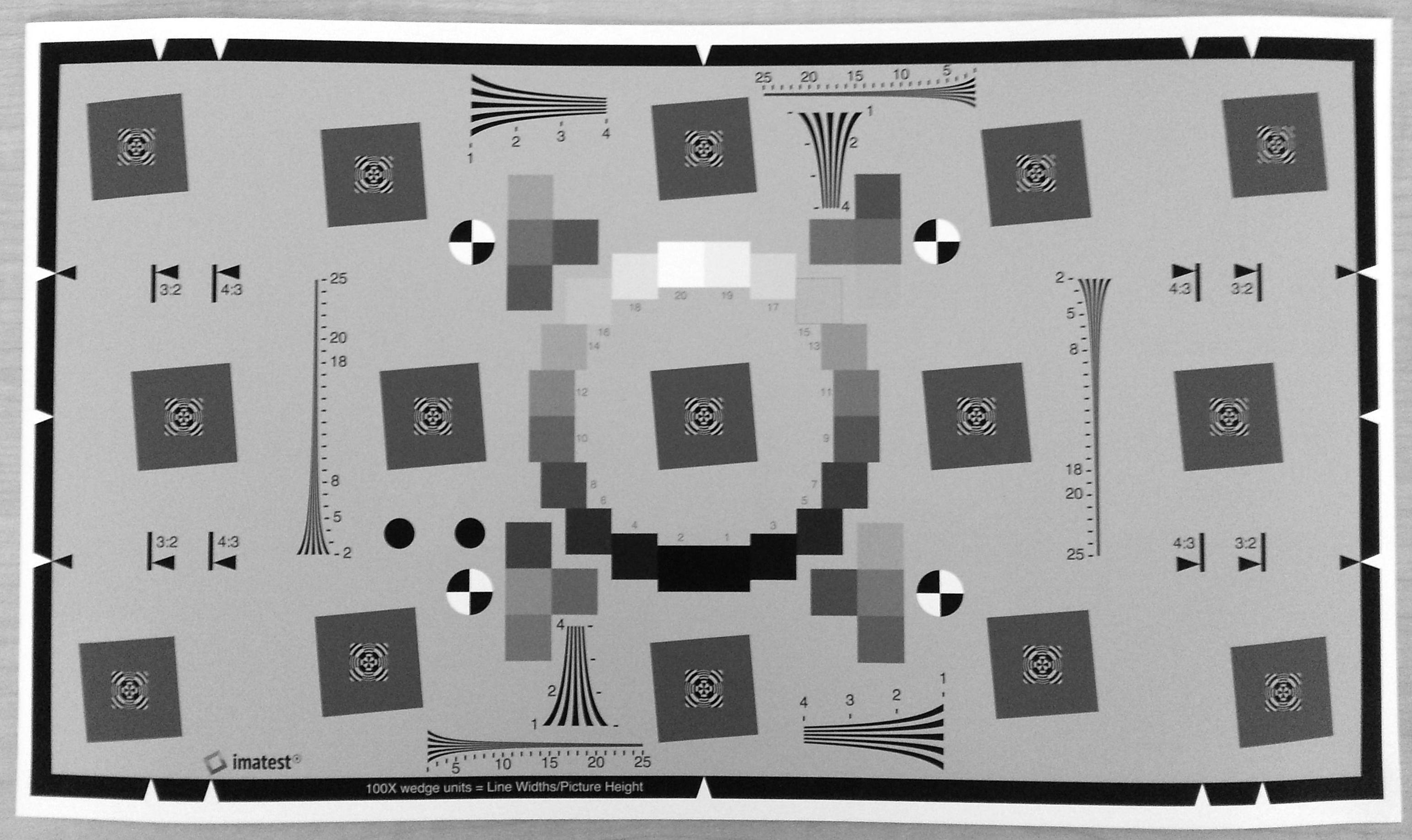
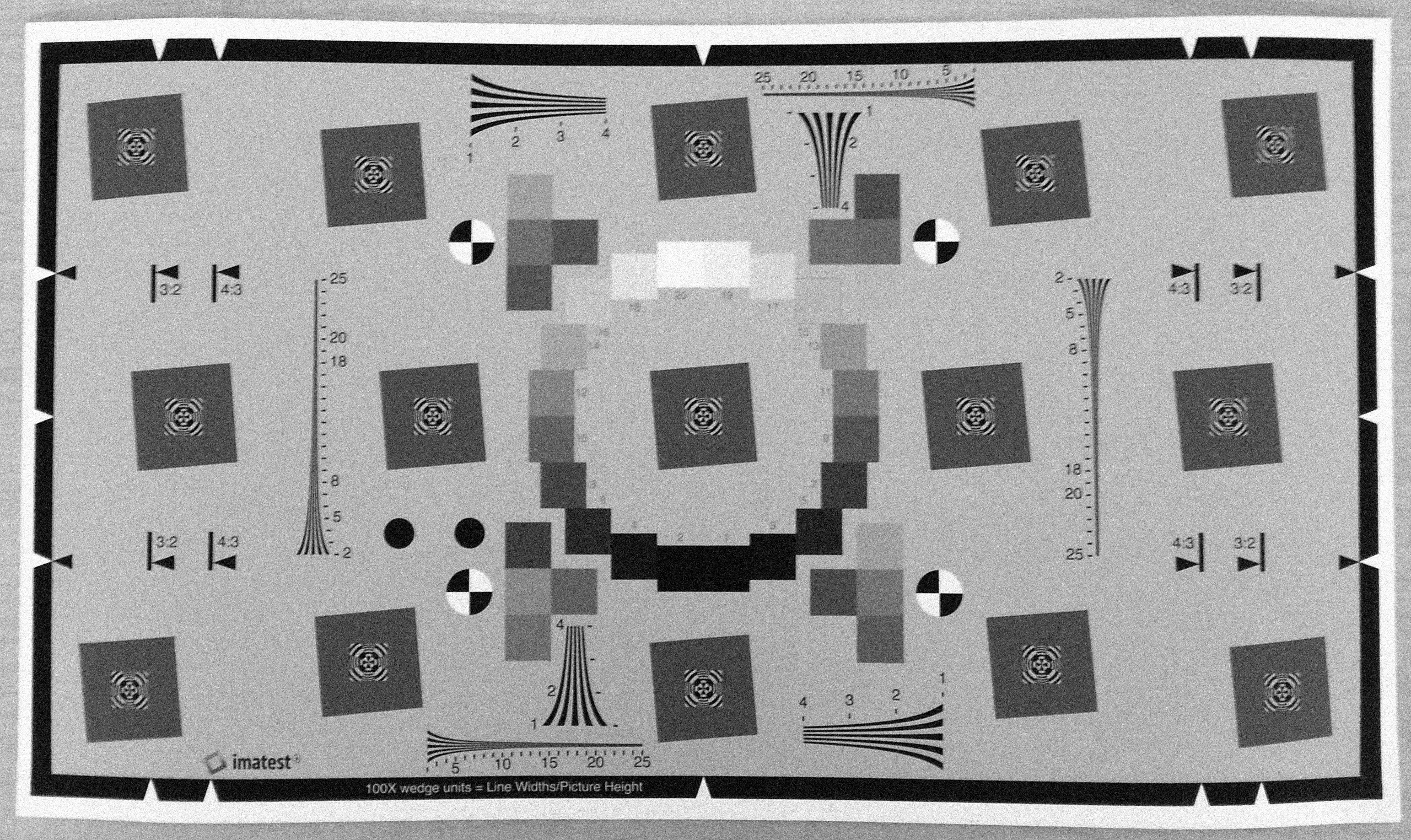
Figure 1: On the left we show Matlab’s test image eSFRTestImage.jpg representing $\mathbf{x}_{\rm true}$, on the right we depict noisy observations represented by $\mathbf{b}$ with $10$% Gaussian white noise which yields an SNR of $20$.

In a first experiment we investigate the convergence of vpal, compared to admm. We consider an image denoising problem with $\mathbf{A}=\mathbf{I}_{n}$, while $\mathbf{b}$ is a Matlab test image eSFRTestImage.jpg of size $1,\!836\times 3,\!084$, so that $\mathbf{x}_{\rm true}$ is of size $n=16,\!986,\!672$, see Fig. 1, left panel. We contaminate $\mathbf{x}_{\rm true}$ with $10$% Gaussian white noise, which yields an SNR of $20$, see Fig. 1 right panel. Here, we utilize a total variation regularization where $\mathbf{D}$ is the 2D finite difference matrix. We fix the regularization parameter as $\mu=10$, select a stopping tolerance $\tau=10^{-4}$, and observe the relative error $e(\mathbf{x}_{k})$ and relative residual $r(\mathbf{x}_{k})$ within iterations $k$ for both methods. The final approximations are denoted by $\mathbf{x}_{\tt vpal}$ and $\mathbf{x}_{\tt admm}$ with reconstruction errors $e(\mathbf{x}_{\tt vpal})=2.890\cdot 10^{-2}$ and $e(\mathbf{x}_{\tt admm})=2.887\cdot 10^{-2}$, respectively. Results are displayed in Fig. 2, where it is shown that admm reaches the solution in fewer iterations than vpal, $28$ to $38$ iterations, respectively. The number of outer iterations used in Algorithms 1 and 2 is, however, an ambiguous computational currency. Following the discussion above, the main computational cost of admm is the number of LSQR iterations utilized for each outer iteration $k$.

Notice vpal has the equivalent computational complexity of only one LSQR solve per iteration $k$. Factoring in these computational costs, we notice that admm overall requires $141$ LSQR iterations while vpal requires $38$ computations, indicating almost a factor of four improvement in the total number of LSQR iterations. Consequently we expect vpal to converge more rapidly.

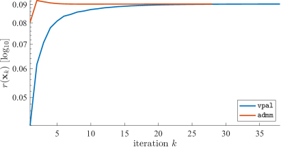
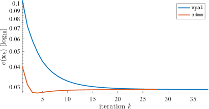
Figure 2: The left panel displays the relative residual , while the right panel depicts the relative error for vpal in blue and admm in red. Both methods converge to an approximation of $\mathbf{x}_{\rm true}$ where the relative difference between admm and vpal is negligible.

Along this line, we extend our investigations and examine wallclock times, see Fig. 3. Using the same computational setup as before, we consider varying sizes of the image in Fig. 1, left panel. Note that in this setup we also slightly vary the regularization parameter $\mu\in[1,20]$ to obtain more realistic timings for “near optimal” regularization parameters. Additionally, in our comparison we include timings for a generalized Tikhonov approach of the form Eq. 3. Here this is referred to as tik, and can be see as a computational lower bound for vpal and admm (left). The Tikhonov problem is solved using LSQR. Notice our comparison to a generalized Tikhonov approach comes with an asterisk, because (1) the range of good regularization parameters is largely different (to obtain close to optimal regularization parameters we choose $\widetilde{\mu}\in[0.1,0.4]$) and (2) the Tikhonov approach leads to inferior reconstructions. Nevertheless, we confirm that despite its computational superiority, vpal does not lack numerical accuracy in comparison to admm. We depict the relative errors $e(\mathbf{x}_{{\tt vpal}})$, $e(\mathbf{x}_{\tt admm})$, and $e(\mathbf{x}_{\tt tik})$ in Fig. 3 right panel.

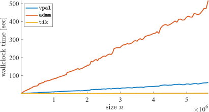
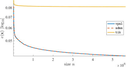
Figure 3: The left plot shows the wallclock timing of vpal (blue), admm (red), and tik (yellow) with increasing image size $n$. Depicted on the right are the corresponding relative reconstruction errors. Despite their differences in computational complexity, both vpal and admm produce nearly identical reconstructions and are virtually indistinguishable, while tik generates inferior reconstructions.

In Fig. 4 we show the average gain in computational speed-up of vpal as compared to admm. Depicted is the ratio of the wallclock timing (admm$/$vpal) in black, confirming the computational advantage of vpal with an approximate average speed-up of about 8. Additionally, we recorded the ratio of how many $\mathcal{O}((m+\ell)n)$ operations (the main computational costs of LSQR equivalent steps) on average each of the methods requires (admm$/$vpal) highlighted in purple. Note, due to the similar curves in Fig. 4, we empirically confirm that the computational costs are dominated by the LSQR solves. Hence, this denoising experiment illustrates that vpal compared to admm reconstructs images accurately at reduced computational cost. We further continue our numerical investigations on tomography applications.

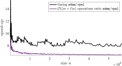
Figure 4: Depicted is the computational gain of vpal compared to admm. In black we show the timing ratio vpal/admm and in violet the ratio of $\mathcal{O}((m+\ell)n)$ operations (main computational cost) of admm compared to vpal.

5.2 3D Medical Tomography

To demonstrate the scalability of our vpal method, we consider a 3D medical tomography application. As a ground truth we consider the 3D Shepp-Logan phantom, illustrated in Fig. 5 (left panel) by slice planes. For the discretization of the Shepp-Logan phantom we use $255\times 255\times 255$ uniform cells, corresponding to $\mathbf{x}_{\rm true}\in\mathbb{R}^{16,581,375}$. Data is generated by a parallel beam tomography setup using the tomobox toolbox [44]. We constructed projection images from $100$ random directions each of size $255\times 255$. The projection images are contaminated with $5\%$ white noise, an SNR of approximately $26$, see four sample projection images in Fig. 6. Consequently, the ray-tracing matrix $\mathbf{A}$ is of size $6,\!502,\!500\times 16,\!581,\!375$. Note that $\mathbf{A}$ is underdetermined and therefore is outside the scope of Theorem 4.7 without convergence guarantees. As the regularization operator we use total variation. Here $\mathbf{D}$ is of size $49,\!549,\!050\times 16,\!581,\!375$ and uses zero boundary conditions. The regularization parameter is set to $\mu=5$.

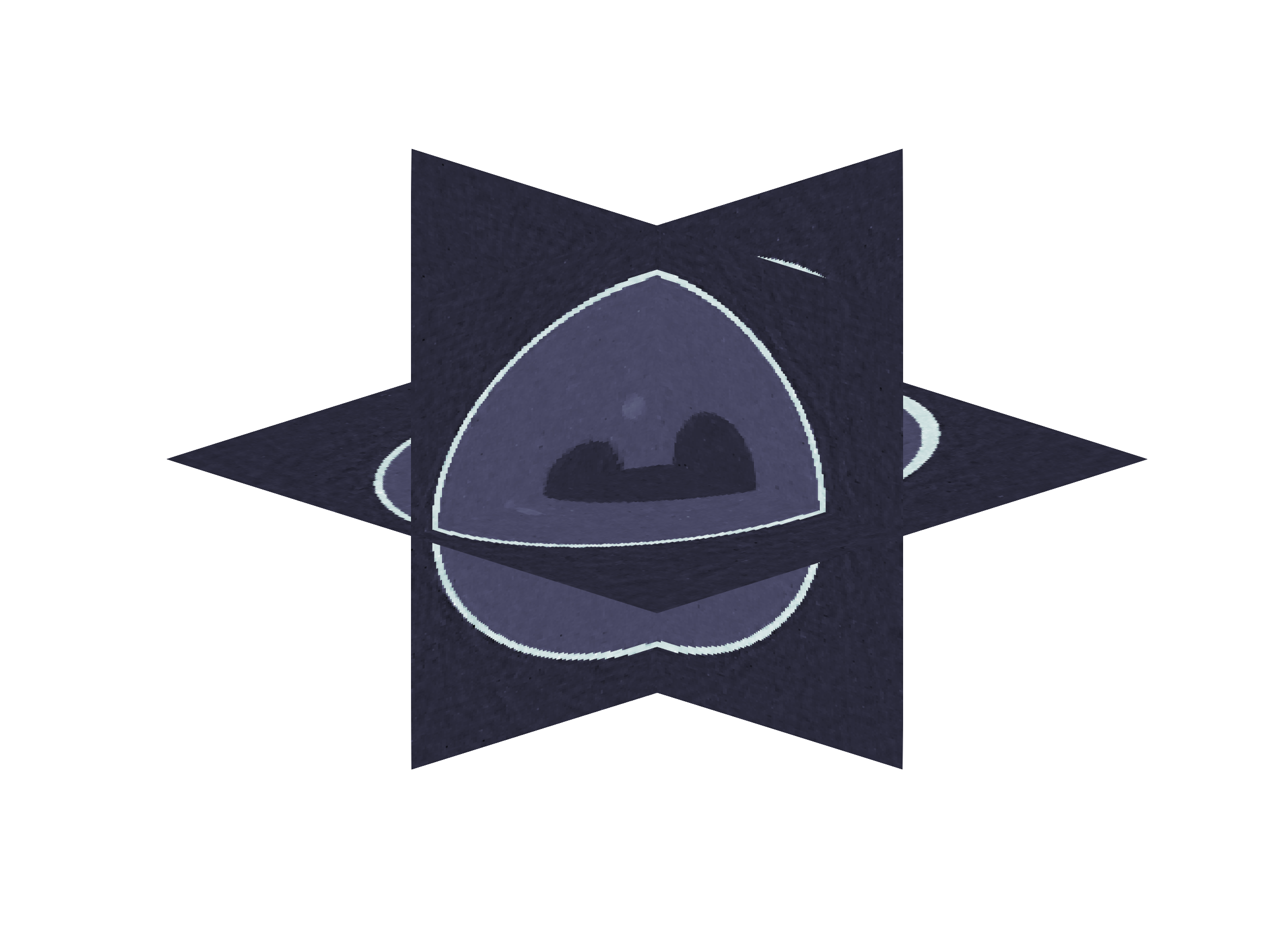
Figure 5: The left panel illustrates the 3D Shepp-Logan phantom using slice planes, while the right panel shows the reconstructed Shepp-Logan phantom using vpal.

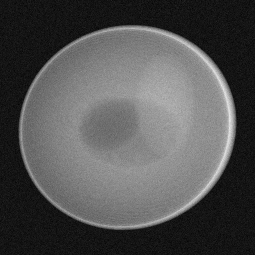
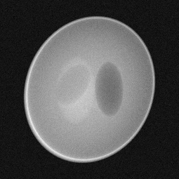
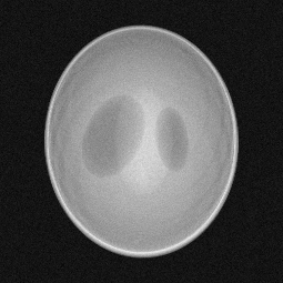
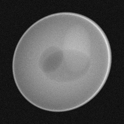
Figure 6: Shown four projection images with $5\%$ white noise and an SNR of approximately $26$.

Our computations were performed on a 2013 MacPro with a 2.7 GHz 12-core Intel Xeon E5 processor with 64 GB Memory 1866 MHz DDR3 running with macOS Big Sur and Matlab 2021a. We use vpal with its default tolerance set to $\tau=10^{-6}$. Our method requires $414$ iterations to converge within the given tolerance with a wallclock time of about $2.4$ hours. The reconstructed 3D Shepp-Logan phantom $\mathbf{x}_{\tt vpal}$ is illustrated in Fig. 5 (right panel) by slice planes. The corresponding relative error is $e(\mathbf{x}_{\tt vpal})=0.1167$. A reconstruction error below $12\%$ is noteworthy, considering that the matrix $\mathbf{A}$ is significantly underdetermined. Again, notice that a standard Tikhonov regularization (using $\mathbf{D}=\mathbf{I}_{n}$) using LSQR is significantly faster (about $3.5$ minutes); however, the relative reconstruction error is inferior. The Tikhonov approach does not generate a relative error below $35\%$ even when utilizing an optimal regularization parameter (data not shown).

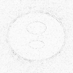
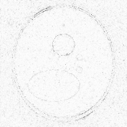
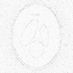
$x$-slice	$y$-slice	$z$-slice

Figure 7: Absolute error of 3D tomography image slices of the reconstruction $\mathbf{x}_{\rm vpal}$ in each principal ($x$, $y$, and $y$) coordinate direction with inverted colormap, where darker gray values correspond to larger absolute errors with largest absolute error of about $0.5346$.

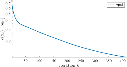
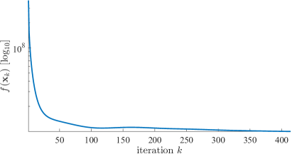
Figure 8: The left graph shows the relative error of the reconstructions $\mathbf{x}_{k}$ at each iteration of vpal of the 3D tomography problem. The right graph shows the corresponding objective function value $f(\mathbf{x}_{k})$ at each iteration. Note that with this under-determined $\mathbf{A}$ the relative error is monotonically decreasing, while the objective function value is not monotonically decreasing.

Reconstruction results are further illustrated in Figs. 7 and 8, where Fig. 7 shows the absolute error image, and Fig. 8 depicts the relative reconstruction errors $\mathbf{x}_{k}$ of vpal and also the corresponding objective function value $f(\mathbf{x}_{k})$ at each iteration. We notice fast but not necessarily monotonically decreasing objective function values $f(\mathbf{x}_{k})$.

5.3 Experiments on parameters

In the following we discuss experiments with our approach for regularization parameter selection using the degrees of freedom argument. As a test bed we investigate a deblurring (blur), 2D medical tomography (tomo), and seismic (seismic) inversion problem. For each problem we utilize the Matlab Toolbox IRtools; see [25] for further details on our choices. Here, in all cases we select Gaussian noise, and for blur we use a severe shake blur for the Hubble space telescope, for tomo we use the 2D Shepp-Logan phantom, while for seismic we select the tectonic phantom. In all usages of the vpal algorithm we select a stopping tolerance of $\tau=10^{-4}$ and limit the number of outer iterations to $1,\!000$. For the bisection algorithm we set $\tau_{1}=0.01$, $\tau_{2}=0.02$, limit the number of bisection steps to $10$, and always use the safety parameter $\eta=1$; no confidence interval is used. Note that each bisection is a full solve of vpal and thus the total maximum number of solves could be as high as $10,\!000$ with these settings. There is a trade-off on the accuracy of the bisection desired and the potential for high computational overhead by carrying out the bisection.

We investigate each of these experiments for various image and data sizes. Our results are presented for four problem sizes with $N$ ranging from $64$ to $512$, corresponding to image sizes $n=N^{2}$ ($4,\!096$, $16,\!384$, $65,\!536$, and $262,\!144$) for problem blur, tomo and seismic. The size of the data vector $\mathbf{b}$ varies with the application, where $m=n$ for blur, $m=16,\!380$, $32,\!580$, $65,\!160$, and $130,\!320$ for tomo and $m=8,\!192$, $32,\!768$, $131,\!072$, and $524,\!288$ for seismic. Notice these experiments correspond to $m=n$ for all the blur cases, $m>n$ for seismic (over-determined) and with tomo $m<n$ (under-determined) for the two larger experiments. In each of these experiments we investigate white noise levels of $10\%$ and $20\%$, corresponding to SNR of $20$ and $13.98$ in each case.

In Figs. 9, 10 and 11 we evaluate the choice of $\mu$ determined using the $\chi^{2}$-DF test to give $\mu_{\textrm{opt}}$ as compared to that obtained as the MAP estimator $\mu_{\textrm{map}}$. To find $\mu_{\textrm{opt}}$ we pick a value for the shrinkage parameter $\gamma$ and estimate $\mu_{\textrm{opt}}$ by the $\chi^{2}$-DF test. (Results show that the $\mu_{\textrm{opt}}$ is virtually independent of $\gamma$.) The relative errors for the solutions obtained in this way are indicated on the plots using the solid red circles with the legend $(\mu_{\textrm{opt}},\gamma)$. We also show the values of the relative error that are obtained by taking $\mu_{\textrm{opt}}$ and $\mu_{\textrm{map}}$, and using the DP to find an optimal $\lambda$, denoted $\lambda_{\textrm{opt}}$ and $\lambda_{\textrm{map}}$ respectively. For the DP we again use the bisection algorithm with all the same settings but now for the function $H(\lambda)=\tfrac{\left\|\mathbf{A}\mathbf{x}(\lambda)-\mathbf{b}\right\|_{2}^{2}}{m\sigma^{2}}-1$. The blue solid circles and green open circles show the errors calculated using the pairs $(\mu_{\textrm{map}},\lambda_{\textrm{map}})$ and $(\mu_{\textrm{opt}},\lambda_{\textrm{opt}})$, respectively, that are generated by $\mu_{\textrm{map}}$ and $\mu_{\textrm{opt}}$, with the DP to find the relevant $\lambda$. Then, given the respective $(\mu,\lambda)$ pairs, we fix $\mu$ but use the $\lambda$ value to provide a range of $\lambda$ logarithmically spaced between $\lambda_{\textrm{map}}/100$ and $100\lambda_{\textrm{map}}$ at $50$ points, with $\lambda_{\textrm{opt}}$ for the $\mu_{\textrm{opt}}$ case. The resulting relative errors obtained for the range of $\lambda$, with fixed $\mu_{\textrm{map}}$ and $\mu_{\textrm{opt}}$, are given in the two curves, blue and red, respectively. In these figures the oscillations in the relative error curves occur if the algorithm did not converge within $1,\!000$ iterations, which is more prevalent for small values of $\lambda$. Given that $\mu$ is fixed on these curves, this corresponds to taking larger values of the shrinkage parameter $\gamma$. Flat portions of the curves indicate the relative lack of sensitivity to the choice of $\lambda$ (respectively $\gamma$) for a fixed $\mu$, equivalently confirming that the optimal $\mu$ is largely independent of $\gamma$ within a suitably determined range, dependent on the data and the problem.

We see immediately that finding $\mu_{\textrm{opt}}$ by the $\chi^{2}$-DF test yields smaller relative errors in the solutions than when the solution is generated using $\mu_{\textrm{map}}$, open green circles and solid red circles are lower than solid blue circles, and except where there are issues with convergence, the red curves lie below blue curves. This is notwithstanding that the $\chi^{2}$-DF test and the MAP estimators do not immediately apply for the tomo and seismic problems, since neither meets the criterion of being differentially Laplacian natural images. Indeed, the Hubble space telescope image is not a perfect example of such an image, but the results demonstrate that the approach still works reasonably well. On the other hand, comparing now red solid and green open circles, contrasts the impact of finding a $\mu_{\textrm{opt}}$ by the $\chi^{2}$-DF test (red solid) and then assessing whether the standard DP (green open) on $\lambda$ might be a better option. It is particularly interesting that the $\chi^{2}$-DF test does uniformly well on tomo and seismic problems, but there are a few cases with blur in which the DP finds a $\lambda$ that yields a smaller relative error. Even in these cases, the results are good using the $\chi^{2}$-DF result. In all situations it is clear that we would not expect to find an optimal $\lambda$ that is at the minimum point of the respective relative error curve, but in general the results are acceptably close to these minimum points. Overall, these results support the approach in which we pick a shrinkage parameter $\gamma$ and find $\mu_{\textrm{opt}}$ using the $\chi^{2}$-DF test by bisection. The results presented for the DP approach to find $\lambda$ were provided to contrast the two directions for estimating the parameters. Indeed, it is clear that finding a $\mu$ to fit $F(\mu)$ given by Eq. 23 to $m\sigma^{2}$ and then fitting the residual term there alone, also to $m\sigma^{2}$, by applying DP, will necessarily increase the value of $F(\mu)$. This set of results demonstrates that there is no need to use the DP principle; rather, optimizing based on Eq. 22 is appropriate for all the test problems.

To further assess the validity of this assertion we also performed a parameter sweep over a grid of values for $(\mu,\lambda)$ for the experiments that use $10\%$ noise, corresponding to an SNR of $20$. For each point on the grid we calculated both the relative error $e(\mathbf{x}(\mu,\lambda))$ and the $\chi^{2}$ value, $|F(\mu,\lambda)/m\sigma^{2}-1|$. The left panels and right panels in Figs. 12, 13 and 14 show the contour plots for the relative errors and $\chi^{2}$ estimates, respectively. The red dots correspond to the points with minimum error and the black dots to the points with minimum $\chi^{2}$ value. If they are close we would assert that the $\chi^{2}$ is optimal for finding a good value for $\mu$. In general, the contours are predominantly vertical, confirming that the solutions are less impacted by the choice of $\lambda$ (and hence shrinkage $\gamma$) than of $\mu$. Further, it is necessary to examine the values for the contours, given in the colorbar, in order to assess whether the $\chi^{2}$ is not giving a good solution. From Figs. 12 and 13 we can conclude that the difference in the relative error from using the $\chi^{2}$ estimate for $\mu$ rather than the optimal in terms of the minimal error is small; all values lie within the blue contours. Even for the seismic case shown in Fig. 14 the contour level for the relative error changes only from about $0.06$ to $0.09$. The captions give the actual calculated relative errors for the red and black dots.

$n=64^{2}$	$n=128^{2}$	$n=256^{2}$	$n=512^{2}$
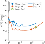
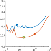
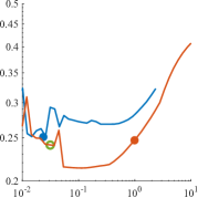
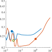
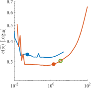
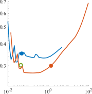
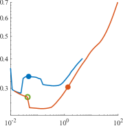
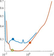
$\lambda$ [log10]	$\lambda$ [log10]	$\lambda$ [log10]	$\lambda$ [log10]

Figure 9: Results for blur example for varying $\lambda$ and fixed regularization parameter $\mu$, $\mu_{\textrm{map}}$ and $\mu_{\textrm{opt}}$ for the blue and red curves, respectively. Also marked for the given fixed $\mu$ choices are the optimal $\lambda$ found using the DP. First row shows relative errors for different image sizes ($n=64^{2},128^{2},256^{2}$, and $512^{2}$) with noise level of $10\%$ corresponding to a signal to noise ratio (SNR) of $20$. Second row shows relative errors with noise level of $20\%$ corresponding to an SNR of $13.98$.

$n=64^{2}$	$n=128^{2}$	$n=256^{2}$	$n=512^{2}$
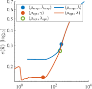
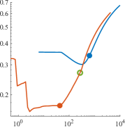
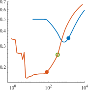
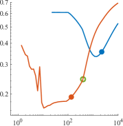
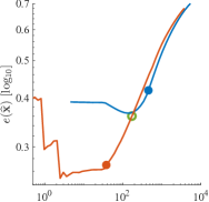
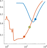
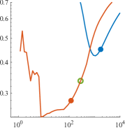
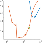
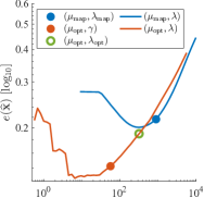
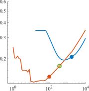
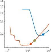
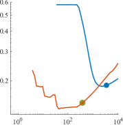
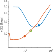
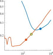
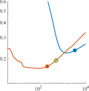
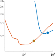
$\lambda$ [log10]	$\lambda$ [log10]	$\lambda$ [log10]	$\lambda$ [log10]

Figure 10: Results for tomo example for varying $\lambda$ and fixed regularization parameter $\mu$, $\mu_{\textrm{map}}$ and $\mu_{\textrm{opt}}$ for the blue and red curves, respectively. Also marked for the given fixed $\mu$ choices are the optimal $\lambda$ found using the DP. First row shows relative errors for different image sizes ($n=64^{2},128^{2},256^{2}$, and $512^{2}$) with noise level of $10\%$ corresponding to a signal to noise ratio (SNR) of $20$. Second row shows relative errors with noise level of $20\%$ corresponding to an SNR of $13.98$.

$n=64^{2}$	$n=128^{2}$	$n=256^{2}$	$n=512^{2}$
$\lambda$ [log10]	$\lambda$ [log10]	$\lambda$ [log10]	$\lambda$ [log10]

Figure 11: Results for seismic example for varying $\lambda$ and fixed regularization parameter $\mu$, $\mu_{\textrm{map}}$ and $\mu_{\textrm{opt}}$ for the blue and red curves, respectively. Also marked for the given fixed $\mu$ choices are the optimal $\lambda$ found using the DP. First row shows relative errors for different image sizes ($n=64^{2},128^{2},256^{2}$, and $512^{2}$) with noise level of $10\%$ corresponding to a signal to noise ratio (SNR) of $20$. Second row shows relative errors with noise level of $20\%$ corresponding to an SNR of $13.98$.

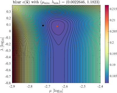
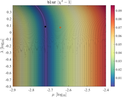
Figure 12: Problem blur: Calculating the relative error and $\chi^{2}$ departure from $m\sigma^{2}$ for a logarithmically uniform grid of points $(\mu,\lambda)$. The minimum relative error is at the red dot and the minimum for the $\chi^{2}$ is at the black dot. The obtained minimum values for the relative errors at these points are $0.1820$ and $0.1840$, and occur for shrinkage parameter $\gamma=0.0016$, and $0.0013$ respectively.

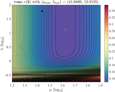
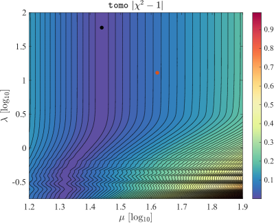
Figure 13: Problem tomo: Calculating the relative error and $\chi^{2}$ departure from $m\sigma^{2}$ for a logarithmically uniform grid of points $(\mu,\lambda)$. The minimum relative error is at the red dot and the minimum for the $\chi^{2}$ is at the black dot. The obtained minimum values for the relative errors at these points are $0.1301$ and $0.1449$, and occur for shrinkage parameter $\gamma=0.2499$, and $0.0076$ respectively.

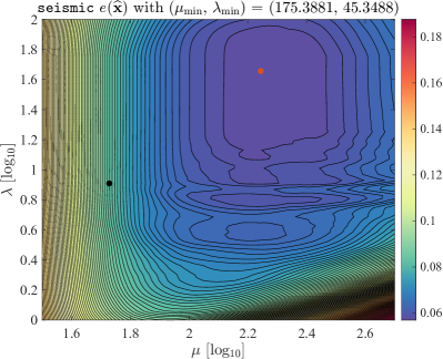
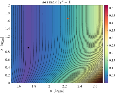
Figure 14: Problem seismic: Calculating the relative error and $\chi^{2}$ departure from $m\sigma^{2}$ for a logarithmically uniform grid of points $(\mu,\lambda)$. The minimum relative error is at the red dot and the minimum for the $\chi^{2}$ is at the black dot. The obtained minimum values for the relative errors at these points are $0.0569$ and $0.0846$, and occur for shrinkage parameter $\gamma=0.0853$, and $0.8125$ respectively.

Finally, to demonstrate the applicability of the bisection algorithm for other differentially Laplacian operators $\mathbf{D}$, we present a small sample of results when $\mathbf{D}$ is the Laplace matrix. We use the same data sets blur, tomo and seismic, with the same noise levels corresponding to SNRs of $20$ and $13.98$, and the same problem sizes, and replace the TV matrix by the Laplace matrix. In Fig. 15, we collect the results in one plot per test, where in each plot we show the relative error curves for a range of $\lambda$ around the optimal $\mu$ for a specific shrinkage parameter $\gamma$ (solid symbols) found using the $\chi^{2}$-DF test. The results again demonstrate the ability of the bisection algorithm with the $\chi^{2}$-DF test to find solutions with near-optimal relative errors.

In summary, we observe empirically that vpal converges particularly fast with only a few iterations, when a near-optimal regularization parameter is selected using the $\chi^{2}$-DF test.

blur	tomo	seismic
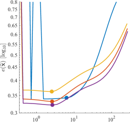
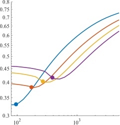
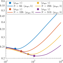
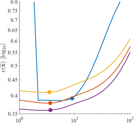
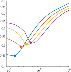
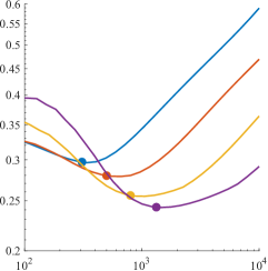
$\lambda$ [log10]	$\lambda$ [log10]	$\lambda$ [log10]

Figure 15: Results for the blur, tomo and seismic problems using the Laplace operator for $\mathbf{D}$. Here blue, red, yellow and purple curves and solid symbols, correspond to results for problems of size $64$, $128$, $256$ and $512$, respectively. The solid symbols indicate the points selected by using the bisection algorithm applied to satisfy the $\chi^{2}$-DF test. The first row shows relative errors with noise level of $10\%$ corresponding to a signal to noise ratio (SNR) of $20$. Second row shows relative errors with noise level of $20\%$ corresponding to an SNR of $13.98$.

6 Discussion & conclusion

In this work we presented a new method for solving generalized total variation problems using an augmented Lagrangian framework that utilizes variable projection methods to solve the inner problem with proven convergence. We further provided an automatic regularization selection method using a degrees of freedom argument. Our investigations included various numerical experiments illustrating the efficiency and effectiveness of our new vpal method for different regularization operators $\mathbf{D}.$

Our work provides a first investigation into the variable projected augmented Lagrangian method, yet many research items remain open. Future research will take multiple directions. First, while Theorem 4.7 provides necessary convergence results, our implementation vpal uses an inexact solve of the inner problem, i.e., a single CG update. We will investigate convergence properties of the inexact approach, utilizing results from inexact ADMM methods [38] for the proof. Second, although we utilize a CG update for the inner iteration, other update strategies may be employed. Since this is a nonlinear problem we may for instance utilize LBFGS updates or nonlinear Krylov subspace methods. Third, estimating a good regularization parameter $\mu$ remains a costly task. In [16] iterative regularization approaches estimating $\mu$ on a subspace were investigated, and demonstrated a computational advantage. We will extend the DF argument to be used to find $\mu$ using a standard bisection algorithm at relatively low cost, when the original model parameters can be assumed to be differentially Laplacian, as is the case for standard image deblurring problems. Fourth, we consider $\ell^{2}-\ell^{1}$ norm regularization here; however, the developed approach extends also to other $\ell^{p}-\ell^{q}$ norm problems [13] and even more general objective functions. We will investigate the convergence and numerical advantages and disadvantages of utilizing a variable projected approach for such $\ell^{p}-\ell^{q}$ problems and for supervised learning loss function fitting within this framework. Fifth, row action methods have been developed to solve least squares and Tikhonov type problems of extremely large-scale where the forward operator $\mathbf{A}$ is too large to keep in computer memory [15, 61]. We will investigate how vpal can be extended to such settings and investigate convergence properties and sampled regularization approaches. Sixth, we will investigate and extend our variable projected optimization method to other suitable optimization problems such as for efficiently solving the Sylvester equations [5].

References

- [1] B. M. Afkham, J. Chung, and M. Chung, Learning regularization parameters of inverse problems via deep neural networks, Inverse Problems, 37 (2021).
- [2] A. Ali and R. J. Tibshirani, The generalized lasso problem and uniqueness, Electronic Journal of Statistics, 13 (2019), pp. 2307–2347.
- [3] J. M. Bardsley, Computational Uncertainty Quantification for Inverse Problems, SIAM, 2018.
- [4] A. Beck and M. Teboulle, A fast iterative shrinkage-thresholding algorithm for linear inverse problems, SIAM Journal on Imaging Sciences, 2 (2009), p. 183–202, https://doi.org/10.1137/080716542.
- [5] P. Benner, R.-C. Li, and N. Truhar, On the adi method for sylvester equations, Journal of Computational and Applied Mathematics, 233 (2009), pp. 1035–1045.
- [6] D. Bertsekas, Nonlinear Programming, Athena Scientific, Belmont, Massachusetts, 1995.
- [7] D. Bertsekas, Constrained Optimization and Lagrange Multiplier Methods, Academic Press, 2014.
- [8] S. Boyd, N. Parikh, E. Chu, B. Peleato, and J. Eckstein, Distributed optimization and statistical learning via the alternating direction method of multipliers, Foundations and Trends® in Machine Learning, 3 (2011), pp. 1–122, https://doi.org/10.1561/2200000016, http://dx.doi.org/10.1561/2200000016.
- [9] S. L. Brunton and J. N. Kutz, Data-driven Science and Engineering: Machine learning, Dynamical systems, and Control, Cambridge University Press, Cambridge, UK, 2019.
- [10] A. Buccini, Fast alternating direction multipliers method by generalized krylov subspaces, Journal of Scientific Computing, 90 (2021), p. 60.
- [11] D. Calvetti and E. Somersalo, An Introduction to Bayesian Scientific Computing: Ten Lectures on Subjective Computing, vol. 2, Springer Science & Business Media, 2007.
- [12] E. J. Candes and T. Tao, Decoding by linear programming, IEEE transactions on information theory, 51 (2005), pp. 4203–4215.
- [13] J. Chung, M. Chung, S. Gazzola, and M. Pasha, Efficient learning methods for large-scale optimal inversion design, arXiv preprint arXiv:2110.02720, (2021).
- [14] J. Chung, M. Chung, and J. T. Slagel, Iterative sampled methods for massive and separable nonlinear inverse problems, in International Conference on Scale Space and Variational Methods in Computer Vision, Springer, 2019, pp. 119–130.
- [15] J. Chung, M. Chung, J. T. Slagel, and L. Tenorio, Sampled limited memory methods for massive linear inverse problems, Inverse Problems, 36 (2020), p. 054001.
- [16] J. Chung and S. Gazzola, Computational methods for large-scale inverse problems: a survey on hybrid projection methods, arXiv preprint 2105.07221, (2021).
- [17] S. Dittmer, T. Kluth, P. Maass, and D. O. Baguer, Regularization by architecture: A deep prior approach for inverse problems, Journal of Mathematical Imaging and Vision, 62 (2020), pp. 456–470.
- [18] C. Dossal, M. Kachour, M. Fadili, G. Peyré, and C. Chesneau, The degrees of freedom of the lasso for general design matrix, Statistica Sinica, 23 (2013), pp. 809–828.
- [19] J. Eckstein and D. P. Bertsekas, On the douglas—rachford splitting method and the proximal point algorithm for maximal monotone operators, Mathematical Programming, 55 (1992), pp. 293–318.
- [20] B. Efron, P. Burman, L. Denby, J. M. Landwehr, C. L. Mallows, X. Shen, H.-C. Huang, J. Ye, J. Ye, and C. Zhang, The estimation of prediction error: Covariance penalties and cross-validation [with comments, rejoinder], Journal of the American Statistical Association, 99 (2004), pp. 619–642, http://www.jstor.org/stable/27590436.
- [21] B. Efron, T. Hastie, I. Johnstone, and R. Tibshirani, Least angle regression, The Annals of Statistics, 32 (2004), pp. 407 – 499, https://doi.org/10.1214/009053604000000067, https://doi.org/10.1214/009053604000000067.
- [22] E. Esser, Applications of lagrangian-based alternating direction methods and connections to split bregman, CAM report, 9 (2009), p. 31.
- [23] M. Fukushima, Application of the alternating direction method of multipliers to separable convex programming problems, Computational Optimization and Applications, 1 (1992), p. 93–111, https://doi.org/10.1007/bf00247655.
- [24] D. Gabay and B. Mercier, A dual algorithm for the solution of nonlinear variational problems via finite element approximation, Computers & Mathematics with Applications, 2 (1976), pp. 17–40.
- [25] S. Gazzola, P. C. Hansen, and J. G. Nagy, IR Tools: a MATLAB package of iterative regularization methods and large-scale test problems, Numerical Algorithms, 81 (2019), pp. 773–811.
- [26] P. Getreuer, Rudin-Osher-Fatemi Total Variation Denoising using Split Bregman, Image Processing On Line, 2 (2012), pp. 74–95. https://doi.org/10.5201/ipol.2012.g-tvd.
- [27] P. E. Gill, W. Murray, and M. H. Wright, Practical Optimization, SIAM, 2019.
- [28] R. Glowinski and A. Marroco, Sur l’approximation, par éléments finis d’ordre un, et la résolution, par pénalisation-dualité d’une classe de problèmes de dirichlet non linéaires, ESAIM: Mathematical Modelling and Numerical Analysis-Modélisation Mathématique et Analyse Numérique, 9 (1975), pp. 41–76.
- [29] T. Goldstein, B. O’Donoghue, S. Setzer, and R. Baraniuk, Fast alternating direction optimization methods, SIAM Journal on Imaging Sciences, 7 (2014), pp. 1588–1623.
- [30] T. Goldstein and S. Osher, The split bregman method for L1-regularized problems, SIAM Journal on Imaging Sciences, 2 (2009), pp. 323–343.
- [31] G. Golub and V. Pereyra, Separable nonlinear least squares: the variable projection method and its applications, Inverse Problems, 19 (2003), p. R1.
- [32] G. H. Golub, M. Heath, and G. Wahba, Generalized cross-validation as a method for choosing a good ridge parameter, Technometrics, 21 (1979), pp. 215–223.
- [33] G. H. Golub and V. Pereyra, The differentiation of pseudo-inverses and nonlinear least squares problems whose variables separate, SIAM Journal on Numerical Analysis, 10 (1973), pp. 413–432.
- [34] E. G. Gol’shtein and N. Tretjiakov, Modified lagrangians in convex programming and their generalizations, in Point-to-Set Maps and Mathematical Programming, Springer, 1979, pp. 86–97.
- [35] M. L. Green, Statistics of images, the tv algorithm of rudin-osher-fatemi for image denoising and an improved denoising algorithm, 2002.
- [36] A. Greenbaum, Iterative Methods for Solving Linear Systems, SIAM, 1997.
- [37] J. Hadamard, Lectures on Cauchy’s Problem in Linear Differential Equations, Yale University Press, New Haven, 1923.
- [38] W. W. Hager and H. Zhang, Inexact alternating direction methods of multipliers for separable convex optimization, Computational Optimization and Applications, 73 (2019), pp. 201–235.
- [39] P. C. Hansen, Rank-deficient and discrete ill-posed problems: numerical aspects of linear inversion, SIAM, 1998.
- [40] P. C. Hansen, Discrete Inverse Problems: Insight and Algorithms, SIAM, 2010.
- [41] P. C. Hansen, J. G. Nagy, and D. P. O’Leary, Deblurring Images: Matrices, Spectra, and Filtering, SIAM, 2006.
- [42] M. R. Hestenes, Multiplier and gradient methods, Journal of Optimization Theory and Applications, 4 (1969), pp. 303–320.
- [43] M. R. Hestenes, E. Stiefel, et al., Methods of conjugate gradients for solving linear systems, vol. 49 (1), NBS Washington, DC, 1952.
- [44] J. Jorgensen, Tomobox. https://www.mathworks.com/matlabcentral/fileexchange/28496-tomobox?s_tid=prof_contriblnk. Accessed: November 2021.
- [45] S.-J. Kim, K. Koh, M. Lustig, S. Boyd, and D. Gorinevsky, An interior-point method for large-scale -regularized least squares, IEEE Journal of Selected Topics in Signal Processing, 1 (2007), pp. 606–617, https://doi.org/10.1109/JSTSP.2007.910971.
- [46] J. L. Mead, Chi-squared test for total variation regularization parameter selection, Inverse Problems & Imaging, 14 (2020), p. 401–421.
- [47] J. L. Mead and R. A. Renaut, A newton root-finding algorithm for estimating the regularization parameter for solving ill-conditioned least squares problems, Inverse Problems, 25 (2008), p. 025002.
- [48] M. A. Meju, Geophysical data analysis: understanding inverse problem theory and practice, Society of Exploration Geophysicists, 1994.
- [49] V. A. Morozov, On the solution of functional equations by the method of regularization, Soviet Mathematics Doklady, 7 (1966), pp. 414–417.
- [50] E. Newman, J. Chung, M. Chung, and L. Ruthotto, slimtrain–a stochastic approximation method for training separable deep neural networks, arXiv preprint arXiv:2109.14002, (2021).
- [51] E. Newman, L. Ruthotto, J. Hart, and B. v. B. Waanders, Train like a (var) pro: Efficient training of neural networks with variable projection, arXiv preprint arXiv:2007.13171, (2020).
- [52] J. Nocedal and S. Wright, Numerical Optimization, Springer Science & Business Media, 2006.
- [53] S. Osher, M. Burger, D. Goldfarb, J. Xu, and W. Yin, An iterative regularization method for total variation-based image restoration, Multiscale Modeling & Simulation, 4 (2005), pp. 460–489.
- [54] D. P. O’Leary and B. W. Rust, Variable projection for nonlinear least squares problems, Computational Optimization and Applications, 54 (2013), pp. 579–593.
- [55] C. C. Paige and M. A. Saunders, Lsqr: An algorithm for sparse linear equations and sparse least squares, ACM Transactions on Mathematical Software (TOMS), 8 (1982), pp. 43–71.
- [56] N. Parikh and S. Boyd, Proximal algorithms, Foundations and Trends in optimization, 1 (2014), pp. 127–239.
- [57] M. J. Powell, A method for nonlinear constraints in minimization problems, Optimization, (1969), pp. 283–298.
- [58] R. A. Renaut, I. Hnětynková, and J. Mead, Regularization parameter estimation for large-scale Tikhonov regularization using a priori information, Computational Statistics and Data Analysis, 54 (2010), pp. 3430 – 3445, https://doi.org/http://dx.doi.org/10.1016/j.csda.2009.05.026, http://www.sciencedirect.com/science/article/pii/S0167947309002278.
- [59] J. C. Santamarina and D. Fratta, Discrete Signals and Inverse Problems: An Introduction for Engineers and Scientists, John Wiley & Sons, 2005.
- [60] J. Sjoberg and M. Viberg, Separable non-linear least-squares minimization-possible improvements for neural net fitting, in Neural Networks for Signal Processing VII. Proceedings of the 1997 IEEE Signal Processing Society Workshop, IEEE, 1997, pp. 345–354.
- [61] J. T. Slagel, J. Chung, M. Chung, D. Kozak, and L. Tenorio, Sampled tikhonov regularization for large linear inverse problems, Inverse Problems, 35 (2019), p. 114008.
- [62] S. M. Stefanov, Separable Programming: Theory and Methods, vol. 53, Springer Science & Business Media, 2001.
- [63] Y. Teng, H. Sun, C. Guo, and Y. Kang, Admm-em method for -norm regularized weighted least squares pet reconstruction, Computational and Mathematical Methods in Medicine, 2016 (2016).
- [64] R. Tibshirani, Regression shrinkage and selection via the lasso, Journal of the Royal Statistical Society: Series B (Methodological), 58 (1996), pp. 267–288.
- [65] R. Tibshirani and L. Wasserman, Sparsity, the lasso, and friends, Lecture notes from “Statistical Machine Learning,” Carnegie Mellon University, Spring, (2017).
- [66] R. J. Tibshirani and J. Taylor, The solution path of the generalized lasso, The Annals of Statistics, 39 (2011), pp. 1335 – 1371, https://doi.org/10.1214/11-AOS878, https://doi.org/10.1214/11-AOS878.
- [67] R. J. Tibshirani and J. Taylor, Degrees of freedom in lasso problems, The Annals of Statistics, 40 (2012), pp. 1198 – 1232, https://doi.org/10.1214/12-AOS1003, https://doi.org/10.1214/12-AOS1003.
- [68] C. Vogel, Computational Methods for Inverse Problems, Society for Industrial and Applied Mathematics, Philadelphia, 2002, https://doi.org/10.1137/1.9780898717570, http://epubs.siam.org/doi/abs/10.1137/1.9780898717570, https://arxiv.org/abs/http://epubs.siam.org/doi/pdf/10.1137/1.9780898717570.
- [69] Y. Wang, W. Yin, and J. Zeng, Global convergence of admm in nonconvex nonsmooth optimization, Journal of Scientific Computing, 78 (2019), pp. 29–63.
- [70] S. J. Wright, Coordinate descent algorithms, Mathematical Programming, 151 (2015), pp. 3–34.
- [71] H. Zou, T. Hastie, and R. Tibshirani, On the “degrees of freedom” of the lasso, The Annals of Statistics, 35 (2007), pp. 2173 – 2192.