Carleman Linearization of Nonlinear Systems and Its Finite-Section Approximations

Abstract

The Carleman linearization is one of the mainstream approaches to lift a finite-dimensional nonlinear dynamical system into an infinite-dimensional linear system with the promise of providing accurate approximations of the original nonlinear system over larger regions around the equilibrium for longer time horizons with respect to the conventional first-order linearization approach. Finite-section approximations of the lifted system has been widely used to study dynamical and control properties of the original nonlinear system. In this context, some of the outstanding problems are to determine under what conditions, as the finite-section order (i.e., truncation length) increases, the trajectory of the resulting approximate linear system from the finite-section scheme converges to that of the original nonlinear system and whether the time interval over which the convergence happens can be quantified explicitly. In this paper, we provide explicit error bounds for the finite-section approximation and prove that the convergence is indeed exponential with respect to the finite-section order. For a class of nonlinear systems, it is shown that one can achieve exponential convergence over the entire time horizon up to infinity. Our results are practically plausible as our proposed error bound estimates can be used to compute proper truncation lengths for a given application, e.g., determining proper sampling period for model predictive control and reachability analysis for safety verifications. We validate our theoretical findings through several illustrative simulations.

34H05, 37M99, 65P99

1 Introduction

For decades, the time-varying and nonlinear nature of most natural, physical, and engineered systems have imposed fundamental challenges on researchers to devise efficient and tractable algorithms to analyze and design such systems. In this work, we are interested in the class of time-varying nonlinear systems whose dynamics are governed by

(1.1) $$\dot{\bf x}(t)={\bf f}(t,{\bf x}(t))$$

for all $t\geq t_{0}$ and ${\bf x}(t_{0})={\bf x}_{0}\neq{\bf 0}$, with the origin ${\bf 0}$ as their equilibrium, where ${\bf x}\in{\mathbb{R}}^{d}$ is the state of the system and ${\bf f}(t,{\bf x})$ is an analytic function about ${\bf x}$ on a neighborhood of the equilibrium ${\bf 0}$. A traditional method to study system (1.1) is the well-known first-order linearization approach that relies on obtaining a linear system from the first-order approximation of the function ${\bf f}(t,{\bf x})$. The first-order linearization approach is valid only when the system is operating near its working point and over a short period of time. To study various properties of nonlinear dynamical systems, researchers have developed several frameworks over the past century [6, 13, 14, 15, 30]. One of mainstream approaches is to lift the finite-dimensional nonlinear system (1.1) into an infinite-dimensional linear system. Carleman linearization and Koopman operator are two of the most prominent methods that are closely connected in spirit [1, 8, 9, 10, 15, 18, 21, 27]. In this paper, we consider Carleman linearization of the nonlinear dynamical system (1.1), quantify several error bounds for its finite-section approximations, and show that the resulting linear systems, for large enough truncation lengths, provide precise approximation to the original nonlinear system on larger neighborhoods around the equilibrium, with respect to the first-order linearization, and for longer periods of time.

The control system community has experienced several success stories through methods that are developed based on Carleman linearization ideas [2, 3, 10, 12, 19, 23, 24, 16, 17, 25]. For instance, the author of [24] identified some connections between Carleman linearization and Lie series, and then utilized it to design optimal control laws for infinite-dimensional systems. Reference [19] exploits Carleman approximation to obtain a relation between the lifted system and the domain of attraction of the original nonlinear system. Recent work [12] employs Carleman linearization to implement model predictive control for nonlinear systems efficiently. In [21], ideas from Carleman linearization are applied for state estimation and design of feedback control laws. By exploiting the inherent structure of the lifted system, the authors of [2, 3] proposed a tractable method to quantilize and solve the Hamilton-Jacobi-Bellman equation through an exact iterative method.

The Carleman linearization of the nonlinear dynamical system (1.1), which is expressed in (2.11), is an infinite-dimensional linear time-varying system, whose state matrix is an upper-triangular block matrix. One should be meticulous in handling the resulting infinite-dimensional linear system since the corresponding state matrix does not represent a bounded operator on the Hilbert space of all square-summable sequences. Moreover, the initial of the linear system has exponential decay when $\|{\bf x}_{0}\|_{\infty}<1$ and exponential growth when $\|{\bf x}_{0}\|_{\infty}>1$, where $\|{\bf x}_{0}\|_{\infty}$ is the maximal norm of the initial ${\bf x}_{0}$. These factors have prevented us from directly applying the existing theory to analyze the resulting linear system from Carleman linearization and then better understand the original nonlinear dynamical system.

A common remedy to deal with the Carleman linearization is finite-section approximations, which is given by (2.13), where one truncates the infinite-dimensional linear system [9, 18, 23]. A fundamental question is whether the first block of the solution of the finite-section approximation converges to the solution of the original nonlinear dynamical system and what the convergence rate is. In this work, we provide a partial answer to the above questions when the coefficients in Maclaurin expansion of the analytic function $f(t,{\bf x})$ enjoys certain uniform decay property, see Assumption 2.1. In our main contribution, it is shown that if the initial condition is in a vicinity of the equilibrium, then the first block of the solution of the finite-section approximation will exponentially converge to the solution of the original nonlinear system as the order of the truncation in the finite-section approximation increases, see Theorems 3.1, 3.4 and 3.5. We highlight that the authors of [9, 18] have established similar convergence result when the function $f(t,{\bf x})$ in (1.1) is a polynomial.

The paper is organized as follows. In Section 2, we consider Carleman linearization of the nonlinear dynamical system (1.1) and its finite section approximation, see (2.11) and (2.13). In Section 3, we establish the exponential convergence of the finite section scheme over some time interval, see Theorem 3.1, Corollary 3.3, and Theorems 3.4 and 3.5. In Section 4, Carleman linearization of several benchmark systems are discussed to validate and illustrate the theoretical findings in Theorems 3.1 and 3.4. The technical proofs of all conclusions are provided in Section 5.

Some preliminary versions of this work were announced in [1, 4]. The authors assert that the content of this manuscript significantly differs from its conference versions as this work contains several new and improved results as well as several new case studies with respect to its conference versions.

2 Carleman Linearization and Its Finite-Section Approximations

We review some notions related to the Carleman linearization and its finite section scheme [4, 5, 9, 10, 18, 21, 23, 24]. For a given vector ${\bf x}=[x_{1},\ldots,x_{d}]^{T}\in{\mathbb{R}}^{d}$, let us denote monomial ${\bf x}_{\boldsymbol{\alpha}}=x_{1}^{\alpha_{1}}\cdots x_{d}^{\alpha_{d}}$ for some ${\boldsymbol{\alpha}}=[\alpha_{1},\ldots,\alpha_{d}]^{T}\in{\mathbb{Z}}_{+}^{d}$, where ${\mathbb{Z}}_{+}^{d}$ is the set of all $d$-dimensional non-negative integer vectors. Suppose that the Maclaurin series of the vector-valued analytic function ${\bf f}(t,{\bf x})$ in (1.1) can be expressed as

(2.1) $${\bf f}(t,{\bf x})=\sum_{{\boldsymbol{\alpha}}\in{\mathbb{Z}}_{+}^{d}\backslash\{{\bf 0}\}}{\bf f}_{\boldsymbol{\alpha}}(t){\bf x}_{\boldsymbol{\alpha}}$$

for all $t\geq t_{0}$. For a given ${\boldsymbol{\alpha}}=[\alpha_{1},\ldots,\alpha_{d}]^{T}\in{\mathbb{Z}}_{+}^{d}$, let us define $|\boldsymbol{\alpha}|=\alpha_{1}+\cdots+\alpha_{d}$ and set ${\mathbb{Z}}_{k}^{d}=\{{\boldsymbol{\alpha}}\in{\mathbb{Z}}_{+}^{d}~{}|~{}|\boldsymbol{\alpha}|=k\}$. In this work, we assume that the coefficients of the Maclaurin series (2.1) have the following uniform exponential decay property; we refer to (3.24) for another conventional uniform exponential decay assumption.

Assumption 2.1.

There exist positive constants $D_{0}$ and $R>0$ such that the coefficients ${\bf f}_{\boldsymbol{\alpha}}(t)=[f_{1,\boldsymbol{\alpha}}(t),\ldots,f_{d,\boldsymbol{\alpha}}(t)]^{T}$ in the Maclaurin expansion (2.1) satisfy

(2.2) $$\sup_{t\geq t_{0}}\sum_{j=1}^{d}\sum_{\boldsymbol{\alpha}\in{\mathbb{Z}}_{k}^{d}}|f_{j,\boldsymbol{\alpha}}(t)|\leq D_{0}R^{-k}$$

for $k\geq 1$.

When ${\bf f}(t,{\bf x})$ in (1.1) is a polynomial of degree $L\geq 1$, i.e.,

(2.3) $${\bf f}(t,{\bf x})={\bf p}_{L}(t,{\bf x})=\sum_{1\leq|\boldsymbol{\alpha}|\leq L}\hskip 1.42271pt[p_{1,\boldsymbol{\alpha}}(t),\ldots,p_{d,\boldsymbol{\alpha}}(t)]^{T}\hskip 0.56917pt{\bf x}^{\boldsymbol{\alpha}},$$

Assumption 2.1 will be satisfied as one can verify that for every convergence radius $R>0$, the uniform exponential decay property (2.2) holds with $D_{0}$ replaced by

(2.4) $$D_{0}({\bf p}_{L},R)=\sup_{1\leq k\leq L}R^{k}\sup_{t\geq t_{0}}\sum_{j=1}^{d}\sum_{\boldsymbol{\alpha}\in{\mathbb{Z}}_{k}^{d}}|p_{j,\boldsymbol{\alpha}}(t)|.$$

Let us denote the standard Euclidean basis for $\mathbb{R}\,^{d}$ by ${\bf e}_{1},\ldots,{\bf e}_{d}$ and set

(2.5) $$f_{j,\boldsymbol{\alpha}}(t)=0$$

for all $\boldsymbol{\alpha}\not\in{{\mathbb{Z}}}_{+}^{d}\backslash\{{\bf 0}\}$ and $j=1,\ldots,d$. The Carleman linearization of the nonlinear dynamical system (1.1) starts from its reformulation

(2.6) $$\dot{x}_{j}(t)=\sum_{{\boldsymbol{\alpha}}\in{\mathbb{Z}}_{+}^{d}\backslash\{{\bf 0}\}}f_{j,{\boldsymbol{\alpha}}}(t)\hskip 1.42271pt{\bf x}_{\boldsymbol{\alpha}}(t)$$

for $j=1,\ldots,d$. For every $\boldsymbol{\alpha}=[\alpha_{1},\ldots,\alpha_{d}]\in{\mathbb{Z}}_{+}^{d}\backslash\{{\bf 0}\}$, the derivative of monomial ${\bf x}_{\boldsymbol{\alpha}}$ can be calculated as

$$\dot{{\bf x}}_{\alpha}(t) = \sum_{j=1}^{d}~{}\alpha_{j}{\bf x}_{\boldsymbol{\alpha}-{\bf e}_{j}}\sum_{\boldsymbol{\gamma}\in{\mathbb{Z}}_{+}^{d}\backslash\{{\bf 0}\}}f_{j,\boldsymbol{\gamma}}(t)\hskip 1.42271pt{\bf x}_{\boldsymbol{\gamma}}(t)$$

$$= \sum_{\boldsymbol{\beta}\in{\mathbb{Z}}_{+}^{d}\backslash\{{\bf 0}\}}\left(\sum_{j=1}^{d}\alpha_{j}f_{j,\boldsymbol{\beta}-\boldsymbol{\alpha}+{\bf e}_{j}}(t)\right){\bf x}_{\boldsymbol{\beta}}(t),$$

with initial condition ${\bf x}_{\boldsymbol{\alpha}}(t_{0})=({\bf x}_{0})_{\boldsymbol{\alpha}}$. For every $k\geq 1$, we define a new state variable as ${\bf z}_{k}=[{\bf x}_{\boldsymbol{\alpha}}]_{{\boldsymbol{\alpha}}\in{\mathbb{Z}}_{k}^{d}}$, which contains all the monomials of order $k$. Regrouping monomials in (2) all together yields the following infinite-dimensional linear system

(2.8) $$\dot{\bf z}_{k}(t)=\sum_{l=k}^{\infty}{\bf A}_{k,l}(t)\hskip 1.42271pt{\bf z}_{l}(t)\ \ {\rm and}\ \ {\bf z}_{k}(t_{0})=\big{[}{\bf x}^{0}_{\boldsymbol{\alpha}}\big{]}_{{\boldsymbol{\alpha}}\in{\mathbb{Z}}_{k}^{d}}$$

for all $t\geq t_{0}$ and $k\geq 1$, where

(2.9) $${\bf A}_{k,l}(t)=\left[\sum_{j=1}^{d}\alpha_{j}f_{j,\boldsymbol{\beta}-\boldsymbol{\alpha}+{\bf e}_{j}}(t)\right]_{{\boldsymbol{\alpha}}\in{\mathbb{Z}}_{k}^{d},~{}{\boldsymbol{\beta}}\in{\mathbb{Z}}_{l}^{d}}$$

are matrices of size ${{k+d-1}\choose d-1}\times{{l+d-1}\choose d-1}$. By defining the infinite-dimensional state vector

(2.10) $${\bf z}=[{\bf z}_{1},{\bf z}_{2},\ldots,{\bf z}_{N},\ldots]^{T},$$

the set of linear systems (2.8) can be rewritten in the following infinite-dimensional matrix form

(2.11) $$\dot{\bf z}(t)={\bf A}(t){\bf z}(t)$$

for all $t\geq t_{0}$ with the initial condition ${\bf z}(t_{0})=[{\bf z}_{k}(t_{0})]_{k\geq 1}$, where

(2.12) $${\bf A}(t)=\left[\begin{array}[]{ccccc}{\bf A}_{1,1}(t)&{\bf A}_{1,2}(t)&\cdots&{\bf A}_{1,N}(t)&\cdots\\ &{\bf A}_{2,2}(t)&\cdots&{\bf A}_{2,N}(t)&\cdots\\ &&\ddots&\vdots&\ddots\\ &&&{\bf A}_{N,N}(t)&\cdots\\ &&&&\ddots\end{array}\right].$$

The resulting linear system (2.11) is referred to as Carleman linearization of the nonlinear dynamical system (1.1). While the state-space of the original nonlinear system (1.1) is the finite-dimensional Euclidean space $\mathbb{R}\,^{d}$, its Carleman linearization (2.11) is an infinite-dimensional linear time-varying system whose state matrix ${\bf A}(t)$ is an upper-triangular block matrix. According to the bound estimates for the block matrices ${\bf A}_{k,l}(t)$ for all $1\leq k\leq l$ in Lemma 5.1, the state matrix ${\bf A}(t)$ in (2.11) is not a bounded operator on $\ell^{2}({\mathbb{Z}}_{+}^{d}\backslash\{{\bf 0}\})$, the Hilbert space of all square-summable sequences on ${\mathbb{Z}}_{+}^{d}\backslash\{{\bf 0}\}$. Moreover, it is observed that its initial ${\bf z}(t_{0})$ has exponential decay when $\|{\bf x}_{0}\|_{\infty}<1$ and exponential growth when $\|{\bf x}_{0}\|_{\infty}>1$, in which the maximal norm of a vector ${\bf x}=[x_{1},\ldots,x_{d}]^{T}\in{\mathbb{R}}^{d}$ is represented by $\|{\bf x}\|_{\infty}=\max_{1\leq j\leq d}|x_{j}|$. The above two observations have been the main preventive factors to apply existing theory on Hilbert space directly to analyze the Carleman linearization of a nonlinear system.

A conventional approach to solve the infinite-dimensional linear system (2.11) is to consider its finite-section approximation of order $N$, which is given by

(2.13) $$\left[\begin{array}[]{c}\dot{\bf y}_{1,N}(t)\\ \dot{\bf y}_{2,N}(t)\\ \vdots\\ \dot{\bf y}_{N,N}(t)\end{array}\right]=\left[\begin{array}[]{ccccc}{\bf A}_{1,1}(t)&{\bf A}_{1,2}(t)&\cdots&{\bf A}_{1,N}(t)\\ &{\bf A}_{2,2}(t)&\cdots&{\bf A}_{2,N}(t)\\ &&\ddots&\vdots\\ &&&{\bf A}_{N,N}(t)\end{array}\right]\left[\begin{array}[]{c}{\bf y}_{1,N}(t)\\ {\bf y}_{2,N}(t)\\ \vdots\\ {\bf y}_{N,N}(t)\end{array}\right]$$

with initial ${\bf y}_{k,N}(t_{0})={\bf z}_{k}(t_{0})$ for $k=1,\ldots,N$ [9, 18, 20, 21]. The above finite-section scheme is of dimension ${{N+d}\choose d}-1$ and can be solved by first solving

$$\dot{\bf y}_{N,N}(t)={\bf A}_{N,N}(t){\bf y}_{N,N}(t)\ \ {\rm with}\ \ y_{N,N}(t_{0})={\bf z}_{N}(t_{0})$$

and then solving

$$\dot{\bf y}_{k,N}(t)={\bf A}_{k,k}(t){\bf y}_{k,N}(t)+\sum_{l=k+1}^{N}{\bf A}_{k,l}(t){\bf y}_{l,N}(t)\ \ {\rm with}\ \ y_{k,N}(t_{0})={\bf z}_{k}(t_{0})$$

for $k=N-1,\ldots,1$, recursively, where the size of each subsystem is ${{k+d-1}\choose{d-1}}$. For $N=1$, the finite-section approximation (2.13) becomes the well-known first-order linearization of the nonlinear system (1.1) that has been widely used in practice. The first block of the state vector in the linear system (2.11) corresponds to the solution of the original nonlinear system. When considering the finite-section approximation (2.13), it is desirous to scrutinize whether the first block of its solution converges to the solution of the original nonlinear system (1.1) and what the convergence rate is. In the next section, we provide partial answers to the above query when the function $f(t,{\bf x})$ in (1.1) satisfies Assumption 2.1; c.f. [9, 18] where $f(t,{\bf x})$ is a polynomial.

3 Convergence of Finite-Sectioning of the Carleman Linearization

In this part, we study convergence properties of the finite-section approximation (2.13) of the Carleman linearization (2.11). Theorem 3.1 shows that if the initial condition ${\bf x}_{0}$ satisfies

(3.1) $$0<\|{\bf x}_{0}\|_{\infty}<R/e,$$

then the first block ${\bf y}_{1,N}(t)$ for $N\geq 1$, of the solution of the finite-section approximation (2.13) converges exponentially to the true solution ${\bf x}(t)$ of the nonlinear dynamical system (1.1) over time interval $[t_{0},t_{0}+T^{*})$, where $D_{0}$ and $R$ are the constants in Assumption 2.1 and

(3.2) $$T^{*}=\frac{(e-1)R}{(2e-1)D_{0}}\ln\left(\frac{R}{e\|{\bf x}_{0}\|_{\infty}}\right).$$

In [9, Theorem 4.2], the authors consider a special case of this problem when $f(t,{\bf x})$ is a time-independent polynomial. This implies that finite-section approximation of the Carleman linearization provides a reasonable approximation of the original nonlinear system over a quantifiable time interval that depends linearly on the logarithmic scale of the distance of the initial from the equilibrium.

Furthermore, we are interested in those nonlinear systems (1.1) with the following additional property on their Jacobian $\nabla{\bf f}(t,{\bf 0})=[{\bf f}_{{\bf e}_{1}}(t),\ldots,{\bf f}_{{\bf e}_{d}}(t)]^{T}$ at the equilibrium ${\bf 0}$.

Assumption 3.1.

The Jacobian $\nabla{\bf f}(t,{\bf 0})$ is a time-independent diagonal matrix with negative diagonal entries $\lambda_{\boldsymbol{\alpha}}$ for every $|\boldsymbol{\alpha}|=1$ that satisfy

(3.3) $$\lambda_{\boldsymbol{\alpha}}\leq-\mu_{0}~{}~{}{\rm for\ all}~{}~{}|\boldsymbol{\alpha}|=1$$

for some $\mu_{0}>0$.

In Theorem 3.4, we show that if the initial condition ${\bf x}_{0}$ satisfies

(3.4) $$0<\|{\bf x}_{0}\|_{2}<\frac{R^{2}\mu_{0}}{D_{0}+R\mu_{0}},$$

where $\|{\bf x}_{0}\|_{2}$ is the Euclidean norm of ${\bf x}_{0}$, then the first block ${\bf y}_{1,N}$ of the solution of the finite-section approximation (2.13) of the Carleman linearization (2.11) will converge exponentially to the true solution of the nonlinear dynamical system (1.1) over the entire time interval $[t_{0},\infty)$, where $D_{0},R,\mu_{0}$ are the constants in Assumptions 2.1 and 3.1; cf. [18, Corollary 1 in the Supplementary Information] for the case that $f(t,{\bf x})$ is a polynomial. It is observed from Corollary 5.13 that the nonlinear dynamical system (1.1) with the analytic function ${\bf f}(t,{\bf x})$ satisfying Assumptions 2.1 and 3.1 is stable when the initial ${\bf x}(t_{0})={\bf x}_{0}$ satisfies (3.4). Despite the traditional first-order linearization approach that results in approximations that are useful only over short time intervals, we demonstrate that the Carleman linearization can be employed over the entire time horizon when the origin is an asymptotically stable equilibrium of the nonlinear dynamical system.

The next theorem is the first main contribution of this work, where its proof is given in Section 5.1 and a couple of supporting numerical examples are demonstrated in Section 4.

Theorem 3.1.

Suppose that ${\bf x}(t)$ is the solution of the nonlinear dynamical system (1.1), the analytic function ${\bf f}(t,{\bf x})$ in (1.1) satisfies Assumption 2.1, and ${\bf y}_{1,N}(t)$ for every $N\geq 1$ is the first block of the solution of the finite-section approximation (2.13). If the initial ${\bf x}(t_{0})={\bf x}_{0}$ satisfies (3.1), then

(3.5) $$\|{\bf y}_{1,N}(t)-{\bf x}(t)\|_{\infty}\leq\frac{RM_{0}}{\sqrt{2\pi}(R-M_{0})}N^{-3/2}e^{D_{0}(t-t_{0})N/R}\left(\frac{\|{\bf x}_{0}\|_{\infty}e}{R}\right)^{(e-1)N/(2e-1)}$$

holds for all $t_{0}\leq t\leq t_{0}+T^{*}$ and $N\geq 1$, where $T^{*}$ is defined by (3.2) and

(3.6) $$M_{0}=\|{\bf x}_{0}\|_{\infty}^{(e-1)/(2e-1)}(R/e)^{e/(2e-1)}<R/e.$$

An important step in the proof of Theorem 3.1 is to establish the local bound estimate

(3.7) $$\|{\bf x}(t)\|_{\infty}\leq M_{0}\ \ {\rm for\ all}\ \ t_{0}\leq t\leq t_{0}+T^{*}.$$

We refer to Lemma 5.3 for more details. Whenever a local bound for the solution ${\bf x}(t)$ for all $t\geq t_{0}$ is provided a priori, i.e., there exist an upper bound $M<R/e$ and a time range $T_{1}>0$ such that

(3.8) $$\|{\bf x}(t)\|_{\infty}\leq M\ \ {\rm for\ all}\ \ t_{0}\leq t\leq t_{0}+T_{1},$$

one can apply a similar argument to establish the following result.

Corollary 3.2.

Suppose that the solution ${\bf x}(t)$ of the nonlinear dynamical system (1.1) satisfies (3.8), and the analytic function ${\bf f}(t,{\bf x})$ in (1.1) satisfies Assumption 2.1. Then

(3.9) $$\|{\bf y}_{1,N}(t)-{\bf x}(t)\|_{\infty}\leq\frac{RM}{\sqrt{2\pi}(R-M)}N^{-3/2}\left(\frac{M\exp(D_{0}(t-t_{0})/R+1)}{R}\right)^{N}$$

holds for all $t_{0}\leq t\leq t_{0}+\tilde{T}^{*}$ and $N\geq 1$, where $M,D_{0},R$ are constants in (3.8) and Assumption 2.1 and

(3.10) $$\tilde{T}^{*}=\min\left\{T_{1},\frac{R}{D_{0}}\ln\frac{R}{Me}\right\}.$$

As a consequence of Theorem 3.1, one has the following result for systems (1.1) whose right-hand side is a polynomial described by (2.3); cf. [9, Theorem 4.2].

Corollary 3.3.

Let us consider the nonlinear system (1.1) with a nonzero initial ${\bf x}(t_{0})={\bf x}_{0}\neq 0$, where its ${\bf f}(t,{\bf x})$ is a polynomial as in (2.3) of order $L\geq 2$, and set

(3.11) $$T^{*}({\bf p}_{L},{\bf x}_{0})=\sup_{R>e\|{\bf x}_{0}\|_{\infty}}\frac{(e-1)R}{(2e-1)D_{0}({\bf p}_{L},R)}\ln\left(\frac{R}{e\|{\bf x}_{0}\|_{\infty}}\right),$$

where $D_{0}({\bf p}_{L},R)$ is given by (2.4). Then, the first block ${\bf y}_{1,N}(t)$ of the solution of the finite-section approximation (2.13) converges exponentially to the solution ${\bf x}(t)$ of the original nonlinear system (1.1) for all $t_{0}<t<t_{0}+T^{*}({\bf p}_{L},{\bf x}_{0})$.

In order to calculate the maximal achievable time range from (3.11), we define

$$a_{k}=\sup_{t\geq t_{0}}\sum_{j=1}^{d}\sum_{\boldsymbol{\alpha}\in{\mathbb{Z}}_{k}^{d}}|p_{j,\boldsymbol{\alpha}}(t)|$$

for all $k=1,\ldots,L$. For all $R\geq\max_{1\leq k\leq L-1}(a_{k}/a_{L})^{1/(L-k)}$, one may verify that $D_{0}({\bf p}_{L},R)=a_{L}R^{L}$. Hence, whenever $\|{\bf x}_{0}\|_{\infty}\geq e^{-1}\max_{1\leq k\leq L-1}(a_{k}/a_{L})^{1/(L-k)}$, we should select $R\geq\max_{1\leq k\leq L-1}(a_{k}/a_{L})^{1/(L-k)}$, which as a result the maximal achievable time range according to (3.11) can be found as

$$T^{*}({\bf p}_{L},{\bf x}_{0}) = \frac{e-1}{(2e-1)a_{L}}\sup_{R>e\|{\bf x}_{0}\|_{\infty}}R^{1-L}\ln\left(\frac{R}{e\|{\bf x}_{0}\|_{\infty}}\right)$$

$$= \frac{e-1}{(2e-1)(L-1)e^{L}a_{L}}\|{\bf x}_{0}\|_{\infty}^{1-L}.$$

The last equality in (3) follows as it can be verified that $R^{1-L}(\ln R-\ln\|{\bf x}_{0}\|_{\infty}-1)$ takes its maximal values at $R=e^{L/(L-1)}\|{\bf x}_{0}\|_{\infty}$. We remark that whenever the polynomial ${\bf p}_{L}(t,{\bf x})$ in (2.3) for $L\geq 2$ is time-independent, the authors of [9] provide an estimate for the maximal time range $T^{*}$ similar to the one in (3); we refer to [9, Theorem 4.3].

By Theorem 3.1, the first block of the solution of the finite section scheme (2.13) enjoys exponential convergence to the true solution over a quantifable period of time. In [18], the authors consider the nonlinear dynamical system (1.1) with ${\bf f}(t,{\bf x})$ being a polynomial ${\bf p}_{L}(t,{\bf x})$ as in (2.3) with $L=2$. Under the assumptions that the gradient $\nabla{\bf f}(t,{\bf 0})$ is time-independent, diagonalizable, and has eigenvalues that have negative real parts, c.f. Assumption 3.1, they show that the first block of the solution of the finite-section approximation (2.13) converges exponentially to the solution ${\bf x}(t)$ of the nonlinear dynamical system (1.1) on the whole time range $t\geq t_{0}$ when the initial ${\bf x}_{0}$ is not too far away from the origin. In the next theorem, which is our second main contribution of this work, we consider exponential convergence of the first block of the solution of the finite-section approximation (2.13) over the entire time horizon from $t_{0}$ to $\infty$, where ${\bf f}(t,{\bf x})$ in (1.1) satisfies Assumptions 2.1 and 3.1.

Theorem 3.4.

Suppose that ${\bf x}(t)$ is the continuous solution of nonlinear system (1.1) and the analytic function ${\bf f}(t,{\bf x})$ in (1.1) satisfy Assumptions 2.1 and 3.1. If the initial ${\bf x}(t_{0})={\bf x}_{0}$ satisfies (3.4), then

(3.13) $$\|{\bf y}_{1,N}(t)-{\bf x}(t)\|_{\infty}\leq\|{\bf x}_{0}\|_{2}\left(\frac{(D_{0}+R\mu_{0})\|{\bf x}_{0}\|_{2}}{R^{2}\mu_{0}}\right)^{N}$$

hold for all $N\geq 1$ and $t\geq t_{0}$, where $D_{0},R,\mu_{0}$ are the constants in Assumptions 2.1 and 3.1.

The proof of a stronger version of Theorem 3.4 is given in Section 5.2 and some numerical demonstrations of the result of Theorem 3.4 is presented in Section 4.

In the conclusions of Theorems 3.1 and 3.4, it is assumed that the nonlinear dynamical system (1.1) enjoys the equilibrium assumption ${\bf f}(t,{\bf 0})={\bf 0}$. In the next step, we generalize our results in Theorem 3.4 to systems

(3.14) $$\dot{\bf x}(t)={\bf f}(t,{\bf x})$$

with ${\bf x}(t_{0})={\bf x}_{0}$, whose behavior at the origin, which is characterized by perturbation term ${\bf f}(t,{\bf 0})=[f_{1,{\bf 0}}(t),\cdots,f_{d,{\bf 0}}(t)]^{T}$, satisfies

(3.15) $$\sup_{t\geq t_{0}}\sum_{j=1}^{d}|f_{j,{\bf 0}}(t)|\leq\nu_{0}$$

for some small $\nu_{0}\geq 0$. For the analytic function ${\bf f}(t,{\bf x})$ satisfying (3.15) and Assumption 2.1, we express its Maclaurin series by

(3.16) $${\bf f}(t,{\bf x})=\sum_{{\boldsymbol{\alpha}}\in{\mathbb{Z}}_{+}^{d}}{\bf f}_{\boldsymbol{\alpha}}(t){\bf x}_{\boldsymbol{\alpha}},$$

where ${\bf f}_{\boldsymbol{\alpha}}(t)=[f_{1,{\boldsymbol{\alpha}}}(t),\ldots,f_{d,{\boldsymbol{\alpha}}}(t)]^{T}$ are the coefficient of the series; c.f. (2.1) where $f_{\bf 0}(t)=f(t,{\bf 0})={\bf 0}$. By applying the procedure in Section 2, one can obtain the Carleman linearization of the nonlinear dynamical system (1.1) as

(3.17) $$\dot{\bf z}(t)={\bf A}(t){\bf z}(t)$$

for all $t\geq t_{0}$ with the initial ${\bf z}(t_{0})=[{\bf z}_{k}(t_{0})]_{k\geq 1}$, where ${\bf z}(t)$ is the infinite-dimensional state vector in (2.10), block matrices ${\bf A}_{k,l}(t)$ for $k,l\geq 1$, are given in (2.9), and

$${\bf A}(t)=\left[\begin{array}[]{ccccccc}{\bf A}_{1,1}(t)&{\bf A}_{1,2}(t)&{\bf A}_{1,3}(t)&\cdots&{\bf A}_{1,N-1}(t)&{\bf A}_{1,N}(t)&\cdots\\ {\bf A}_{2,1}(t)&{\bf A}_{2,2}(t)&{\bf A}_{2,3}(t)&\cdots&{\bf A}_{2,N-1}(t)&{\bf A}_{2,N}(t)&\cdots\\ &{\bf A}_{3,2}(t)&{\bf A}_{3,3}(t)&\cdots&{\bf A}_{3,N-1}(t)&{\bf A}_{2,N}(t)&\cdots\\ &&\ddots&\ddots&\vdots&\vdots&\ddots\\ &&&\ddots&{\bf A}_{N-1,N-1}(t)&{\bf A}_{N-1,N}(t)&\ddots\\ &&&&{\bf A}_{N,N-1}(t)&{\bf A}_{N,N}(t)&\ddots\\ &&&&&\ddots&\ddots\end{array}\right].$$

We emphasize the resulting state matrix in (3.17) is no longer upper triangular. Similarly, one may verify that the finite-section approximation of the Carleman linearization (3.17) can be described as

(3.18) $$\hskip-1.4457pt\left[\begin{array}[]{c}\dot{\bf y}_{1,N}\\ \dot{\bf y}_{2,N}\\ \vdots\\ \dot{\bf y}_{N-1,N}\\ \dot{\bf y}_{N,N}\end{array}\right]\hskip-1.4457pt=\hskip-1.4457pt\left[\begin{array}[]{cccccc}{\bf A}_{1,1}(t)&{\bf A}_{1,2}(t)&\cdots&{\bf A}_{1,N-1}(t)&{\bf A}_{1,N}(t)\\ {\bf A}_{2,1}(t)&{\bf A}_{2,2}(t)&\cdots&{\bf A}_{2,N-1}(t)&{\bf A}_{2,N}(t)\\ &\ddots&\ddots&\vdots&\vdots\\ &&\ddots&{\bf A}_{N-1,N-1}(t)&{\bf A}_{N-1,N}(t)\\ &&&{\bf A}_{N,N-1}(t)&{\bf A}_{N,N}(t)\\ \end{array}\right]\left[\begin{array}[]{c}{\bf y}_{1,N}\\ {\bf y}_{2,N}\\ \vdots\\ {\bf y}_{N-1,N}\\ {\bf y}_{N,N}\end{array}\right]$$

where ${\bf y}_{k,N}:={\bf y}_{k,N}(t)$ satisfies the initial condition ${\bf y}_{k,N}(t_{0})={\bf z}_{k}(t_{0})$.

Before stating a stronger version of Theorem 3.4, let us define parameters

(3.19) $$\eta_{0}:=\frac{\nu_{0}}{D_{0}}\ \ {\rm and}\ \ \eta_{1}:=\frac{R\mu_{0}}{D_{0}}\in(0,1],$$

where $D_{0},R,\mu_{0}$ are constants in Assumptions 2.1 and 3.1.

Theorem 3.5.

Suppose that ${\bf x}(t)$ is the solution of the nonlinear system (3.14) whose coefficients in the Maclaurin series (3.16) satisfy Assumptions 2.1 and 3.1 and (3.15) for some $\nu_{0}\geq 0$. If

(3.20) $$\eta_{0}\leq 2+\eta_{1}-2\sqrt{1+\eta_{1}}$$

and initial ${\bf x}(t_{0})={\bf x}_{0}$ satisfies

(3.21) $$\|{\bf x}_{0}\|_{2}<R\epsilon_{0},$$

then

(3.22) $$\|{\bf y}_{1,N}(t)-{\bf x}(t)\|_{\infty}\leq\frac{\epsilon_{0}\max\left\{\|{\bf x}_{0}\|_{2},R\epsilon_{1}\right\}}{\eta_{1}(1-\epsilon_{0})}\left(\frac{\max\left\{\|{\bf x}_{0}\|_{2},R\epsilon_{1}\right\}}{R\epsilon_{0}}\right)^{N}$$

hold for all $t\geq t_{0}$ and $N\geq 1$, where ${\bf y}_{1,N},N\geq 1$ is the first block in the finite section approximation (3.18), and

(3.23) $$\epsilon_{0}:=\frac{\eta_{0}+\eta_{1}+\sqrt{(\eta_{1}-\eta_{0})^{2}-4\eta_{0}}}{2(1+\eta_{1})}\leq\frac{\eta_{1}}{1+\eta_{1}}\ {\rm and}\ \ \epsilon_{1}:=\frac{\eta_{0}}{(1+\eta_{1})\epsilon_{0}}<\epsilon_{0}.$$

In [18, Lemma 1 in the Supplementary Information], the authors consider the Carleman linearization of nonlinear system (1.1) with ${\bf f}(t,{\bf x})$ being a polynomial ${\bf p}_{L}(t,{\bf x})$ as in (2.3) with $L=2$ and show that, under similar assumptions on the perturbation term ${\bf f}(t,{\bf 0})$ and the initial ${\bf x}_{0}$ to the ones in (3.20) and (3.21), there exists a positive constant $C$ such that $\|{\bf y}_{1,N}(t)-{\bf x}(t)\|_{2}\leq CtN\|{\bf x}_{0}\|_{2}^{N}$ hold for all $t\geq t_{0}$ and $N\geq 1$.

For nonlinear system (1.1) with the equilibrium assumption ${\bf f}(t,{\bf 0})={\bf 0}$, we have $\nu_{0}=\eta_{0}=\epsilon_{1}=0$ and $\epsilon_{0}={R\mu_{0}}/({D_{0}+R\mu_{0}})$. Hence, the requirement (3.20) is satisfied and the condition (3.21) on the initial ${\bf x}_{0}$ boils down to (3.4), and the conclusion (3.23) on the exponential convergence turns out to be the same as the one in (3.13). Therefore, Theorem 3.5 is a stronger version of Theorem 3.4. Moreover, we should emphasize that the exponential convergence in Theorem 3.5 does not imply the stability of system (1.1) without the equilibrium assumption ${\bf f}(t,{\bf 0})={\bf 0}$, i.e., the solution ${\bf x}(t)$ may not converge as $t\to\infty$; however, it is shown in Lemma 5.3 that it is always bounded by $\max\{\|{\bf x}_{0}\|,R\epsilon_{1}\}$.

Remark 3.6.

An alternative hypothesis to Assumption 2.1 is

(3.24) $$|f_{j,\boldsymbol{\alpha}}(t)|\leq\tilde{D}\tilde{R}^{-|\boldsymbol{\alpha}|}$$

for all $1\leq j\leq d$, ${\boldsymbol{\alpha}}\in{\mathbb{Z}}^{d}_{+}\backslash\{0\}$, and $t\geq t_{0}$, where $\tilde{D}$ and $\tilde{R}$ are some positive constants. Clearly, if Assumption 2.1 holds, then the requirement (3.24) is satisfied with $\tilde{R}=R$ and $\tilde{D}=D_{0}$ using (2.2). Conversely, if (3.24) is satisfied, then for any $R<\tilde{R}$ there exists a positive constant $D_{0}$ such that the uniform exponential decay property (2.2) and, hence, Assumption 2.1 hold because of

$$\sup_{t\geq t_{0}}\sum_{j=1}^{d}\sum_{\boldsymbol{\alpha}\in{\mathbb{Z}}_{k}^{d}}|f_{j,\boldsymbol{\alpha}}(t)|\leq d\tilde{D}{{k+d-1}\choose{d-1}}\tilde{R}^{-k}\ {\rm and}\ \sup_{k\geq 1}{{k+d-1}\choose{d-1}}\left(\frac{R}{\tilde{R}}\right)^{k}<\infty.$$

From the above observation and the conclusions in Theorems 3.1, 3.4 and 3.5, under the uniform exponential decay assumption (3.24), instead of using Assumption 2.1, we conclude that the first block ${\bf y}_{1,N}$ of the solution of the finite-section approximation (2.13) converges exponentially to the solution ${\bf x}$ of the original nonlinear dynamical system (1.1) over a quantfiable time interval when the initial ${\bf x}(t_{0})={\bf x}_{0}$ is in a vicinity of the equilibrium. Similarly, the exponential convergence will hold over the entire time horizon from $t_{0}$ to infinity if (3.24) and Assumption 3.1 are both satisfied.

Remark 3.7.

In Assumption 3.1, the requirement on the Jacobian matrix to be diagonal can be relaxed by requiring diagonalizability and the similar results can be established with different constants in (5.38)-(5.40). To circumvent this, one may first transform (rotate) the state variable of the original nonlinear system and rewrite the corresponding dynamics in the new coordinates with diagonal Jacobian and then verify Assumption 3.1.

4 Numerical simulations

In this section, we study two nonlinear systems to validate and illustrate conclusions and requirements in Theorems 3.1 and 3.4.

4.1 Carleman linearization of one-dimensional dynamical systems

Let us consider the following one-dimensional nonlinear dynamical systems

(4.1) $${\dot{x}}^{\pm}(t)=\pm\frac{x^{\pm}(t)}{1+(x^{\pm}(t))^{2}}$$

with the initial $x^{\pm}(0)=x_{0}>0$. One may verify that the solution of the above dynamical system is given by

(4.2) $$\ln|x^{\pm}(t)|+\frac{(x^{\pm}(t))^{2}}{2}\mp t=\ln x_{0}+\frac{x_{0}^{2}}{2},$$

which implies that $\lim_{t\to+\infty}x^{+}(t)t^{-1/2}=\sqrt{2}$ and $\lim_{t\to+\infty}x^{-}(t)e^{t}=x_{0}\exp(x_{0}^{2}/2)$. Therefore, the dynamical system (4.1) with positive sign is unstable, while the one with negative sign is stable.

By the Maclaurin expansion ${x}({1+x^{2}})^{-1}=\sum_{n=0}^{\infty}(-1)^{n}x^{2n+1}$, one can verify that system (4.1), with respect to both signs, satisfies Assumption 2.1 with $D_{0}=R=1$ and the dynamical system (4.1) with negative sign also satisfies Assumption 3.1 with $\mu_{0}=1$. The corresponding finite-section scheme of the Carleman linearization of the system (4.1) is given by

(4.3) $$\left[\begin{array}[]{c}\dot{y}_{1,N}^{\pm}(t)\\ \dot{y}_{2,N}^{\pm}(t)\\ \vdots\\ \dot{y}_{N,N}^{\pm}(t)\end{array}\right]=\pm\left[\begin{array}[]{ccccc}1&0&-1&\cdots&~{}\cos\frac{(N-1)\pi}{2}\\ 0&2&0&\cdots&2\cos\frac{(N-2)\pi}{2}\\ 0&0&3&\cdots&3\cos\frac{(N-3)\pi}{2}\\ \vdots&\vdots&\vdots&\ddots&\vdots\\ 0&0&0&\cdots&N\cos\frac{(N-N)\pi}{2}\end{array}\right]\left[\begin{array}[]{c}{y}_{1,N}^{\pm}(t)\\ {y}_{2,N}^{\pm}(t)\\ \vdots\\ {y}_{N,N}^{\pm}(t)\end{array}\right]$$

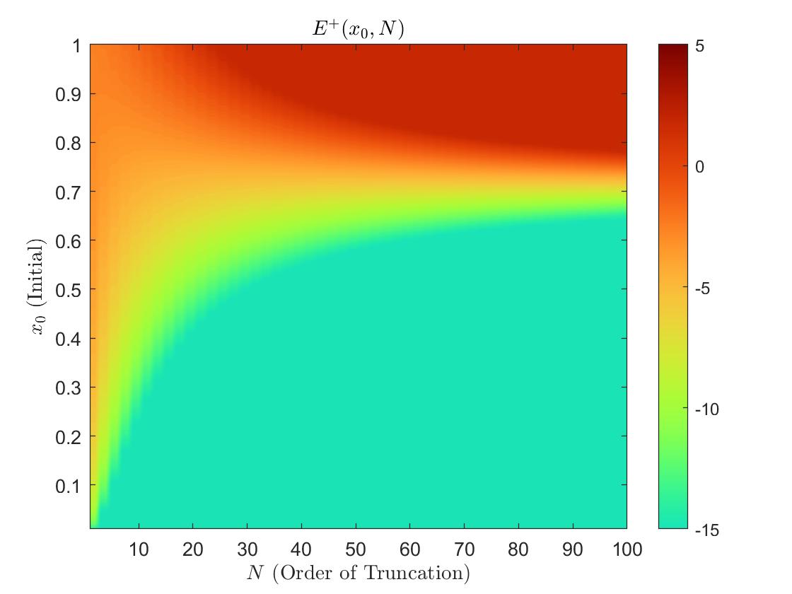
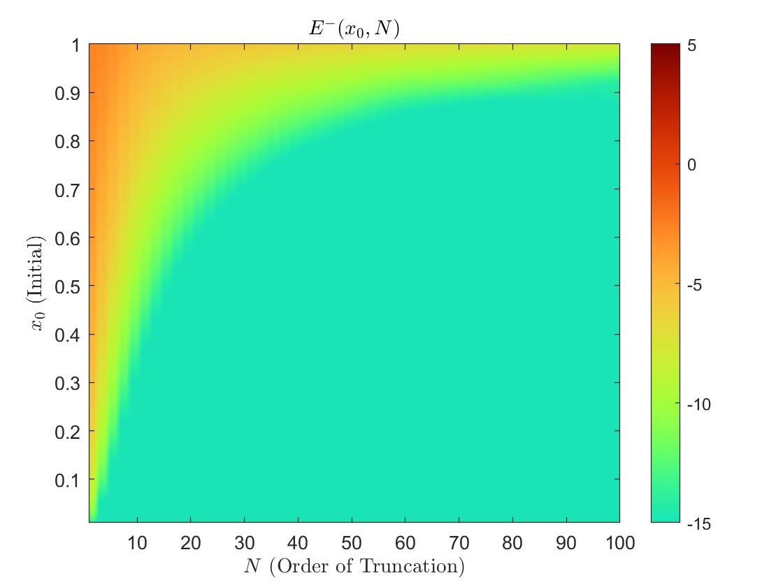
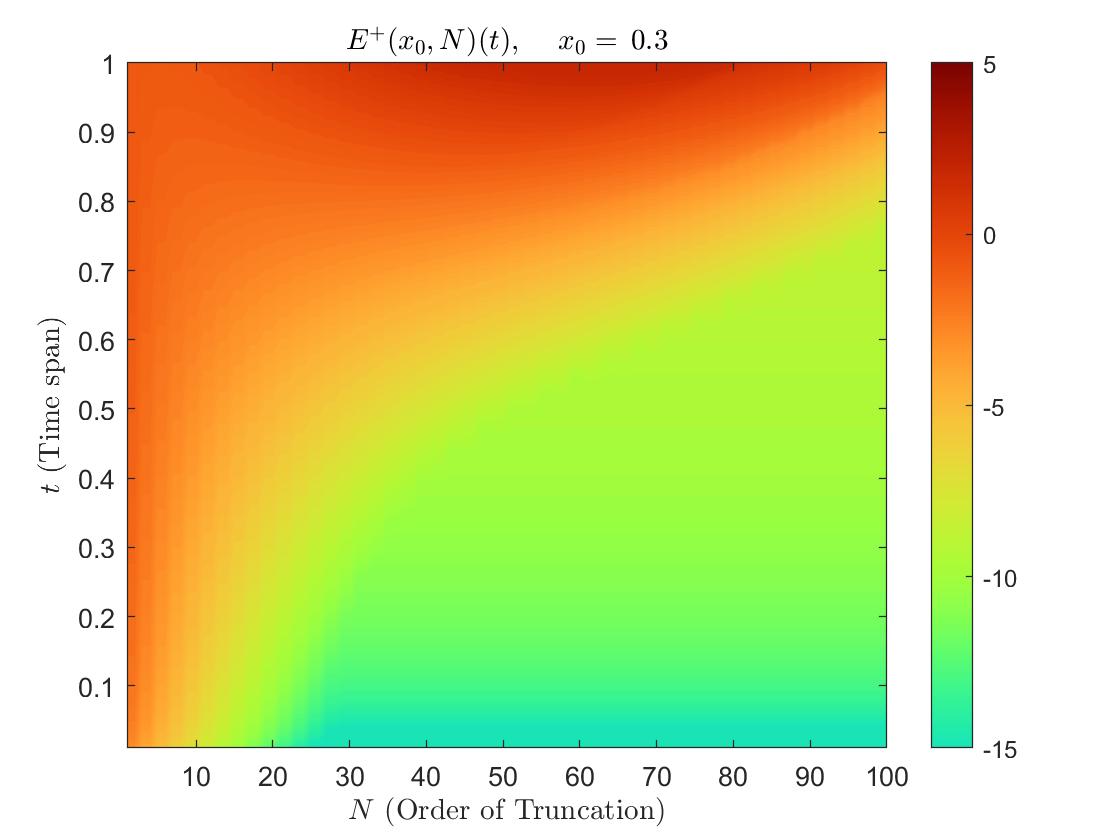
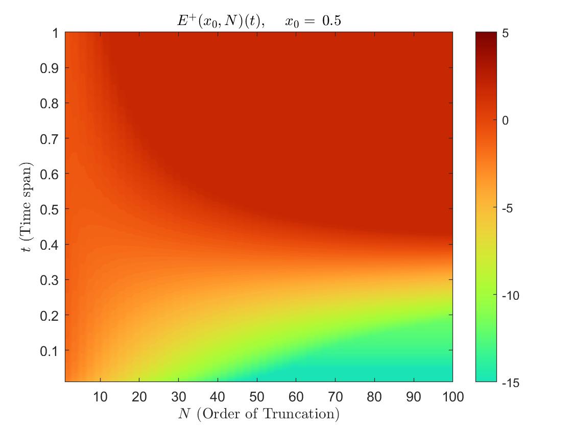
with $y_{k,N}^{\pm}(0)=x_{0}^{k}$ for $1\leq k\leq N$. For a given initial condition $x_{0}>0$, the truncation order $N\geq 1$, and time range $T^{*}>0$, let us denote the maximal (worst) approximation error between $y_{1,N}^{\pm}$ and the true solution $x^{\pm}$ during the time interval $[0,T^{*}]$ by

$$e_{\pm}(x_{0},N)=\sup_{0\leq t\leq T^{*}_{\pm}}\left|y_{1,N}^{\pm}(t)-x^{\pm}(t)\right|,$$

where

$$T^{*}_{+}=\max\left\{\frac{e-1}{2e-1}\left(\ln|x_{0}|^{-1}-1\right),0.1\right\}\ \ {\rm and}\ \ T^{*}_{-}=10.$$

Figure 4.1 shows the maximal approximation error

$$E^{\pm}(x_{0},N)=\log\min\left\{\max\left\{e_{\pm}(x_{0},N),10^{-15}\right\},10^{5}\right\}$$

in the logarithmic scale. We observe that for the stable dynamical system (4.1) with negative sign, the state variable $y_{1,N}^{-}$ for truncation orders $1\leq N\leq 100$ approximates the true solution $x^{-}$ quite well during the 10 seconds time interval for all initials $0<x_{0}<1$, while for the unstable dynamical system (4.1) with positive sign, the state variable $y_{1,N}^{+}$ for truncation orders $1\leq N\leq 100$ approximates the true solution $x^{+}$ quickly during time interval $[0,T^{*}_{+}]$ for all initials $0<x_{0}<0.7$. This validates the conclusions in Theorems 3.1 and 3.4 about exponential convergence when the initial is not far away from the origin. As expected from the requirements (3.1) and (3.4) in Theorems 3.1 and 3.4, the state variable $y^{+}_{1,N},1\leq N\leq 100$, does not provide good approximation to the true solution $x^{+}$ even over time interval $[0,0.1]$ when the initial is far away from the origin, e.g., when $x_{0}>0.8$.

(a)

(b)

Figure 4.1: Plotted are maximal approximation error $E^{\pm}(x_{0},N),1\leq N\leq 100,0\leq x_{0}\leq 1$ in the logarithmic scale between the first block $y_{1,N}^{\pm}$ of the finite section scheme (4.3) and the true solution $x^{\pm}$ of the dynamical system (4.1) with positive sign (left) and negative sign (right) during the time period $[0,T^{*}_{\pm}]$.

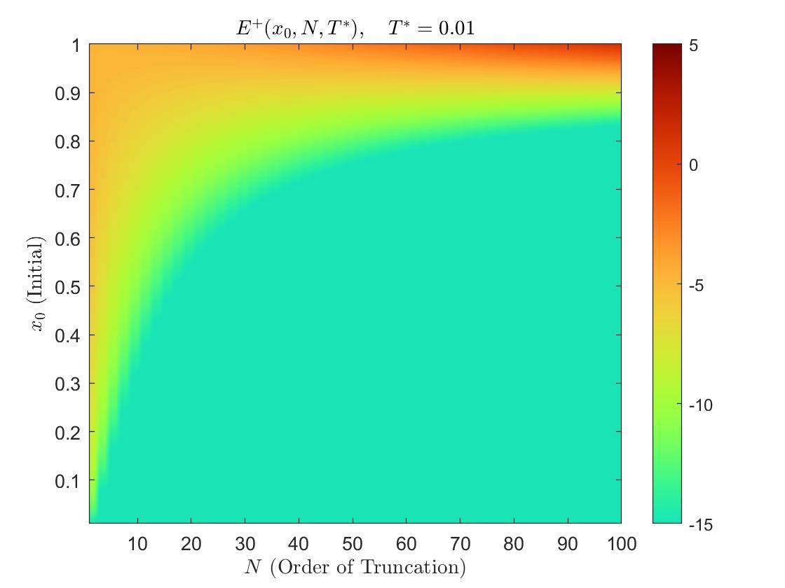
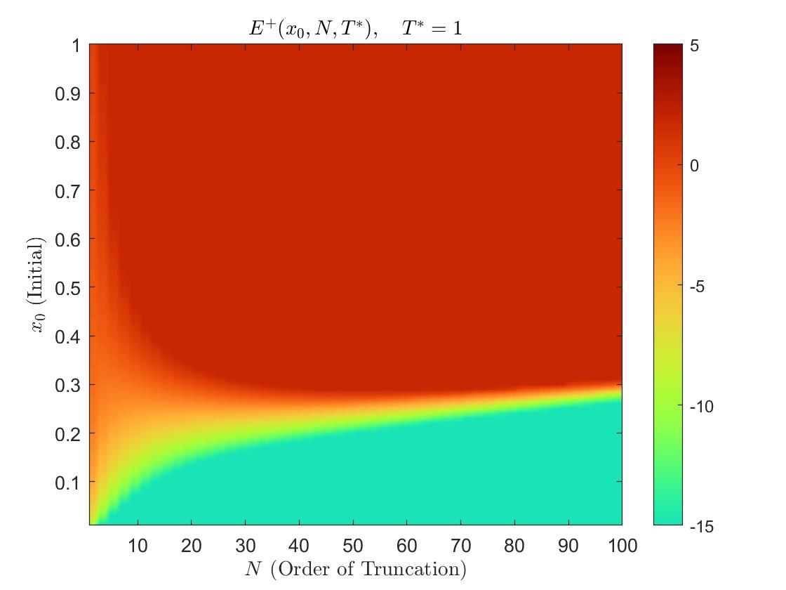
We conduct further numerical simulations on the convergence rate for different time intervals $[0,T^{*}]$ and initials $x_{0}$; see Figure 4.2. The top plots in Figure 4.2 are maximal approximation error

$$E^{+}(x_{0},N,T^{*})=\log\min\left\{\max\left\{e_{+}(x_{0},N,T^{*}),10^{-15}\right\},10^{5}\right\}$$

on time period $[0,T^{*}]$ in the logarithmic scale for different time ranges $T^{*}$, where the convergence region, i.e., $\log E^{+}(x_{0},N,T^{*})\leq-15$, is marked by the green color. As expected from (3.2) in Theorem 3.1, increasing the convergence range $[0,T^{*}]$ results in smaller initial range $[0,x_{0}]$. In particular, when we increase $T^{*}$ from $0.01$ to $0.10$ and then to $1.00$, the maximal initial condition $x_{0}$ decreases from $0.8423$ to $0.6722$ and then to $0.2348$, while the theoretical bound in (3.2) for the initial condition $x_{0}$ are $0.3582,0.2841$, and $0.0401$, respectively. The plots in the bottom of Figure 4.2 illustrate the approximation error

$$E^{+}(x_{0},N,t)=\log\min\left\{\max\left\{\left|y_{1,N}^{+}(t)-x^{+}(t)\right|,10^{-15}\right\},10^{5}\right\}$$

for $\ 0\leq t\leq 1$, in the logarithmic scale for various initials $x_{0}$. We notice that increasing the initial $x_{0}$ leads to the shrinkage of the convergence region marked by the green color, or equivalently, the time range for the convergence gets smaller when large initials are selected. This asserts that the finite-section scheme (4.3) of the Carleman linearization should not be utilized to approximate the original nonlinear dynamical system (4.1) with positive sign over long time intervals if the original nonlinear system is unstable.

(a)

(b)

(c)

(d)

Figure 4.2: Plotted on the top are maximal approximation error $E^{+}(x_{0},N,T^{*}),1\leq N\leq 100,0\leq x_{0}\leq 1,$ in the logarithmic scale with $T^{*}$ taking value $0.01$ (top left) and $1$ (top right) respectively. Plotted on the bottom are approximation error $E^{+}(x_{0},N)(t),1\leq N\leq 100,0\leq t\leq 1$ in the logarithmic scale for the initial $x_{0}=0.3$ and $0.5$ respectively.

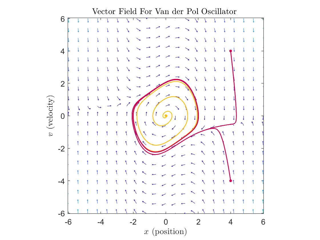
4.2 Carleman linearization of Van der Pol oscillator

In this part, we consider Carleman linearization of the Van der Pol oscillator whose dynamics can be described by a dynamical system of polynomial type

(4.4) $$\ddot{x}-\mu(1-x^{2})\dot{x}+x=0,$$

where $x$ stands for position and $\mu$ is an indicator parameter for non-linearity of the model. Using the state vector ${\bf x}=[x_{1},x_{2}]^{T}=[x,\dot{x}]^{T}$, this second-order system can be represented in the canonical form (1.1) as

(4.5) $$\dot{\bf x}=\left[\begin{array}[]{c}x_{2}\\ -x_{1}+\mu(1-x_{1}^{2})x_{2}\end{array}\right]=\left[\begin{array}[]{c}0\\ -1\end{array}\right]{\bf x}_{{\bf e}_{1}}+\left[\begin{array}[]{c}1\\ \mu\end{array}\right]{\bf x}_{{\bf e}_{2}}+\left[\begin{array}[]{c}0\\ -\mu\end{array}\right]{\bf x}_{2{\bf e}_{1}+{\bf e_{2}}},$$

where ${\bf e}_{1}=[1,0]^{T}$ and ${\bf e}_{2}=[0,1]^{T}$; see Figure 4.3 for the corresponding vector field. One may verify that the Van der Pol oscillator (4.5) satisfies Assumption 2.1 with $d=2,R>0$, and $D_{0}=\max\left\{(2+\mu)R,\mu R^{3}\right\}$. By utilizing the new state variables ${\bf z}_{k}=[x_{1}^{k},x_{1}^{k-1}x_{2},\ldots,x_{2}^{k}]^{T}$ for every $k\geq 1$ and looking at the sub-blocks of the state matrix (2.12), it turns out that ${\bf A}_{k,l}$ for all $1\leq k\leq l$ will be zero matrices of size $(k+1)\times(l+1)$ except for

$${\bf A}_{k,k}=\left[\begin{array}[]{ccccccccc}0&k&\\ -1&\mu&k-1&\\ &\ddots&\ddots&\ddots\\ &&\ddots&\ddots&\ddots\\ &&&\ddots&\ddots&\ddots\\ &&&&-k+1&(k-1)\mu&1\\ &&&&&-k&k\mu\end{array}\right]$$

and

$${\bf A}_{k,k+2}=\left[\begin{array}[]{ccccccccc}0&&&&0&0\\ &-\mu&&&\vdots&\vdots\\ &&\ddots&&\vdots&\vdots\\ &&&-k\mu&0&0\end{array}\right].$$

Therefore, the Carleman linearization of the Van der Pol oscillator is given by

(4.6) $$\left[\begin{array}[]{c}\dot{\bf z}_{1}\\ \dot{\bf z}_{2}\\ \vdots\end{array}\right]=\left[\begin{array}[]{cccccccccc}{\bf A}_{1,1}&{\bf 0}&{\bf A}_{1,3}&\\ &{\bf A}_{2,2}&{\bf 0}&{\bf A}_{2,4}&\\ &&\ddots&\ddots&\ddots&\\ \end{array}\right]\left[\begin{array}[]{c}{\bf z}_{1}\\ {\bf z}_{2}\\ \vdots\end{array}\right]$$

and its corresponding finite-section scheme of order $N$ is given by

(4.7) $$\left[\begin{array}[]{c}\dot{\bf y}_{1,N}\\ \dot{\bf y}_{2,N}\\ \vdots\\ \vdots\\ \dot{\bf y}_{N-1,N}\\ \dot{\bf y}_{N,N}\\ \end{array}\right]=\left[\begin{array}[]{cccccccccc}{\bf A}_{1,1}&{\bf 0}&{\bf A}_{1,3}&\\ &{\bf A}_{2,2}&{\bf 0}&{\bf A}_{2,4}&\\ &&\ddots&\ddots&\ddots&\\ &&&\ddots&\ddots&\\ &&&&{\bf A}_{N-1,N-1}&{\bf 0}\\ &&&&&{\bf A}_{N,N}\\ \end{array}\right]\left[\begin{array}[]{c}{\bf y}_{1,N}\\ {\bf y}_{2,N}\\ \vdots\\ \vdots\\ {\bf y}_{N-1,N}\\ {\bf y}_{N,N}\end{array}\right]$$

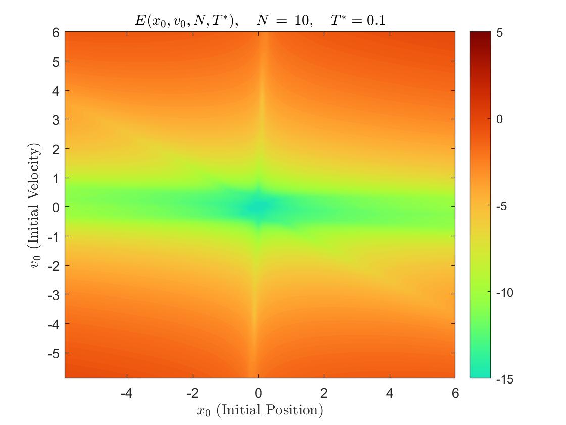
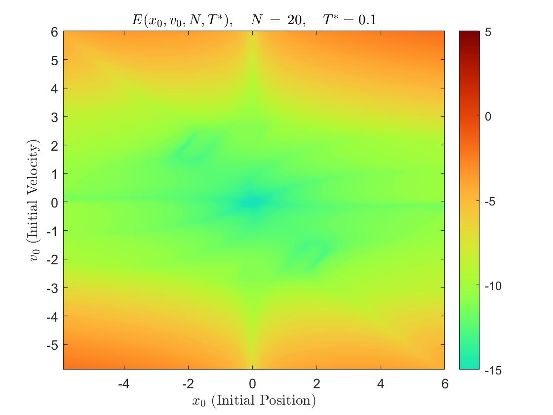
with initial ${\bf y}_{k,N}(0)=[x_{0}^{k},x_{0}^{k-1}v_{0},\ldots,x_{0}v_{0}^{k-1},v_{0}^{k}]^{T}$, where $x_{0}$ and $v_{0}$ are the initial position and velocity at time 0.

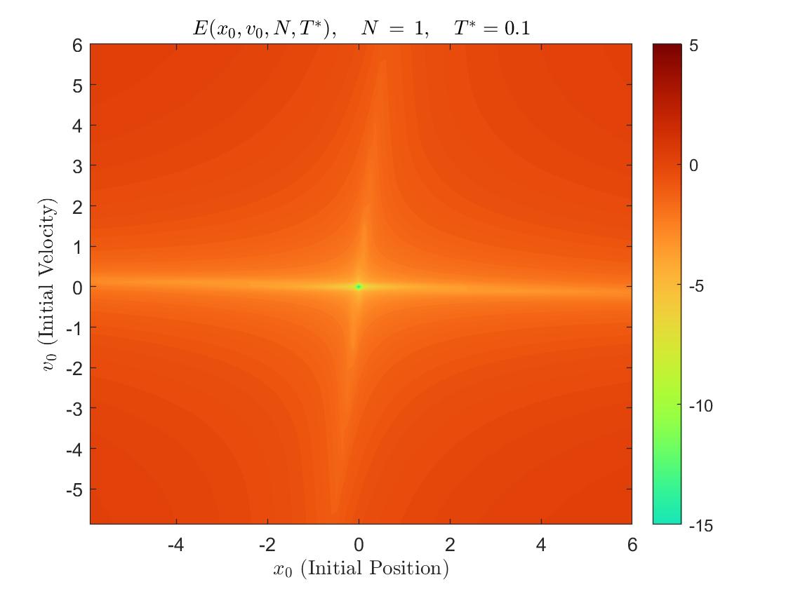
Let us define the maximal (worst) approximation error of the finite section scheme (4.7) on the time interval $[0,T^{*}]$ in the logarithmic scale by

$$E(x_{0},v_{0},N,T^{*})=\log\min\left\{\max\left\{\sup_{0\leq t\leq T^{*}}\left\|{\bf y}_{1,N}(t)-[x(t),x^{\prime}(t)]^{T}\right\|_{\infty},10^{-15}\right\},10^{5}\right\}$$

for $N\geq 1$, where $x(t)$ is the solution of the Van der Pol oscillator (4.4) with initial position $x_{0}$ and velocity $v_{0}$. We verify the approximation properties of the first block ${\bf y}_{1,N}(t)$ of the finite-section approximation (4.7) with respect to the true solution $[x(t),\dot{x}(t)]^{T}$ over a fixed time period $[0,T^{*}]$ for different values of the truncation order $N$. As expected from the exponential convergence results in Theorem 3.1, the convergence region of the initial $[x_{0},v_{0}]^{T}$ is larger for bigger truncation orders. Figure 4.3 shows the maximal approximation error $E(x_{0},v_{0},N,T^{*})$ for the range of initial conditions $-6\leq x_{0},v_{0}\leq 6$. As observed from the simulations, the convergence region for the traditional first-order linearization approach, i.e., when $N=1$, is much smaller (almost negligible) than the one for the finite-section approximation with large truncation orders, e.g., $N=10$ or $20$, which is depicted in Figure 4.3. These simulations assert that Carleman linearization of nonlinear system (1.1) can tightly approximate the original system over larger regions and longer time intervals with respect to the conventional first-order linearization approach.

(a)

(b)

(c)

(d)

Figure 4.3: Plotted on the top left is the vector field and limit cycle representation of the Van der Pol oscillator (4.5) with $\mu=0.5$. On the top right, bottom left and bottom right are the maximal approximation error $E(x_{0},v_{0},N,T^{*})$ in the logarithmic scale, where $T^{*}=0.1,\mu=0.5$ and the truncation order $N=1,10,20$ respectively.

5 Technical proofs of the main theorems

In this section, we prove Theorems 3.1 and 3.5.

5.1 Proof of Theorem 3.1

For two countable index sets $X$ and $Y$, let $\ell^{p}(X)$ be the space of all $p$-summable sequences ${\bf u}=[u(i)]_{i\in X}$ with norm denoted by $\|{\bf u}\|_{\ell^{p}(X)}$, and ${\mathcal{S}}(X,Y)$ and ${\mathcal{B}}_{p}(X,Y),1\leq p\leq\infty$, be Banach spaces of matrices ${\bf C}=[C(i,j)]_{i\in X,j\in Y}$ with the norm defined by

(5.1) $$\|{\bf C}\|_{{\mathcal{S}}(X,Y)}:=\max\left\{\sup_{i\in X}\sum_{j\in Y}|C(i,j)|,\ \sup_{j\in Y}\sum_{i\in X}|C(i,j)|\right\}$$

and

(5.2) $$\|{\bf C}\|_{{\mathcal{B}}_{p}(X,Y)}:=\sup_{{\bf u}\neq{\bf 0}}\frac{\|{\bf C}{\bf u}\|_{\ell^{p}(X)}}{\|{\bf u}\|_{\ell^{p}(Y)}},$$

respectively. The norms in (5.1) and (5.2) are known as the Schur norm and the operator norm from $\ell^{p}(Y)$ to $\ell^{p}(X)$. By direct computation, one may verify that $\|{\bf C}\|_{{\mathcal{B}}_{1}(X,Y)}=\sup_{j\in Y}\sum_{i\in X}|C(i,j)|$ and $\|{\bf C}\|_{{\mathcal{B}}_{\infty}(X,Y)}=\sup_{i\in X}\sum_{j\in Y}|C(i,j)|$. This together with the interpolation theory ([7]) yields

(5.3) $$\|{\bf C}\|_{{\mathcal{S}}(X,Y)}=\sup_{1\leq p\leq\infty}\|{\bf C}\|_{{\mathcal{B}}_{p}(X,Y)}.$$

For countable index sets $X,Y,Z$ and matrices ${\bf C}\in{\mathcal{S}}(X,Y)$ and ${\bf D}\in{\mathcal{S}}(Y,Z)$, one has

(5.4) $$\|{\bf C}{\bf D}\|_{{\mathcal{S}}(X,Z)} \hskip-0.72229pt= \hskip-0.72229pt\sup_{1\leq p\leq\infty}\|{\bf C}{\bf D}\|_{{\mathcal{B}}_{p}(X,Z)}$$

$$\hskip-0.72229pt\leq \hskip-0.72229pt\sup_{1\leq p\leq\infty}\|{\bf C}\|_{{\mathcal{B}}_{p}(X,Y)}\|{\bf D}\|_{{\mathcal{B}}_{p}(Y,Z)}\leq\|{\bf C}\|_{{\mathcal{S}}(X,Y)}\|{\bf D}\|_{{\mathcal{S}}(Y,Z)}.$$

Then, for any countable set $X$, ${\mathcal{S}}(X,X)$ is a Banach subalgebra of ${\mathcal{B}}_{p}(X,X),1\leq p\leq\infty$ which is known as the Schur algebra, see [11, 22, 26, 28, 29] for the inverse-closed property of Banach algebra of infinite matrices.

To prove Theorem 3.1, we need the following Schur norm estimates for block matrices ${\bf A}_{k,l}(t)$ of the time-varying state matrices ${\bf A}(t)$ in (2.12).

Lemma 5.1.

Let ${\bf f}(t,{\bf x})$ be as in Theorem 3.1, and ${\bf A}_{k,l}(t),k,l\geq 1$ be defined by (2.9). Then

(5.5) $${\bf A}_{k,l}(t)=0\ \ {\rm if}\ \ 1\leq l<k,$$

and

(5.6) $$\sup_{t\geq t_{0}}\|{\bf A}_{k,l}(t)\|_{{\mathcal{S}}({\mathbb{Z}}^{d}_{k},{\mathbb{Z}}^{d}_{l})}\leq D_{0}kR^{k-l-1}\ \ {\rm if}\ \ 1\leq k\leq l.$$

Proof 5.2.

First we prove (5.5). By (2.5) and (2.9), the proof of the conclusion (5.5) reduces to establishing ${\boldsymbol{\beta}}-{\boldsymbol{\alpha}}+{\bf e}_{j}\not\in{\mathbb{Z}}_{+}^{d}\backslash\{0\},\ 1\leq j\leq d$, for all ${\boldsymbol{\alpha}}\in{\mathbb{Z}}^{d}_{k}$ and ${\boldsymbol{\beta}}\in{\mathbb{Z}}_{l}^{d}$ with $l<k$. Suppose, on the contrary, that ${\boldsymbol{\beta}}-{\boldsymbol{\alpha}}+{\bf e}_{j}\in{\mathbb{Z}}_{+}^{d}\backslash\{0\}$ for some $1\leq j\leq d$. Then $l+1=|{\boldsymbol{\beta}}+{\bf e}_{j}|=|{\boldsymbol{\alpha}}+({\boldsymbol{\beta}}-{\boldsymbol{\alpha}}+{\bf e}_{j})|>|{\boldsymbol{\alpha}}|=k$, which contradicts to the assumption that $1\leq l<k$.

Next we prove (5.6). For ${\boldsymbol{\alpha}}\in{\mathbb{Z}}^{d}_{+}$, we write ${\boldsymbol{\alpha}}=[\alpha_{1},\ldots,\alpha_{d}]^{T}$. For integers $k$ and $l$ with $k\leq l$ and $t\geq t_{0}$,

(5.7) $$\hskip-0.72229pt\max\left\{\sup_{{\boldsymbol{\alpha}}\in{\mathbb{Z}}_{k}^{d}}\sum_{{\boldsymbol{\beta}}\in{\mathbb{Z}}_{l}^{d}}\left|\sum_{j=1}^{d}\alpha_{j}f_{j,\boldsymbol{\beta}-\boldsymbol{\alpha}+{\bf e}_{j}}(t)\right|,\ \sup_{{\boldsymbol{\beta}}\in{\mathbb{Z}}_{l}^{d}}\sum_{{\boldsymbol{\alpha}}\in{\mathbb{Z}}_{k}^{d}}\left|\sum_{j=1}^{d}\alpha_{j}f_{j,\boldsymbol{\beta}-\boldsymbol{\alpha}+{\bf e}_{j}}(t)\right|\right\}$$

$$\hskip-0.72229pt\leq \hskip-0.72229ptk\max\left\{\sup_{{\boldsymbol{\alpha}}\in{\mathbb{Z}}_{k}^{d}}\sum_{{\boldsymbol{\beta}}\in{\mathbb{Z}}_{l}^{d}}\sum_{j=1}^{d}\left|f_{j,\boldsymbol{\beta}-\boldsymbol{\alpha}+{\bf e}_{j}}(t)\right|,\ \sup_{{\boldsymbol{\beta}}\in{\mathbb{Z}}_{l}^{d}}\sum_{{\boldsymbol{\alpha}}\in{\mathbb{Z}}_{k}^{d}}\sum_{j=1}^{d}|f_{j,\boldsymbol{\beta}-\boldsymbol{\alpha}+{\bf e}_{j}}(t)|\right\}$$

$$\hskip-0.72229pt\leq \hskip-0.72229ptk\sum_{j=1}^{d}\sum_{{\boldsymbol{\gamma}}\in{\mathbb{Z}}^{d}_{l-k+1}}\left|f_{j,\boldsymbol{\gamma}}(t)\right|\leq D_{0}kR^{k-l-1},$$

where the first inequality holds as $0\leq\alpha_{j}\leq|{\boldsymbol{\alpha}}|=k$ for all $1\leq j\leq d$, the second inequality follows from (2.5) and the observation that $|{\boldsymbol{\beta}}-{\boldsymbol{\alpha}}+{\bf e}_{j}|=|{\boldsymbol{\beta}}|-|{\boldsymbol{\alpha}}|+1=k-l+1$ when ${\boldsymbol{\beta}}-{\boldsymbol{\alpha}}+{\bf e}_{j}\in{\mathbb{Z}}_{+}^{d}$, and the last inequality is true by the assumption (2.2). Taking supernum over $t\geq t_{0}$ in (5.7) proves (5.6).

To prove Theorem 3.1, we need the following local bound estimate for the solution ${\bf x}(t)$ of the nonlinear dynamical system (1.1).

Lemma 5.3.

Let ${\bf f}(t,{\bf x})$ be as in Theorem 3.1 and ${\bf x}(t),t\geq t_{0}$, be the solution of the nonlinear dynamical system (1.1). If the nonzero initial ${\bf x}_{0}$ satisfies (3.1), then (3.7) holds.

Proof 5.4.

Let

(5.8) $$t_{1}^{*}=\sup\big{\{}t,\ \|{\bf x}(s)\|_{\infty}\leq M_{0}\ \ {\rm for\ all}\ \ t_{0}\leq s\leq t\big{\}}.$$

By the continuity of the solution ${\bf x}(t)$ of the nonlinear system (1.1) and the assumption (3.1) on the initial ${\bf x}_{0}$ that $\|{\bf x}(t_{0})\|_{\infty}=\|{\bf x}_{0}\|_{\infty}<M_{0}$, we have that $t_{1}^{*}>t_{0}$.

The conclusion (3.7) is obvious if $t_{1}^{*}=+\infty$. Then it remains to consider the case that $t_{0}<t_{1}<\infty$. In this case, we obtain from the continuity of ${\bf x}(t),t\geq t_{0}$, that

(5.9) $$\|{\bf x}(t_{1}^{*})\|_{\infty}=M_{0}.$$

Integrating the nonlinear dynamical system (1.1) yields

$${\bf x}(t)={\bf x}_{0}+\int_{t_{0}}^{t}{\bf f}(s,{\bf x}(s))ds={\bf x}_{0}+\int_{t_{0}}^{t}\sum_{\boldsymbol{\alpha}\in{\bf Z}_{+}^{d}\backslash\{0\}}f_{\boldsymbol{\alpha}}(s)({\bf x}(s))^{\boldsymbol{\alpha}}ds,$$

where the last equality follows from the Maclaurin expansion (2.1) of the function ${\bf f}(t,{\bf x})$. Hence for $t_{0}\leq t\leq t_{1}^{*}$, we have

(5.10) $$\|{\bf x}(t)\|_{\infty} \hskip-0.72229pt\leq \hskip-0.72229pt\|{\bf x}_{0}\|_{\infty}+\int_{t_{0}}^{t}\sum_{k=1}^{\infty}\left(\sum_{j=1}^{d}\sum_{{\boldsymbol{\alpha}}\in{\mathbb{Z}}_{k}^{d}}|f_{j,\boldsymbol{\alpha}}(s)|\right)\|{\bf x}(s)\|_{\infty}^{k}ds$$

$$\hskip-0.72229pt\leq \hskip-0.72229pt\|{\bf x}_{0}\|_{\infty}+D_{0}\int_{t_{0}}^{t}\sum_{k=1}^{\infty}R^{-k}\|{\bf x}(s)\|_{\infty}^{k}ds\leq\|{\bf x}_{0}\|_{\infty}+\frac{D_{0}}{R-M_{0}}\int_{t_{0}}^{t}\|{\bf x}(s)\|ds,$$

where the second estimate follows from (2.2) and the last inequality holds by (5.8). Let us set

$$u(t)=\int_{t_{0}}^{t}\|{\bf x}(s)\|_{\infty}ds-\frac{(R-M_{0})\|{\bf x}_{0}\|_{\infty}}{D_{0}}\left(e^{D_{0}(t-t_{0})/(R-M_{0})}-1\right),\ \ t_{0}\leq t\leq t_{1}^{*}.$$

Then, $u(t_{0})=0$ and

$$\hskip-0.72229pt\frac{d\big{(}e^{-D_{0}(t-t_{0})/(R-M_{0})}u(t)\big{)}}{dt}=e^{-D_{0}(t-t_{0})/(R-M_{0})}\left(-\frac{D_{0}}{R-M_{0}}u(t)+\frac{du(t)}{dt}\right)$$

$$\hskip-0.72229pt\leq \hskip-0.72229pte^{-D_{0}(t-t_{0})/(R-M_{0})}\left(\|{\bf x}(t)\|_{\infty}-\|{\bf x}_{0}\|_{\infty}-\frac{D_{0}}{R-M_{0}}\int_{t_{0}}^{t}\|{\bf x}(s)\|_{\infty}ds\right)\leq 0,$$

where the last inequality follows from (5.10). This implies that $u(t)\leq 0$ for all $t_{0}\leq t\leq t_{1}^{*}$, and hence

(5.11) $$\int_{t_{0}}^{t}\|{\bf x}(s)\|_{\infty}ds\leq\frac{(R-M_{0})\|{\bf x}_{0}\|_{\infty}}{D_{0}}\left(e^{D_{0}(t-t_{0})/(R-M_{0})}-1\right)\ {\rm for\ all}\ t_{0}\leq t\leq t_{1}^{*}.$$

Substituting the above estimate into (5.10), we obtain

(5.12) $$\|{\bf x}(t)\|_{\infty}\leq\|{\bf x}_{0}\|_{\infty}e^{D_{0}(t-t_{0})/(R-M_{0})},\ t_{0}\leq t\leq t_{1}^{*}.$$

Combining (3.1), (3.6), (5.9) and (5.12) proves that

$$t_{1}^{*}\geq t_{0}+\frac{R-M_{0}}{D_{0}}\ln\frac{M_{0}}{\|{\bf x}_{0}\|_{\infty}}\geq t_{0}+T^{*}.$$

This together with (5.8) proves (3.7).

To prove Theorem 3.1, we need a kernel estimate for the solution of an ordinary differential equation with the bounded state matrix in the Schur norm.

Lemma 5.5.

Let $1\leq p\leq\infty$, $X$ be a countable index set, the vector-valued function ${\bf w}(t),t\geq t_{0}$, be locally bounded in $\ell^{p}(X)$,

(5.13) $$\sup_{t_{0}\leq t\leq t_{1}}\|{\bf w}(t)\|_{\ell^{p}(X)}<\infty\ {\rm for\ all}\ t_{1}<\infty,$$

and let the matrix-valued function ${\bf B}(t),t\geq t_{0}$, be bounded in the Schur algebra ${\mathcal{S}}(X,X)$,

(5.14) $$\|{\bf B}\|_{\infty,{\mathcal{S}}(X,X)}:=\sup_{t\geq t_{0}}\|{\bf B}(t)\|_{{\mathcal{S}}(X,X)}<\infty.$$

Then the locally bounded solution of the ordinary different equation

(5.15) $$\dot{\bf z}(t)={\bf B}(t){\bf z}(t)+{\bf w}(t),\ t\geq t_{0}\ \ {\rm with\ zero\ initial}\ \ {\bf z}(t_{0})={\bf 0}$$

in $\ell^{p}(X)$ has the following expression,

(5.16) $${\bf z}(t)=\int_{t_{0}}^{t}{\bf K}(t,s){\bf w}(s)ds$$

where the integral kernel ${\bf K}$ satisfies

(5.17) $$\|{\bf K}(t,s)\|_{{\mathcal{S}}(X,X)}\leq\exp\big{(}\|{\bf B}\|_{\infty,{\mathcal{S}}(X,X)}(t-s)\big{)}\ \ {\rm for\ all}\ \ t\geq s\geq t_{0}.$$

Proof 5.6.

Define integral kernels ${\bf T}_{n}$ and ${\bf S}_{n},n\geq 0$, inductively by

$${\bf T}_{n}(t,s):=\int_{s}^{t}{\bf T}_{n-1}(t,u){\bf B}(s)du\ \ {\rm and}\ \ {\bf S}_{n}(t,s):=\int_{s}^{t}{\bf T}_{n-1}(t,u)du,\ n\geq 1,$$

with the initial integral kernels ${\bf T}_{0}$ and ${\bf S}_{0}$ given by ${\bf T}_{0}(t,s):={\bf B}(s)$ and ${\bf S}_{0}(t,s):={\bf I},\ \ t\geq s\geq t_{0}.$ By induction, we may verify that

(5.18) $$\|{\bf T}_{n}(t,s)\|_{{\mathcal{S}}(X,X)}\leq\|{\bf B}\|_{\infty,{\mathcal{S}}(X,X)}^{n+1}\frac{(t-s)^{n}}{n!},$$

and

(5.19) $$\|{\bf S}_{n}(t,s)\|_{{\mathcal{S}}(X,X)}\leq\|{\bf B}\|_{\infty,{\mathcal{S}}(X,X)}^{n}\frac{(t-s)^{n}}{n!},\ t\geq s\geq t_{0},$$

for all $n\geq 0$. Define

(5.20) $${\bf K}(t,s):=\sum_{k=0}^{\infty}{\bf S}_{k}(t,s),\ \ t\geq s\geq t_{0}.$$

Then we get from (5.19) that

(5.21) $$\|{\bf K}(t,s)\|_{{\mathcal{S}}(X,X)}\leq\sum_{n=0}^{\infty}\|{\bf S}_{k}(t,s)\|_{{\mathcal{S}}(X,X)}\sum_{k=0}^{\infty}\|{\bf B}\|_{\infty,{\mathcal{S}}(X,X)}^{k}\frac{(t-s)^{k}}{k!}$$

for all $t\geq s\geq t_{0}$. This proves (5.17).

Now it remains to prove (5.16) with the integral kernel ${\bf K}$ given in (5.20). Integrating both sides of the ordinary differential equation (5.15) gives

(5.22) $${\bf z}(t)=\int_{t_{0}}^{t}{\bf B}(s){\bf z}(s)ds+\int_{t_{0}}^{t}{\bf w}(s)ds,\ t\geq t_{0}.$$

Applying (5.22) for $n$ times, we obtain

(5.23) $${\bf z}(t) \hskip-0.72229pt= \hskip-0.72229pt\int_{t_{0}}^{t}{\bf B}(u)\left(\int_{t_{0}}^{u}{\bf B}(s){\bf z}(s)ds+\int_{t_{0}}^{u}{\bf w}(s)ds\right)du+\int_{t_{0}}^{t}{\bf w}(s)ds$$

$$\hskip-0.72229pt= \hskip-0.72229pt\int_{t_{0}}^{t}{\bf T}_{1}(t,s){\bf z}(s)ds+\int_{t_{0}}^{t}\left(\sum_{k=0}^{1}{\bf S}_{k}(t,s\right){\bf w}(s)ds=\cdots$$

$$\hskip-0.72229pt= \hskip-0.72229pt\int_{t_{0}}^{t}{\bf T}_{n}(t,s){\bf z}(s)ds+\int_{t_{0}}^{t}\left(\sum_{k=0}^{n}{\bf S}_{k}(t,s)\right){\bf w}(s)ds,\ t\geq t_{0}.$$

Using the local boundedness of ${\bf z}(t),t\geq t_{0}$, in $\ell^{p}(X)$ and applying (5.3) and (5.18), we have

(5.24) $$\hskip-0.72229pt\Big{\|}\int_{t_{0}}^{t}{\bf T}_{n}(t,s){\bf z}(s)ds\Big{\|}_{\ell^{p}(X)}\leq\int_{t_{0}}^{t}\|{\bf T}_{n}(t,s)\|_{{\mathcal{S}}(X,X)}\|{\bf z}(s)\|_{\ell^{p}(X)}ds$$

$$\hskip-0.72229pt\leq \hskip-0.72229pt\frac{\|{\bf B}\|_{\infty,{\mathcal{S}}(X,X)}^{n+1}(t-t_{0})^{n}}{n!}\int_{t_{0}}^{t}\|{\bf z}(s)\|_{\ell^{p}(X)}ds\to 0\ \ {\rm as}\ \ n\to\infty.$$

Similarly, from (5.3), (5.13) and (5.19) we obtain

(5.25) $$\hskip-0.72229pt\Big{\|}\int_{t_{0}}^{t}{\bf K}(t,s){\bf w}(s)ds-\int_{t_{0}}^{t}\left(\sum_{k=0}^{n}{\bf S}_{k}(t,s)\right){\bf w}(s)ds\Big{\|}_{\ell^{p}(X)}$$

$$\hskip-0.72229pt\leq \hskip-0.72229pt\int_{t_{0}}^{t}\sum_{k=n+1}^{\infty}\|{\bf S}_{k}(t,s)\|_{{\mathcal{S}}(X,X)}\|{\bf w}(s)\|_{\ell^{p}(X)}ds$$

$$\hskip-0.72229pt\leq \hskip-0.72229pt\left(\sum_{k=n+1}^{\infty}\frac{\|{\bf B}\|_{\infty,{\mathcal{S}}(X,X)}^{k}(t-t_{0})^{k}}{k!}\right)\int_{t_{0}}^{t}\|{\bf w}(s)\|_{\ell^{p}(X)}ds\to 0\ \ {\rm as}\ \ n\to\infty.$$

Combining (5.23), (5.24) and (5.25) proves (5.16). This together with (5.21) completes the proof.

The final technical lemma used in our proof of Theorem 3.1 is as follows.

Lemma 5.7.

Let $D_{1}>0$ and $v_{k},1\leq k\leq N$, be nonnegative functions satisfying

(5.26) $$0\leq v_{k}(t)\leq D_{1}k\int_{t_{0}}^{t}e^{D_{1}k(t-s)}\left(\sum_{l=k+1}^{N}v_{l}(s)+1\right)ds,\ \ t\geq t_{0},$$

then

(5.27) $$v_{N-n}(t)+\cdots+v_{N}(t)+1\leq\frac{N^{n}}{n!}e^{D_{1}N(t-t_{0})},\ t\geq t_{0}$$

for all $0\leq n\leq N-2$.

Proof 5.8.

We prove (5.27) by induction on $n=0,1,\ldots,N-2$. Applying (5.26) with $k=N$, we have

$$v_{N}(t)+1\leq D_{1}N\int_{t_{0}}^{t}e^{D_{1}N(t-s)}ds+1=e^{D_{1}N(t-t_{0})},\ t\geq t_{0}.$$

This proves (5.27) for $n=0$.

Inductively we assume that the conclusion (5.27) for $0\leq n\leq N-2$. Applying (5.26) with $k$ replaced by $N-n-1$, we obtain from the inductive hypothesis that

$$v_{N-n-1}(t)+v_{N-n}(t)+\cdots+v_{N}(t)+1$$

$$\hskip-0.72229pt\leq \hskip-0.72229ptD_{1}(N-n-1)\int_{t_{0}}^{t}e^{D_{1}(N-n-1)(t-s)}\frac{N^{n}}{n!}e^{D_{1}N(s-t_{0})}ds+\frac{N^{n}}{n!}e^{D_{1}N(t-t_{0})}$$

$$\hskip-0.72229pt= \hskip-0.72229pt\frac{N^{n}(N-n-1)}{(n+1)!}\Big{(}e^{D_{1}N(t-t_{0})}-e^{D_{1}(N-n-1)(t-t_{0})}\Big{)}+\frac{N^{n}}{n!}e^{D_{1}N(t-t_{0})}$$

$$\hskip-0.72229pt\leq \hskip-0.72229pt\frac{N^{n+1}}{(n+1)!}e^{D_{1}N(t-t_{0})},$$

for all $t\geq t_{0}$. Therefore the inductive argument can proceed. This completes the inductive proof of the conclusion (5.27).

We finish this subsection with the proof of Theorem 3.1.

Proof 5.9.

Set $\boldsymbol{\eta}_{k,N}(t)={\bf y}_{k,N}(t)-{\bf z}_{k}(t),t\geq t_{0}$, for $1\leq k\leq N$ and $\|{\bf A}_{k,l}\|_{\infty,{\mathcal{S}}({\mathbb{Z}}_{k}^{d},{\mathbb{Z}}_{l}^{d})}=\sup_{t\geq t_{0}}\|{\bf A}_{k,l}(t)\|_{{\mathcal{S}}({\mathbb{Z}}_{k}^{d},{\mathbb{Z}}_{l}^{d})}$, $k,l\geq 1$. Then we obtain from (2.12) that

(5.28) $$\dot{\boldsymbol{\eta}}_{k,N}(t)={\bf A}_{k,k}(t)\boldsymbol{\eta}_{k,N}(t)+\sum_{l=k+1}^{N}{\bf A}_{k,l}(t)\boldsymbol{\eta}_{l,N}(t)-\sum_{l=N+1}^{\infty}{\bf A}_{k,l}(t){\bf z}_{l}(t)$$

with zero initial ${\bf\eta}_{k,N}(t_{0})={\bf 0},1\leq k\leq N$. Applying Lemma 5.5 with ${\bf B}(t)$ and ${\bf w}(t)$ replaced by ${\bf A}_{k,k}(t)$ and $\sum_{l=k+1}^{N}{\bf A}_{k,l}(t){\boldsymbol{\eta}}_{l,N}(t)-\sum_{l=N+1}^{\infty}{\bf A}_{k,l}(t){\bf z}_{l}(t)$ respectively, we can construct an integral kernel ${\bf K}_{k}(t,s),t,s\geq t_{0}$ such that

(5.29) $${\boldsymbol{\eta}}_{k,N}(t)=\int_{t_{0}}^{t}{\bf K}_{k}(t,s)\left(\sum_{l=k+1}^{N}{\bf A}_{k,l}(s){\boldsymbol{\eta}}_{l,N}(s)-\sum_{l=N+1}^{\infty}{\bf A}_{k,l}(s){\bf z}_{l}(s)\right)ds$$

and

(5.30) $$\|{\bf K}_{k}(t,s)\|_{{\mathcal{S}}({\mathbb{Z}}_{k}^{d},{\mathbb{Z}}_{k}^{d})}\leq\exp\left({\|{\bf A}_{k,k}\|_{\infty,{\mathcal{S}}({\mathbb{Z}}_{k}^{d},{\mathbb{Z}}_{k}^{d})}(t-s)}\right)$$

for $t\geq s\geq t_{0}$. By (5.3), (5.29), (5.30) and Lemmas 5.1 and 5.3, we obtain

(5.31) $$\|{\boldsymbol{\eta}}_{k,N}(t)\|_{\ell^{\infty}({\mathbb{Z}}^{d}_{k})} \hskip-0.72229pt\leq \hskip-0.72229pt\int_{t_{0}}^{t}e^{\|{\bf A}_{k,k}\|_{\infty,{\mathcal{S}}({\mathbb{Z}}_{k}^{d},{\mathbb{Z}}_{k}^{d})}(t-s)}\left(\sum_{l=k+1}^{N}\|{\bf A}_{k,l}(t)\|_{\infty,{\mathcal{S}}({\mathbb{Z}}_{k}^{d},{\mathbb{Z}}_{l}^{d})}\right.$$

$$\hskip-0.72229pt\left.\times~{}\|\boldsymbol{\eta}_{l,N}(s)\|_{\ell^{\infty}({\mathbb{Z}}^{d}_{l})}+\sum_{l=N+1}^{\infty}\|{\bf A}_{k,l}\|_{\infty,{\mathcal{S}}({\mathbb{Z}}_{k}^{d},{\mathbb{Z}}_{l}^{d})}\|{\bf z}_{l}(s)\|_{\ell^{\infty}({\mathbb{Z}}_{l}^{d})}\right)ds$$

$$\hskip-0.72229pt\leq \hskip-0.72229ptD_{0}k\sum_{l=k+1}^{N}R^{k-l-1}\int_{t_{0}}^{t}e^{D_{0}k(t-s)/R}\|\boldsymbol{\eta}_{l,N}(s)\|_{\ell^{\infty}({\mathbb{Z}}^{d}_{l})}ds$$

$$\hskip-0.72229pt+D_{0}k\int_{t_{0}}^{t}e^{D_{0}k(t-s)/R}\left(\sum_{l=N+1}^{\infty}R^{k-l-1}\|{\bf x}(s)\|_{\infty}^{l}\right)ds$$

$$\hskip-0.72229pt\leq \hskip-0.72229pt\frac{D_{0}k}{R}\sum_{l=k+1}^{N}R^{k-l}\int_{t_{0}}^{t}e^{D_{0}k(t-s)/R}\|\boldsymbol{\eta}_{l,N}(s)\|_{\infty}ds$$

$$\hskip-0.72229pt+\frac{D_{0}k}{R}\int_{t_{0}}^{t}e^{D_{0}k(t-s)/R}(R-M_{0})^{-1}R^{k-N}M_{0}^{N+1}ds$$

for all $t_{0}\leq t\leq t_{0}+T^{*}$ and $1\leq k\leq N$. Set

(5.32) $$v_{k}(t)=(R-M_{0})R^{N-k}M_{0}^{-N-1}\|\boldsymbol{\eta}_{k,N}(t)\|_{\infty},\ \ t_{0}\leq t\leq t_{0}+T^{*},$$

for $1\leq k\leq N$. Multiplying $(R-M_{0})R^{N-k}M_{0}^{-N-1}$ at both sizes of (5.31) yields

(5.33) $$v_{k}(t)\leq\frac{D_{0}k}{R}\int_{t_{0}}^{t}e^{D_{0}k(t-s)/R}\left(\sum_{l=k+1}^{N}v_{l}(s)+1\right)ds,\ \ 1\leq k\leq N.$$

Therefore

(5.34) $$v_{2}(t)+\cdots+v_{N}(t)+1\leq\frac{N^{N-2}}{(N-2)!}e^{D_{0}N(t-t_{0})/R},\ t_{0}\leq t\leq t_{0}+T^{*},$$

by Lemma 5.7. Applying (5.33) with $k=1$ and the estimate in (5.34), we obtain that

(5.35) $$v_{1}(t)\leq\frac{D_{0}}{R}\frac{N^{N-2}}{(N-2)!}\int_{t_{0}}^{t}e^{D_{0}(t-s)/R}e^{D_{0}N(s-t_{0})/R}ds\leq\frac{N^{N-2}}{(N-1)!}e^{D_{0}N(t-t_{0})/R}$$

hold for all $t\in[t_{0},t_{0}+T^{*}]$. Therefore

(5.36) $$\|{\bf y}_{1,N}(t)-{\bf x}(t)\|_{\infty} \hskip-0.72229pt= \hskip-0.72229pt\|{\boldsymbol{\eta}}_{1,N}(t)\|_{\infty}=\frac{RM_{0}}{R-M_{0}}\Big{(}\frac{M_{0}}{R}\Big{)}^{N}v_{1}(t)$$

$$\hskip-0.72229pt\leq \hskip-0.72229pt\frac{RM_{0}}{R-M_{0}}\frac{N^{N-1}}{N!}\left(\frac{M_{0}e^{D_{0}(t-t_{0})/R}}{R}\right)^{N}$$

$$\hskip-0.72229pt\leq \hskip-0.72229pt\frac{RM_{0}}{\sqrt{2\pi}(R-M_{0})}N^{-3/2}\left(\frac{eM_{0}}{R}e^{D_{0}(t-t_{0})/R}\right)^{N},\ \ t_{0}\leq t\leq t_{0}+T^{*},$$

where the last inequality follows from the Stiriling formula, $N!\geq\sqrt{2\pi}N^{N+1/2}e^{-N}$ for $N\geq 1$. This proves the exponential convergence in (3.5).

5.2 Proof of Theorem 3.5

To prove Theorem 3.5, we need the following Schur norm estimate for the block matrices ${\bf A}_{k,l}$ for all $k,l\geq 1$ in (2.9).

Lemma 5.10.

If coefficients ${\bf f}_{\boldsymbol{\alpha}}(t)$ for all ${\boldsymbol{\alpha}}\in{\mathbb{Z}}_{+}^{d}$ in the Maclaurin series of the vector-valued analytic function ${\bf f}(t,{\bf x})$ in the nonlinear dynamical system (1.1) satisfy Assumptions 2.1 and 3.1 and (3.15) for some $\nu_{0}\geq 0$, then

(5.37) $${\bf A}_{k,l}(t)=0\ \ {\rm if}\ \ 1\leq l<k-1,$$

(5.38) $$\sup_{t\geq t_{0}}\|{\bf A}_{k,l}(t)\|_{{\mathcal{S}}({\mathbb{Z}}^{d}_{k},{\mathbb{Z}}^{d}_{l})}\leq D_{0}kR^{k-l-1}\ \ {\rm if}\ \ 1\leq k\leq l,$$

and

(5.39) $$\sup_{t\geq t_{0}}\|{\bf A}_{k+1,k}(t)\|_{{\mathcal{S}}({\mathbb{Z}}^{d}_{k+1},{\mathbb{Z}}^{d}_{k})}\leq\nu_{0}k\ \ {\rm if}\ \ k\geq 1.$$

We omit the detailed argument as it is similar to the one used in the proof of Lemma 5.1. To prove Theorem 3.5, we next show that the solution ${\bf x}(t),t\geq t_{0}$, of the nonlinear dynamical system (1.1) is bounded.

Lemma 5.11.

Suppose that the solution ${\bf x}(t)$, the initial ${\bf x}_{0}$, the analytic function ${\bf f}(t,{\bf x})$, and the constant $\epsilon_{1}$ satisfy assumptions in Theorem 3.5. Then,

(5.40) $$\|{\bf x}(t)\|_{2}\leq\max(\|{\bf x}_{0}\|_{2},R\epsilon_{1}),\ \ t\geq t_{0}.$$

Proof 5.12.

By (3.14), (3.15), and Assumptions 2.1 and 3.1, we have

(5.41) $$\frac{1}{2}\frac{d\|{\bf x}(t)\|_{2}^{2}}{dt} \hskip-0.72229pt= \hskip-0.72229pt\sum_{j=1}^{d}f_{j,{\bf 0}}(t)x_{j}(t)+\sum_{j=1}^{d}\lambda_{{\bf e}_{j}}(x_{j}(t))^{2}+\sum_{j=1}^{d}\sum_{|\boldsymbol{\alpha}|\geq 2}x_{j}(t)f_{j,\boldsymbol{\alpha}}(t){\bf x}_{\boldsymbol{\alpha}}(t)$$

$$\hskip-0.72229pt\leq \hskip-0.72229pt\nu_{0}\|{\bf x}(t)\|_{\infty}-\mu_{0}\|{\bf x}(t)\|_{2}^{2}+\|{\bf x}(t)\|_{\infty}\sum_{k=2}^{\infty}\left(\sum_{j=1}^{d}\sum_{\boldsymbol{\alpha}\in{\mathbb{Z}}_{k}^{d}}|f_{j,\boldsymbol{\alpha}}(t)|\right)\|{\bf x}(t)\|_{\infty}^{k}$$

$$\hskip-0.72229pt\leq \hskip-0.72229pth(\|{\bf x}(t)\|_{2})\|{\bf x}(t)\|_{2}^{2},$$

where

$$h(u)=\frac{\nu_{0}}{u}-\mu_{0}+\frac{D_{0}u}{R(R-u)}=\frac{\nu_{0}}{u}+\frac{D_{0}}{R-u}-\frac{D_{0}+R\mu_{0}}{R},\ 0<u<R.$$

Solving the quadratic equation

(5.42) $$(1+\eta_{1})s^{2}-(\eta_{0}+\eta_{1})s+\eta_{0}=0$$

gives $s=\epsilon_{0},\epsilon_{1}$. Hence $h(u)>0$ for $u\in(0,R\epsilon_{1})$ and $h(u)<0$ for $u\in(R\epsilon_{1},R\epsilon_{0})$. This together with (5.41) implies that $\frac{d\|{\bf x}(t)\|_{2}^{2}}{dt}\leq 0$ at a small neighborhood of $t_{0}$ when $\|{\bf x}_{0}\|_{2}\in(R\epsilon_{1},R\epsilon_{0})$. Hence by (3.21), $\|{\bf x}(t)\|_{2}\leq\max(\|{\bf x}_{0}\|_{2},R\epsilon_{1})$ for all $t_{0}\leq t\leq t_{0}+\delta$ for some $\delta>0$. Using the above argument repeatedly proves (5.40).

For the case that $\nu_{0}=0$, we have $\epsilon_{1}=0$. Then applying the argument used in the proof of Lemma 5.11, we obtain

$$\frac{d\|{\bf x}(t)\|_{2}^{2}}{dt}\leq-2\left(\mu_{0}-\frac{D_{0}\|{\bf x}_{0}\|_{2}}{R(R-\|{\bf x}_{0}\|_{2})}\right)\|{\bf x}(t)\|_{2}^{2}.$$

Therefore,

$$\|{\bf x}(t)\|_{2}\leq\|{\bf x}_{0}\|^{2}\exp\left(-2\left(\mu_{0}-\frac{D_{0}\|{\bf x}_{0}\|_{2}}{R(R-\|{\bf x}_{0}\|_{2})}\right)(t-t_{0})\right),\ \ t\geq t_{0}.$$

Taking square roots at the above estimate proves the convergence of the solution ${\bf x}$ of the nonlinear system (1.1) to the equilibrium ${\bf 0}$ exponentially.

Corollary 5.13.

Suppose that ${\bf x}(t)$ is a solution of the nonlinear system (1.1) with respect to an initial condition ${\bf x}_{0}$ that satisfies (3.4). If the analytic function ${\bf f}(t,{\bf x})$ in (1.1) meets Assumptions 2.1 and 3.1, then

(5.43) $$\|{\bf x}(t)\|_{2}\leq\|{\bf x}_{0}\|_{2}\exp\left(-\left(\mu_{0}-\frac{D_{0}\|{\bf x}_{0}\|_{2}}{R(R-\|{\bf x}_{0}\|_{2})}\right)(t-t_{0})\right),\ \ t\geq t_{0}.$$

To prove Theorem 3.5, we need a technical lemma similar to Lemma 5.7.

Lemma 5.14.

If $w_{1},\ldots,w_{N}$ are continuous functions satisfying

(5.44) $$0\leq w_{k}(t)\leq\frac{D_{0}}{R}k\int_{t_{0}}^{t}e^{-\mu_{0}k(t-s)}\left(\sum_{l=k+1}^{N+1}w_{l}(s)+\frac{\nu_{0}}{D_{0}}w_{k-1}(t)\right)ds$$

and $w_{N+1}(t)=1$, $w_{0}(t)=0$, then

(5.45) $$\sum_{l=k}^{N+1}w_{l}(t)\leq\epsilon_{0}^{k-N-1}$$

for all $2\leq k\leq N$ and $t\geq t_{0}$, where $\nu_{0},\epsilon_{0},D_{0},R,\mu_{0}$ are constants in (3.15), (3.23) and Assumptions 2.1 and 3.1.

Proof 5.15.

Take arbitrary $T\geq t_{0}$ and set $W_{k,T}=\sup_{t_{0}\leq t\leq T}w_{k}(t)<\infty$ for $0\leq k\leq N+1$. Then it suffices to prove that

(5.46) $$\sum_{l=k}^{N+1}W_{l,T}\leq\epsilon_{0}^{k-N-1}$$

for all $2\leq k\leq N$. By (5.44), we have

(5.47) $$0\leq W_{k,T}\leq\frac{1}{\eta_{1}}\sum_{l=k+1}^{N+1}W_{l,T}+\frac{\eta_{0}}{\eta_{1}}W_{k-1,T},\ 1\leq k\leq N.$$

First, we prove that

(5.48) $$W_{k,T}\leq\frac{1-\epsilon_{0}}{\epsilon_{0}}\sum_{l=k+1}^{N+1}W_{l,T}$$

by induction on $1\leq k\leq N$. The conclusion (5.48) with $k=1$ follows directly from (5.47) with $k=1$, the assumption $W_{0,T}=0$ and the observation that $(1-\epsilon_{0})/{\epsilon_{0}}\geq{1}/{\eta_{1}}$ by (3.23). Inductively we assume that the conclusion (5.48) holds for $1\leq k\leq N-1$. Then

(5.49) $$W_{k+1,T}\leq\frac{1}{\eta_{1}}\sum_{l=k+2}^{N+1}W_{l,T}+\frac{\eta_{0}}{\eta_{1}}W_{k,T}\leq\frac{\epsilon_{0}+\eta_{0}(1-\epsilon_{0})}{\eta_{1}\epsilon_{0}}\sum_{l=k+2}^{N+1}W_{l,T}+\frac{\eta_{0}(1-\epsilon_{0})}{\eta_{1}\epsilon_{0}}W_{k+1,T},$$

where the first estimate is obtained from (5.47) with $k$ replaced by $k+1$ and the second inequality follows from the inductive hypothesis. Observe that

$$\eta_{1}\epsilon_{0}-\eta_{0}(1-\epsilon_{0})=\frac{\epsilon_{0}}{1-\epsilon_{0}}\big{(}\epsilon_{0}+\eta_{0}(1-\epsilon_{0})\big{)}>0$$

by (5.42). This together with (5.49) proves

$$W_{k+1,T}\leq\frac{\epsilon_{0}+\eta_{0}(1-\epsilon_{0})}{\eta_{1}\epsilon_{0}-\eta_{0}(1-\epsilon_{0})}\sum_{l=k+2}^{N+1}W_{l,T}=\frac{1-\epsilon_{0}}{\epsilon_{0}}\sum_{l=k+2}^{N+1}W_{l,T}.$$

Hence, the inductive proof of the statement (5.48) can proceed.

Adding $\sum_{l=k+1}^{N+1}W_{l,T}$ at both sides of the estimate (5.48) yields

(5.50) $$\sum_{l=k}^{N+1}W_{l,T}\leq\frac{1}{\epsilon_{0}}\sum_{l=k+1}^{N+1}W_{l,T}.$$

Recalling that $W_{N+1,T}=1$ and applying (5.50) repeatedly proves (5.46).

We finish this subsection with the proof of Theorem 3.5.

Proof 5.16.

Set $\boldsymbol{\eta}_{k,N}(t)={\bf y}_{k,N}(t)-{\bf z}_{k}(t),1\leq k\leq N$, and $\boldsymbol{\eta}_{0,N}(t)=0$. Following the argument used in Theorem 3.1, we can show that

(5.51) $$\dot{\boldsymbol{\eta}}_{k,N}(t)=\sum_{l=k-1}^{N}{\bf A}_{k,l}(t)\boldsymbol{\eta}_{l,N}(t)-\sum_{l=N+1}^{\infty}{\bf A}_{k,l}(t){\bf z}_{l}(t)$$

with zero initial ${\boldsymbol{\eta}}_{k,N}(t_{0})={\bf 0},1\leq k\leq N$. By Assumption 3.1, one may verify that ${\bf A}_{k,k}(t)$ is time-independent diagonal matrix ${\bf A}_{k}$ with ${\boldsymbol{\alpha}}$-th diagonal entries taking value $\sum_{j=1}^{d}\alpha_{j}\lambda_{{\bf e}_{j}}\leq-k\mu_{0}$, where ${\boldsymbol{\alpha}}=[\alpha_{1},\ldots,\alpha_{d}]$. This together with (5.51) implies that

(5.52) $$\|\exp\big{(}(t-s){\bf A}_{k}\big{)}\|_{{\mathcal{S}}({\mathbb{Z}}_{k}^{d},{\mathbb{Z}}_{k}^{d})}\leq e^{-\mu_{0}k(t-s)},\ \ t\geq s\geq t_{0},$$

and

(5.53) $${\boldsymbol{\eta}}_{k,N}(t) = \int_{t_{0}}^{t}\exp((t-s){\bf A}_{k}\big{)}\Big{(}{\bf A}_{k,k-1}(s){\boldsymbol{\eta}}_{k-1,N}(s)$$

$$\quad+\sum_{l=k+1}^{N}{\bf A}_{k,l}(s){\boldsymbol{\eta}}_{l,N}(s)-\sum_{l=N+1}^{\infty}{\bf A}_{k,l}(s){\bf z}_{l}(s)\Big{)}ds.$$

By (5.3), (5.52), (5.53) and Lemmas 5.10 and 5.11, we obtain

(5.54) $$\|{\boldsymbol{\eta}}_{k,N}(t)\|_{\infty} \hskip-0.72229pt\leq \hskip-0.72229pt\nu_{0}k\int_{t_{0}}^{t}e^{-\mu_{0}k(t-s)}\|\boldsymbol{\eta}_{k-1,N}(s)\|_{\infty}ds$$

$$\hskip-0.72229pt+\frac{D_{0}k}{R}\sum_{l=k+1}^{N}R^{k-l}\int_{t_{0}}^{t}e^{-\mu_{0}k(t-s)}\|\boldsymbol{\eta}_{l,N}(s)\|_{\infty}ds$$

$$\hskip-0.72229pt+\frac{D_{0}k\left(\max\left\{\|{\bf x}_{0}\|_{2},R\epsilon_{1}\right\}\right)^{N+1}}{R(R-\max\left\{\|{\bf x}_{0}\|_{2},R\epsilon_{1}\right\})}\int_{t_{0}}^{t}e^{-\mu_{0}k(t-s)}R^{k-N}ds$$

for all $t\geq t_{0}$ and $1\leq k\leq N$. Therefore,

(5.55) $$w_{k}(t)\leq\frac{D_{0}k}{R}\int_{t_{0}}^{t}e^{-\mu_{0}k(t-s)}\left(\sum_{l=k+1}^{N}w_{l}(s)+1+\frac{\nu_{0}}{D_{0}}w_{l-1}(s)\right)ds,$$

where $w_{0}(t)=0$ and

(5.56) $$w_{k}(t)=\frac{(R-\max\left\{\|{\bf x}_{0}\|_{2},R\epsilon_{1}\right\})R^{N}}{\left(\max\left\{\|{\bf x}_{0}\|_{2},R\epsilon_{1}\right\}\right)^{N+1}}R^{-k}\|\boldsymbol{\eta}_{k,N}(t)\|_{\infty},\ 1\leq k\leq N.$$

Applying Lemma 5.14 with $k=2$ and (5.55) with $k=1$, we have

(5.57) $$w_{1}(t)\leq\frac{D_{0}}{R}\epsilon_{0}^{-N+1}\int_{t_{0}}^{t}e^{-\mu_{0}(t-s)}ds\leq\eta_{1}^{-1}\epsilon_{0}^{-N+1}.$$

Therefore

$$\|{\bf y}_{1,N}(t)-{\bf x}(t)\|_{\infty} \hskip-0.72229pt= \hskip-0.72229pt\frac{\left(\max\left\{\|{\bf x}_{0}\|_{2},R\epsilon_{1}\right\}\right)^{N+1}}{(R-\max\left\{\|{\bf x}_{0}\|_{2},R\epsilon_{1}\right\})R^{N-1}}w_{1}(t)$$

$$\hskip-0.72229pt\leq \hskip-0.72229pt\frac{\epsilon_{0}\max\left\{\|{\bf x}_{0}\|_{2},R\epsilon_{1}\right\}}{\eta_{1}(1-\epsilon_{0})}\left(\frac{\max\left\{\|{\bf x}_{0}\|_{2},R\epsilon_{1}\right\}}{R\epsilon_{0}}\right)^{N}$$

for all $t\geq t_{0}$, where the last inequality follow from (3.21) and (5.57).

6 Conclusion and discussions

Several explicit error bounds about convergence of the finite-section approximation of the Carleman linearization of a class of nonlinear systems are presented, where we quantify the time interval over which the convergence happens. When the origin is an asymptotically stable equilibrium of the nonlinear system, it is shown that the convergence holds over the entire time horizon. Furthermore, we show that the convergence over the entire time horizon hold for a nonlinear systems if its drift term, i.e., the zeroth order term in its Maclaurin series, satisfies certain boundedness property.

References

- [1] A. Amini, Q. Sun, and N. Motee, Carleman state feedback control design of a class of nonlinear control systems, IFAC-PapersOnLine, 52 (2019), pp. 229–234.
- [2] A. Amini, Q. Sun, and N. Motee, Approximate optimal control design for a class of nonlinear systems by lifting Hamilton-Jacobi-Bellman equation, in 2020 American Control Conference (ACC), IEEE, 2020, pp. 2717–2722.
- [3] A. Amini, Q. Sun, and N. Motee, Quadratization of Hamilton-Jacobi-Bellman equation for near-optimal control of nonlinear systems, in 2020 59th IEEE Conference on Decision and Control (CDC), IEEE, 2020, pp. 731–736.
- [4] A. Amini, Q. Sun, and N. Motee, Error bounds for Carleman linearization of general nonlinear systems, in 2021 Proceedings of the Conference on Control and its Applications, SIAM, 2021, pp. 1–8.
- [5] A. Amini, Q. Sun, and N. Motee, Carlemen linearization of nonlinear systems and their convergent finite-section approximation, in 25th International Symposium on Mathematical Theory of Networks and Systems, IEE, 2022, pp. 1–8.
- [6] V. I. Arnold, V. Kozlov, and A. Neishtadt, Dynamical systems III, Springer, 1988.
- [7] J. Bergh and J. Löfström, Interpolation spaces: an introduction, vol. 223, Springer Science & Business Media, 2012.
- [8] R. Brockett, The early days of geometric nonlinear control, Automatica, 50 (2014), pp. 2203–2224.
- [9] M. Forets and A. Pouly, Explicit error bounds for Carleman linearization, arXiv preprint arXiv:1711.02552, (2017).
- [10] M. Forets and C. Schilling, Reachability of weakly nonlinear systems using Carleman linearization, in International Conference on Reachability Problems, Springer, 2021, pp. 85–99.
- [11] K. Gröchenig and M. Leinert, Symmetry and inverse-closedness of matrix algebras and functional calculus for infinite matrices, Transactions of the American Mathematical Society, 358 (2006), pp. 2695–2711.
- [12] N. Hashemian and A. Armaou, Fast moving horizon estimation of nonlinear processes via Carleman linearization, in 2015 American Control Conference (ACC), IEEE, 2015, pp. 3379–3385.
- [13] A. Isidori, Nonlinear control systems: an introduction, Springer, 1985.
- [14] H. K. Khalil, Nonlinear control, vol. 406, Pearson New York, 2015.
- [15] K. Kowalski and W.-H. Steeb, Nonlinear dynamical systems and Carleman linearization, World Scientific, 1991.
- [16] A. J. Krener, Linearization and bilinearization of control systems, Proceedings of the 1974 Allerton Conference on Circuit and Systems Theory, Urbana III, (1974).
- [17] A. J. Krener, Bilinear and nonlinear realizations of input-output maps, SIAM Journal on Control, 13 (1975), pp. 827–834.
- [18] J.-P. Liu, H. Ø. Kolden, H. K. Krovi, N. F. Loureiro, K. Trivisa, and A. M. Childs, Efficient quantum algorithm for dissipative nonlinear differential equations, Proceedings of the National Academy of Sciences, 118 (2021), p. e2026805118.
- [19] K. Loparo and G. Blankenship, Estimating the domain of attraction of nonlinear feedback systems, IEEE Transactions on Automatic Control, 23 (1978), pp. 602–608.
- [20] I. Mezić, On numerical approximations of the Koopman operator, Mathematics, 10 (2022), p. 1180.
- [21] J. Minisini, A. Rauh, and E. P. Hofer, Carleman linearization for approximate solutions of nonlinear control problems: Part 1–theory, in Proc. of the 14th Intl. Workshop on Dynamics and Control, 2007, pp. 215–222.
- [22] N. Motee and Q. Sun, Sparsity and spatial localization measures for spatially distributed systems, SIAM Journal on Control and Optimization, 55 (2017), pp. 200–235.
- [23] S. Pruekprasert, J. Dubut, T. Takisaka, C. Eberhart, and A. Cetinkaya, Moment propagation through Carleman linearization with application to probabilistic safety analysis, arXiv preprint arXiv:2201.08648, (2022).
- [24] A. Rauh, J. Minisini, and H. Aschemann, Carleman linearization for control and for state and disturbance estimation of nonlinear dynamical processes, IFAC Proceedings Volumes, 42 (2009), pp. 455–460.
- [25] D. Rotondo, G. Luta, and J. H. U. Aarvag, Towards a taylor-carleman bilinearization approach for the design of nonlinear state-feedback controllers, European Journal of Control, (2022), p. 100670.
- [26] C. E. Shin and Q. Sun, Polynomial control on stability, inversion and powers of matrices on simple graphs, Journal of Functional Analysis, 276 (2019), pp. 148–182.
- [27] W.-H. Steeb and F. Wilhelm, Non-linear autonomous systems of differential equations and Carleman linearization procedure, Journal of Mathematical Analysis and Applications, 77 (1980), pp. 601–611.
- [28] Q. Sun, Wiener’s lemma for infinite matrices with polynomial off-diagonal decay, Comptes Rendus Mathematique, 340 (2005), pp. 567–570.
- [29] Q. Sun, Symmetry and inverse-closedness of matrix algebras and functional calculus for infinite matrices, Transactions of the American Mathematical Society, 359 (2007), pp. 3099–3123.
- [30] S. Wiggins, S. Wiggins, and M. Golubitsky, Introduction to applied nonlinear dynamical systems and chaos, vol. 2, Springer, 2003.