Local Approximations, Real Interpolation and Machine Learning

Abstract

We suggest a novel classification algorithm that is based on local approximations and explain its connections with Artificial Neural Networks (ANNs) and Nearest Neighbour classifiers. We illustrate it on the datasets MNIST and EMNIST of images of handwritten digits. We use the dataset MNIST to find parameters of our algorithm and apply it with these parameters to the challenging EMNIST dataset. It is demonstrated that the algorithm misclassifies 0.42% of the images of EMNIST and therefore significantly outperforms predictions by humans and shallow artificial neural networks (ANNs with few hidden layers) that both have more than 1.3% of errors.

1 Introduction

The Nearest Neighbour (NN) classifier is one of the most basic classification methods and was described and analysed for the first time in 1951 [5, 14]. The NN classifier compares an unknown object with a set of labelled object and the label of the closest object (based on some distance metric) is selected as the classifier result [2, pp. 124–127].

Today, state of the art classifiers are based on Artificial Neural Networks (ANNs). However, in spite of their remarkable success ANNs work as black boxes. The non-existence of a mathematical theory of neural networks makes it difficult to understand when and why ANNs works. It is unclear how to interpret, and thereby prevent, their failures. So, it would be interesting to develop a classifier that is based on rigorous mathematics and that provides results on par with ANN-based methods. To construct such a classifier we need to learn from the ANNs, in particular to incorporate the properties that make ANNs so powerful when it comes to their predictive performance.

In this paper we will investigate analogues between neural networks and local approximations and let these guide us in the construction of a novel classification algorithm. The resulting classifier is firmly rooted in approximation theory and real interpolation. As our approach could be considered as a windowed version of the Nearest Neighbour classifier we will call the classifier Windowed Nearest Neighbour, or WNN for short. While the present work concerns the mathematical aspects of the WNN classifier, we also include for the reader’s convenience experimental results of [13]. These results show that the WNN classifier gives results not far from ANNs on MNIST and EMNIST datasets of images of handwritten digits.

2 Mathematical roots of the algorithm

2.1 Local approximation and a result in real interpolation

We recall that the modern theory of local approximations was developed in the 1970s by Yu. Brudnyi (see [3]) who used them to describe spaces of differentiable functions by their local approximations by polynomials of fixed degree. Let us formulate one result from Brudnyi’s theory.

Let $f\in L^{p}(Q_{0}),1<p<\infty$ and $Q_{0}$ be a cube in $\mathbb{R}^{n},$ here and everywhere below we suppose that cube faces are parallel to the coordinate hyperplanes. Let $Q$ be a cube in $\mathbb{R}^{n}$ with center in $Q_{0}$. Then the quantity

$$E_{k}(f,Q)_{p}=\inf_{P}(\int_{Q\cap Q_{0}}\left|f(x)-P(x)\right|^{p}dx)^{1/p},$$ (2.1)

where infimum is taken over all polynomials $P$ of degree strictly less than $k$ is called a local approximation of function $f$. Let us consider the well-known in approximation theory $k$-modulus of continuity

$$\omega_{k}(f,t)_{p}=\sup_{\left|h\right|<t}\left\|\sum_{j=0}^{k}(-1)^{k-j}\frac{k!}{j!(k-j)!}f(x+jh)\right\|_{L^{p}},$$

where sup is taking over all $h\in\mathbb{R}^{n}$ such that $\left|h\right|<t$ and $x,x+h,...,x+kh\in Q_{0}$.

In [3] Brudnyi showed that with constants of equivalence independent of $f$ and $t>0$ we have

$$\omega_{k}(f,t)_{p}\approx\sup_{\left\{Q_{i}\right\}}\left(\sum_{Q_{i}}(E_{k}(f,Q_{i})_{p})^{p}\right)^{1/p},$$

where sup is taken over all finite families $\left\{Q_{i}\right\}$ of cubes $Q_{i}$ with centers in $Q_{0}$ with side length equal to $t$ and disjoint interiors. It was indicated by Peetre [12] that the modulus of continuity $\omega_{k}(f,t)_{p}$ is deeply connected with the $K$-functional of real interpolation. Brudnyi showed later in [3] that for the couple $(L^{p},\dot{W}_{p}^{k})$ on the cube $Q_{0}$, where $\dot{W}_{p}^{k}$ is a homogenous Sobolev space defined by finiteness of the quasinorm

$$\left\|f\right\|_{\dot{W}_{p}^{k}}=\sup_{k_{1}+...+k_{n}=k}\left\|\frac{\partial^{k_{1}}}{\partial^{k_{1}}x_{1}}...\frac{\partial^{k_{n}}}{\partial^{k_{n}}x_{n}}f\right\|_{L^{p}},$$

the $K$-functional

$$K(t,f,L^{p},\dot{W}_{p}^{k})=\inf_{g\in\dot{W}_{p}^{k}}(\left\|f-g\right\|_{L^{p}}+t\left\|g\right\|_{\dot{W}_{p}^{k}}),\text{ \ }t>0,$$

is equivalent to the modulus of continuity

$$K(t^{k},f,L^{p},\dot{W}_{p}^{k})\approx\omega_{k}(f,t)_{p}$$

with constants of equivalence independent of $f$ and $t$. So, the $K$-functional of the couple $(L^{p},\dot{W}_{p}^{k})$ can be described in terms of local approximations

$$K(t^{k},f,L^{p},\dot{W}_{p}^{k})\approx\sup_{\left\{Q_{i}\right\}}\left(\sum_{Q_{i}}(E_{k}(f,Q_{i})_{p})^{p}\right)^{1/p},$$

where sup is taken over all finite families $\left\{Q_{i}\right\}$ of cubes $Q_{i}$ with centers in $Q_{0}$ with side length equal to $t$ and disjoint interiors.

Later, see [9, Thm. 9.2], expressions (in terms of local approximations) for the $K$-functionals of the couples $(L^{p_{0}},\dot{W}_{p_{1}}^{k})$ were found. In particular, a different formula for the $K$-functional of the couple $(L^{p},\dot{W}_{p}^{k})$ for functions on $\mathbb{R}^{n}$ was found. To formulate it let us split $\mathbb{R}^{n}$ on cubes $Q_{i}$ with side length equal to $t$ and consider family of cubes $\left\{K_{i}\right\}$, where cube $K_{i}$ has the same center as cube $Q_{i}$ and side length $\frac{3}{2}t$ (note that neighbour cubes $K_{i}$ and $K_{j}$ intersect). Then

$$K(t^{k},f,L^{p},\dot{W}_{p}^{k})\approx\left(\sum_{K_{i}}(E_{k}(f,K_{i})_{p})^{p}\right)^{1/p}=\left(\sum_{K_{i}}\inf_{\deg(P)<k}(\int_{K_{i}}\left|f(x)-P(x)\right|^{p}dx)\right)^{1/p}.$$ (2.2)

That is, we do not need to take supremum over all finite families $\left\{Q_{i}\right\}$ with side length equal to $t^{\text{ }}$and disjoint interiors.

The right hand side of (2.2) suggests the following classification algorithm.

2.2 A Classification Algorithm based on Local Approximations

Let $A_{1},...,A_{M}$ be some sets in $L^{p}$. Then for any cube $Q$ with center in $Q_{0}$ we can define $M$ local approximations according to

$$E_{A_{m}}(f,Q)_{p}=\inf_{g\in A_{m}}(\int_{Q\cap Q_{0}}\left|f(x)-g(x)\right|^{p}dx)^{1/p},\text{ \ }m=1,...,M.$$

Note that above, in subsection 2.1, we consider the case when $M=1$ and $A_{1}$ is the set of polynomials of degree strictly less than $k$. Suppose also that some family $\left\{W_{i}\right\}$ of cubes (”windows”) with centers in $Q_{0}$ and equal side length are given. Then the right hand side of (2.2) suggests to consider $M$ ”distances”

$$Dist(f,A_{m})=\left(\sum_{W_{i}}(E_{A_{m}}(f,W_{i})_{p})^{p}\right)^{1/p},\text{ \ }m=1,...,M.$$

Our classification algorithm classifies $f$ as from class $m$ if

$$Dist(f,A_{m})=\min_{j=1,...,M}Dist(f,A_{j}).$$

In the case when minimum is attained for several indices $1\leq j_{1}<...<j_{n}\leq M$ we will (arbitrarily) classify $f$ as an image of the class $A_{j_{1}}$. We would like to note that such a situation did not occur in our experiments.

2.3 Connections to Nearest Neighbour classifier and Artificial Neural Networks

Suppose that we have several classes of labeled images $A_{1},...,A_{M}$ and $B$ is an image that we need to classify. Note, that grey images can be considered as a function defined on the set of discrete points (pixels) in $\mathbb{R}^{2}$ (for colour images we need to consider three functions). We will suppose that pixels are all points with integer coordinates and functions that corresponds to images are equal to zero for pixels outside the screen, i.e. outside some fixed cube that we denote by $Q_{0}$. Note that for colour images number of pixels on each window will be three times more.

In the NN algorithm we calculate distances from $B$ to each class $A_{j}$, $j=1,...,M$, and classify $B$ as an element from the class $A_{i}$ if the distance from $B$ to $A_{i}$ is the smallest. So, the algorithm in subsection 2.2 coincides with the NN classification in the case when the set of cubes (windows) $\left\{W_{i}\right\}$ consists of just one window $W=Q_{0}$. Our classification algorithm based on local approximations can therefore be considered as a windowed version of the NN classifier.

Connections with ANN classifiers are more complicated. We first note that standard feedforward neural networks with ReLU activation function can be considered as consecutively applying the following two parts. The first part $F_{1}$ is nonlinear and transform image $B$ that we need to classify to some space $\mathbb{R}^{N}$ while the second part $F_{2}$ is linear and transform $\mathbb{R}^{N}$ to $\mathbb{R}^{M}$ where $M$ is the number of classes. Then $B$ is classified as an element of class $A_{j}$ if coordinate $j$ is maximal in $F_{2}F_{1}(B)$. Moreover, it is possible to prove that the nonlinear part $F_{1}$ can be seen as several (sometimes more than hundred) consecutively applied convolution transformations $T_{k}$ with ReLU activation function

$$F_{1}(B)=T_{K}(T_{K-1}(...(T_{1}(B))...))$$

where by convolution transformation with ReLU activation function we mean the following transformation. Let $\left\{W_{i}\right\}_{i=1,...,I}$ be some set of windows with equal size, i.e. each window contains the same number of pixels which we denote by $n$, and let $L:\mathbb{R}^{n}\rightarrow\mathbb{R}^{N}$ be some linear map with $L(x)_{+}=\max(L(x),0)$. Then by convolution transform with ReLU activation function we mean the nonlinear transform

$$T(B)=(L_{+}(B_{W_{1}}),...,L_{+}(B_{W_{I}})),$$

where $B_{W}$ is the restriction of image $B$ to the pixels from window $W$. The name ”convolution” corresponds to the property that on all windows the transformations $L_{+}$ are the same.

Comparing with our classification algorithm based on local approximations, instead of the nonlinear mapping $F_{1}$ we consider on each window $W_{i}$ the quantity

$$((E_{A_{1}}(f,W_{i})_{p})^{p},\dots,(E_{A_{M}}(f,W_{i})_{p})^{p})$$

which plays the role of $L_{+}(B_{W_{i}})$. Next, the counterpart of the linear mapping $F_{2}$ is the summation over all windows for each class $A_{m}$ according to

$$Dist(f,A_{m})^{p}=\sum_{W_{i}}(E_{A_{m}}(f,W_{i})_{p})^{p}.$$

Note further that, similarly to $L_{+}$, the formulas for local approximations $E_{A_{m}}(f,\cdot)_{p}$ are the same for different windows and also use restrictions of $f$ on used windows.

3 MNIST and EMNIST datasets

We will illustrate our algorithm on MNIST [10] and EMNIST [4] datasets. The datasets MNIST and EMNIST contain images of handwritten digits obtained by using different preprocessing from some parts of the NIST Special Database 19. All images in MNIST and EMNIST datasets are greyscale images of size $28\times 28$, i.e. they consist of 784 pixels and on each pixel the image takes an integer value between 0 and 255. The standard MNIST dataset contains 60000 images of handwritten digits which are usually used for training and another 10000 images of handwritten digits which typically are assigned for testing. Note that the MNIST dataset contains images that are not too difficult for classification, see Figure 1, and the human error rate on it is reported to 0.2% [11].

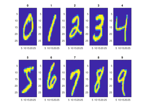
Figure 1: 10 random MNIST test images. Above each image is its label.

For the EMNIST dataset, we will focus on the EMNIST Digits subset containing images of handwritten digits with 4000 test images and 24000 training images for each digit $0,1,...,9$. When writing EMNIST below, we refer to this subset.

Contrary to MNIST, the images in EMNIST look more like various types of shapes than images of handwritten digits, see e.g. Figure 2.

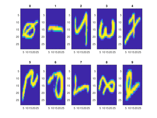
Figure 2: 10 random EMNIST test images. Above each image is its label.

Since we did not find any result regarding human error rate on EMNIST, we estimated our own error rate and it turned out to be more than 1.5%. We also tried shallow neural networks (with a few hidden layers) and noticed that the error rate was more than 1.3% for these networks. So this dataset is much more difficult for classification.

We will also use MNIST Balanced dataset that is constructed in the following way. Let us enumerate the images in the MNIST dataset for each digit in the order that they appear starting with the training set and then the test set. Then, for example, for digit 0 we will have in total 5923 training images enumerated 1 - 5923 and 980 test images enumerated 5924 - 6903. Note that there are different number of images in the training and test sets for different digits. To make this dataset more similar to EMNIST we will change the sets of training and test sets in the standard MNIST dataset. More precisely, the training set will consist of the first 6000 images for each digit and the test set will consist of all remaining images. This new dataset we will call MNIST Balanced dataset. Note that this dataset is uniform in size of training sets with respect to the different digits.

The recent survey [1] provides a detailed overview of image classification on MNIST and EMNIST, covering both traditional methods and ANNs, where further references can be found.

4 WNN algorithm

4.1 An algorithm.

As we wrote above all images in MNIST and EMNIST are greyscale images of size 28 $\times\$28, i.e. they consist of 784 pixels and on each pixel the image takes an integer value between 0 and 255. For each of the 784 pixels, we will consider a square ‘window’ $W$ centered at the pixel with side length S where S is an odd positive integer. Each window $W$ therefore consists of $S^{2}$ pixels. For simplicity of notation, we will from now on refer to S as the size of the window. Note that for some pixels, the window $W$ will extend beyond the image boundaries. We will set the values of the pixels in $W$ which falls outside the screen equal to zero.

Denote by $A_{train}^{i}$, $i=1,\dots,10$, the class of training images that corresponds to digit $i-1$. By $B_{test}^{i}$ , we denote the corresponding class of test images for digit $i-1$. Let $B$ be some test image. We will calculate distances between $B$ and $A_{train}^{i}$ on the window $W$ according to

$$dist_{W}(B,A_{train}^{i})=\min_{A\in A_{train}^{i}}(\sum_{y\in W}(B(y)-A(y))^{2})^{1/2},$$

so $dist_{W}(B,A_{train}^{i})$ is a discrete analog of local approximation in metric of $L^{2}$ if instead of polynomials $P$ of degree strictly less than $k$ we will consider the set $A_{train}^{i}$.

Next, for each class $A_{train}^{i}$ we take into account the distances on all windows and define

$$Dist(B,A_{train}^{i})=(\sum_{W}dist_{W}(B,A_{train}^{i})^{2})^{1/2}.$$

Note that this formula is a discrete analog of the formula (2.2).

Our algorithm classifies image $B$ as an image from the class $B_{test}^{i}$ if

$$Dist(B,A_{train}^{i})=\min_{j=1,...,10}Dist(B,A_{train}^{j})\text{.}$$

In the case when minimum is attained for several indices $1\leq i_{1}<...<i_{n}\leq 10$ we will (arbitrarily) classify $B$ as an image of the class $B_{test}^{i_{1}}$. It can be noted that such a situation has not occurred in our investigations.

4.2 Size of used windows

To apply the algorithm we need to know the size $S$ of used windows. To find it we did experiments with the MNIST Balanced dataset.

The next table (Table 1) shows how many classification errors WNN produces for different window sizes $S$ (indicated by WNN$S$, for example by WNN11 we will mean the case when $S=11$ ). By ’NN’ we denote the case when $S=55$, i.e. we actually have only one window and our classification algorithm coincides with the usual Nearest Neighbour algorithm. We see that WNN with $S=11$ is the best and has 106 errors from 10000 test images, i.e. the error rate is 1.06%. From this table we also see that the NN algorithm has 266 errors, i.e. a much higher error rate than the WNN11 algorithm.

Digit	NN	WNN3	WNN5	WNN7	WNN9	WNN11	WNN13	WNN15	WNN17	WNN19	WNN21	WNN23
0	7	17	7	4	4	5	5	5	5	5	5	5
1	10	123	35	14	6	5	5	7	6	7	7	7
2	37	28	13	8	8	7	9	10	12	14	14	16
3	48	42	16	16	16	14	12	13	18	19	19	21
4	28	14	7	6	5	6	8	8	8	9	12	14
5	2	5	1	1	2	2	2	2	2	2	2	2
6	12	28	21	11	10	8	7	7	7	7	8	8
7	43	76	38	28	19	18	16	20	22	25	26	27
8	41	20	9	7	11	12	13	15	13	13	15	15
9	38	54	38	31	29	29	30	27	28	29	31	33
Total	266	407	185	126	110	106	107	114	121	130	139	148

Table 1: Errors for different window sizes on MNIST Balanced.

5 Experiments on MNIST

It is expected that a larger training set will improve the performance of WNN. For this reason, we first extended the training set of MNIST Balanced (denoted ‘Set 0’) artificially by spatially shifting each image not more than one pixel in horizontal, vertical or in both directions at the same time. This gives eight new images for each original training image and in total $60000\cdot 9=540000$ training images. We refer to this set as ‘Set 1’. In a second step, each training image of Set 1 was rotated $\pm 5,\pm 25$ degrees generating an additional $2.16$ million training images. This set of $2.7$ million training images is denoted ‘Set 2’. Next, note that the digits are contained in the center $20\times 20$ pixels [10] of the image. For each image of Set 1 we then generated four new images by compressing/expanding the width or the height of this center part to $18$ and $22$ pixels. These compressed and expanded images together with Set 1 gives ‘Set 3’ with in total $2.7$ million images. Finally, the images of Sets 2 and 3 together constitute ‘Set 4’ which accordingly contains $4.86$ million unique images. In Table 2, we give the resulting number of errors of WNN11 for the different training sets.

Training set	Set 0	Set 1	Set 2	Set 3	Set 4
No. of training images	60000	540000	2700000	2700000	4860000
No. of test images	10000	10000	10000	10000	10000
No. of errors on test images	106	62	49	49	41
Error rate	1.06%	0.62%	0.49%	0.49%	0.41%

Table 2: Errors for WNN11 on MNIST Balanced when using different extensions of the training set.

We note that Set 4 gives the lowest error rate with 0.41%. Further expansions of the training set might give better results but we chose in this study to restrict ourselves to a few straightforward alternatives. When comparing with previously published work on NN-based methods, recall that the training and test sets considered in this study are not the standard ones of MNIST. However, when applying the WNN algorithm (with extension of the training set as above) on the MNIST standard set, we obtain an error rate of 0.48% which is lower than the best published result of 0.52% [8] that we are aware of.

6 Experiments on EMINST

Applying the WNN algorithm on EMNIST, window size 11 will be used based upon previous investigations on MNIST. The original training set of 240000 images is denoted by ‘Set 0’ and the extension of this set by spatially shifting not more than one pixel in horizontal, vertical or in both directions at the same time is referred to as ‘Set 1’. Adding rotations of $\pm 5,\pm 25$ degrees of each image to this set, a set denoted ‘Set 2’ is constructed. Finally, we consider an extension of Set 0 in terms of a spatial shift of maximum two pixels in horizontal, vertical or in both directions at the same time (denoted ‘Set 3’) and, as in the previous case, then extend Set 3 to include rotated images by $\pm 5,\pm 25$ degrees (denoted ‘Set 4’). These extensions are important. Indeed, the NN algorithm on EMNIST using the training images of Set 0 gives 625 errors (an error rate of 1.56%) and 385 errors (an error rate of 0.96%) using Set 4. The classification results of WNN using the different training sets are given in Table 3.

Training set	Set 0	Set 1	Set 2	Set 3	Set 4
No. of training images	240000	2160000	10800000	6000000	30000000
No. of test images	40000	40000	40000	40000	40000
No. of errors on test images	303	195	190	177	168
Error rate	0.76%	0.49%	0.48%	0.44%	0.42%

Table 3: Errors for WNN11 on EMNIST when using different extensions of the training set.

For comparison, we did experiments with one third of the training images (8000 images per digit) and did extension as for Set 4. The resulting number of errors for the WNN algorithm became 202 giving an error rate of 0.5%.

The best published result of a traditional classification method applied to EMNIST that we are aware of reports an error rate of 2.26% [6]. Therefore, even without extensions of the training set the result of WNN seems to be state of the art. Further, we obtain error rates which are much lower than the human error rate of 1.5%.

We would like to finish this section with a description of a more sophisticated version of the WNN algorithm. By using this version we can reduce the number of errors from 168 to 129 (an error rate of 0.32%) which is on par with the best neural network result (see [7]).

Let us briefly describe this algorithm. Let $A$ be a training image from Set 0. Denote by $A_{ext}$ the set which consists of $A$ and all its extensions as described above (so $A_{ext}$ consists of 125 images). Then we define the distance $d$ from the test image $B$ to $A$ as

$$d(B,A)=\Big{(}\sum_{W}(d_{W}(B,A_{ext}))^{2}\Big{)}^{1/2},$$ (6.1)

where $d_{W}(B,A_{ext})$ is the distance on window W from $B$ to $A_{ext}$ given by

$$d_{W}(B,A_{ext})=\min_{X\in A_{ext}}\Big{(}\sum_{w\in W}(B(w)-X(w))^{2}\Big{)}^{1/2}.$$ (6.2)

Next, the distance $D$ from $B$ to the training class $A^{i}_{train}$ from Set 0 (containing 24000 images for each digit $i-1$), $i=1,\dots,10$, is defined as

$$D(B,A_{train}^{i})=\min_{A\in A^{i}_{train}}d(B,A).$$ (6.3)

We classify $B$ as an image from the class $B_{test}^{i}$ if

$$D(B,A_{train}^{i})=\min_{j\in\left\{1,\dots,10\right\}}D(B,A_{train}^{j}).$$

This distance algorithm (denoted DWNN) gives 148 errors on EMNIST. Now for each test image $B$ we do predictions by WNN and DWNN. Usually these two predictions coincide, if they are different then we classify $B$ according to the NN classifier using the corresponding two training classes from Set 4 (containing $3\times 10^{6}$ images each). The resulting algorithm gives 129 errors on EMNIST.

7 An Algorithm for Decreasing the Number of Used Windows

It is of importance to decrease the computational cost of the WNN algorithm while maintaining its predictive performance. In this section we discuss one possible approach to this problem.

Denote by WNN${}_{W_{1},...,W_{K}}$ the WNN algorithm where the windows $W_{1},...,W_{K}$ are excluded, i.e. instead of $Dist(B,A_{train}^{i})$ we use

$$Dist_{W_{1},\dots,W_{K}}(B,A_{train}^{i})=\left(\sum dist_{W}(B,A_{train}^{i})^{2}\right)^{1/2},\,i=1,\dots,10$$

where we sum over all windows $W$ except $W_{1},...,W_{K}$.

We determine $W_{1},...,W_{K}$ in an iterative way according to the following. First, we calculate for each window $W$ the number of errors for the WNN_W algorithm. This number is denoted NE_W (number of errors when window $W$ is excluded). We then consider the set of windows $W$ with smallest number of errors NE_W. Usually this set contains many windows. For every window in the set, consider

$$GAP_{W}=\sum_{i=1}^{10}\sum_{B\in B_{test}^{i}}(Dist_{W}(B,A_{train}^{i})-\min_{j\in\left\{1,...,10\right\}}Dist_{W}(B,A_{train}^{j}))$$

and exclude the window $W$ for which GAP_W is maximal. To explain the idea behind this algorithm note that if the test image $B$ is in class $B_{test}^{i}$ and is predicted correctly by WNN then

$$Dist_{W}(B,A_{train}^{i})-\min_{j=1,...,10}Dist_{W}(B,A_{train}^{j})=0$$

and if $B$ is not predicted correctly then

$$Dist_{W}(B,A_{train}^{i})-\min_{j=1,...,10}Dist_{W}(B,A_{train}^{j})>0.$$

So if all test images are predicted correctly then $GAP_{W\text{ }}=0$ and the idea is to exclude the worst window.

Let us next consider an example on EMNIST. We apply the above algorithm to Set 4 (recall that it consists of 30$\times 10^{6}$ images). Then the number of errors with respect to the number of excluded windows $K$ can be seen in Figure 3.

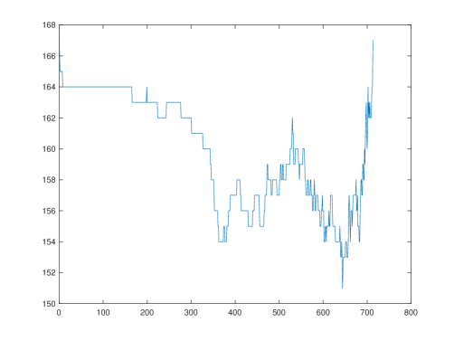
Figure 3: Number of errors versus number of excluded windows.

In particular when 100 windows are used, i.e. $K=684$, the number of errors will be 156. Using only 60 windows the number of errors increase to 167 which still is less than 168 which was obtained using all 784 windows.

However, note that constructing the set of excluded windows by using the whole test set is not correct. We therefore divide the test set of 40000 images randomly into two subsets: the validation set of 30000 images (3000 images for each digit) will be used for determining the number of excluded windows and the remaining set of 10000 images will be the new test set. The resulting graph of errors can be seen in Figure 4.

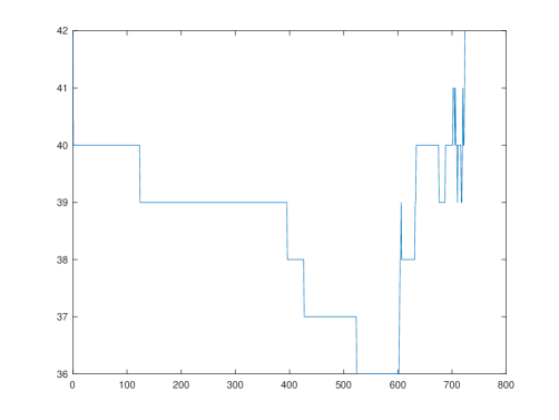
Figure 4: Number of errors versus number of excluded windows using validation set.

In particular, if we use just 50 windows then the number of errors will be 42 corresponding to an error rate of 0.42%. Recall that this error rate is the same as when using all 784 windows on the original test set.

References

- [1] A. Baldominos, Y. Saez, and P. Isasi. A survey of handwritten character recognition with MNIST and EMNIST. Appl. Sci., 9(15):3169, 2019.
- [2] C. M. Bishop. Pattern Recognition and Machine Learning. Springer-Verlag, New York, 2006.
- [3] Yu. Brudnyi. Spaces defined by means of local approximations. Trans. Moscow Math. Soc., 24:1422–1435, 1974.
- [4] G. Cohen, S. Afshar, J. Tapson, and A. van Schaik. EMNIST: an extension of MNIST to handwritten letters. arXiv:1702.05373, 2017.
- [5] E. Fix and J. L. Hodges Jr. Discriminatory analysis, non-parametric discrimination. USAF School of Aviation Medicine, Randolph Field, Tex. Project 21-49-004, Report no 4, Contract AF41(128)-31, 1951.
- [6] P. Ghadekar, S. Ingole, and D. Sonone. Handwritten digit and letter recognition using hybrid DWT-DCT with KNN and SVM classifier. In 2018 Fourth International Conference on Computing Communication Control and Automation (ICCUBEA), pages 1 – 6, 2018.
- [7] V. Jayasundara, S. Jayasekara, H. Jayasekara, J. Rajasegaran, S. Seneviratne, and R. Rodrigo. Textcaps : Handwritten character recognition with very small datasets. In 2019 IEEE Winter Conference on Applications of Computer Vision (WACV), pages 254–262, 2019.
- [8] D. Keysers, T. Deselaers, C. Gollan, and H. Ney. Deformation models for image recognition. IEEE Trans. Pattern Anal. Mach. Intell., 29(8):1422–1435, August 2007.
- [9] S. Kislyakov and N. Kruglyak. Extremal Problems in Interpolation Theory, Whitney-Besicovitch Coverings, and Singular Integrals. Birkhäuser, Basel, 2013.
- [10] Y. LeCun, C. Cortes, and C. J. C. Burges. The MNIST database of handwritten digits. http://yann.lecun.com/exdb/mnist/.
- [11] Y. LeCun, L. D. Jackel, L. Bottou, C. Cortes, J. S. Denker, H. Drucker, I. Guyon, U. A. Müller, E. Sackinger, P. Simard, and V. Vapnik. Learning algorithms for classification: A comparison on handwritten digit recognition. In J. H. Oh, C. Kwon, and S. Cho, editors, Neural Networks: The Statisical Mechanics Perspective, volume 1 of Progress in Neural Processing, pages 261–276. World Scientific, 1995.
- [12] J. Peetre. A theory of interpolation of normed spaces. Notas de Matemática, No. 39. Instituto de Matemática Pura e Aplicada, Conselho Nacional de Pesquisas, Rio de Janeiro, 1968.
- [13] E. Setterqvist, N. Kruglyak, and R. Forchheimer. An improved nearest neighbour classifier. arXiv:2204.13141, 2022.
- [14] B. W. Silverman and M. C. Jones. E. Fix and J. L. Hodges (1951): An important contribution to nonparametric discriminant analysis and density estimation. Commentary on Fix and Hodges (1951). Int. Statist. Rev., 57(3):233–238, 1989.