Temporal Forward-Backward Consistency, Not Residual Error, Measures the Prediction Accuracy of Extended Dynamic Mode Decomposition

Abstract

Extended Dynamic Mode Decomposition (EDMD) is a popular data-driven method to approximate the action of the Koopman operator on a linear function space spanned by a dictionary of functions. The accuracy of EDMD model critically depends on the quality of the particular dictionary span, specifically on how close it is to being invariant under the Koopman operator. Motivated by the observation that the residual error of EDMD, typically used for dictionary learning, does not encode the quality of the function space and is sensitive to the choice of basis, we introduce the novel concept of consistency index. We show that this measure, based on using EDMD forward and backward in time, enjoys a number of desirable qualities that make it suitable for data-driven modeling of dynamical systems: it measures the quality of the function space, it is invariant under the choice of basis, can be computed in closed form from the data, and provides a tight upper-bound for the relative root mean square error of all function predictions on the entire span of the dictionary.

I Introduction

Koopman operator theory has gained widespread attention in recent years for the study of dynamical systems, chiefly thanks to the linear structure of the operator despite nonlinearities in the system. In fact, the linearity of the Koopman operator leads to computationally efficient formulations to work with data. This provides a theoretically principled and explainable approach to the challenges posed by incorporating data-driven methods in the modeling, analysis, and control of dynamical systems. Given that the Koopman operator is generally infinite-dimensional, finding accurate finite-dimensional approximations for its action is of utmost importance. The first step to do so is to have a proper way to efficiently measure the quality of the subspace. This measure in turn can be used for subspace identification in optimization or neural network-based learning methods. Defining such a measure is, in turn, the goal of this paper.

Literature Review: The Koopman operator [1] provides an alternative representation of the evolution of dynamical systems in terms of observables rather than system trajectories. Despite possible nonlinearities in the system, the eigenfunctions of the Koopman operator evaluated on the system’s trajectories have linear temporal evolution, and this leads to efficient numerical methods used in complex system analysis [2, 3], estimation [4], control [5, 6, 7, 8], and robotics [9, 10], to name a few. Despite these appealing applications, the infinite-dimensional nature of the operator makes its direct use on digital computers challenging. Dynamic Mode Decomposition (DMD) [11] and its generalization Extended Dynamic Mode Decomposition (EDMD) [12] are popular data-driven methods to approximate the action of the Koopman operator on finite-dimensional spaces. EDMD in particular uses a dictionary of functions whose span specifies the finite-dimensional space of choice. The work in [13] studies the prediction accuracy of DMD while [14] provides several convergence results for EDMD as the number of data points and dimension of the dictionary go to infinity. The dependence of the EDMD’s prediction accuracy on the choice of the dictionary has led to a search for dictionaries whose span is close to being invariant under the Koopman operator [15]. The works in [16, 17] use methods based on neural networks for this task, while [18] directly learns the Koopman eigenfunctions spanning invariant subspaces. Moreover, the works in [19, 20] approximate finite-dimensional Koopman models relying on knowledge about the system’s attractors and their stability. In our previous work, we have provided efficient algebraic algorithms to identify exact Koopman-invariant subspaces [21, 22] or approximate them with tunable predefined accuracy [23].

Statement of Contributions: Our starting point is the observation that the residual error of EDMD, typically used for dictionary learning, does not necessarily measure the quality of the subspace spanned by the dictionary and, consequently, the prediction accuracy of EDMD on the subspace. To illustrate this point, we provide an example showing that one can choose a sequence of dictionaries spanning the same subspace that make the residual error arbitrarily close to zero. This motivates our goal of identifying better measures to assess the EDMD’s prediction accuracy and its dictionary’s quality. We define the notion of the consistency matrix and its spectral radius, which we term consistency index, which measures the deviation of the EDMD solutions forward and backward in time from being the inverse of each other. This is justified by the fact that if a subspace is Koopman invariant, the EDMD solutions applied forward and backward in time are the inverse of each other. We characterize various algebraic properties of the consistency index and show that it only depends on the data and the space spanned by the dictionary, and is hence invariant under changes of basis. We also establish that the square root of the consistency index provides a tight upper bound on the relative root mean square EDMD prediction error of all functions in the dictionary’s span.

II Preliminaries

We briefly recall basic facts about the Koopman operator [24] and Extended Dynamic Mode Decomposition [12].

Koopman Operator

Consider a dynamical system with state space $\mathcal{M}\subseteq\mathbb{R}^{n}$

$$x^{+}=T(x),\;x\in\mathcal{M}.$$ (1)

Let $\mathcal{F}$ be a vector space defined on $\mathbb{C}$ comprised of functions from $\mathcal{M}$ to $\mathbb{C}$ whose composition with $T$ also belong to $\mathcal{F}$. The Koopman operator associated with the dynamics is

$$\mathcal{K}f=f\circ T.$$ (2)

The operator is linear. Its eigenfunctions have linear evolution on the trajectories of the system, i.e., given eigenfunction $\phi$ with eigenvalue $\lambda$, $\phi(x^{+})=\phi\circ T(x)=\mathcal{K}\phi(x)=\lambda\phi(x)$. This results in a significant property of the Koopman eigendecomposition: given eigenpairs $\{(\lambda_{i},\phi_{i})\}_{i=1}^{N_{k}}$, the evolution of $f=\sum_{i=1}^{N_{k}}c_{i}\phi_{i}$ on a trajectory of the system starting from $x_{0}\in\mathcal{M}$ is $f(x(k))=\sum_{i=1}^{N_{k}}c_{i}\lambda_{i}^{k}\,\phi_{i}(x_{0})$, for $k\in\mathbb{N}$. This linear property is useful for both prediction and identification, as the linearity always holds even if the system is nonlinear. However, to completely capture the dynamics, one might need the space $\mathcal{F}$ to be infinite dimensional.

Extended Dynamic Mode Decomposition

The infinite-dimensional property of the Koopman operator prevents its direct use in practical data-driven settings. This leads naturally to constructing finite-dimensional approximations, e.g., using Extended Dynamic Mode Decomposition (EDMD). EDMD uses a dictionary $D:\mathcal{M}\to\mathbb{R}^{1\times N_{d}}$ containing $N_{d}$ functions, $D(x)=[d_{1}(x),\ldots,d_{N_{d}}(x)]$. To capture the dynamic behavior, EDMD uses data $X,Y\in\mathbb{R}^{N\times n}$ containing $N$ data snapshots gathered from system trajectories,

$$y_{i}=T(x_{i}),\,\forall i\in\{1,\dots,N\},$$ (3)

where $x_{i}^{T}$ and $y_{i}^{T}$ correspond to the $i$th rows of $X$ and $Y$. For convenience, we define the action of $D$ on a data matrix as $D(X)=[D(x_{1})^{T},D(x_{2})^{T},\ldots,D(x_{N})^{T}]^{T}$, where $x_{i}^{T}$ is the $i$th row of $X$. EDMD approximates the action of the Koopman operator on $\operatorname{span}(D)$ by solving

$$\underset{K}{\text{minimize}}\|D(Y)-D(X)K\|_{F}$$ (4)

which has the closed-form solution

$$K_{\operatorname{EDMD}}=\operatorname{EDMD}(D,X,Y):=D(X)^{\dagger}D(Y).$$ (5)

We rely on the following basic assumption.

Assumption II.1

(Full Rank Dictionary Matrices): $D(X)$ and $D(Y)$ have full column rank. $\square$

Assumption II.1 implies that the functions in $D$ are linearly independent, i.e., they form a basis for $\operatorname{span}(D)$ and the data are diverse enough to distinguish between the elements of $D$. Assumption II.1 ensures that $K_{\operatorname{EDMD}}$ is the unique solution for (4). One can use $K_{\operatorname{EDMD}}$ to approximate the Koopman eigenfunctions and, more importantly, the action of the operator on $\operatorname{span}(D)$. Given $f\in\operatorname{span}(D)$ in the form of $f(\cdot)=D(\cdot)v_{f}$ for $v_{f}\in\mathbb{C}^{N_{d}}$, one defines the EDMD predictor function for $\mathcal{K}f$ as

$$\mathfrak{P}_{\mathcal{K}f}(\cdot)=D(\cdot)K_{\operatorname{EDMD}}v_{f}.$$ (6)

The predictor’s quality depends on the quality of the dictionary. If $\operatorname{span}(D)$ is Koopman-invariant (i.e., $\mathcal{K}g\in\operatorname{span}(D)$ for all $g\in\operatorname{span}(D)$), the predictor (6) is exact (otherwise, the prediction is inexact for some functions in the space).

III Motivation and Problem Statement

The quality of the dictionary used for EDMD directly impacts its accuracy. Since in general the dynamics is unknown, it is important to use data to learn a proper dictionary tailored to the dynamics. The residual error of EDMD, $\|D(Y)-D(X)K_{\operatorname{EDMD}}\|_{F}$, is commonly used for this purpose as an objective function in optimization and neural network-based learning schemes. However, it is important to note that even though a high quality subspace (close to Koopman-invariant) leads to small residual error, the converse is not true: a dictionary $D$ with small residual error does not necessarily mean that EDMD’s prediction is accurate on $\operatorname{span}(D)$.

Example III.1

(Residual Error is not Invariant under Linear Transformation of Dictionary): Consider the linear system $x^{+}=0.5x$ and the vector space of functions $\mathcal{S}=\operatorname{span}\{x,x^{3}-x^{2}\}$. To apply EDMD, we gather $N=1000$ data snapshots from trajectories of the system with length of two time steps and initial conditions uniformly selected from $[-2,2]$, and form data matrices $X,Y\in\mathbb{R}^{N\times 1}$. We consider a family of dictionaries parameterized by $\alpha\in\mathbb{R}\setminus\{0\}$,

$$D_{\alpha}(x)=[x,x+\alpha(x^{3}-x^{2})].$$ (7)

Note that each $D_{\alpha}$ is a basis for $\mathcal{S}$, and all the dictionaries are related by nonsingular linear transformations. We also define two notions of prediction accuracy: the residual error $E$ of EDMD and its normalized version $E_{\operatorname{rel}}$,

$$E(\alpha)=\|D_{\alpha}(Y)-D_{\alpha}(X)K_{\alpha}\|_{F}, E_{\operatorname{rel}}(\alpha)=\frac{E(\alpha)}{\|D_{\alpha}(Y)\|_{F}},$$

where $K_{\alpha}=\operatorname{EDMD}(D_{\alpha},X,Y)$.

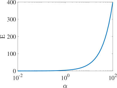
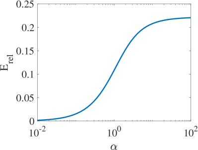
Figure 1: EDMD’s residual error (left) and relative residual error (right) as a function of $\alpha$ in (7).

Figure 1 shows the aforementioned notions of error versus the value of $\alpha\in[0.01,100]$. Figure 1 clearly demonstrates the sensitivity of errors to the choice of basis for $\mathcal{S}$ despite the invariance of $\operatorname{spec}(K_{\operatorname{EDMD},\alpha})$ under the choice of basis (see e.g., [23, Lemma 7.1]). By tuning $\alpha$, one can make both errors arbitrarily close to zero. As a result, using the residual error as a measure to assess the quality of the space or as an objective function in optimization or neural network-based dictionary learning schemes can lead to erroneous results. $\square$

Remark III.2

(Prediction Accuracy of Dictionary Elements versus Dictionary’s Span): Some applications only require short-term prediction of finitely many observables. In such cases, the residual error of EDMD may be useful: the observables of choice are fixed as elements of the dictionary and the rest of the functions composing the dictionary are learned by minimizing the residual error (which measures the average one time-step prediction error). However, such methods do not necessarily lead to a dictionary which spans an approximate Koopman-invariant subspace. $\square$

The observations in Example III.1 prompts us to search for a better measure of the dictionary’s quality and therefore the EDMD’s prediction accuracy. We formalize this next.

Problem III.3

(Characterization of EDMD’s Prediction Accuracy and the Dictionary’s Quality): Given a dictionary $D$ and data matrices $X$ and $Y$, under Assumption II.1, we aim to provide a data-driven measure of EDMD’s accuracy and the dictionary’s quality that

1. only depends on $\operatorname{span}(D)$, $X$, and $Y$, and hence is invariant under the choice of basis for $\operatorname{span}(D)$, i.e., given $D^{\prime}$ as an alternative basis for $\operatorname{span}(D)$, the accuracy measures calculated based on $D$ and $D^{\prime}$ are equal;

2. provides a data-driven bound on the distance between $\mathcal{K}f$ and its EDMD prediction $\mathfrak{P}_{\mathcal{K}f}$ for all functions $f\in\operatorname{span}(D)$;

3. can be computed using a closed-form formula (for implementation in optimization solvers). $\square$

IV Temporal Forward-Backward Consistency

Here, we take the first step towards finding an appropriate measure for EDMD’s prediction accuracy by comparing the solutions of EDMD forward and backward in time. Throughout the paper, we use the following notation for forward and backward EDMD matrices

$$K_{F}=\operatorname{EDMD}(D,X,Y)=D(X)^{\dagger}D(Y),$$ (8a)

$$K_{B}=\operatorname{EDMD}(D,Y,X)=D(Y)^{\dagger}D(X).$$ (8b)

We rely on the observation that if the dictionary spans a Koopman-invariant subspace, then $K_{F}K_{B}=I$. Otherwise, the forward and backward EDMD matrices will not be the inverse of each other, which motivates the next definition.

Definition IV.1

(Consistency Matrix and Index): Given dictionary $D$ and data matrices $X$ and $Y$, the consistency matrix is $M_{C}(D,X,Y)=I-K_{F}K_{B}$ and the consistency index is $\mathcal{I}_{C}(D,X,Y)=\operatorname{sprad}\big{(}M_{C}(D,X,Y)\big{)}$. $\square$

For convenience, we refer to $M_{C}(D,X,Y)$ and $\mathcal{I}_{C}(D,X,Y)$ as $M_{C}$ and $\mathcal{I}_{C}$ when the context is clear. Next, we show that the eigenvalues of the consistency matrix are invariant under linear transformations of the dictionary.

Proposition IV.2

(Consistency Matrix’s Spectrum is Invariant under Linear Transformation of Dictionary): Let $D$ and $\tilde{D}$ be two dictionaries such that $\tilde{D}(\cdot)=D(\cdot)R$, where $R$ is an invertible matrix. Moreover, given data matrices $X$ and $Y$ let Assumption II.1 hold. Then,

1. $M_{C}(\tilde{D},X,Y)=R^{-1}M_{C}(D,X,Y)R$;

2. $\operatorname{spec}\big{(}M_{C}(D,X,Y)\big{)}=\operatorname{spec}\big{(}M_{C}(\tilde{D},X,Y)\big{)}$.

Proof:

Note that part (b) directly follows from part (a) and the fact that similarity transformations preserve the eigenvalues. To show part (a), define for convenience,

$$K_{F}=D(X)^{\dagger}D(Y), K_{B}=D(Y)^{\dagger}D(X),$$

$$\tilde{K}_{F}=\tilde{D}(X)^{\dagger}\tilde{D}(Y), \tilde{K}_{B}=\tilde{D}(Y)^{\dagger}\tilde{D}(X).$$

We start by showing that $K_{F}K_{B}$ and $\tilde{K}_{F}\tilde{K}_{B}$ are similar. By definition, one can write

$$\tilde{K}_{F}\tilde{K}_{B}=\tilde{D}(X)^{\dagger}\tilde{D}(Y)\tilde{D}(Y)^{\dagger}\tilde{D}(X).$$ (9)

Moreover, given Assumption II.1 and the definition of $\tilde{D}$,

$$\tilde{D}(X)^{\dagger}=\big{(}\tilde{D}(X)^{T}\tilde{D}(X)\big{)}^{-1}\tilde{D}(X)^{T}$$

$$=\big{(}R^{T}D(X)^{T}D(X)R\big{)}^{-1}R^{T}D(X)^{T}=R^{-1}D(X)^{\dagger}.$$ (10)

Equations (9)-(IV), in conjunction with the fact that $\tilde{D}(Y)\tilde{D}(Y)^{\dagger}=D(Y)D(Y)^{\dagger}$ (cf. Lemma A.1 in the appendix), imply $\tilde{K}_{F}\tilde{K}_{B}=R^{-1}K_{F}K_{B}R$ directly leading to the required identity following Definition IV.1. ∎

According to Proposition IV.2, the spectrum of the consistency matrix is a property of the data and the vector space spanned by the dictionary, as opposed to the dictionary itself. This property is consistent with the requirement in Problem III.3(a). Next, we further investigate the eigendecomposition of the consistency matrix.

Lemma IV.3

(Consistency Matrix’s Properties): Given Assumption II.1, the consistency matrix $M_{C}(D,X,Y)$ satisfies:

1. it is similar to a symmetric matrix;

2. it is diagonalizable with a complete set of eigenvectors;

3. $\operatorname{spec}\big{(}M_{C}(D,X,Y)\big{)}\subset[0,1]$.

Proof:

(a) Given Assumption II.1, there exists an invertible matrix $R$ such that the columns of $D(X)R$ are orthonormal. Define the dictionary $\tilde{D}(\cdot)=D(\cdot)R$. Note that $\tilde{D}(X)^{T}\tilde{D}(X)=I_{N_{d}}$ and hence $\tilde{D}(X)^{\dagger}=\big{(}\tilde{D}(X)^{T}\tilde{D}(X)\big{)}^{-1}\tilde{D}(X)^{T}=\tilde{D}(X)^{T}$. Hence,

$$M_{C}(\tilde{D},X,Y)=I-\tilde{D}(X)^{T}\tilde{D}(Y)\tilde{D}(Y)^{\dagger}\tilde{D}(X).$$

Noting that $\tilde{D}(Y)\tilde{D}(Y)^{\dagger}$ is symmetric, we deduce that $M_{C}(\tilde{D},X,Y)$ is symmetric. Then (a) directly follows by the definition of $R$ and Proposition IV.2(a).

(b) The proof directly follows from part (a) and the fact that symmetric matrices are diagonalizable and have a complete set of eigenvectors.

(c) From part (a), we deduce that $M_{C}(D,X,Y)$ has real eigenvalues. Since $M_{C}(D,X,Y)=I-D(X)^{\dagger}D(Y)D(Y)^{\dagger}D(X)$, we only need to show

$$\operatorname{spec}\big{(}D(X)^{\dagger}D(Y)D(Y)^{\dagger}D(X)\big{)}\subset[0,1].$$ (11)

Consider an eigenvector $v\in\mathbb{R}^{N_{d}}\setminus\{0\}$ with eigenvalue $\mu$, i.e., $D(X)^{\dagger}D(Y)D(Y)^{\dagger}D(X)v=\mu v$. Multiplying both sides from the left by $D(X)$ and defining $w=D(X)v$ leads to $D(X)D(X)^{\dagger}D(Y)D(Y)^{\dagger}w=\mu w$. Next, multiplying this equation from the left by $w^{T}$,

$$w^{T}D(X)D(X)^{\dagger}D(Y)D(Y)^{\dagger}w=\mu\|w\|_{2}^{2}.$$ (12)

The fact that $D(X)D(X)^{\dagger}$ is symmetric and represents the orthogonal projection operator on $\mathcal{R}(D(X))$, in conjunction with $w\in\mathcal{R}(D(X))$, allows us to write $w^{T}D(X)D(X)^{\dagger}=w^{T}$. This, combined with (12), yields $\mu=\frac{w^{T}D(Y)D(Y)^{\dagger}w}{\|w\|_{2}^{2}}$. Hence, $\lambda_{\min}(D(Y)D(Y)^{\dagger})\leq\mu\leq\lambda_{\max}(D(Y)D(Y)^{\dagger})$. However, since $D(Y)D(Y)^{\dagger}$ is an orthogonal projection operator, we have $\operatorname{spec}(D(Y)D(Y)^{\dagger})\subset[0,1]$. Hence, $\mu\in[0,1]$, leading to (11), concluding the proof. ∎

From Lemma IV.3, the consistency matrix is similar to a positive semidefinite matrix. The larger the eigenvalues of $M_{C}$, the more inconsistent the forward and backward EDMD models get. Also, from Lemma IV.3, $\mathcal{I}_{C}=\lambda_{\max}(M_{C})\in[0,1]$. Intuitively, the consistency index determines the quality of the subspace spanned by the dictionary and the prediction accuracy of EDMD on it. This is formalized next.

V Consistency Index Determines EDMD’s Prediction Accuracy on Data

Our main result states that the square root of the consistency index is a tight upper bound for the relative root mean square prediction error of EDMD.

Theorem V.1

($\sqrt{\mathcal{I}_{C}}$ Bounds the Relative Root Mean Square Error (RRMSE) of EDMD): For dictionary $D$ and data matrices $X,Y$, under Assumption II.1,

$$\operatorname{RRMSE_{\max}} :=\max_{f\in\operatorname{span}(D)}\frac{\sqrt{\frac{1}{N}\sum_{i=1}^{N}|\mathcal{K}f(x_{i})-\mathfrak{P}_{\mathcal{K}f}(x_{i})|^{2}}}{\sqrt{\frac{1}{N}\sum_{i=1}^{N}|\mathcal{K}f(x_{i})|^{2}}}$$

$$=\sqrt{\mathcal{I}_{C}(D,X,Y)}.$$

where $x_{i}$ is the $i$th row of $X$ and $\mathfrak{P}_{\mathcal{K}f}$ is defined in (6).

Note that the combination of Definition IV.1, Lemma IV.3, and Theorem V.1 mean that $\sqrt{\mathcal{I}_{C}(D,X,Y)}$ satisfies all the requirements in Problem III.3. Before proving the result, we first remark its importance regarding function predictions.

Remark V.2

($\sqrt{\mathcal{I}_{C}}$ Determines the Relative $L_{2}$-norm Error of EDMD’s Prediction under Empirical Measure): Given that the elements of $\operatorname{span}(D)$ and their composition with $T$ are measurable and considering the empirical measure $\mu_{X}=\frac{1}{N}\sum_{i=1}^{N}\delta_{x_{i}}$, where $\delta_{x_{i}}$ is the Dirac measure defined based on the $i$th row of $X$, one can rewrite $\operatorname{RRMSE_{\max}}$ as

$$\operatorname{RRMSE_{\max}}\!=\max_{f\in\operatorname{span}(D)}\frac{\|\mathcal{K}f-\mathfrak{P}_{\mathcal{K}f}\|_{L_{2}(\mu_{X})}}{{\|\mathcal{K}f\|_{L_{2}(\mu_{X})}}}=\sqrt{\mathcal{I}_{C}}. \square$$

To prove Theorem V.1, we first provide the following alternative expression of the consistency index.

Theorem V.3

(Consistency Index and Difference of Projections): Given Assumption II.1,

$$\sqrt{\mathcal{I}_{C}(D,X,Y)}=\operatorname{sprad}\big{(}D(Y)D(Y)^{\dagger}-D(X)D(X)^{\dagger}\big{)}.$$

Proof:

From Lemma IV.3, we have $\mathcal{I}_{C}=\lambda_{\max}(M_{C})$. We use the following notation throughout the proof,

$$\lambda_{\max}=\mathcal{I}_{C},\,\mathcal{P}_{D(X)}=D(X)D(X)^{\dagger},\,\mathcal{P}_{D(Y)}=D(Y)D(Y)^{\dagger}.$$

Note that $\mathcal{P}_{D(X)}$ and $\mathcal{P}_{D(Y)}$ are projection operators on $\mathcal{R}(D(X))$ and $\mathcal{R}(D(Y))$, resp. By Definition IV.1, given an eigenvalue $\lambda\in[0,1]$ of $M_{C}$ with eigenvector $v\neq 0$,

$$M_{C}v=\lambda v\Leftrightarrow K_{F}K_{B}v=(1-\lambda)v.$$ (13)

We consider the cases (i) $\lambda_{\max}=0$, (ii) $\lambda_{\max}=1$, and (iii) $\lambda_{\max}\in(0,1)$ separately.

Case (i): $\lambda_{\max}=0$. In this case, from Lemma IV.3, we deduce $M_{C}=0$. Consequently, $K_{F}K_{B}=I$. By multiplying both sides from the left by $D(X)$ and collecting the terms, we have $\mathcal{P}_{D(X)}\mathcal{P}_{D(Y)}D(X)=D(X)$. Hence, one can write

$$\mathcal{P}_{D(X)}\mathcal{P}_{D(Y)}z=z,\;\forall z\in\mathcal{R}(D(X)).$$ (14)

Based on [27, summary table in p. 298], we deduce

$$\mathcal{P}_{D(X)}\mathcal{P}_{D(Y)}w=w\Leftrightarrow w\in\mathcal{R}(D(X))\cap\mathcal{R}(D(Y)).$$ (15)

Using (14)-(15), one can write $\mathcal{R}(D(X))\subseteq\mathcal{R}(D(X))\cap\mathcal{R}(D(Y))$ and consequently $\mathcal{R}(D(X))\subseteq\mathcal{R}(D(Y))$. By a similar argument as above and swapping $K_{F}$ with $K_{B}$ and $D(X)$ with $D(Y)$, one can also deduce $\mathcal{R}(D(Y))\subseteq\mathcal{R}(D(X))$. Hence, $\mathcal{R}(D(X))=\mathcal{R}(D(Y))$. Moreover, since the orthogonal projection on a subspace is unique, we have $\mathcal{P}_{D(Y)}-\mathcal{P}_{D(X)}=0$, concluding the proof for this part.

Case (ii): $\lambda_{\max}=1$. By setting $\lambda=\lambda_{\max}$ in (13), multiplying both sides from the left by $D(X)$, defining $w:=D(X)v$, we have

$$\mathcal{P}_{D(X)}\mathcal{P}_{D(Y)}w=0.$$ (16)

Hence, noting that $w\neq 0$ (based on Assumption II.1 and the fact that $v\neq 0$), we can deduce it is an eigenvector of $\mathcal{P}_{D(X)}\mathcal{P}_{D(Y)}$ with eigenvalue $0$. We show next that $w\in\mathcal{R}(D(X))\cap\mathcal{R}(D(Y))^{\perp}$. One can write $\mathcal{R}(D(X))$ as the direct sum of the orthogonal subspaces $\mathcal{R}(D(X))\cap\mathcal{R}(D(Y))$ and $\mathcal{R}(D(X))\cap\mathcal{R}(D(Y))^{\perp}$. Hence, we uniquely decompose $w\in\mathcal{R}(D(X))$ as $w=w_{D(Y)}+w_{D(Y)^{\perp}}$, where $w_{D(Y)}\in\mathcal{R}(D(X))\cap\mathcal{R}(D(Y))$ and $w_{D(Y)^{\perp}}\in\mathcal{R}(D(X))\cap\mathcal{R}(D(Y))^{\perp}$. Noting that $\mathcal{P}_{D(Y)}w_{D(Y)^{\perp}}=0$ and $\mathcal{P}_{D(Y)}w_{D(Y)}=w_{D(Y)}$, we get from (16) that $\mathcal{P}_{D(X)}\mathcal{P}_{D(Y)}w=\mathcal{P}_{D(X)}w_{D(Y)}=0$. Since $w_{D(Y)}\in\mathcal{R}(D(X))$, we deduce $w_{D(Y)}=0$ and consequently,

$$w=w_{D(Y)^{\perp}}\in\mathcal{R}(D(X))\cap\mathcal{R}(D(Y))^{\perp}.$$

Therefore, $(\mathcal{P}_{D(Y)}-\mathcal{P}_{D(X)})w=-w$ and, given that $w\neq 0$, we deduce that $\mathcal{P}_{D(Y)}-\mathcal{P}_{D(X)}$ has an eigenvalue equal to $-1$. Since $\operatorname{spec}(\mathcal{P}_{D(Y)}-\mathcal{P}_{D(X)})\subset[-1,1]$, cf. [27, Lemma 1], we conclude $\operatorname{sprad}(\mathcal{P}_{D(Y)}-\mathcal{P}_{D(X)})=1$. The proof concludes by noting that $\mathcal{I}_{C}=\lambda_{\max}=1$.

Case (iii): $\lambda_{\max}\in(0,1)$. Using Lemma A.2 and the closed-form expressions of $K_{F}$, $K_{B}$, $\mathcal{P}_{D(X)}$, and $\mathcal{P}_{D(Y)}$,

$$\operatorname{spec}_{\neq 0}(K_{F}K_{B})=\operatorname{spec}_{\neq 0}(\mathcal{P}_{D(X)}\mathcal{P}_{D(Y)}).$$ (17)

Given $\mu\in(0,1)$, from [27, Theorems 1-2], $\mu\in\operatorname{spec}_{\neq 0}(\mathcal{P}_{D(X)}\mathcal{P}_{D(Y)})$ if and only if $\{\pm\sqrt{1-\mu}\}\subset\operatorname{spec}_{\neq 0}\big{(}\mathcal{P}_{D(Y)}-\mathcal{P}_{D(X)}\big{)}$. Setting $\mu=1-\lambda$, $\lambda\in(0,1)$, one can use this in conjunction with (13) and (17) to write

$$\lambda\in\operatorname{spec}_{\neq 0}(M_{C})\Leftrightarrow\{\pm\sqrt{\lambda}\}\subset\operatorname{spec}_{\neq 0}\big{(}\mathcal{P}_{D(Y)}-\mathcal{P}_{D(X)}\big{)}.$$

This, in conjunction with [27, Theorem 1] and the fact that $\operatorname{sprad}\big{(}\mathcal{P}_{D(Y)}-\mathcal{P}_{D(X)}\big{)}\leq 1$ (cf. [27, Lemma 1]), shows that if $\operatorname{sprad}\big{(}\mathcal{P}_{D(Y)}-\mathcal{P}_{D(X)}\big{)}<1$, then the result holds. To conclude the proof, we need to show that $\operatorname{sprad}\big{(}\mathcal{P}_{D(Y)}-\mathcal{P}_{D(X)}\big{)}=1$ is not true. By contradiction, suppose this is the case, then at least one of the following holds:

1. $\exists w_{1}\in\mathbb{R}^{N}\setminus\{0\};\;\big{(}\mathcal{P}_{D(Y)}-\mathcal{P}_{D(X)}\big{)}w_{1}=-w_{1}$,

2. $\exists w_{2}\in\mathbb{R}^{N}\setminus\{0\};\;\big{(}\mathcal{P}_{D(Y)}-\mathcal{P}_{D(X)}\big{)}w_{2}=w_{2}$.

For case (a), based on [27, summary table in p. 298],

$$w_{1}\in\mathcal{R}(D(X))\cap\mathcal{R}(D(Y))^{\perp}.$$

Now, consider the vector $p_{1}\neq 0$ with $w_{1}=D(X)p_{1}$. Consequently, one can write $K_{F}K_{B}p_{1}=D(X)^{\dagger}\mathcal{P}_{D(Y)}w_{1}=0$, where in the last equality we have used $w_{1}\perp\mathcal{R}(D(Y))$. However, this implies that $M_{C}p_{1}=p_{1}$, contradicting the fact that $\lambda_{\max}\in(0,1)$.

For case (b), note that $w_{2}\in\mathcal{R}(D(Y))\cap\mathcal{R}(D(X))^{\perp}$ (see e.g., [27, summary table in p. 298]). Consider the vector space $\mathcal{S}=\mathcal{R}(D(Y))\cap\mathcal{R}(w_{2})^{\perp}$. Clearly $\dim\mathcal{S}<\dim\mathcal{R}(D(Y))=\dim\mathcal{R}(D(X))$. Consequently, there exists a non-zero vector $w^{*}\in\mathcal{R}(D(X))$ such that $w^{*}\perp\mathcal{S}$. Also, $w^{*}\perp\mathcal{R}(w_{2})$ since $w_{2}\perp\mathcal{R}(D(X))$. Hence, by noting that $\mathcal{R}(D(Y))$ is the direct sum of $\mathcal{S}$ and $\mathcal{R}(w_{2})$, one can conclude $w^{*}\in\mathcal{R}(D(X))\cap\mathcal{R}(D(Y))^{\perp}$ and, as a result, we have $\big{(}\mathcal{P}_{D(Y)}-\mathcal{P}_{D(X)}\big{)}w^{*}=-w^{*}$. Since $w^{*}$ satisfies the identity in case (a), the proof follows by replacing $w_{1}$ with $w^{*}$ in the proof of case (a). ∎

Remark V.4

(Geometric Connections to Grassmannians): Theorem V.3 establishes a link between the consistency index and the spectral radius of the difference of projection matrices. Given proper confinement of subspaces with fixed dimension to a Grassmannian, see e.g. [28], the consistency index can be viewed as a metric measuring the distance (by encoding angles) between vector spaces of fixed dimension. Similar ideas based on the difference of projections have been used in the context of dynamic mode decomposition [29]. Even if the dimension of the vector spaces is not fixed, the consistency index and difference of projections still can be used through results similar to Theorem V.1. This is especially relevant if the dimension of the Koopman-invariant subspace is unknown, see e.g. [23]. $\square$

We are finally ready to prove Theorem V.1.

Proof:

(Theorem V.1): We use the following notation throughout the proof: $\mathcal{P}_{D(X)}=D(X)D(X)^{\dagger}$, $\mathcal{P}_{D(Y)}=D(Y)D(Y)^{\dagger}$, and $s=\operatorname{sprad}(\mathcal{P}_{D(Y)}-\mathcal{P}_{D(X)})$. Note that, from Theorem V.3, $s=\sqrt{\mathcal{I}_{C}(D,X,Y)}$. Given an arbitrary function $f(\cdot)=D(\cdot)v_{f}\in\operatorname{span}(D)$, with $v_{f}\in\mathbb{C}^{N_{d}}$, one can use (2), the predictor (6) with $K_{F}=K_{\operatorname{EDMD}}=\operatorname{EDMD}(D,X,Y)$, and the relationship between the rows of $X$ and $Y$ in (3) to write

$$\operatorname{RRMSE}_{f} :=\frac{\sqrt{\sum_{i=1}^{N}|D(y_{i})v_{f}-D(x_{i})K_{F}v_{f}|^{2}}}{\sqrt{\sum_{i=1}^{N}|D(y_{i})v_{f}|^{2}}}$$

$$=\frac{\|D(Y)v_{f}-D(X)K_{F}v_{f}\|_{2}}{\|D(Y)v_{f}\|_{2}}$$ (18)

Noting that $D(Y)=\mathcal{P}_{D(Y)}D(Y)$, one can write

$$\|D(Y)v_{f}-D(X)K_{F}v_{f}\|_{2} =\|(\mathcal{P}_{D(Y)}-\mathcal{P}_{D(X)})D(Y)v_{f}\|_{2}$$

$$\leq s\|D(Y)v_{f}\|_{2},$$ (19)

where the last inequality holds since the matrix $\mathcal{P}_{D(Y)}-\mathcal{P}_{D(X)}$ is symmetric and therefore its spectral radius is equal to its induced 2-norm. Based on (V)-(V), we have $\operatorname{RRMSE}_{f}\leq s$. Hence, by definition of $\operatorname{RRMSE_{\max}}$ in the statement of the result, we have

$$\operatorname{RRMSE_{\max}}=\max_{f\in\operatorname{span}(D)}\operatorname{RRMSE}_{f}\leq s$$ (20)

Now, we prove that the equality in (20) holds. We consider three cases: (i) $s=0$ (ii) $s=1$ or (iii) $s\in(0,1)$.

Case (i): Since $\operatorname{RRMSE_{\max}}\geq 0$ by definition, in this case $\operatorname{RRMSE_{\max}}=0$ follows directly.

Case (ii): In this case, there exists a nonzero vector $p^{*}\in\mathcal{R}(D(Y))\cap\mathcal{R}(D(X))^{\perp}$. Let $v^{*}$ be such that $p^{*}=D(Y)v^{*}$. Using (V) for $v^{*}$ instead of $v_{f}$, and the properties of $p^{*}$, one can write $\|D(Y)v^{*}-D(X)K_{F}v^{*}\|_{2}=\|\mathcal{P}_{D(Y)}D(Y)v^{*}\|_{2}=\|D(Y)v^{*}\|_{2}$. Hence, for the function $f^{*}(\cdot)=D(\cdot)v^{*}\in\operatorname{span}(D)$, one can use (V) to see that $\operatorname{RRMSE}_{f^{*}}=1=s$. Hence, equality holds in (20).

Case (iii): In this case $s\in(0,1)$ and based on [27, Theorem 1], the matrix $\mathcal{P}_{D(Y)}-\mathcal{P}_{D(X)}$ has two eigenvalues $\pm s$ with corresponding orthogonal eigenvectors $v_{+s},v_{-s}\in\mathbb{R}^{N_{d}}$. Moreover, based on [27, Theorem 1(a)], $\mathcal{P}_{D(Y)}v_{+s}\in\operatorname{span}(v_{+s},v_{-s})$. Hence, for some $\alpha,\beta\in\mathbb{R}$, we have

$$q^{*}:=\mathcal{P}_{D(Y)}v_{+s}=\alpha v_{+s}+\beta v_{-s}.$$

Let $r^{*}$ be such that $q^{*}=D(Y)r^{*}$. Now, based on the first part of (V) for $r^{*}$ instead of $v_{f}$, we have

$$\|D(Y)r^{*}-D(X)K_{F}r^{*}\|_{2}=\|(\mathcal{P}_{D(Y)}-\mathcal{P}_{D(X)})D(Y)r^{*}\|_{2}$$

$$=\|(\mathcal{P}_{D(Y)}-\mathcal{P}_{D(X)})(\alpha v_{+s}+\beta v_{-s})\|_{2}=s\|\alpha v_{+s}-\beta v_{-s}\|_{2}$$

$$=s\|\alpha v_{+s}+\beta v_{-s}\|_{2}=s\|D(Y)r^{*}\|_{2},$$ (21)

where in the third and fourth equalities we have used the definition of $v_{+s}$ and $v_{-s}$ and their orthogonality. Now, for the function $g^{*}(\cdot)=D(\cdot)r^{*}\in\operatorname{span}(D)$, one can use (V) to see that $\operatorname{RRMSE}_{g^{*}}=s$. Hence, the equality in (20) holds, and this concludes the proof. ∎

Remark V.5

(Working with Consistency Matrix is More Efficient than the Difference of Projections): According to Theorems V.1 and V.3, one can use the consistency matrix $M_{C}\in\mathbb{R}^{N_{d}\times N_{d}}$ or the difference of projections $D(Y)D(Y)^{\dagger}-D(X)D(X)^{\dagger}\in\mathbb{R}^{N\times N}$ interchangeably to compute the relative root mean square error. However, note that the size of the consistency matrix depends on the dictionary $N_{d}$, while the size of the difference of projections depends on the size of data $N$. In most practical settings $N\gg N_{d}$, and consequently, working with the consistency matrix is more efficient. In fact, given moderate to large data sets, even saving the difference of projections matrix in the memory may be infeasible. The calculation of the consistency matrix requires solving two least-squares problems, which can be done recursively for large data sets. $\square$

Remark V.6

(Efficient Computation of the Consistency Index): The consistency index is defined as the spectral radius of the consistency matrix and can be computed as such. One can also use the following to compute it more efficiently: (i) the consistency index is the maximum eigenvalue of a matrix with nonnegative real eigenvalues (cf. Lemma IV.3(c)); (ii) given an appropriate change of coordinates making $D(X)^{T}D(X)=I$ (see proof of Lemma IV.3(a)), the consistency matrix becomes positive semi-definite. Hence, in optimization-based dictionary learning, one can add a constraint $D(X)^{T}D(X)=I$ and minimize the 2-norm of the consistency matrix (which equals the maximum eigenvalue for positive semi-definite matrices). $\square$

VI Conclusions

We have introduced the concept of consistency index, a data-driven measure that quantifies the accuracy of the EDMD method on a finite-dimensional functional space generated by a dictionary of functions. The consistency index is invariant under the choice of basis of the functional space, is computable in closed form, and corresponds to the relative root mean squared error. Future work will build on the measure introduced here to design algebraic algorithms that find dictionaries with EDMD predictions of a predetermined level of accuracy and use the consistency index as an objective for optimization and neural network-based methods to identify dictionaries including the system state that span spaces that are close to being Koopman-invariant.

Appendix A Basic Algebraic Results

Here, we recall two results that are used in the proofs.

Lemma A.1

Let $B_{1},B_{2}\in\mathbb{R}^{m\times n}$ be matrices such that $\mathcal{R}(B_{1})=\mathcal{R}(B_{2})$. Then $B_{1}B_{1}^{\dagger}=B_{2}B_{2}^{\dagger}$. $\square$

The proof follows from the uniqueness of the orthogonal projection operator on a subspace.

Lemma A.2

([30, Proposition 4.4.10]): Let $A\in\mathbb{R}^{m\times n}$ and $B\in\mathbb{R}^{n\times m}$. Then, $\operatorname{spec}_{\neq 0}(AB)=\operatorname{spec}_{\neq 0}(BA)$. $\square$

References

- [1] B. O. Koopman, “Hamiltonian systems and transformation in Hilbert space,” Proceedings of the National Academy of Sciences, vol. 17, no. 5, pp. 315–318, 1931.
- [2] I. Mezić, “Spectral properties of dynamical systems, model reduction and decompositions,” Nonlinear Dynamics, vol. 41, no. 1-3, pp. 309–325, 2005.
- [3] S. P. Nandanoori, S. Sinha, and E. Yeung, “Data-driven operator theoretic methods for global phase space learning,” in American Control Conference. IEEE, 2020, pp. 4551–4557.
- [4] M. Netto and L. Mili, “A robust data-driven Koopman Kalman filter for power systems dynamic state estimation,” IEEE Transactions on Power Systems, vol. 33, no. 6, pp. 7228–7237, 2018.
- [5] M. Korda and I. Mezić, “Linear predictors for nonlinear dynamical systems: Koopman operator meets model predictive control,” Automatica, vol. 93, pp. 149–160, 2018.
- [6] S. Peitz and S. Klus, “Koopman operator-based model reduction for switched-system control of PDEs,” Automatica, vol. 106, pp. 184–191, 2019.
- [7] D. Goswami and D. A. Paley, “Bilinearization, reachability, and optimal control of control-affine nonlinear systems: A Koopman spectral approach,” IEEE Transactions on Automatic Control, 2021, to appear.
- [8] V. Zinage and E. Bakolas, “Neural Koopman Lyapunov control,” arXiv preprint arXiv:2201.05098, 2022.
- [9] G. Mamakoukas, M. L. Castano, X. Tan, and T. D. Murphey, “Derivative-based Koopman operators for real-time control of robotic systems,” IEEE Transactions on Robotics, 2021.
- [10] L. Shi and K. Karydis, “Enhancement for robustness of Koopman operator-based data-driven mobile robotic systems,” arXiv preprint arXiv:2103.00812, 2021.
- [11] P. J. Schmid, “Dynamic mode decomposition of numerical and experimental data,” Journal of Fluid Mechanics, vol. 656, pp. 5–28, 2010.
- [12] M. O. Williams, I. G. Kevrekidis, and C. W. Rowley, “A data-driven approximation of the Koopman operator: Extending dynamic mode decomposition,” Journal of Nonlinear Science, vol. 25, no. 6, pp. 1307–1346, 2015.
- [13] H. Lu and D. M. Tartakovsky, “Prediction accuracy of dynamic mode decomposition,” SIAM Journal on Scientific Computing, vol. 42, no. 3, pp. A1639–A1662, 2020.
- [14] M. Korda and I. Mezić, “On convergence of extended dynamic mode decomposition to the Koopman operator,” Journal of Nonlinear Science, vol. 28, no. 2, pp. 687–710, 2018.
- [15] S. L. Brunton, B. W. Brunton, J. L. Proctor, and J. N. Kutz, “Koopman invariant subspaces and finite linear representations of nonlinear dynamical systems for control,” PLOS One, vol. 11, no. 2, pp. 1–19, 2016.
- [16] Q. Li, F. Dietrich, E. M. Bollt, and I. G. Kevrekidis, “Extended dynamic mode decomposition with dictionary learning: A data-driven adaptive spectral decomposition of the Koopman operator,” Chaos, vol. 27, no. 10, p. 103111, 2017.
- [17] N. Takeishi, Y. Kawahara, and T. Yairi, “Learning Koopman invariant subspaces for dynamic mode decomposition,” in Conference on Neural Information Processing Systems, 2017, pp. 1130–1140.
- [18] M. Korda and I. Mezic, “Optimal construction of Koopman eigenfunctions for prediction and control,” IEEE Transactions on Automatic Control, vol. 65, no. 12, pp. 5114–5129, 2020.
- [19] P. Bevanda, M. Beier, S. Kerz, A. Lederer, S. Sosnowski, and S. Hirche, “Koopmanizingflows: Diffeomorphically learning stable Koopman operators,” arXiv preprint arXiv:2112.04085, 2021.
- [20] F. Fan, B. Yi, D. Rye, G. Shi, and I. Manchester, “Learning stable Koopman embeddings,” arXiv preprint arXiv:2110.06509, 2021.
- [21] M. Haseli and J. Cortés, “Learning Koopman eigenfunctions and invariant subspaces from data: Symmetric Subspace Decomposition,” IEEE Transactions on Automatic Control, vol. 67, no. 7, pp. 3442–3457, 2022.
- [22] ——, “Parallel learning of Koopman eigenfunctions and invariant subspaces for accurate long-term prediction,” IEEE Transactions on Control of Network Systems, vol. 8, no. 4, pp. 1833–1845, 2021.
- [23] ——, “Generalizing dynamic mode decomposition: balancing accuracy and expressiveness in Koopman approximations,” Automatica, 2021, submitted.
- [24] M. Budišić, R. Mohr, and I. Mezić, “Applied Koopmanism,” Chaos, vol. 22, no. 4, p. 047510, 2012.
- [25] S. T. M. Dawson, M. S. Hemati, M. O. Williams, and C. W. Rowley, “Characterizing and correcting for the effect of sensor noise in the dynamic mode decomposition,” Experiments in Fluids, vol. 57, no. 3, p. 42, 2016.
- [26] O. Azencot, W. Yin, and A. Bertozzi, “Consistent dynamic mode decomposition,” SIAM Journal on Applied Dynamical Systems, vol. 18, no. 3, pp. 1565–1585, 2019.
- [27] W. N. Anderson Jr, E. J. Harner, and G. E. Trapp, “Eigenvalues of the difference and product of projections,” Linear and Multilinear Algebra, vol. 17, no. 3-4, pp. 295–299, 1985.
- [28] P. A. Absil, R. Mahony, and R. Sepulchre, Optimization algorithms on matrix manifolds. Princeton University Press, 2009.
- [29] A. Karimi and T. T. Georgiou, “The challenge of small data: Dynamic mode decomposition, redux,” in IEEE Conf. on Decision and Control, Austin, Texas, USA, 2021, pp. 2276–2281.
- [30] D. S. Bernstein, Matrix Mathematics, 2nd ed. Princeton University Press, 2009.