Parton distributions with scale uncertainties: a Monte Carlo sampling approach

Abstract

We present the MCscales approach for incorporating scale uncertainties in parton distribution functions (PDFs). The new methodology builds on the Monte Carlo sampling for propagating experimental uncertainties into the PDF space that underlies the NNPDF approach, but it extends it to the space of factorisation and renomalisation scales. A prior probability is assigned to each scale combinations set in the theoretical predictions used to obtain each PDF replica in the Monte Carlo ensemble and a posterior probability is obtained by selecting replicas that satisfy fit-quality criteria. Our approach allows one to exactly match the scale variations in the PDFs with those in the computation of the partonic cross sections, thus accounting for the full correlations between the two. We illustrate the opportunities for phenomenological exploration made possible by our methodology for a variety of LHC observables. Sets of PDFs enriched with scale information are provided, along with a set of tools to use them.

1 Introduction

Parton distribution functions (PDFs) are one of the crucial ingredients of any theoretical predictions at the Large Hadron Collider (LHC). At present, the uncertainty associated to state-of-the-art NNLO PDF sets Ball:2017nwa ; Bailey:2020ooq ; Hou:2019efy ; nnpdf40 ; Ball:2022hsh only accounts for the statistical and systematic uncertainties of the experimental data that are fitted in order to extract PDFs. Thanks to the addition of a large number of precise experimental measurements, PDF uncertainties have decreased to as little as 1-2% for several key processes at the LHC Amoroso:2022eow ; Ball:2022hsh . Once data from the High-Luminosity LHC are included in their determination, PDF uncertainties are likely to further decrease Khalek:2018mdn .

Given such a level of precision, it is paramount that all relevant sources of uncertainty, including the methodological and theoretical uncertainties that until recently were considered subdominant, are properly accounted for in PDF determinations, and are propagated to all predictions involving PDFs. Uncertainties related to the fitting methodology can be kept under control using statistical closure tests Ball:2014uwa ; DelDebbio:2021whr , as well as “future tests” Cruz-Martinez:2021rgy which validate uncertainties in extrapolation regions, not constrained by data. In terms of theory, state-of-the-art PDF fits include fixed-order calculations computed at next-to-leading order (NLO) in QCD via fast interpolating grids Carli2010 ; Bertone:2016lga ; Kluge:2006xs , augmented by pre-computed local next-to-next-to-leading order (NNLO) $K$-factors, that make the calculations accurate at NNLO in QCD. Electroweak corrections could also be easily incorporated in a PDF fits thanks to fast interpolation grids Frederix:2018nkq ; Carrazza:2020gss . Recently in  McGowan:2022nag an approximate N³LO PDF set has been presented along with a formalism for the inclusion of theoretical uncertaintie into a PDF fit.

One of the main sources of theoretical uncertainty are scale uncertainties, which stem from the fact that fixed-order calculations depend on unphysical parameters, the factorisation and renormalisation scales. The dependence upon these scales would completely disappear if we were able to compute cross sections to all orders and it typically decreases as higher perturbative orders are added. For this reason, scale uncertainties are typically used to estimate missing higher-order uncertainties (MHOUs), which is a more general concept involving all of the uncertainty accrued from the fact that calculations are truncated at a given perturbative order. Alternative approaches to estimate MHOUs based on Bayesian frameworks have been proposed, which might improve over the somewhat ad-hoc 7- or 9-point envelope scale variations Cacciari:2011ze ; David:2013gaa ; Bonvini:2020xeo ; Duhr:2021mfd . At the moment, it is unclear to what extent these Bayesian approaches to the estimate of MHOUs can be implemented in a PDF fit.

The inclusion of scale variations in a state-of-the-art NLO PDF fit was presented for the first time in AbdulKhalek:2019bux ; AbdulKhalek:2019ihb . The approach is built upon the construction of a theory covariance matrix that describes the scale variations of the processes included in a PDF fit and models their theoretical correlations. It can then be added to the experimental covariance matrix, whereafter the data are fitted using a total covariance matrix, which is the sum of the two contributions. The method has been shown to improve the accuracy of calculations with NLO PDFs for a range of LHC standard candle processes, as the inclusion of scale uncertainties moves the NLO result towards the NNLO result. A similar method has been also been applied to nuclear uncertainties, which are relevant in the description of data based on nuclear targets Ball:2020xqw ; Pearson:2019upi .

In this work we take a somewhat different point of view: instead of viewing scale variations primarily as proxies for guessing MHOUs, here we consider the renormalisation and factorisation scales as free parameters of the fixed-order theory, that induce an uncertainty on the theory predictions included in a PDF fit, which needs to be propagated. These parameters then have to be treated like other parameters that cannot be obtained from first principles, indeed like the PDFs themselves. It follows that, in this picture, PDFs and scale parameters should be chosen jointly so as to produce theory predictions that are compatible with the experimental data included in a PDF fit. Scales choices should, however, be made in a way that favours perturbative convergence, by choosing values close to the physical scale of the process, which, whenever it can be well defined, minimises higher-order terms containing logarithms of the ratio of the scale of the process to the unphysical scales, and follow consistent criteria for similar theory predictions. These requirements can be implemented by specifying a suitable prior probability distribution of all possible scale choices.

We present such a methodology to determine jointly PDFs and scales parameters, which we dub MCscales . It extends the NNPDF fitting methodology Ball:2014uwa ; Ball:2017nwa ; nnpdf40 , wherein each Monte Carlo sample of PDFs (known as a replica) is generated by providing one Monte Carlo sample of experimental data, varied according the experimental uncertainties. We additionally endow each PDF replica with a sample from the prior distribution of scale choices for each of the theory predictions that enter the PDF fit. Then, by exploiting another component of the NNPDF methodology, the post-fit replica selection, we obtain a posterior distribution of scales. In this way, a refined model with a reduced dependence on prior assumptions is obtained and a statistical treatment of scale variations is achieved for the first time. Indeed, the posterior distribution of scales constitutes a first comprehensive benchmark of scale choices across all data sets included in a PDF fit.

We record the scale information associated to each replica during the fit and make it available to the user so that, when scale variations for a given theoretical prediction are computed, it becomes possible to associate each variation in the partonic cross section with the corresponding variation in the PDFs (given by a subset of MCscales replicas). This allows one to overcome a drawback of the theory covariance matrix approach: the fact that within that method the scale uncertainties are fully integrated within the PDF set in such a way that scale variations in the PDF fit cannot be matched with the scale variation in the partonic processes when computing a theoretical prediction Harland-Lang:2018bxd . In AbdulKhalek:2019bux ; AbdulKhalek:2019ihb we argued that neglecting this correlation yields a small effect in most phenomenological applications. In a recent work Ball:2021icz however it is claimed that the correlations might be not so negligible for processes already included in a PDF fit.

The approach that we present here allows for the scales to be correlated exactly, so that the size of the correlations can be checked explicitly. We find that, although for most processes that are not included in a PDF fit the effect of the correlation is thought to be negligible, in the case of Higgs production via gluon fusion, not accounting for correlation between the factorisation scale used in the fit and the one used in the calculation of the partonic cross section would underestimate the total theory uncertainty by a significant amount. On the other hand, for processes included in a PDF fit, particularly in those that provide a strong constraint on the PDFs (such as $W$ and $Z$ boson production), the inclusion of the correlation reduces the size of the joint PDF and scale uncertainties by nearly a factor of 2. This is discussed in more details in Sect. 6.

A further advantage of the MCscales method is that the correlation model applied to the factorisation and renormalisation scales is transparent so that the user has more freedom. They can choose asymmetric prior probabilities or choose over which scale variations they would like to be included in the PDFs they use, i.e. the user can tailor the prior probability according to their theoretical prejudice and the phenomenological application at hand. We provide a set of tools that allows the user to manipulate the prior distribution of scales, the only input being the LHAPDF Buckley:2014ana sets accompanying this publication, allowing also the integration of MCscales PDFs with any existing Monte Carlo event generators.

A possible criticism of the perspective presented here is that scale choices should be independent from experimental data, as otherwise it may not be possible to find potential new physics signals. We note, however, that theory and experiment are already inextricably mixed in current PDF determinations, based on fitting theory parameters to experimental data which is assumed to be compatible with the Standard Model. Furthermore, an experimental deviation from theory predictions can hardly be considered meaningful evidence of new physics if it can be explained away by scale variations in the PDFs Iranipour:2022iak ; McCullough:2022hzr ; Greljo:2021kvv . Moreover, in order to respond to a further possible criticism based on the impression that the PDF sets that we provide here break PDF universality, we outline that, while each replica is labelled by the scale multipliers associated with each process that enters a PDF fit, the full ensemble of the MCscales replicas does not depend on any specific process, as all scale choices for all possible processes are represented in the sample determined via the post-fit selection that determines the a-posteriori distribution.

This paper is laid out as follows. In Sect. 2 we describe our approach to including scale uncertainties in PDFs . In Sect. 3 we determine the probability distribution of the renormalisation and factorisation scales entering the theoretical predictions in a PDF fit. In Sect. 4 we describe how to compute cross sections with matched scale variations using MCscales PDFs. In Sect. 5 we compare our procedure with the earlier theory covariance matrix approach AbdulKhalek:2019bux ; AbdulKhalek:2019ihb as well as with a similar procedure to study correlations of theory uncertainties Ball:2021icz . In Sect. 6 we apply our method to several phenomenologically relevant processes at the LHC and assess the size of the correlations between the scale variations in the PDF fits and those in the partonic cross sections. In Sect. 7 we describe how the PDF sets augmented with information on the scales are delivered and we present tools that can be used when working with them. Finally, we conclude in Sect. 8.

2 The methodology

In this section we describe how the MCscales method constructs a joint prior probability in the space of PDFs and scales, and how it determines the posterior probability distribution. The method can be applied to a variety of prior specifications. In Sect. 2.1 we introduce the idea of sampling in the joint space and list the generic assumptions we make, while in Sect. 2.2 we describe how the a posteriori distribution is determined.

2.1 Probability sampling

Within the NNPDF approach Ball:2014uwa ; Ball:2017nwa ; nnpdf40 , a Monte Carlo sampling of the probability density in the functional space of PDFs is done by exploiting the concept of importance sampling. By constructing a set of pseudo-data replicas, which are found in accordance with the statistical features of the experimental data going into the PDF fit, one finds that a sample of 1000 replicas is large enough to reproduce central values, uncertainties and correlations of the starting data to a few percent accuracy Giele:2001mr ; Ball:2008by ; Ball:2010de ; Ball:2012cx ; DelDebbio:2009zz ; Ball:2011eq .

In the MCscales approach, we extend the Monte Carlo sampling described above by adding scale fluctuations for each theoretical prediction on top of the fluctuations on the input data that are used to propagate experimental uncertainties. That is, each PDF replica is obtained by employing different values of the scales entering each theoretical prediction in the fit. Crucially, we record the scale information for each replica and make it available to the user. This enables users to tailor the prior distribution of scales and, furthermore, enables them to take into account correlations among scale variations in the computation of theoretical predictions.

Incorporating scale variations within PDF fits can be viewed as the inclusion of different hypotheses for the theory predictions corresponding to the input data, each with some probability. Each hypothesis corresponds to a different set of scale choices. We therefore need to construct a set of prior probabilities. These priors will subsequently be refined into posterior distributions based on the compatibility of each theory hypothesis with experimental data. Given that both sets of hypotheses that we consider and the probability assigned to each of them are necessarily dependent on assumptions, loosely based on physical intuition, practical ease or convention, it is crucial to describe said assumptions precisely. In this section we list the general assumptions underpinning our method. Later, in Sect. 3 we outline specific assumptions relevant to the construction of the prior that we select here to illustrate our results.

Scale variations by a factor of two.

For both the factorisation and renormalisation scales we only consider: a central scale, an upwards variation of twice the central scale and a downwards variation of half the scale as possible values. This is consistent with usual practice deFlorian:2016spz and it simplifies notably the implementation in the NNPDF framework, given that it restricts the number of allowed scales that can be chosen for a given Monte Carlo replica.

Factorisation scale correlated across all processes.

The factorisation scale is the same, i.e. fully correlated, across all processes. This is an approximation, which may not be accurate particularly for processes which depend on PDFs whose evolution is controlled by different anomalous dimensions (such as the isospin triplet and the singlet).

Renormalisation scales correlated by process.

We select the same renormalisation scale for each data point belonging to a given process. The processes are the same as in AbdulKhalek:2019bux ; AbdulKhalek:2019ihb . We assign data into one of the following five categories: charged-current DIS (‘DIS CC’), i.e. DIS data where the mediator is a $W$ boson, neutral-current DIS (‘DIS NC’), where the mediator is a $Z$ boson or a photon, Drell-Yan (‘DY’), jet production (‘JET’) and top-quark pair production (‘TOP’).

We thus allow for variations of $N_{\text{p}}=5$ renormalisation scales, each of which corresponds to one process, as well as one factorisation scale variation per replica, since the factorisation scale is completely correlated across all processes.

With these assumptions, we have to assign $N_{\text{s}}=N_{\text{p}}+1$ scale variations to each PDF replica, where each variation is associated with a factor of either $\frac{1}{2}$, 1, or 2 times the nominal scale. Hence each PDF replica (which we will consistently label with the index $n$, with $n=1,\cdots,N_{\rm rep}$) acquires $N_{\text{s}}$ scale variations, $\{k_{f},k_{r_{1}},\ldots,k_{r_{N_{\text{p}}}}\}$, associated with it, where $k_{f}$ corresponds to the factorisation scale variation and $k_{r_{p}}$ corresponds to the renormalisation scale variation for each process $p$. Therefore, we can parameterise a given theory hypothesis by a list of $N_{\text{s}}$ elements from the set

$$\Xi=\bigg{\{}\frac{1}{2},1,2\bigg{\}}\ .$$ (2.1)

That is, each theory choice is one of the $3^{N_{\text{s}}}$ elements of

$$\Omega=\{(\xi_{f},\xi_{1},\ldots,\xi_{N_{\text{p}}})\;\forall\;\xi_{f},\xi_{1},\ldots,\xi_{N_{\text{p}}}\in\Xi\}\ .$$ (2.2)

Each element of $\Omega$ determines the factorisation and renormalisation scales in the theory predictions used in the fit that yields a given PDF replica. Each replica is obtained as in a standard NNPDF fit, namely as the best-fit to pseudo-data, but additionally by setting the scales of theoretical predictions to those dictated by the given element of $\Omega$. To determine the prior probability is equivalent to determine the number of replicas generated for each of the elements $\omega\in\Omega$ corresponding to the particular set of scale choices,

$$P\left(k_{f}=\xi_{f},k_{r_{1}}=\xi_{1},\ldots,k_{r_{N_{\rm p}}}=\xi_{N_{\rm p}}\right)=P(\omega)\,,$$ (2.3)

i.e. to determine how many replicas of the MCscales prior have the scales set to those corresponding to a given element of $\Omega$. From now on, we will label $\omega^{(n)}$ the element of $\Omega$ that sets the scales in the fit of the $n^{\rm th}$ replica of the Monte Carlo ensemble. In Sect. 3 we present results for a flat or uniform prior probability and for the simplest non-uniform priors. In Appendix A we present a more sophisticated definition of non-uniform prior. Finally, in Sect. 7 we describe how each user can define their own prior probability and select a subset of the MCscales replicas accordingly.

2.2 Post-fit selection of replicas

Once a prior probability is generated, an a posteriori probability is obtained by selecting the replicas based on the data-theory agreement, which is defined by the $\chi^{2}$ statistic for each replica,

$$\chi^{2}_{n}=\frac{1}{N_{\rm dat}}\sum_{i,j=1}^{N_{\rm dat}}\left[D_{i}-T_{i}^{(n)}\right]\,({\rm cov}^{-1})_{ij}\,\left[D_{j}-T_{j}^{(n)}\right]\,,$$ (2.4)

where $N_{\rm dat}$ is the number of data included in the fit, $T_{i}^{(n)}$ is the theoretical prediction for the $i^{\rm th}$ data point, computed with the $n^{\rm th}$ PDF replica as input PDF and with the factorisation and renormalisation scales set to $\omega^{(n)}$, and $D_{i}$ are the corresponding central values of the experimental data. The multiplicative uncertainties in the experimental covariance matrix $({\rm cov}_{ij})$ are treated as explained in Ball:2009qv ; Ball:2012wy . Throughout the rest of this work, we will be quoting the values of the $\chi^{2}$ statistic as normalised by the number of data points $N_{\rm dat}$.

The standard $\chi^{2}$ selection criterion adopted in the NNPDF global fits discards replicas based on the difference between $\chi^{2}_{n}$ and a value depending on the mean and standard deviation of the whole replica sample. Specifically, the $n^{\rm th}$ replica is discarded if

$$\chi^{2}_{n}>\left\langle\chi^{2}\right\rangle_{n}+4\,\text{std}(\chi^{2})_{n}\,,$$ (2.5)

where the mean and standard deviation are taken over the whole replica sample. This simple idea works well to remove a few isolated outliers, but it is likely to be too lenient in the case that the replica sample contains many outliers. Indeed, we observe that the fit quality (as measured by the $\chi^{2}$) deteriorates substantially and unequally for certain scale combinations. This is a consequence of some combinations of scales being disfavoured by the experimental data. As a result, the mean $\chi^{2}$ will grow because of the presence of these inconsistent scale choices and the standard deviation will grow because of the differences in fit quality due to the different scale choices. Another option is to calculate the $\chi^{2}$ threshold with only the replicas whose scale multipliers are all equal to one,

$$\chi^{2}_{n}>\left\langle\chi^{2}\right\rangle_{n\,|\,\omega^{(n)}=\{1,\dots,1\}}+4\,\text{std}(\chi^{2})_{n\,|\,\omega^{(n)}=\{1,\dots,1\}}\,,$$ (2.6)

which brings the threshold more in line with a standard NNPDF fit, which uses central scales only. This is the choice we make.

Additionally, as is standard within the NNPDF framework, we apply vetoes related to the arc-length and positivity of observables. The arc-length veto serves to remove PDF replicas that are outliers in terms of their smoothness. For a typical NNPDF fit, it takes the same form as the $\chi^{2}$ in Eq. (2.5). The positivity constraints are imposed as described in Ball:2017nwa . For a replica to pass the postfit selection, it must yield positive DIS structure functions at the scale $Q_{\rm pos}$ = 5 GeV in the large-$x$ region, as well as positive pseudo-observables, such as tagged deep-inelastic structure functions $F_{2}^{u,d,s}$ and three flavour DY rapidity distributions $d\sigma_{u\bar{u}}^{\rm DY}/dy$, $d\sigma_{d\bar{d}}^{\rm DY}/dy$ and $d\sigma_{s\bar{s}}^{\rm DY}/dy$.

After imposing the $\chi^{2}$, arc-length and positivity criteria, the replica sample that passes the postfit cuts will have a different distribution of scale choices compared to the prior distribution, precisely because some scale combinations will lead more frequently to poor fits and consequently be discarded. The distribution of surviving scale choices incorporates information on the agreement with data to the prior sampling procedure described in Sect. 2.1. Specifically we assume a uniform distribution for the replicas selected by postfit and zero for the replicas discarded by it. The corresponding likelihood is

$$P(D|\omega^{(n)})\propto\begin{cases}1&\text{Postfit passes}\\ 0&\text{Otherwise}\end{cases}\ .$$ (2.7)

Thus taking the replica sample after the postfit selection corresponds to incorporating the posterior distribution over the scale choices.

3 Implications for PDF fits

In this section we study the implications of the MCscales approach on the fit and the resulting PDFs. We start by choosing an uniform prior sampling of the theory hypotheses. The posterior sampling is determined according to criteria described in Sect. 2.2.

In Sect. 3.1 we compare the fit quality of the prior set and the posterior set, and in doing so we will ascertain the effect of the postfit criteria. We will also perform comparisons with a baseline PDF set, which is equivalent to the NLO NNPDF3.1 set used in  AbdulKhalek:2019bux ; AbdulKhalek:2019ihb . In comparing the MCscales sets to those of NNPDF3.1, the impact of scale variations included with our approach can be gauged. Then, in Sect. 3.2 we will study the effect that the postfit criteria have on the scale choices of the surviving PDF replicas. This will indicate the relative preference of the experimental data to particular scale choices. In Sect. 3.3 we will look at these effects at the level of the PDFs themselves while in Sect. 3.4 we briefly discuss several examples of non-uniform prior samplings.

3.1 Fit quality

We begin with a set of 3000 PDF replicas, which we denote MCscales uniform prior. We produce this set by generating a uniform prior sampling over the set of theory hypotheses $\Omega$. We then apply the $\chi^{2}$, arclength and positivity vetoes described in Sect. 2.2, and end up with a set of 823 replicas, which is dubbed MCscales with postfit. First we will look at the $\chi^{2}$ of individual replicas computed against two different data sets: the data used to fit each replica (‘training set’) and the data used in the cross-validation of each replica to prevent over-fitting (‘validation set’). Note that these sets are different for each replica and that for each replica the two sets contain entirely different data points that are randomly selected.

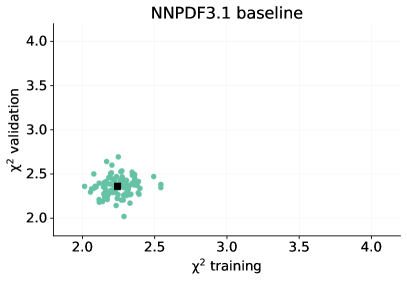
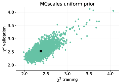
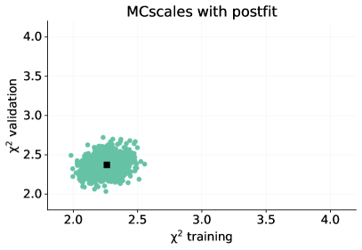
Figure 3.1: The values of the training and validation $\chi^{2}$ per replica for the NNPDF3.1 baseline (top left), the MCscales uniform prior (top right) and the MCscales with postfit set (bottom). The result for each replica is plotted in green, with the mean plotted with a black square.

Fig. 3.1 shows the $\chi^{2}$ to these two data sets plotted for each replica. Three PDF sets are shown: the NNPDF3.1 baseline, the MCscales uniform prior and the same set but after the postfit vetoes have been applied to it. Table 3.1 shows the mean and standard deviation of each of these $\chi^{2}$ distributions. From these we see that the MCscales set with a uniform prior has many more outliers than the other two sets, with these outliers exhibiting a poor agreement with the experimental data. Such replicas drive sizeable increases in the mean and standard deviation of the $\chi^{2}$ distributions versus the other two PDF sets. This confirms the need of the modified selection procedure discussed in Sect. 2.2 and explicitly given in Eq. (2.6) rather than the one of Eq. (2.5). Once it has been applied, the MCscales set exhibits very similar behaviour to the baseline NNPDF3.1 set, with the scatter plot and the means and standard deviations being totally comparable.

		Baseline	MCscales uniform prior	MCscales with postfit
$\chi^{2}_{\text{training}}$	mean	2.24	2.38	2.26
	std	0.10	0.19	0.10
$\chi^{2}_{\text{validation}}$	mean	2.36	2.53	2.37
	std	0.11	0.22	0.11

Table 3.1: The mean values and standard deviations of the $\chi^{2}$ to the training and validation data sets, computed from the distributions shown in Fig. 3.1. Note that all $\chi^{2}$ values are per data point.

3.2 Distributions over scales

We now turn our attention to how postfit affects the distribution of the scale combinations in the MCscales set. To begin, in Fig. 3.2 we look at the distribution of each of the scales over replicas by comparing the flat distribution corresponding to the MCscales uniform prior to the distribution after postfit selection. We observe that the distribution changes significantly after applying postfit. We observe a strong preference for the central factorisation scale, $k_{f}=1$. We also see that postfit affects each process in a different way. As far as DIS CC or jets are concerned, the data do not prefer any of the renormalisation scale choices, while for the DIS NC the data strongly prefer $k_{r}=2$. DY data tend to prefer a lower value of the renormalisation scale, with $k_{r}=1/2$ being favoured over the other scale options, while the top data tends to disfavour $k_{r}=2$. The differences over scale choices are driven by the $\chi^{2}$ postfit criterion Eq. 2.5, with little discernible correlation between the positivity and arclength criteria with the choice of scale combination.

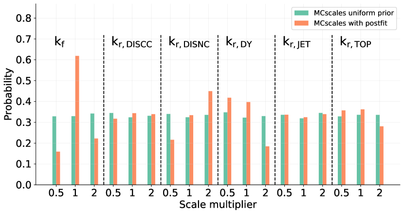
Figure 3.2: The distribution of PDF replicas over each of the scales in two cases: in green for the MCscales uniform prior and in orange for the distribution after postfit.

It is instructive to look at the distribution over scales in more fine-grained detail by studying the effect on the renormalisation scale for each process in addition to the factorisation scale. Since we assign one renormalisation scale to each process and we vary the factorisation scale and the renormalisation scales independently, there are nine scale combinations per process and therefore there are 45 scale combinations in total. The percentage of PDF replicas with a given scale combination after postfit are shown in Fig. 3.3. We observe that across all processes the central value of the factorisation scale is favoured by the data. In the case of DIS CC, the central value of the renormalisation scale is also favoured, while in the case of DIS NC a larger value is favoured by the data. As far as DY data are concerned, a lower value of the renormalisation scale is favoured by the data independently of the factorisation scale value. Interestingly the survival percentage is larger for $(k_{f},k_{r}^{\rm(DY)})=(0.5,0.5)$ and $(k_{f},k_{r}^{\rm(DY)})=(0.5,2.0)$ than for $(k_{f},k_{r}^{\rm(DY)})=(1.0,0.5)$ and $(k_{f},k_{r}^{\rm(DY)})=(1.0,2.0)$. This compensates the larger survival percentage for $(k_{f},k_{r}^{\rm(DY)})=(1.0,1.0)$ compared to $(k_{f},k_{r}^{\rm(DY)})=(1.0,0.5)$ and makes $k_{r}^{\rm(DY)}=0.5$ the scale favoured by data. In the case of inclusive jet data, there is basically no dependence on the renormalisation scale, while in the case of top data a larger value of the renormalisation scale is clearly disfavoured by the data.

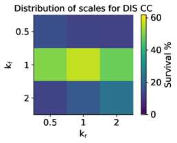
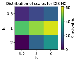
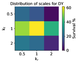
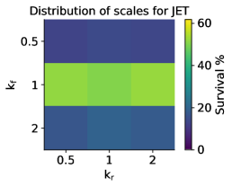
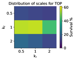
Figure 3.3: The percentage of surviving replicas after postfit relative to the MCscales uniform prior for all scale combinations.

We see that postfit has a strong impact on the distribution. As we saw in Fig. 3.2, $k_{f}=1$ is preferred to the non-central values. We also observe that the most common scale combination after postfit has been applied is not $(k_{f},k_{r})=(1,1)$ for each process, as might be expected. A summary of the favourite scale combinations is given in Table 3.2. In particular, we see that values of $(1,2)$ and $(1,\frac{1}{2})$ are preferred for the DIS NC and jets data, respectively, while the other processes display a better agreement with the data once central scales are selected.

Scale multipliers	Process	Preferred values
$(k_{f},k_{r})$	DIS CC	$(1,1)$
	DIS NC	$(1,2)$
	DY	$(1,1)$
	Jets	$(1,\frac{1}{2})$
	Top	$(1,1)$

Table 3.2: The preferred scale combination for each process, calculated from the distributions given in Fig. 3.3.

3.3 Impact on PDFs

Since we have information on the scales used to generate each replica, we can study how different scale choices affect the PDFs and their fit quality. Fig 3.4 shows the 823 PDF replicas of the MCscales with postfit set for the gluon at $Q=10$ GeV. Each plot shows the same replicas, while they are coloured differently in each panel according to the combination of scales that were used to generate them. This is shown for two different processes: DIS CC (left panel) and DY (right panel). Here we see that for each case, a scale of $k_{f}=1/2$ (the red, blue and green curves) leads to a diminution of the gluon in the region $10^{-3}\lesssim x\lesssim 0.1$ and to an increase in the region $x\gtrapprox 0.1$. On the other hand, the replicas generated with $k_{f}=2$ (the brown, pink and grey curves) yield a similar gluon in the central-$x$ region but increase it for $x\gtrapprox 0.1$. A very similar behaviour is observed for all of the five processes included in the fit. Interestingly, for DIS NC, the scale combination $(k_{f},\,k_{r})=(2,\,0.5)$ also leads to diminution of the gluon, which is not seen for any other process.

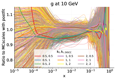
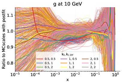
Figure 3.4: PDF replicas of the MCscales with postfit set, for the gluon at $Q=10$ GeV. Each replica is coloured according to its scale choice, where the numbers in the legend correspond to ($k_{f},\,k_{r}$), where $k_{r}$ corresponds to the renormalisation scale for the DIS CC predictions (left panel) or to the one for the DY predictions (right panel). The colouring of the scales is done according to the scales of two different processes included in the fit: the left-hand plot shows the values of the scales for DIS CC and the right-hand plot shows them for DY. The bold lines indicate the average over all replicas for the corresponding scale choice. The plot is normalised to the central replica so that deviations from the central value are shown.

We now study the effect of the scale uncertainties at the level of the PDFs. Fig 3.5 compares the NNPDF3.1 baseline with the MCscales uniform prior set and the MCscales with postfit set. The gluon and the singlet PDFs are displayed along with their 68% C.L. error bands at $Q=10$ GeV. The plots are normalised to the NNPDF3.1 baseline so its central values sit along the $x$-axes. We see that including scale variations in the PDF sets, as is done in the MCscales PDF sets, leads to increased PDF uncertainties, as we would expect. In the $x\in[10^{-4}-10^{-2}]$ region the uncertainty broadening is much stronger for the singlet PDFs than for the gluon PDF. At very small $x$, $x\lessapprox 10^{-4}$ this effect seems to generally be most pronounced, especially for the MCscales uniform prior. We see further that the uniform prior set leads to a general enhancement of the singlet PDFs, while for the gluon PDF the effect is much less marked. However in both cases, after postfit has been applied to the MCscales set based on an uniform prior, the general enhancement is no longer present and the increase in PDF uncertainties tends to become more symmetric.

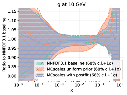
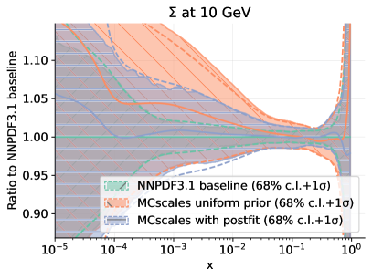
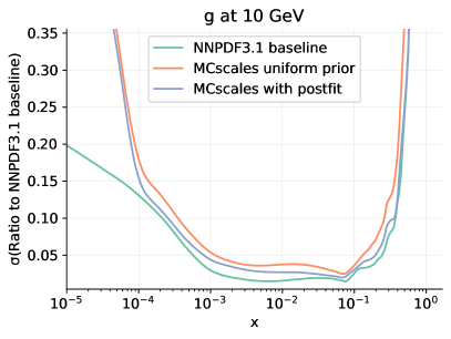
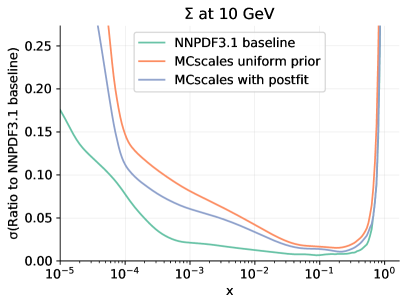
Figure 3.5: Top: plots of the gluon (left) and singlet $\Sigma$ (right) PDFs at $Q=10$ GeV, where NNPDF3.1 baseline (green) is compared to MCscales uniform prior (orange) and the same fit with after postfit (blue). Bottom: The 1$\sigma$ PDF uncertainties, normalised to the central value of the NNPDF3.1 baseline PDF.

Comparing the NNPDF3.1 baseline and the MCscales with postfit set, we see the effect of scale variations once outliers have been sensibly removed. For each flavour the PDFs are compatible within uncertainties, with any shift in the central value induced by scale variations within the uncertainties of the NNPDF3.1 baseline. The shift in the central value appears to be most prominent in the data region for the gluon, where part of the reduction in the gluon PDF observed for the MCscales PDFs without postfit remains after their application.

A discussion concerning the comparison with the PDFs obtained in Refs. AbdulKhalek:2019bux ; AbdulKhalek:2019ihb using the theory covariance matrix approach is given in Appendix 5. Note that the comparison at the level of PDFs does not necessarily reflect the comparison of theory uncertainties at the level of observables. The predictions obtained by matching the scales in the MCscales PDF sets with those in the partonic cross section will have a comparable or even smaller theory uncertainty due to the effect of the correlations between scales. This will be discussed explicitly in Sect. 6 and in Appendix 5.

3.4 Non-uniform models for the prior sampling

So far we have illustrated the results that can be obtained with the MCscales methodology using the simplest option for the prior probability, i. e. a uniform probability distribution over all scale multipliers contained in the set $\Omega$, Eq. (2.2).

Of course, more involved models for the prior probability can be considered. In Appendix A we present a more general model for the prior probability which can be tuned according to the user’s assumptions on the correlation between processes.

In this section, we limit ourselves to study the simplest non-uniform prior probabilities based on the selection of a subset of scale multipliers in $\Omega$. Those correspond to the scales multipliers that are used in the usual the 7-points and 5-points envelope prescriptions. This study will allow us to assess how the MCscales PDF sets behave as the prior probability spans a lower number of scale combinations.

We start by reminding the reader how the scale multipliers are chosen in the n-point prescription. The 7-pts envelope prescription is the most commonly adopted option in phenomenological studies. The multipliers $k_{f}$ and $k_{r_{p}}$ are varied by a factor of two about the central choice while ensuring that 1/2 $\leq k_{f}/k_{r_{p}}\leq$ 2.

$$\Omega|_{\rm 7pts}=\{(\xi_{f},\xi_{1},\ldots,\xi_{N_{\text{p}}})\;\forall\;\xi_{f},\xi_{1},\ldots,\xi_{N_{\text{p}}}\in\Xi\Big{|}\frac{1}{2}\leq\frac{\xi_{f}}{\xi_{p}}\leq 2\}\ .$$ (3.1)

We can also consider the 5-pts prescription where multipliers are obtained by varying $k_{f}$ up and down by a factor of 2 while keeping $k_{r_{p}}=1$ and vice versa, namely

$$\Omega|_{\rm 5pts}=\{(\xi_{f},\xi_{1},\ldots,\xi_{N_{\text{p}}})\;\forall\;\xi_{f},\xi_{1},\ldots,\xi_{N_{\text{p}}}\in\Xi\Big{|}\xi_{f}=1\land\xi_{p}\in\Xi\lor\xi_{p}=1\land\xi_{f}\in\Xi\forall p=1,\ldots,N_{p}\}\ .$$ (3.2)

The MCscales-7pts, MCscales-5pts and PDF sets presented in this section are obtained by starting from the non-uniform priors described in $\Omega|_{\rm 7pts}$, $\Omega|_{\rm 5pts}$ and applying the postfit criteria spelled out in Sect. 2.2

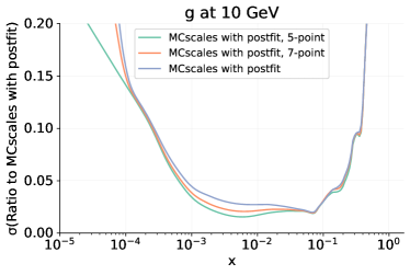
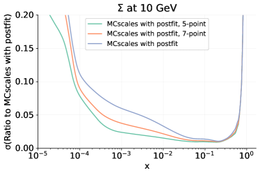
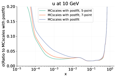
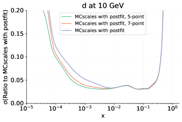
Figure 3.6: Plots of the relative uncertainties of the gluon (top left), singlet $\Sigma$ (top right), up (bottom left) and down (bottom right) PDFs at $Q=10$ GeV once the prior probability is chosen according to the subset of scale choices defined in Eq. (2.2) (blue curves), (3.1) (orange curves) or (3.2) (green curves).

Given that the central value of the sets we explore in this section is very similar to the central value of the MCscales set obtained with a uniform prior, we focus on the relative uncertainties of the PDFs determined by starting from a prior that includes the subsets of points defined in (3.1) and (3.2) behave. In Fig. 3.6 we observe that uncertainties are comparable in the medium to large-$x$ region, for $x\gtrsim 10^{-2}$, while the moderate- to small-$x$ region is more affected, especially for the quarks. Indeed the relative uncertainty decreases by about a factor of 2 for $x\sim 10^{-3}$. This may be associated with the fact that the (2,1/2) and (1/2,2) combinations have a stronger pull to the gluon and singlet evolution, and thus yield replicas that span a broader range in the small-$x$ region.

4 Cross section computation with MCscales PDFs

Here we describe the machinery to produce phenomenological results with MCscales PDFs. Because the scale variation information used to produce each PDF replica is stored, users have the ability to match the scale variations in the partonic cross section of interest with those used in the theoretical predictions in the PDF fit, thus attaining theory predictions with fully consistent scale variations. These steps are laid out in Sect. 4.1. Additionally, in Sect. 4.2 we define two other ways to compute predictions which make use of a more limited amount of information, for the purpose of assessing the effect of fully matching the scales.

4.1 Theoretical predictions with matched scales

The Monte Carlo formalism typically used in the NNPDF PDF sets requires computing a sample of theory predictions for a given partonic cross section $\hat{\sigma}$, from the set of $N$ PDF replicas $\{f_{n}\}$ with $n=1,\ldots,N$

$$\left\{\sigma_{n}=\hat{\sigma}\otimes f_{n}\ \,\forall\,n=1,\ldots,N\right\}\,,$$ (4.1)

where the symbol $\otimes$ schematically represents the Mellin convolution between each PDF replica set and the partonic cross section for a given process. Statistics over this sample is then applied to extract information on the PDF dependence of the observable under inspection; notably the central value of the theory prediction for that given observable is taken to be the average of the $\{\sigma_{n}\}$ sample and the PDF uncertainty is taken to be its standard deviation.

Our present work allows this method to be extended to include information on the combined PDF and scale uncertainty to determine the total (i e. the PDF+scale) theoretical uncertainty associated with a given theoretical prediction. As described in Sect. 2, we store the information on the scale variations used in the theory predictions for the input data of each replica, namely the factorisation scale and five distinct renormalisation scales, one for each of the five physical processes into which we split our input data set. This makes it possible to match the factorisation and renormalisation scale variations of a given cross section prediction with those used in the determination of the PDF set. We distinguish between two cases, depending on the nature of the process under inspection: the first case is when the process is one of the five processes included in the PDF fit, and the second is when instead we consider a new process not present in the fit. We now consider each in turn.

In the first case, both the factorisation and renormalisation scale variations can be matched: the partonic cross section for the process $p$, $\hat{\sigma}_{p}(k_{f},k_{r_{p}})$ (where we now note explicitly both the index of the process and the dependence on the scale multipliers) can be computed with the nine scale variations, yielding the nine partonic cross sections,

$$\left\{\hat{\sigma}_{p}(k_{f},k_{r_{p}})\,\,\forall\,k_{f},k_{r_{p}}\in\Xi\right\}\ .$$ (4.2)

The scale variations of (4.2) can be associated with variation in the replicas of the MCscales PDF set to yield a sample that matches both the factorization and the renormalization scale for a given process in the input PDF set and in the computation of the partonic cross section. The sample is built as

$$\left\{\sigma_{n}=\hat{\sigma}_{p}(k_{f}^{(n)},k_{r_{p}}^{(n)})\otimes f_{n}(k_{f}^{(n)},k_{r_{p}}^{(n)})\ \,\,\forall\,n=1,\ldots,N\right\}\ ,$$ (4.3)

where $k_{f}^{(n)}$ is the factorisation scale multiplier associated with replica $n$, and $k_{r_{p}}^{(n)}$ is the renormalisation scale multiplier associated with replica $n$ for process $p$, and where we have left implicit the dependence of $f_{n}$ on the scale multipliers associated with the renormalization scale of the other $(N_{p}-1)$ processes. The sample of replicas constructed as in Eq. (4.3) now contains the information both on the scales used in the fit yielding each individual PDF replica and on the scales used in the computation of the partonic cross section for each PDF replica. Crucially, computing the standard deviation of the sample in Eq. (4.3) results in a total theory uncertainty, including the experimental PDF uncertainty and the scale uncertainty. The scale uncertainty comprises both the scale uncertainty in the partonic cross section and the one in the PDFs, with the correlations fully accounted.

We now address the situation in which a prediction is being made for a process that is not among the input data sets in the PDF analysis, such as Higgs production. In this case we indicate the renormalisation scale associated with the Higgs production partonic cross section as $k_{r}$ (rather than $k_{r_{p}}$ as we do when the process is one of those included in a PDF fit). Here only the factorisation scale variations can be matched, while there is no process to match the renormalisation scale variations with. In this case one can instead construct a sample of size $3N$ by first setting the renormalization scale for the process not included in the PDF fit to 1/2 and convoluting the partonic cross section with all replicas in the MCscales set by matching the factorization scale in the computation of the partonic cross section with those in the PDF set. Subsequently, the same matched convolution is done by setting the renormalization scale for the process to 1 and then to 2. The set is built as

$$\begin{split}\left\{\sigma_{n}=\hat{\sigma}_{p}\left(k_{f}^{(n)},k_{r}^{(n)}=\frac{1}{2}\right)\otimes f_{n}(k_{f}^{(n)})\ \,\,\forall\,n=1,\ldots,N\right\}\cup\\ \left\{\sigma_{n}=\hat{\sigma}_{p}\left(k_{f}^{(n)},k_{r}^{(n)}=1\right)\otimes f_{n}(k_{f}^{(n)})\ \,\,\forall\,n=1,\ldots,N\right\}\cup\\ \left\{\sigma_{n}=\hat{\sigma}_{p}\left(k_{f}^{(n)},k_{r}^{(n)}=2\right)\otimes f_{n}(k_{f}^{(n)})\ \,\,\forall\,n=1,\ldots,N\right\}\,.\end{split}$$ (4.4)

The resulting sample will weight the factorisation scale variation as in the input PDF and will assume that the three renormalisation scale variations are equally likely, as per our prior assumption in Sect. 3.

Regardless of how the sample is constructed, the central value $\bar{\sigma}$ and the total theory uncertainty $\Delta$ including both the total PDF uncertainty and the scale uncertainty of the partonic cross section can be obtained by computing the mean and standard deviation of the sample:

$$\bar{\sigma}^{\rm(corr)}=\left\langle\sigma_{n}\right\rangle\ ,$$ (4.5)

$$\Delta^{\rm(corr)}=\text{std}(\sigma_{n})\ ,$$ (4.6)

where the set $\{\sigma_{n}\}$ has been obtained with either Eq. (4.3) or Eq. (4.4), depending on whether the process is included or not in a PDF fit.

4.2 Theoretical predictions using less information

In order to study the effect of employing MCscales PDFs using the full information on the scale correlations, as described in Sect. 4.1, here we define two other ways to compute cross sections, which utilise less of the available information.

The first method mimics what happens when one estimates theory uncertainties using conventional PDFs; that is, PDFs that do not include any scale variation uncertainty. In this case, rather than working with an MCscales PDF set, we use the subset of the $N_{c}=192$ PDF replicas for which all factorisation and renormalisation scales are set to their central values. To compute the PDF uncertainty, we follow the standard approach of computing a set of $n$ replicas of the cross sections computed for the central PDF set

$$\left\{\sigma_{n}^{(c)}=\hat{\sigma}(k_{f}=1,k_{r_{p}}=1)\otimes f^{(c)}_{n},\ \,\,\forall\,n=1,\ldots,N_{c}\right\}\ ,$$ (4.7)

where $(c)$ stands for “central” and the replicas in $\left\{f^{(c)}_{n}\right\}$ are all obtained with the central values of the scales. The central value of the theory prediction is given by

$$\bar{\sigma}^{(c)}=\hat{\sigma}(k_{f}=1,k_{r_{p}}=1)\otimes f^{(c)}_{0},$$ (4.8)

where $f^{(c)}_{0}$ is the central replica (replica 0) of the $\{f_{n}^{(c)}\}$ subset of the MCscales set. The PDF-only uncertainty is given by

$$\Delta^{{\rm PDF}_{\rm exp}}={\rm std}(\sigma_{n}^{(c)})\ ,$$ (4.9)

where the suffix ${\tt exp}$ indicates a PDF uncertainty that only propagates the experimental uncertainty of the data included in a fit.

Next we define the set of nine cross sections computed over all nine combinations as in Eq. (4.2) and we convolve them with $f^{(c)}_{0}$, yielding nine values of the cross section for the process under consideration

$$\sigma_{0,i}^{(c)}=f^{(c)}_{0}\otimes\hat{\sigma}(k_{f},k_{r})\ ,\qquad i=1,\ldots,9,$$ (4.10)

where $i$ indicates one of the 9 possible combinations of $\{k_{f},k_{r}\}\in\Xi$, which will be used to compute an estimate of the scale uncertainty. In order to maintain an equivalence with the computation using the MCscales model as described in Sect. 4.1, we weight each scale variation by the same amount as in the original MCscales PDF set (see Fig. 3.3). The weight for each of the nine contributions is

$$w_{i}=\frac{N_{i}}{N}$$ (4.11)

where $N_{i}$ counts the number of replicas in the MCscales with relevant scale multipliers set to one of the 9 elements of  (4.2). The associated weighted variance is given by

$$(\Delta^{\rm scale})^{2}=\frac{1}{1-\sum_{i=1}^{9}w_{i}^{2}}\sum_{i=1}^{9}w_{i}(\sigma_{0,i}^{\rm(c)}-\bar{\sigma}^{\rm(c)})^{2}\,,$$ (4.12)

where

$$\bar{\sigma}^{\rm(c)}=\sum_{i=1}^{9}w_{i}\sigma_{0,i}^{\rm(c)}\,.$$ (4.13)

Thus, the total theory uncertainty $\Delta^{\rm(c)}$ including only PDF experimental uncertainty and the scale variation in the partonic cross section in an uncorrelated way is given by

$$\Delta^{\rm(c)}=\sqrt{(\Delta^{{\rm PDF}_{\rm exp}})^{2}+(\Delta^{\rm scale})^{2}}\ .$$ (4.14)

The second alternative method involves combining the scale variation in the partonic cross section with that in the MCscales PDF in an uncorrelated way. This will allow us to gauge the loss of accuracy incurred in when adding scale uncertainties in PDFs but no mechanism to match them to the partonic cross sections, as was done in Ref. AbdulKhalek:2019ihb . The PDF uncertainty here is composed of both the experimental and the scale variation components, to which we add a component to account for the scale uncertainty in the partonic cross section. We convolve all replicas in the MCscales set with the hard cross section using unmatched, central scales

$$\left\{\sigma_{n}^{\rm(uncorr)}=\hat{\sigma}_{p}(k_{f}=1,k_{r_{p}}=1)\otimes f_{n}(k_{f}^{(n)},k_{r_{p}}^{(n)})\ \,\,\forall\,n=1,\ldots,N\right\}\ .$$ (4.15)

The central value for the prediction is given by

$$\bar{\sigma}^{\rm(uncorr)}=\,\left\langle\sigma_{n}^{\rm(uncorr)}\right\rangle\ .$$ (4.16)

In order to obtain a component of the uncertainty accounting for the experimental and scale uncertainties in the PDF fit, we compute

$$\Delta^{{\rm PDF}_{\rm exp+scale}}={\rm std}(\sigma_{n}^{\rm(uncorr)})\ ,$$ (4.17)

to which we add a component to account for the scale uncertainty in the hard cross section, $\Delta^{\rm scale}$ defined as in Eq. (4.12). Finally, the total uncertainty including both the PDF uncertainty (experimental and scale) and the scale uncertainty of the partonic cross section in an uncorrelated way is given by

$$\Delta^{\rm(uncorr)}=\sqrt{(\Delta^{{\rm PDF}_{\rm exp+scale}})^{2}\,+\,(\Delta^{\rm scale})^{2}}\,.$$ (4.18)

In Sect. 6 we will explore in details how the estimate of theory uncertainty in a NLO prediction changes depending on whether one uses the full information on scale variations in the PDF input set and its correlation with the scales in the partonic cross sections or not.

5 Comparison with the theory covariance matrix approaches

As we mentioned in Sect. 1, the methodology presented in this work is based on a different principle as compared to the approach based on the construction of a theoretical covariance matrix  AbdulKhalek:2019bux ; AbdulKhalek:2019ihb . In the latter, a covariance matrix is postulated, based on differences in predictions with varying scale choices, and it is added up to the experimental covariance matrix, both in the sampling of the Monte Carlo replicas and in the figure of merit used in the fit itself. The predicted quantities, on which the PDF determination is based, are not dependent on individual scales but rather a marginalisation of the distribution of scales (see Eq. (2.9) of Ref. AbdulKhalek:2019ihb and surrounding discussion). In the notation of Sects. 2 and 4, this would roughly correspond to

$$\sum_{\omega\in\Omega}\hat{\sigma}_{p}(\omega)\otimes f(\omega)P(\omega)\ ,$$ (5.1)

where the dependence on $\hat{\sigma}$ is only through the relevant scale variations $k_{f}$ and $k_{r_{p}}$ in $\omega$.

In the MCscales approach presented in this paper, the scales entering a PDF fit are treated as free parameters of the fixed-order theory. Thus, the experimental uncertainty of the data and of the scales uncertainty associated to theory predictions are both propagated onto the PDF uncertainties via a Monte Carlo sampling in the joint space of experimental data and scale variations (the latter subject to the constraints spelled out in Sect. 2), which implies producing independent determinations for each $\hat{\sigma}_{p}(\omega)\otimes f(\omega),\forall\omega\in\Omega$.

We compare the results obtained starting from a uniform prior probability for the scales, to those obtained with the theory covariance matrix approach. Among the various possibilities described in Ref. AbdulKhalek:2019ihb , we compare our results to those obtained with the 9-point prescription, in which all scale variations in $\Omega$ are considered.

The MCscales approach might look slightly more similar to the approach explored in Sect. 6 of Ref. AbdulKhalek:2019ihb , in which the theory covariance matrix is included only in the data generation but not in the $\chi^{2}$ used as a figure of merit in the fit. The corresponding PDF set is called NNPDF31_nlo_as_0118_scalecov_9pt_sampl. In that case, increased uncertainties and a worse fit quality are obtained, since the data replica fluctuations are wider due to the MHOUs, but this is not accounted for in the $\chi^{2}$ minimisation. As a result, the increase in uncertainty due to the inclusion of MHOU in the sampling is not compensated by a rebalancing of the datasets and a reduction of the scale uncertainty obtained via the inclusion of MHOU in the fit. However, one should be careful in comparing the two approaches. Indeed, while in the theory covariance matrix approach the predictions $T_{i}^{(n)}$ that enter the computation of the $\chi^{2}$, Eq. (2.4), are computed by using the central scales ($k_{f}=k_{r_{p}}=1$), in the MCscales approach, the theoretical predictions are computed with the factorisation and renormalisation scales matched to the element $\omega$ of the sampling of the replicas ($k_{f}=\xi_{f},k_{r_{p}}=\xi_{r_{p}},p=1,...,N_{p}$). This has the effect of approximating the scale varied predictions of the data in the fit to the corresponding experimental values.

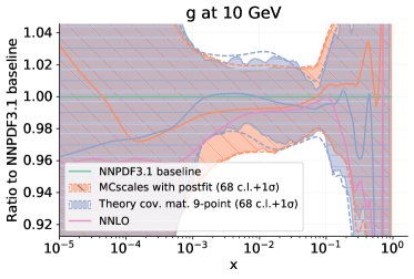
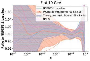
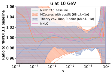
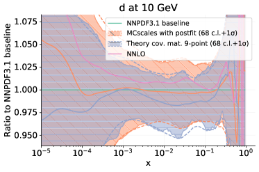
Figure 5.1: Plots of the gluon (top left), singlet $\Sigma$ (top right), up (bottom left) and down (bottom right) PDFs at $Q=10$ GeV, where the PDF set obtained in Ref. AbdulKhalek:2019ihb by using the theory covariance matrix built with a 9-point prescription (NNPDF31_nlo_as_0118_scalecov_9pt) (blue) is compared to the PDF set obtained with the MCscales approach starting from a uniform prior and after postfit (MCscales with postfit) (orange). The central NNLO baseline set (NNPDF31_nlo_as_0118) is also displayed, in pink. The PDFs are normalised to the central value of the NLO baseline set (NNPDF31_nlo_as_0118, green). We note that cross section computations using the MCscales sets should use matched scale variations in the partonic cross section (see Sect. 4), which heavily limits the interpretability of this comparison.

We compare the default results of both approaches, namely the PDF set obtained by using the 9-point theory covariance matrix both in the sampling and in the fitting, the NNPDF31_nlo_as_0118_scalecov_9pt set, and the PDF set that is obtained with the MCscales approach starting from a uniform prior and after postfit MCscales with postfit. These sets are compared in Fig. 5.1, by displaying the gluon, singlet, up and down-quark PDFs at the scale $Q=10$ GeV. The plots are normalised to the central value of the NNPDF3.1 NLO baseline PDFs. We observe that, as far as the gluon and the singlet are concerned, the PDF uncertainties of the MCscales set are only moderately larger than those obtained with a 9-point theory covariance matrix. The larger increase in uncertainty is observed in the up-quark PDF, especially in the medium-small-$x$ region $x\in[10^{-4},10^{-2}]$. We expect the uncertainty increase in PDFs to be compensated, when computing partonic cross sections, and even even result in smaller uncertainties, when correctly accounting for the correlations in scale variations in PDFs and partonic cross sections, as we will show explicitly in what follows. The central values of the two sets are compatible within $1\sigma$ error band, with the MCscales set yielding harder PDFs at small-$x$. It is interesting to observe that the small-$x$ behaviour reminds the one observed in Ref. McGowan:2022nag , although our study is conducted at NLO rather than NNLO. The shift in the central values that we observe here is much less dramatic than in McGowan:2022nag , given the somewhat different approach that we adopt: rather than having the data determine the scales in the theoretical predictions and their uncertainties by treating them as nuisance parameters to be constrained by the fit, here we only use the data to discard the scale combination that yield a very poor agreement between theory predictions and experimental data.

We emphasise that the cross section predictions that use MCscales PDFs are intended to use matched scale variations in the partonic cross sections. As a result the PDFs are not directly comparable to those in the theory covariance matrix approach, where PDFs are to be convoluted with partonic cross sections using central scales only. This is an important caveat to the PDF plots presented so far. To illustrate this point, in Fig. 5.2 we show the comparison between the experimental data and the theoretical predictions for a reduced neutral current DIS cross section measured at HERA Abramowicz:1900rp and for the charged current cross section H1:2018flt , where the theoretical predictions and their total theoretical uncertainty (including both the scale uncertainty in the partonic cross sections and the PDF uncertainty - in turn including both the experimental and the scale uncertainties in a PDF fit) have been computed using the PDF set obtained with a 9-pts theory covariance matrix and with the MCscales set. The uncertainty bands for the theory covariance matrix have been obtained using Eq. (8.3) of Ref. AbdulKhalek:2019ihb , which is analogous to the uncorrelated prescription presented in Sect. 4.2 while the MCscales predictions use Eq. 4.3.

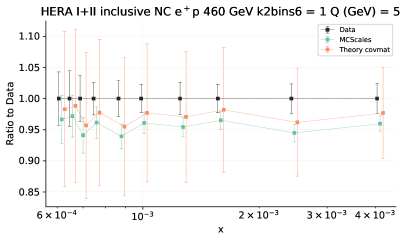
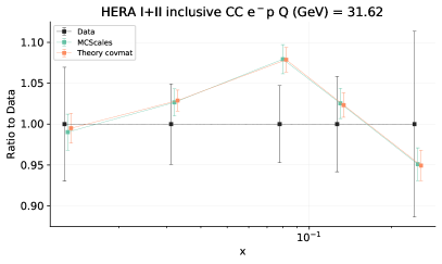
Figure 5.2: Ratio to HERA inclusive neutral current positron-electron cross section data Abramowicz:1900rp (left) and HERA inclusive charged current data H1:2018flt (right) of the theoretical predictions obtained with MCscales and theory covariance matrix approaches to the respective data.

We observe that the MCscales uncertainties on the cross sections can indeed be smaller than those computed with the theory covariance matrix approach, as they account for the correlations of the scales and also due to the postfit selection, but also bigger in cases where the underlying assumptions differ. This illustrates how the comparison at the level of PDFs in Fig. 5.1 might lead to incorrect conclusions with regard to the relative uncertainty in the two approaches.

An alternative procedure to disentangle the effect of individual scale variations and study the correlation between theory uncertainties in PDF fits and predictions made with such PDF sets was presented in Ref. Ball:2021icz . The method is based on the theory covariance matrix formalism. However, rather than producing a PDF fit by computing the marginalised predictions (as it is done in Eq. 5.1) it interprets the difference between data and theory predictions computed with the central scales as the shifts in the predictions derived from the theory covariance matrix (insofar those are projected into the relevant subspace, as explained in detail in Ref. Ball:2021icz ). By contrast, the MCscales procedure discussed here operates directly on the scale parameters, which are determined for each replica by the prior distribution and remain unchanged during the fit. As a result, the post-fit replica selection in MCscales has a weaker effect in terms of constraining the scales. On the other hand the MCscales procedure does not assume that the differences between data and predictions come exclusively from the theory uncertainties. Another difference in the two approaches comes from the fact that in the MCscales procedure both the predictions used in the fit and those computed with the resulting PDFs are matched exactly, thereby avoiding any assumptions on the Gaussianity and smallness of the theory corrections. Such hypotheses do not necessarily apply to all data. Indeed, in Sect. 3.2, we show that scale variations have a large impact on the fit quality and are therefore comparable to experimental uncertainties. Secondly, the MCscales procedure provides direct access to the scale parameters, allowing external users to study and even tune the scale dependence of the resulting fit. Furthermore, given that the procedure in Ref. Ball:2021icz is based on the results of a pre-existing PDF fit scale shifts, it might be subject to the problems pointed out in Ref. Forte:2020pyp for the equivalent case of fitting the strong coupling constant. The result in this case would not be the same as those of a simultaneous fit of PDFs and scale shifts.

In order to understand how the differences in the approaches affect the results, it would be very interesting to implement the two procedures in the computation of the LHC observables that we will present in Sect. 6, and compare the results in all cases. We leave this to a future study, in which both methodologies may take advantage of the more modern NNPDF4.0 PDF set nnpdf40 and of the theory pipeline implementation presented in Barontini:2023vmr .

6 Application to phenomenology

In this section we compute reference LHC standard candles with the NLO PDF sets from our Monte Carlo samplings presented in Sect. 3 and the definitions given in Sect. 4. Most importantly, for the first time we will be able to assess the importance of the correlation between the scale variation in the computation of the partonic cross sections and the scale variation in the PDF fit as well as the impact of their double counting.

For our assessment to be meaningful, it is important that the partonic cross sections are computed at the same perturbative order as the observables included in a PDF fit. While this requirement does not hold if correlations are neglected, as in Ref. AbdulKhalek:2019ihb , once correlations are fully taken into account according to Eq. (4.3) it is important that the scale variations are performed at the same perturbative order. For this reason, we will only consider the NLO computaton of key processes at the LHC. Once a PDF set including scale variation will be available at NNLO, our analysis can be straightforwardly extended.

In our two-fold investigation, we will first consider the Higgs boson production in gluon-fusion and in vector-boson fusion, as examples of processes that are not included in a PDF fit, where the effect of correlations is expected to be milder. We then consider top quark pair production and the $Z$ and $W$ electroweak gauge boson production, as examples of processes included in a PDF fit, where the effect of correlations is expected to be stronger.

6.1 Higgs production

We start by discussing Higgs production in gluon fusion (ggF) and in vector boson fusion (VBF). These two processes are of direct relevance for the characterisation of the Higgs sector and are both currently known at N³LO accuracy Anastasiou:2015vya ; Anastasiou:2016cez ; Mistlberger:2018etf ; Dreyer:2016oyx . The processes are complementary in two respects. On the one hand, Higgs production in gluon fusion is driven by the gluon-gluon luminosity and its perturbative expansion converges slowly. On the other hand vector boson fusion is driven by the quark- anti-quark luminosity and it exhibits fast perturbative convergence.

In Table 6.1 we present predictions for Higgs production in ggF at the LHC for $\sqrt{s}=$ 13 TeV. Given that we focus on the effect of correlations between the factorisation scale used in the PDF replicas and the factorisation scale used in the partonic cross section, it is important to perform them at the same order, i.e. at NLO. We perform the calculation of ggF at NLO in the rescaled effective theory approximation using ggHiggs Bonvini:2014jma ; Bonvini:2016frm with $\mu_{f}^{0}=\mu_{r}^{0}=m_{H}/2$, with the MCscales with postfit set obtained in this paper. In the first line, we use the fully correlated prescription, Eqs. (4.5) and (4.6), while in the second and third lines we use the prescriptions that use less information, namely the uncorrelated prescription, Eqs. (4.16) and  (4.18), in which the scale uncertainty in the PDFs is combined with the scale uncertainty in the partonic cross section in an uncorrelated way, and finally the prescription in which we ignore scale uncertainty in PDFs, as in Eqs. (4.13) and (4.14). The comparison between the first and the second lines gives us an estimate of the size of correlations between scales and the double-counting of scale variation in the PDFs and in the partonic partonic cross sections, while the comparison between the first two lines and the third gives us an idea on the effect of neglecting scale uncertainty in PDF fits.

Higgs production by gluon fusion at 13 TeV [pb]
	NLO
$\bar{\sigma}^{\rm(corr)}\,\pm\,\Delta^{\rm(corr)}$	38.10 $\pm$ 19.5%
$\bar{\sigma}^{\rm(uncorr)}\,\pm\,\Delta^{\rm(uncorr)}$	37.41 $\pm$ 17.9%
$\bar{\sigma}^{\rm(c)}\,\pm\,\Delta^{\rm(c)}$	37.64 $\pm$ 17.7%

Table 6.1: The central value and the total theoretical uncertainty for the Higgs production cross section by gluon fusion at NLO for $\sqrt{s}=13$ TeV. The settings are indicated in the text. All results are produced with NLO PDFs, and the central values and total theoretical uncertainty are computed according to three different prescriptions. $\Delta^{\rm(corr)}$ is the correlated theoretical uncertainty in which the scale variation in the PDF fit are correlated with the scale variations in the computation of the partonic cross section, Eqs. (4.5) and (4.6). $\Delta^{\rm(uncorr)}$ is the theoretical uncertainty in which the scale variations in the PDF fit are uncorrelated with the scale variations in the computation of the partonic cross section, Eqs. (4.16) and (4.18). $\Delta^{\rm(c)}$ is the total theory uncertainty in which scale uncertainty is included only in the partonic cross section, Eqs. (4.13) and (4.14). The NNLO central value is $46.53$ pb.

We observe that in this case not accounting for the correlation between the factorisation scale variation in the PDFs and the factorisation scale variation in the computation of the Higgs cross section underestimates the theory uncertainty by a non-negligible amount. The total theory uncertainty increases by nearly 2% in absolute value. This finding contradicts the somewhat intuitive statement according to which the computation of the total theory uncertainty in an uncorrelated way is a conservative estimate of theory uncertainties. In this case the correlation between the factorisation scale variation in the PDF fit and those in the computation of ggF Higgs production cross section does increase the total uncertainty, rather than decreasing it. Results are displayed graphically in Fig. 6.1 where, for the NNLO computation, we also show the central value found using NNLO PDFs.

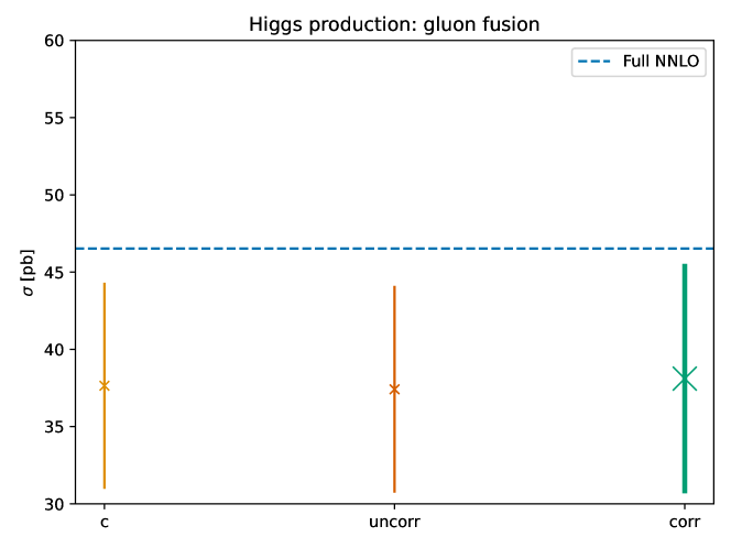
Figure 6.1: NLO total cross sections for the Higgs production cross section by gluon fusion at NLO for $\sqrt{s}=13$ TeV. The uncertainty on each result is the total theoretical uncertainty, which includes both PDF and scale uncertainties according to the three different prescriptions described in the text and in Table 6.1. The NNLO result, which uses the NNLO NNPDF3.1 baseline PDFs, is also displayed.

We observe that the central value of the NLO cross section computed over the MCscales set according to the correlated prescription gets closer to the next perturbative order.

We now turn to Higgs production in vector boson fusion. We perform the NLO calculation using proVBFH-inclusive Cacciari:2015jma with central factorisation and normalisation scales set equal to the squared four-momentum of the vector boson. Results are collected in Table 6.2 and shown in Fig. 6.2. We observe that in this case the inclusion of the correlation between the factorisation scale variations in the Higgs production partonic cross section and those in the PDFs does decrease the scale uncertainty by a non-negligible amount. On the other hand, we also observe that not including the effect of theory uncertainties in PDFs would significantly underestimate theory uncertainties in this process.

Higgs production by virtual boson fusion at 13 TeV [pb]
	NLO
$\bar{\sigma}^{\rm(corr)}\,\pm\,\Delta^{\rm(corr)}$	4.010 $\pm$ 1.77%
$\bar{\sigma}^{\rm(uncorr)}\,\pm\,\Delta^{\rm(uncorr)}$	4.006 $\pm$ 1.97%
$\bar{\sigma}^{\rm(c)}\,\pm\,\Delta^{\rm(c)}$	4.003 $\pm$ 1.15%

Table 6.2: Same as Table 6.1 for the NLO total cross sections for the Higgs production cross section by vector boson fusion at NLO for $\sqrt{s}=13$ TeV. In this case, the NNLO central value is $4.025$ pb.

Results are displayed graphically in Fig. 6.2, in which we see that the uncertainty bands increases once scale uncertainty in PDFs is accounted for, and slightly decreases once correlations are fully taken into account. Also in this case the central value of the NLO cross section computed over the MCscales set according to the correlated prescription gets closer to the next perturbative order.

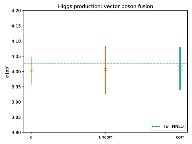
Figure 6.2: The same as Fig. 6.1 but for Higgs production by vector boson fusion at 13 TeV.

6.2 Top pair production

We now turn to the impact of PDF-related scale uncertainty and the effect of the correlations between scale variations in the PDFs and in the partonic cross section by computing the total top-pair production cross section at the LHC at $\sqrt{s}=$ 13 TeV.

Top pair production at 13 TeV [pb]
	NLO
$\bar{\sigma}^{\rm(corr)}\,\pm\,\Delta^{\rm(corr)}$	725.6 $\pm$ 6.98%
$\bar{\sigma}^{\rm(uncorr)}\,\pm\,\Delta^{\rm(uncorr)}$	718.8 $\pm$ 6.59%
$\bar{\sigma}^{\rm(c)}\,\pm\,\Delta^{\rm(c)}$	718.4 $\pm$ 6.38%

Table 6.3: Same as Table 6.1 for the NLO total cross sections for the top pair production cross section NLO for $\sqrt{s}=13$ TeV. In this case, the NNLO central value is $786.0$ pb.

In Table 6.3 we collect, using the same format as Table 6.1 , the predictions for the top-quark pair-production cross-sections at $\sqrt{s}$ = 13 TeV obtained using the top++ code Czakon:2011xx and setting the central scales to $\mu_{f}^{0}=\mu_{f}^{0}=m_{t}=$ 173.3 GeV. The results are also displayed in Fig. 6.3, where again for at NNLO we also show the result obtained using NNPDF3.1 NNLO baseline PDFs.

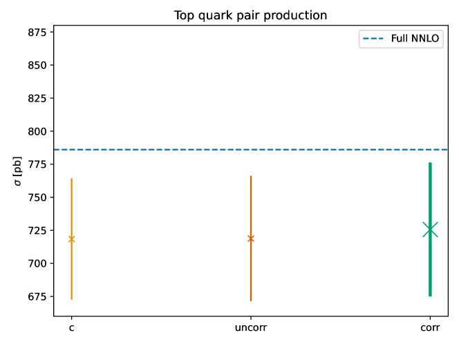
Figure 6.3: The same as Fig. 6.1 but for the top quark pair production at $\sqrt{s}=13$ TeV.

We observe that in this case the effect of the correlation is almost negligible. As in the case of Higg production via gluon fusion, the correlation is negative and its inclusion increases the total theoretical uncertainty, although by a small amount in this case. This is in contrast with what is observed in Ref. Ball:2021icz , possibly due to a different methodology to compute the matched predictions. In this paper we simply match the subsets of PDF replicas to the partonic cross section that set matching values of scale, while in  Ball:2021icz the theoretical predictions are computed using different definitions of the theory covariance matrix and a direct comparison is not straightforward.

6.3 Vector boson production

We finally turn to gauge boson production, for which we obtain predictions using FEWZ Li:2012wna ; Gavin:2012sy ; Gavin:2010az . For the theoretical predictions for inclusive $W$ and $Z$ production cross sections at $\sqrt{s}$ = 13 TeV, we adopt realistic kinematic cuts similar to those applied by ATLAS and CMS. The fiducial phase space for the $W^{\pm}$ cross-section is defined by requiring $p_{T}^{l}\geq$ 25 GeV and $\eta_{l}\leq$ 2.5 for the charged lepton transverse momentum and pseudo-rapidity and a missing energy from the neutrino of $p_{T}^{\nu}\geq$ 25 GeV. In the case of $Z$ production, we require $p_{T}^{l}\geq$ 25 GeV and $|\eta_{l}|\leq$ 2.5 for the charged leptons transverse momentum and rapidity and 66 $\leq m_{ll}\leq$ 116 GeV for the di-lepton invariant mass.

Vector boson production at LHC 13 TeV [pb]
	Z (NLO)	$W^{+}$ (NLO)	$W^{-}$ (NLO)
$\bar{\sigma}^{\rm(corr)}\,\pm\,\Delta^{\rm(corr)}$	785.8 $\pm$2.40%	4615.3$\pm$2.14%	3529.7$\pm$2.15%
$\bar{\sigma}^{\rm(uncorr)}\,\pm\,\Delta^{\rm(uncorr)}$	784.1$\pm$4.17%	4603.86$\pm$4.15%	3520.9$\pm$4.21%
$\bar{\sigma}^{\rm(c)}\,\pm\,\Delta^{\rm(c)}$	782.5 $\pm$2.36%	4598.6$\pm$2.34%	3515.7$\pm$2.36%

Table 6.4: Same as Table 6.1 for the NLO total cross sections for vector boson production cross section NLO for $\sqrt{s}=13$ TeV. The NNLO result are 779.7 pb, 4751.6 pb and 3605.2 pb for $Z$, $W^{+}$, $W^{-}$ production respectively.

In Table 6.4 we display a similar comparison as in Table 6.1 now for $W$ and $Z$ gauge boson production at $\sqrt{s}$ = 13 TeV. The corresponding graphical representation of the results is provided in Fig. 6.4, again using the same conventions as in Fig. 6.1 and again showing the NNLO result with NNLO PDFs.

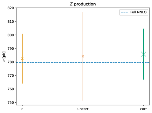
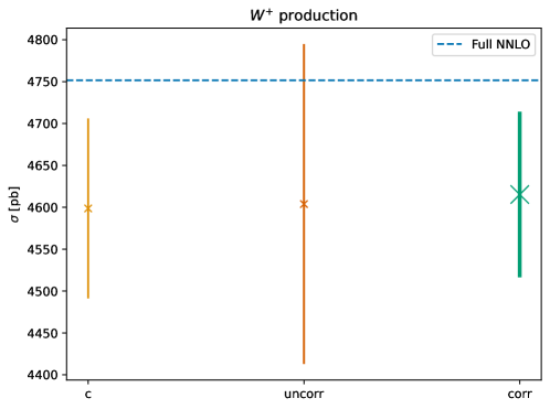
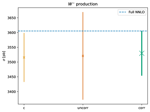
Figure 6.4: The same as Fig. 6.1 but for $Z$ (top), $W^{+}$ (middle) and $W^{-}$ (bottom) production at $\sqrt{s}=$13 TeV.

It is very interesting to observe how in this case the correlation between the scale variation in the PDF set and the scale variation in the partonic cross section decreases the total theoretical uncertainty by about a factor of 2, while bringing the result closer to the next perturbative order. This happens both for neutral and charged current Drell-Yan. In this case not including the correlation between the scale variation in the PDF set and the scale variation in the partonic cross section grossly overestimates the theoretical uncertainty of a precision observable. This is a very interesting result as the positive correlation between the scale variation in the PDFs and the scale variation in the computation of the partonic cross section makes the theoretical uncertainty smaller than in the case in which the scale uncertainty in PDFs is completely neglected.

7 Delivery

In this section we present the deliverables of this work. They consist of the MCscales PDF, which is delivered as a LHAPDF grid with enhanced metadata containing information on scale variations, as well as a set of tools to operate on it. The main deliverable of this work is PDF set obtained as described in Sect. 3, dubbed

mcscales_v1 .

It can be downloaded from the following URL:

https://data.nnpdf.science/pdfs/mcscales_v1.tar.gz .

This PDF set is based on the NNPDF 3.1 Ball:2017nwa global analysis with the same minor changes in dataset selection made in Ref. AbdulKhalek:2019ihb . The PDF set contains 823 replicas, which have been fitted with a different choice of factorisation and renormalisation scales for the input data. This allows computing predictions with matched scale variations, as discussed in Sec. 4.1, such as those used in the phenomenology studies in Sec. 6. These computations could be implemented directly on codes, with the help of the metadata information stored in the LHAPDF grids discussed next, or executed manually on any code that allows choosing PDFs and scales, with the help of a script to split the grids, which we also provide and describe briefly below.

The metadata of the LHAPDF grid of the mcscales_v1 set has been enhanced with the following keys in the global .info file affecting the full PDF set:

mcscales_processes

A list of strings containing the processes for which separate renormalisation scales are considered, as discussed in Sec. 2.1. Its current value is [DIS CC, DIS NC, DY, JETS, TOP].

mcscales_scale_multipliers

A list of numbers with the possible scale multiplier choices, Eq. 2.1. Its current value is [0.5, 1, 2].

The metadata header for each of replica grids (that is, all the members of the LHAPDF set except the data member 0, which corresponds to the central value) has been enhanced with the following keys:

mcscales_ren_multiplier_<PROCESS>

: One key for each of the values of mcscales_processes (i.e. mcscales_ren_multiplier_DIS CC, mcscales_ren_multiplier_DIS NC,mcscales_ren_multiplier_DY, mcscales_ren_multiplier_JETS and mcscales_ren_multiplier_TOP) with the value of the renormalisation scale multiplier for a given process and the current replica. The possible values are one of the entries in mcscales_scale_multipliers.

mcscales_fac_multiplier

The factorisation scale multiplier for the current replica. The possible values are one of the entries in mcscales_scale_multipliers.

This metadata, accessible with the LHAPDF library, should allow for incorporating support for the matched scale convolution described in Sect. 4.1: Users can split the replicas by scale multipliers as appropriate for the computation and match the scale variation for the hard cross section with each group, in order to implement either Eq. 4.3 or Eq. 4.4.

In addition, we provide a set of tools to manipulate MCscales PDFs. These are available from

https://github.com/Zaharid/mcscales_tools/  .

The repository contains two scripts, along with usage instructions. Here we provide a brief overview.

The first one mcscales-partition-pdf is used partition one MCscales PDF into several PDF sets with identical renormalisation or factorisation scale choices across all replicas in a given set. These can be either three sets, split by factorization scale variation, and with arbitrary renormalisation scales, or nine sets, split by factorisation or renormalisation scale variations for a given process, which is given as input. This allows implementing matched convolution computations with existing tools. The computation of a given cross section is repeated for all PDF sets in the split, taking care to compute the hard cross section with the matched scale variation for each set. Eqs. 4.3 and 4.4 can then be implemented with a nine way (factorization and renormalisation scale for a given process) and a tree way (factorisation scale) split respectively. This strategy was used to obtain the results in Sec. 6 with a variety of existing codes.

The second script, mcscales-resample-pdf, allows to experiment with simple variatons of the prior scale choices. It generates a new MCscales PDF set by vetoing particular scale combinations from an original MCscales PDF set. We note that owing to the particularly simple form of the choice of postfit likelihood in Eq. 2.7, this is identical to modifying the prior distribution of scales (as long as central scale choices are kept). The script allows reproducing the PDF sets shown in Sect. 3.4, with different variations on the prior. Users are encouraged to modify the source code of this script in order to investigate more general scale priors, such as those discussed in Appendix A.

8 Conclusion

In this work we have presented a PDF determination that includes scale uncertainties by expanding the Monte Carlo sampling method for propagating experimental uncertainties to PDFs to the space of factorisation and renormalisation scales. In this approach, dubbed MCscales, the scales are viewed as free parameters of the fixed-order theory that should be chosen jointly so as to produce theory predictions that are compatible with experimental data included the PDF fit.

This method has several key benefits. First of all, the information provided in LHAPDF sets is extended to include the scales used to produce each PDF replica. As a result, external users are able to modify the PDF set based on their preferences. Second, this added scale information can be utilised to correlate scale variations in partonic cross sections with those in the MCscales PDF set that we provide.

Having explicitly set out the assumptions used to construct a prior distribution of scales in the MCscales approach, we have demonstrated that both experimental data and theoretical considerations can be used to constrain the prior.

Our procedure provides a way to benchmark the suitability of different scales variations across all the data in PDF fits, allowing to educe a quantitative underpinning from this traditional procedure. We observed that the customary variation range of a factor of two around a central scale performs differently when applied to factorisation and renormalisation scales. For factorisation scales, a variation of a factor 2 adequately covers the set of values that are likely to yield a satisfactory fit to the data. This conclusion however relies on the fitting of the PDF replicas and post selection procedure described in Sect. 2. Indeed, performing such scale variations without our procedure implies PDFs that are not in agreement with the experimental data, which is the only source of information on precise constraints of PDFs, and therefore, unphysical predictions. We observed that this is not the case for renormalisation scale variations of a factor of two, which instead exhibit a rather uniform fit quality for the three choices. This suggests that the theoretical uncertainty on the renormalisation scale might be underestimated, at least at NLO and with appropriate matching between PDF and hard cross section. We leave for future work to study scale variation ranges in more detail. Furthermore we observed that the behaviour of scale choices was highly variable across different processes, suggesting that a method that treats each process in the same way (as in the theory covariance matrix approach) may be undesirable. At the PDF level, the MCscales approach appears to lead to rather larger PDF uncertainties. However, since in the MCscales approach each PDF replica uses theoretical predictions with matched scale combinations, comparisons at the PDF level are misleading. Indeed we noticed that convolutions with matched scales can both increase and decrease the uncertainty on cross sections as compared to the uncertainties on PDF themselves.

We exploited the possibility of modifying the prior distribution of scales by simply choosing to omit certain scale combinations, producing MCscales variants based on priors that include only the 7-points in the renormalisation and factorisation scale space that are included in the widely adopted 7-points envelope. This led to us observing that excluding the scale combinations with ratios of four or one-quarter (i.e. those excluded in 7-point) drives a significant reduction in the MCscales PDF uncertainties.

Finally, we moved to phenomenology by, firstly, setting out recipes for making predictions with MCscales PDF sets, and then applying these to processes relevant to the LHC. We demonstrated that it is possible to include correlations between scale variations in the hard cross section and those in the PDF, whether or not the process in question is included in the PDF fit. As with the theory covariance matrix approach, the inclusion of scale uncertainties with MCscales leads generally to more accurate predictions. The increase in uncertainty induced by their inclusion (if indeed there is an increase) is typically slightly larger when using MCscales than the theory covariance matrix, though they remain mild, at around the 1% level. Many developments are possible on the common assumptions of the two methods, including a more refined factorisation scale variations or more nuanced process categorisations. Such extensions are possible avenues for future research. That said, the most pressing phenomenological development will be the extension of both methodologies to the determination of MHOUs in a state-of-the-art NNLO PDF set. Indeed, the inclusion of different sources of theoretical uncertainties at NNLO is expected to lead to the most precise and accurate PDF sets currently attainable. The MCscales methodology could be naturally extended to handle these uncertainties.

Appendix A The $\alpha\beta\gamma$ model

As it was mentioned in the paper, the MCscales approach allows the users to select a specific prior probability in the space of factorisation and renormalisation scales. Any user could apply any symmetric or asymmetric choice of scales depending on their theoretical preference. In this Appendix we outline a particular theoretical model, dubbed the $\alpha\beta\gamma$ model, that a user could choose to construct a more convolved prior probability than the uniform priors presented in the main paper and tune it according to the user’s theoretical assumptions on the correlation between processes. The model can be seen as a generalisation for the prior choices considered in Sect. 3, which can be recovered for certain values of the parameters. In the second part of the Appendix, we determine the value of the $\alpha\beta\gamma$ parameters that the data included in the fit tend to prefer.

A.1 Prior assumptions

We construct the model for the prior probability by imposing a set of theoretically-motivated symmetries. As we will show below, we can characterise the prior probability for each theory hypothesis in terms of a set of total probabilities for each scale, defined as the sum of the probabilities of all the hypotheses where a particular scale variation $k_{i}$ has a given value, $x$,

$$P(k_{i}=x)=\sum_{\{\omega\in\Omega|\xi_{i}=x\}}P(\omega)\ ,$$ (A.1)

and set of conditional probabilities

$$P(k_{i}=x|k_{j}=y)=\frac{1}{P(k_{j}=y)}\sum_{\{\omega\in\Omega|\xi_{i}=x,\xi_{j}=y\}}P(\omega)\ .$$ (A.2)

Symmetry between renormalisation and factorisation scales

When considering only one process, we assume that the probability is invariant under the exchange of the factorisation and the renormalisation scales. Thus, when sampling independently, we have,

$$P(k_{f}=\xi)=P(k_{r}=\xi)\ ,$$ (A.3)

with the conditional probabilities also being symmetric,

$$P(k_{f}=\xi_{x}|k_{r}=\xi_{y})=P(k_{r}=\xi_{x}|k_{f}=\xi_{y})\ .$$ (A.4)

Symmetry between upper and lower variations

We assume that the probabilities are unchanged if we flip all of the upper and lower scale variations. That is, given

$$\text{flip}(\xi)=\begin{cases}2&\xi=\frac{1}{2}\\ 1&\xi=1\\ \frac{1}{2}&\xi=2\end{cases}\ ,$$ (A.5)

we assume

$$P\left(\xi_{f},\xi_{1},\ldots,\xi_{N_{\text{p}}}\right)=P\left(\text{flip}(\xi_{f}),\text{flip}(\xi_{1}),\ldots,\text{flip}(\xi_{N_{\text{p}}})\right)\ .$$ (A.6)

Conditional independence between renormalisation scales

We assume that the probabilities of sampling different renormalisation scales are conditionally independent given the factorisation scale. That is, for $i\neq j$,

$$P(k_{r_{i}}=\xi_{i}|k_{f}=\xi_{f},k_{r_{j}}=\xi_{j})=P(k_{r_{i}}=\xi_{i}|k_{f}=\xi_{f})\ .$$ (A.7)

Note that this does not imply $P(k_{r_{i}}=\xi_{i}|k_{r_{j}}=\xi_{j})=P(k_{r_{i}}=\xi_{i})$ since knowledge of $k_{r_{j}}$ provides knowledge on $k_{f}$ and thus renormalisation scale variations are in principle correlated with each other.

Symmetry between renormalisation scales

We assume that the probabilities are unchanged under permutations of the values of the renormalisation scales. In particular, this implies

$$P(k_{r_{i}}=\xi)=P(k_{r_{j}}=\xi)$$ (A.8)

and

$$P(k_{r_{i}}=\xi|k_{f}=\xi_{f})=P(k_{r_{j}}=\xi|k_{f}=\xi_{f})$$ (A.9)

for all $i,j\in 1,\ldots,N_{\text{p}}$.

Because we assume that renormalisation scale variations are independent (Eq. (A.7)), we can give the probability of any set of scale variations in terms of the total probability of sampling a given value of the factorisation scale and conditional probabilities for sampling a renormalisation scale given the factorisation scale:

$$P(k_{f}=\xi_{f},\ldots,k_{r_{N_{\text{p}}}}=\xi_{N_{\text{p}}})=P(k_{f}=\xi_{f})\prod_{i=1}^{N_{\text{p}}}P(k_{r_{i}}=\xi_{i}|k_{f}=\xi_{f})\ .$$ (A.10)

Let us now count how many parameters we must specify to define all of the probabilities. To begin, we have to specify three values for $P(k_{f})$. Further, because we assume that the model acts the same for all renormalisation scales (Eq. (A.8)), we have to specify nine values for the conditional probabilities, one for each combination of renormalisation and factorisation scale variation. These 12 total values are not independent, as they are constrained by one normalisation relation for the total factorisation scale variation probabilities,

$$\sum_{\xi\in\Xi}P(k_{f}=\xi)=1\,,$$ (A.11)

and three relations for the conditional probabilities, one for each possible value of $\xi_{f}$,

$$\sum_{\xi\in\Xi}P(k_{r}=\xi|k_{f}=\xi_{f})=1\qquad\forall\,\xi_{f}\in\Xi\,.$$ (A.12)

We have four additional constraints from the symmetry of upper and lower variations (Eq. (A.6)),

$$P\left(k_{f}=\frac{1}{2}\right)= P(k_{f}=2)$$

$$P\left(k_{r}=\frac{1}{2}|k_{f}=1\right)= P(k_{r}=2|k_{f}=1)$$

$$P\left(k_{r}=1|k_{f}=\frac{1}{2}\right)= P(k_{r}=1|k_{f}=2)$$

$$P\left(k_{r}=\frac{1}{2}|k_{f}=2\right)= P\left(k_{r}=2|k_{f}=\frac{1}{2}\right)\,.$$

Finally, the symmetry between factorisation and renormalisation scales (Eq. (A.4)) adds another constrain,

$$P(k_{r}=1|k_{f}=2)=\frac{P(k_{f}=2|k_{r}=1)P(k_{r}=1)}{P(k_{f}=2)}=\frac{P(k_{r}=2|k_{f}=1)P(k_{f}=1)}{P(k_{f}=2)}\ ,$$ (A.13)

where in the first equality we have used the law of conditional probabilities (Bayes’ theorem).

It follows that with our assumptions, the sampling model is completely specified with three free parameters, which we call $\alpha$, $\beta$ and $\gamma$. We can choose them to be probability ratios; we define $\alpha$ as the probability of sampling a central factorisation scale, over the probability to sample a non-central scale,

$$\alpha\equiv\frac{P(k_{f}=1)}{P(k_{f}=2)}=\frac{P(k_{f}=1)}{P(k_{f}=\frac{1}{2})}\,,$$ (A.14)

$\beta$ to be the ratio of probabilities for central and non-central variations given that a central factorisation scale is chosen,

$$\beta\equiv\frac{P(k_{r}=1|k_{f}=1)}{P(k_{r}=2|k_{f}=1)}=\frac{P(k_{r}=1|k_{f}=1)}{P(k_{r}=\frac{1}{2}|k_{f}=1)}\,,$$ (A.15)

and $\gamma$ as the probability of sampling the same upper or lower renormalisation scale as the factorisation scale, over the probability of sampling the opposite renormalisation scale given the same factorisation scale as in the numerator,

$$\gamma\equiv\frac{P(k_{r}=2|k_{f}=2)}{P(k_{r}=\frac{1}{2}|k_{f}=2)}=\frac{P(k_{r}=\frac{1}{2}|k_{f}=\frac{1}{2})}{P(k_{r}=2|k_{f}=\frac{1}{2})}\,.$$ (A.16)

In terms of the parameters, the probabilities are

$$P(k_{f}=1) =\frac{\alpha}{2+\alpha}$$

$$P\left(k_{f}=\frac{1}{2}\right)=P(k_{f}=2) =\frac{1}{2+\alpha}$$

$$P(k_{r}=1|k_{f}=1) =\frac{\beta}{2+\beta}$$

$$P\left(k_{r}=\frac{1}{2}|k_{f}=1\right)=P(k_{r}=2|k_{f}=1) =\frac{1}{2+\beta}$$ (A.17)

$$P\left(k_{r}=1|k_{f}=\frac{1}{2}\right)=P(k_{r}=1|k_{f}=2) =\frac{\alpha}{2+\beta}$$

$$P\left(k_{r}=\frac{1}{2}|k_{f}=\frac{1}{2}\right)=P(k_{r}=2|k_{f}=2) =\frac{c(\beta+2-\alpha)}{(2+\beta)(1+\gamma)}$$

$$P\left(k_{r}=\frac{1}{2}|k_{f}=2\right)=P\left(k_{r}=2|k_{f}=\frac{1}{2}\right) =\frac{(\beta+2-\alpha)}{(2+\beta)(1+\gamma)}$$

Note that these parameters have a clear physical interpretation. For example, a model where factorisation and renormalisation variations are completely independent corresponds to $\alpha=\beta$ and $\gamma=1$, a model where they are completely correlated corresponds to $\beta\to\infty$ and $\gamma\to\infty$, while $\alpha=\beta=1,\gamma\to\infty$ corresponds to the prescription where the extreme asymmetric variations are discarded while the rest have the same probability (sometimes referred to as the 7-point prescription).

A.2 Data-driven determination of the $\alpha\beta\gamma$ coefficients

Thus far our analysis of the replica distributions over scale choices has been largely qualitative. To make it more quantitative we now define some effective values of $\alpha$, $\beta$ and $\gamma$, which can be computed from the aforementioned distributions to give an indication of the particular $\alpha\beta\gamma$ model that the resulting PDF set corresponds to. Here we define effective model parameters by modifying Eqs (A.14), (A.15) and (A.16), where the modifications take into account the fact that the symmetries of the model are broken after postfit vetoes are imposed.

Beginning with $\alpha$, we see that in Eq. (A.14) it is defined in two ways, which are of course equal due to the model assumptions of the $\alpha\beta\gamma$ model, where $P(k_{f}=\frac{1}{2})=P(k_{f}=2)$. However, after the postfit vetoes have been applied this equality is unlikely to hold. This breaking of the model symmetries can be seen for example in Fig. 3.3. Therefore, if we evaluate $\frac{P(k_{f}=1)}{P(k_{f}=\frac{1}{2})}$ in the hope of defining an effective value for $a$ and then compare it to $\frac{P(k_{f}=1)}{P(k_{f}=2)}$, we will get different answers. In order to give a rough estimate of the effective value of $\alpha$, we therefore symmetrise the distribution over $k_{f}$ and define

$$\alpha_{\text{eff}}=\frac{P(k_{f}=1)}{(P(k_{f}=\frac{1}{2})+P(k_{f}=2))/2}\,.$$ (A.18)

Similarly,

$$\beta_{\text{eff}}=\frac{1}{N_{\text{p}}}\sum_{p=1}^{N_{\text{p}}}\frac{P(k_{r_{p}}=1|k_{f}=1)}{(P(k_{r_{p}}=\frac{1}{2}|k_{f}=1)+P(k_{r_{p}}=2|k_{f}=1))/2}\,,$$ (A.19)

where we average over processes because the summand will in general be different for each process. This is because the postfit vetoes act differently on different processes.

Finally,

$$\gamma_{\text{eff}} =\frac{1}{N_{\text{p}}}\sum_{p=1}^{N_{\text{p}}}\frac{(P(k_{r_{p}}=\frac{1}{2}|k_{f}=\frac{1}{2})+P(k_{r_{p}}=2|{k_{f}}=2))/2}{(P({k_{r_{p}}}=\frac{1}{2}|k_{f}=2)+P(k_{r_{p}}=2|k_{f}=\frac{1}{2}))/2}$$ (A.20)

$$=\frac{1}{N_{\text{p}}}\sum_{p=1}^{N_{\text{p}}}\frac{P(k_{r_{p}}=\frac{1}{2}|k_{f}=\frac{1}{2})+P(k_{r_{p}}=2|k_{f}=2)}{P(k_{r_{p}}=\frac{1}{2}|k_{f}=2)+P(k_{r_{p}}=2|k_{f}=\frac{1}{2})}\,.$$ (A.21)

In Table A.1 we show these effective model parameters for the two MCscales PDF sets that we are studying in this section. Note that in the case that all of the replicas do satisfy the $\alpha\beta\gamma$ model symmetries, which is the case for the MCscales replicas without postfit applied, the effective model parameters coincide with the model parameters that were chosen as input, namely $a=b=c=1$, as we would expect.

Parameter	MCscales without postfit	MCscales with postfit
$\alpha_{\text{eff}}$	1.0	3.2
$\beta_{\text{eff}}$	1.0	1.1
$\gamma_{\text{eff}}$	1.0	1.4

Table A.1: Estimates of the effective model parameters before and after applying postfit vetoes, where for $\beta_{\text{eff}}$ and $\gamma_{\text{eff}}$ the values are averaged over processes.

These effective parameters for the MCscales PDF set with postfit indicate the $\alpha\beta\gamma$ model that best fits the experimental data. We see that a value of $\alpha_{\text{eff}}\sim 3$ is preferred, which indicates that $P(k_{f}=1)\approx 3P(k_{f}=\frac{1}{2})\approx 3P(k_{f}=2)$ and therefore the degree to which the central factorisation scale fits the data better than the non-central factorisation scales. Next we see that $\beta_{\text{eff}}\sim 1$, which tells us that given a replica with $k_{f}=1$, the fit quality is roughly independent of the processes renormalisation scale, since $P(k_{r}=1|k_{f}=1)\approx P(k_{r}=1|k_{f}=\frac{1}{2})\approx P(k_{r}=1|k_{f}=2)$ is implied. Finally, we see that $\gamma_{\text{eff}}=1.4$, which tells us that for the non-central factorisation scales, there is a mild asymmetry in the renormalisation scales, with a slight preference for the same renormalisation scale multipliers as the factorisation scale multiplier.

The values of $\beta_{\text{eff}}$ and $c_{\text{eff}}$ discussed above have been averaged over processes. We can also compute these effective parameters per process, which we show in Table A.2. For $\beta_{\text{eff}}$ we see a small variance of the values for the MCscales set with postfit, with the numbers exhibiting small fluctuations around the mean value of 1.1. For $\gamma_{\text{eff}}$ the fluctuations are more pronounced, with values of around one being preferred for the DY, jet and top data, and significantly higher values being preferred for the DIS data. This suggests that the DY, jet and top data are more stable upon variations of the renormalisation scale from a given non-central factorisation scale, and indeed the goodness of fit is almost independent of these variations. This is in fact true for the jet and top data, but misleading for the DY data, where we see from Fig. 3.3 that the distribution is in fact highly skewed, which is something not captured by $\gamma_{\text{eff}}$. The fact that the DIS data correspond to higher values of $\gamma_{\text{eff}}$, particularly for the DIS NC data, matches the observations drawn from Fig. 3.3. This is true especially for the DIS NC data, for which we recall that the $(k_{f},k_{r})=(2,\frac{1}{2})$ bin is entirely unfilled after postfit has been applied.

Parameter	Process	MCscales without postfit	MCscales with postfit
$\beta_{\text{eff}}$	DIS CC	1.0	1.2
	DIS NC	0.9	1.0
	DY	1.0	1.3
	Jet	0.9	0.9
	Top	1.0	1.2
$\gamma_{\text{eff}}$	DIS CC	1.0	1.6
	DIS NC	1.1	2.3
	DY	1.0	1.1
	Jet	0.9	1.0
	Top	1.0	0.9

Table A.2: Estimates of the effective values of $\beta$ and $\gamma$ per process. Note that $\alpha$ is not shown because it does not differ between processes. Note also that the results for the MCscales set without postfit should each be equal to one in the limit of infinite statistics, and that the reason they are not is due to insufficient PDF replicas.

The variability of these parameters across processes suggests that using a model that treats these five processes on the same footing is perhaps ill advised. For example, it is perhaps not preferable to include results for $(k_{f},k_{r})=(2,\frac{1}{2})$ for DIS NC on the same footing as all other combinations, when this particular combination leads to such poor agreement with the data. Indeed, the $\alpha\beta\gamma$ model withut any post selection does exactly this, as do the current implementations of the theoretical covariance matrix. However, importantly, after postfit has been applied, this is no longer the case for the $\alpha\beta\gamma$ model. We consider this to be an advantage of the MCscales PDF set with postfit applied over other PDF sets with scale variations taken into account. As can be seen from Fig. 3.3, despite the fact that the processes are initially treated equally, they very much are not after postfit has been applied.

References

- (1) NNPDF Collaboration, R. D. Ball et al., Parton distributions from high-precision collider data, Eur. Phys. J. C77 (2017), no. 10 663, [arXiv:1706.00428].
- (2) S. Bailey, T. Cridge, L. A. Harland-Lang, A. D. Martin, and R. S. Thorne, Parton distributions from LHC, HERA, Tevatron and fixed target data: MSHT20 PDFs, arXiv:2012.04684.
- (3) T.-J. Hou et al., New CTEQ global analysis of quantum chromodynamics with high-precision data from the LHC, Phys. Rev. D 103 (2021), no. 1 014013, [arXiv:1912.10053].
- (4) NNPDF Collaboration, R. D. Ball et al., The path to proton structure at 1% accuracy, Eur. Phys. J. C 82 (2022), no. 5 428, [arXiv:2109.02653].
- (5) R. D. Ball et al., The PDF4LHC21 combination of global PDF fits for the LHC Run III, arXiv:2203.05506.
- (6) S. Amoroso et al., Snowmass 2021 whitepaper: Proton structure at the precision frontier, arXiv:2203.13923.
- (7) R. Abdul Khalek, S. Bailey, J. Gao, L. Harland-Lang, and J. Rojo, Towards Ultimate Parton Distributions at the High-Luminosity LHC, Eur. Phys. J. C78 (2018), no. 11 962, [arXiv:1810.03639].
- (8) NNPDF Collaboration, R. D. Ball et al., Parton distributions for the LHC Run II, JHEP 04 (2015) 040, [arXiv:1410.8849].
- (9) L. Del Debbio, T. Giani, and M. Wilson, Bayesian approach to inverse problems: an application to NNPDF closure testing, Eur. Phys. J. C 82 (2022), no. 4 330, [arXiv:2111.05787].
- (10) J. Cruz-Martinez, S. Forte, and E. R. Nocera, Future tests of parton distributions, Acta Phys. Polon. B 52 (2021) 243, [arXiv:2103.08606].
- (11) T. Carli, D. Clements, A. Cooper-Sarkar, C. Gwenlan, G. P. Salam, F. Siegert, P. Starovoitov, and M. Sutton, A posteriori inclusion of parton density functions in nlo qcd final-state calculations at hadron colliders: the applgrid project, The European Physical Journal C 66 (Apr, 2010) 503–524.
- (12) V. Bertone, S. Carrazza, and N. P. Hartland, APFELgrid: a high performance tool for parton density determinations, Comput. Phys. Commun. 212 (2017) 205–209, [arXiv:1605.02070].
- (13) T. Kluge, K. Rabbertz, and M. Wobisch, FastNLO: Fast pQCD calculations for PDF fits, in 14th International Workshop on Deep Inelastic Scattering, 9, 2006. hep-ph/0609285.
- (14) R. Frederix, S. Frixione, V. Hirschi, D. Pagani, H. S. Shao, and M. Zaro, The automation of next-to-leading order electroweak calculations, JHEP 07 (2018) 185, [arXiv:1804.10017]. [Erratum: JHEP 11, 085 (2021)].
- (15) S. Carrazza, E. R. Nocera, C. Schwan, and M. Zaro, PineAPPL: combining EW and QCD corrections for fast evaluation of LHC processes, JHEP 12 (2020) 108, [arXiv:2008.12789].
- (16) J. McGowan, T. Cridge, L. A. Harland-Lang, and R. S. Thorne, Approximate N3LO Parton Distribution Functions with Theoretical Uncertainties: MSHT20aN3LO PDFs, arXiv:2207.04739.
- (17) M. Cacciari and N. Houdeau, Meaningful characterisation of perturbative theoretical uncertainties, JHEP 09 (2011) 039, [arXiv:1105.5152].
- (18) A. David and G. Passarino, How well can we guess theoretical uncertainties?, Phys. Lett. B 726 (2013) 266–272, [arXiv:1307.1843].
- (19) M. Bonvini, Probabilistic definition of the perturbative theoretical uncertainty from missing higher orders, Eur. Phys. J. C 80 (2020), no. 10 989, [arXiv:2006.16293].
- (20) C. Duhr, A. Huss, A. Mazeliauskas, and R. Szafron, An analysis of Bayesian estimates for missing higher orders in perturbative calculations, arXiv:2106.04585.
- (21) NNPDF Collaboration, R. Abdul Khalek et al., A first determination of parton distributions with theoretical uncertainties, Eur. Phys. J. C (2019) 79:838, [arXiv:1905.04311].
- (22) NNPDF Collaboration, R. Abdul Khalek et al., Parton Distributions with Theory Uncertainties: General Formalism and First Phenomenological Studies, Eur. Phys. J. C 79 (2019), no. 11 931, [arXiv:1906.10698].
- (23) R. D. Ball, E. R. Nocera, and R. L. Pearson, Deuteron Uncertainties in the Determination of Proton PDFs, Eur. Phys. J. C 81 (2021), no. 1 37, [arXiv:2011.00009].
- (24) R. Pearson, R. Ball, and E. R. Nocera, Uncertainties due to Nuclear Data in Proton PDF Fits, PoS DIS2019 (2019) 027.
- (25) L. A. Harland-Lang and R. S. Thorne, On the Consistent Use of Scale Variations in PDF Fits and Predictions, Eur. Phys. J. C79 (2019), no. 3 225, [arXiv:1811.08434].
- (26) R. D. Ball and R. L. Pearson, Decorrelation of Theoretical Uncertainties in PDF Fits and Theoretical Uncertainties in Predictions, arXiv:2105.05114.
- (27) A. Buckley, J. Ferrando, S. Lloyd, K. Nordström, B. Page, M. Rüfenacht, M. Schönherr, and G. Watt, LHAPDF6: parton density access in the LHC precision era, Eur. Phys. J. C 75 (2015) 132, [arXiv:1412.7420].
- (28) S. Iranipour and M. Ubiali, A new generation of simultaneous fits to LHC data using deep learning, JHEP 05 (2022) 032, [arXiv:2201.07240].
- (29) M. McCullough, J. Moore, and M. Ubiali, The dark side of the proton, arXiv:2203.12628.
- (30) A. Greljo, S. Iranipour, Z. Kassabov, M. Madigan, J. Moore, J. Rojo, M. Ubiali, and C. Voisey, Parton distributions in the SMEFT from high-energy Drell-Yan tails, JHEP 07 (2021) 122, [arXiv:2104.02723].
- (31) W. T. Giele, S. A. Keller, and D. A. Kosower, Parton Distribution Function Uncertainties, hep-ph/0104052.
- (32) NNPDF Collaboration, R. D. Ball, L. Del Debbio, S. Forte, A. Guffanti, J. I. Latorre, A. Piccione, J. Rojo, and M. Ubiali, A Determination of parton distributions with faithful uncertainty estimation, Nucl. Phys. B 809 (2009) 1–63, [arXiv:0808.1231]. [Erratum: Nucl.Phys.B 816, 293 (2009)].
- (33) R. D. Ball, L. Del Debbio, S. Forte, A. Guffanti, J. I. Latorre, J. Rojo, and M. Ubiali, A first unbiased global NLO determination of parton distributions and their uncertainties, Nucl. Phys. B 838 (2010) 136–206, [arXiv:1002.4407].
- (34) R. D. Ball et al., Parton distributions with LHC data, Nucl. Phys. B 867 (2013) 244–289, [arXiv:1207.1303].
- (35) NNPDF Collaboration, L. Del Debbio, R. D. Ball, S. Forte, A. Guffanti, J. I. Latorre, A. Piccione, J. Rojo, and M. Ubiali, Monte Carlo methods for robust error estimates for PDFs, in 44th Rencontres de Moriond on QCD and High Energy Interactions, 3, 2009.
- (36) NNPDF Collaboration, R. D. Ball, V. Bertone, F. Cerutti, L. Del Debbio, S. Forte, A. Guffanti, J. I. Latorre, J. Rojo, and M. Ubiali, Parton Distributions: Determining Probabilities in a Space of Functions, in PHYSTAT 2011, 10, 2011. arXiv:1110.1863.
- (37) LHC Higgs Cross Section Working Group Collaboration, D. de Florian et al., Handbook of LHC Higgs Cross Sections: 4. Deciphering the Nature of the Higgs Sector, arXiv:1610.07922.
- (38) NNPDF Collaboration, R. D. Ball, L. Del Debbio, S. Forte, A. Guffanti, J. I. Latorre, J. Rojo, and M. Ubiali, Fitting Parton Distribution Data with Multiplicative Normalization Uncertainties, JHEP 05 (2010) 075, [arXiv:0912.2276].
- (39) R. D. Ball et al., Parton Distribution Benchmarking with LHC Data, JHEP 04 (2013) 125, [arXiv:1211.5142].
- (40) H1, ZEUS Collaboration, H. Abramowicz et al., Combination and QCD Analysis of Charm Production Cross Section Measurements in Deep-Inelastic ep Scattering at HERA, Eur. Phys. J. C73 (2013), no. 2 2311, [arXiv:1211.1182].
- (41) H1, ZEUS Collaboration, H. Abramowicz et al., Combination and QCD analysis of charm and beauty production cross-section measurements in deep inelastic scattering at HERA, Eur. Phys. J. C 78 (2018), no. 6 473, [arXiv:1804.01019].
- (42) S. Forte and Z. Kassabov, Why cannot be determined from hadronic processes without simultaneously determining the parton distributions, Eur. Phys. J. C 80 (2020), no. 3 182, [arXiv:2001.04986].
- (43) A. Barontini, A. Candido, J. M. Cruz-Martinez, F. Hekhorn, and C. Schwan, Pineline: Industrialization of High-Energy Theory Predictions, arXiv:2302.12124.
- (44) C. Anastasiou, C. Duhr, F. Dulat, F. Herzog, and B. Mistlberger, Higgs Boson Gluon-Fusion Production in QCD at Three Loops, Phys. Rev. Lett. 114 (2015) 212001, [arXiv:1503.06056].
- (45) C. Anastasiou, C. Duhr, F. Dulat, E. Furlan, T. Gehrmann, F. Herzog, A. Lazopoulos, and B. Mistlberger, High precision determination of the gluon fusion Higgs boson cross-section at the LHC, JHEP 05 (2016) 058, [arXiv:1602.00695].
- (46) B. Mistlberger, Higgs boson production at hadron colliders at N3LO in QCD, JHEP 05 (2018) 028, [arXiv:1802.00833].
- (47) F. A. Dreyer and A. Karlberg, Vector-Boson Fusion Higgs Production at Three Loops in QCD, Phys. Rev. Lett. 117 (2016), no. 7 072001, [arXiv:1606.00840].
- (48) M. Bonvini, R. D. Ball, S. Forte, S. Marzani, and G. Ridolfi, Updated Higgs cross section at approximate N3LO, J. Phys. G 41 (2014) 095002, [arXiv:1404.3204].
- (49) M. Bonvini, S. Marzani, C. Muselli, and L. Rottoli, On the Higgs cross section at N3LO+N3LL and its uncertainty, JHEP 08 (2016) 105, [arXiv:1603.08000].
- (50) M. Cacciari, F. A. Dreyer, A. Karlberg, G. P. Salam, and G. Zanderighi, Fully Differential Vector-Boson-Fusion Higgs Production at Next-to-Next-to-Leading Order, Phys. Rev. Lett. 115 (2015), no. 8 082002, [arXiv:1506.02660]. [Erratum: Phys.Rev.Lett. 120, 139901 (2018)].
- (51) M. Czakon and A. Mitov, Top++: A Program for the Calculation of the Top-Pair Cross-Section at Hadron Colliders, Comput. Phys. Commun. 185 (2014) 2930, [arXiv:1112.5675].
- (52) Y. Li and F. Petriello, Combining QCD and electroweak corrections to dilepton production in FEWZ, Phys. Rev. D 86 (2012) 094034, [arXiv:1208.5967].
- (53) R. Gavin, Y. Li, F. Petriello, and S. Quackenbush, W Physics at the LHC with FEWZ 2.1, Comput. Phys. Commun. 184 (2013) 208–214, [arXiv:1201.5896].
- (54) R. Gavin, Y. Li, F. Petriello, and S. Quackenbush, FEWZ 2.0: A code for hadronic Z production at next-to-next-to-leading order, Comput. Phys. Commun. 182 (2011) 2388–2403, [arXiv:1011.3540].