PLSS: A Projected Linear Systems Solver

Abstract

We propose iterative projection method s for solving square or rectangular consistent linear systems $\mathbf{A}\mathbf{x}=\mathbf{b}$. Existing projection methods use sketching matrices (possibly randomized) to generate a sequence of small projected subproblems, but even the smaller systems can be costly. We develop a process that appends one column to the sketching matrix each iteration and converges in a finite number of iterations whether the sketch is random or deterministic. In general, our process generates orthogonal updates to the approximate solution $\mathbf{x}_{k}$. By choosing the sketch to be the set of all previous residuals, we obtain a simple recursive update and convergence in at most $\text{rank}(\mathbf{A})$ iterations (in exact arithmetic). By choosing a sequence of identity columns for the sketch, we develop a generalization of the Kaczmarz method. In experiments on large sparse systems, our method (PLSS) with residual sketches is competitive with LSQR and LSMR, and with residual and identity sketches compares favorably with state-of-the-art randomized methods.

15A06, 15B52, 65F10, 68W20, 65Y20, 90C20

1 Introduction

Consider a general linear system

(1) $$\mathbf{A}\mathbf{x}=\mathbf{b},\qquad\mathbf{b}\in\textrm{range}(\mathbf{A}),$$

where $\mathbf{A}\in\mathbb{R}^{m\times n}$, $\mathbf{x}\in\mathbb{R}^{n}$ and $\mathbf{b}\in\mathbb{R}^{m}$. For computations with large matrices, randomized methods [6, 7, 16] aim to generate inexpensive (possibly low-accuracy) estimates of $\mathbf{x}$ by solving smaller projected systems. When the elements of $\mathbf{A}$ are contaminated by errors or noise, which may be the case in data-driven problems, highly accurate solutions are not always requested. For large systems, randomized solvers are growing in popularity, although it is not uncommon to observe slow convergence for naive implementations. Reasons for the widespread interest may be the arguably intuitive approach of solving a sequence of small projected systems instead of (1), and the fact that randomization has emerged as an enabling technology in data science. This article develops a family of projection methods that solve a sequence of smaller systems and can have significant advantages in terms of computation, accuracy, and convergence.

1.1 Notation

Integer $k\geq{\color[rgb]{0,0,0}1}$ represents the iteration index, and vector $\mathbf{e}_{k}$ denotes the $k^{\text{th}}$ column of the identity matrix, with dimension depending on the context. The $k^{\textnormal{th}}$ row of $\mathbf{A}$ is $\mathbf{a}_{k}^{\top}=\mathbf{e}_{k}^{\top}\mathbf{A}$. For the $k^{\text{th}}$ solution estimate $\mathbf{x}_{k}$, the residual vector is $\mathbf{r}_{k}:=\mathbf{b}-\mathbf{A}\mathbf{x}_{k}$, with associated vector $\mathbf{y}_{k}:=\mathbf{A}^{\top}\mathbf{r}_{k}$. Lower-case Greek letters represent scalars, and the range of integers from $1$ to $k$ is written $1\!:\!k$. To prove convergence we make use of the economy SVD, $\mathbf{A}=\mathbf{U}{\boldsymbol{\Sigma}}\mathbf{V}^{\top}$.

1.2 Related work

To handle large problems, there has been a growing interest in sketching techniques. A straightforward approach is random sketching, which consists of selecting a random matrix $\mathbf{S}\in\mathbb{R}^{m\times r}$ with $r\ll m$ and solving the reduced linear system

(2) $$\mathbf{S}^{\top}\!\mathbf{A}\mathbf{x}=\mathbf{S}^{\top}\mathbf{b}.$$

By the Johnson-Lindenstrauss lemma [8], a solution to the reduced system (2) is related to a solution of (1). However, unless $\mathrm{range}(\mathbf{S})=\mathrm{range}(\mathbf{A})$, the solutions will not be the same. Since (2) involves the product $\mathbf{S}^{\top}\mathbf{A}$, previous work in [1, Cartis2021, 10] has focused on the choice of $\mathbf{S}$ to reduce the computational cost of this product. In particular, with certain sketching matrices $\mathbf{S}$, the randomized Kaczmarcz [17], randomized coordinate descent [11], and stochastic Newton [15] methods can be defined by (2). An overview of randomized iterative methods for solving linear systems is in [6, 16], which we consider to be state-of-the-art for the purpose of this article.

1.3 Motivation

Given $\mathbf{x}_{0}\in\mathbb{R}^{n}$, let estimates of the solution to (1) be defined by the iterative process

(3) $${\color[rgb]{0,0,0}\mathbf{x}_{k}=\mathbf{x}_{k-1}+{\color[rgb]{0,0,0}\mathbf{p}_{k}},\quad\quad k=1,2,\ldots,}$$

where ${\color[rgb]{0,0,0}\mathbf{p}_{k}}\in\mathbb{R}^{n}$ is called the update. It is important to compute the update efficiently. Because sketching techniques aim to generate iterates with relatively low computational complexity, we choose to solve a sequence of sketched systems. In particular, we use a sequence of full-rank matrices

(4) $$\mathbf{S}_{k}\in\mathbb{R}^{m\times{\color[rgb]{0,0,0}k}},\ k={\color[rgb]{0,0,0}1,2,}\dots,\qquad\textrm{rank}(\mathbf{S}_{k})={\color[rgb]{0,0,0}k}.$$

The matrices can be arbitrary as long as they have the specified dimensions and rank. We assume that $\mathbf{S}_{k}$ is in the range of $\mathbf{A}$, though this is not strictly necessary. We show later that the iterates $\mathbf{x}_{k}$ for solving (1) converge in a finite number of steps. We also demonstrate that a particular choice for $\mathbf{S}_{k}$ results in very efficient updates.

Part of our scheme is an additional full-rank parameter matrix $\mathbf{B}^{\top}\mathbf{B}\in\mathbb{R}^{n\times n}$ that can possibly improve the numerical behavior of the methods. (This matrix is not essential, and all results hold when $\mathbf{B}=\mathbf{I}_{n\times n}$.) Computations with $\mathbf{B}^{\top}\mathbf{B}$ are intended to be inexpensive, as they would be if it were a diagonal matrix. The sequence of systems that define each update are of the form

(5) $$\begin{bmatrix}\mathbf{B}^{\top}\mathbf{B}&\mathbf{A}^{\top}\mathbf{S}_{k}\\ \mathbf{S}_{k}^{\top}\mathbf{A}&\mathbf{0}_{k\times k}\end{bmatrix}\begin{bmatrix}{\color[rgb]{0,0,0}\mathbf{p}_{k}}\\ {\color[rgb]{0,0,0}{\boldsymbol{\lambda}}_{k}}\end{bmatrix}=\begin{bmatrix}\mathbf{A}^{\top}\\ \mathbf{S}_{k}^{\top}\end{bmatrix}(\mathbf{b}-\mathbf{A}\mathbf{x}_{k-1})$$

with ${\color[rgb]{0,0,0}{\boldsymbol{\lambda}}_{k}}\in\mathbb{R}^{k\times 1}$. Since only ${\color[rgb]{0,0,0}\mathbf{p}_{k}}$ is used to define the next iterates, we do not compute ${\boldsymbol{\lambda}}_{k}$. When $\mathbf{S}_{k}$ is in the range of $\mathbf{A}$, solving (5) is equivalent to the constrained least-squares problem

(6) $$\underset{\mathbf{p}\in\mathbb{R}^{n}}{\text{ arg min }}\quad \frac{1}{2}\|\mathbf{B}\mathbf{p}\|^{2}_{2}$$

(7) subject to $${\color[rgb]{0,0,0}\mathbf{S}^{\top}_{k}}\mathbf{A}({\color[rgb]{0,0,0}\mathbf{x}_{k-1}}+\mathbf{p})={\color[rgb]{0,0,0}\mathbf{S}^{\top}_{k}}\mathbf{b}.$$

Details of formulating problem (6)–(7) from (5) are in Appendix A.

Here we summarize that the solution ${\color[rgb]{0,0,0}{\color[rgb]{0,0,0}\mathbf{p}_{k}}}$ to (6)–(7) is defined by $\mathbf{W}:=(\mathbf{B}^{\top}\mathbf{B})^{-1}$ and

(8) $${\color[rgb]{0,0,0}{\color[rgb]{0,0,0}\mathbf{p}_{k}}}=\mathbf{W}\mathbf{A}^{\top}{\color[rgb]{0,0,0}\mathbf{S}_{k}}({\color[rgb]{0,0,0}\mathbf{S}^{\top}_{k}}\mathbf{A}\mathbf{W}\mathbf{A}^{\top}{\color[rgb]{0,0,0}\mathbf{S}_{k}})^{-1}{\color[rgb]{0,0,0}\mathbf{S}^{\top}_{k}}(\mathbf{b}-\mathbf{A}{\color[rgb]{0,0,0}\mathbf{x}_{k-1}}).$$

If $\mathbf{S}_{k}$ is not in the range of $\mathbf{A}$, the inverse in (8) is replaced by the pseudo-inverse. For ease of notation we set $\mathbf{B}^{\top}\mathbf{B}=\mathbf{I}$ in the next sections (and hence $\mathbf{W}=\mathbf{I}$). Later we lift this assumption and describe updates with nontrivial $\mathbf{W}$.

Once ${\color[rgb]{0,0,0}{\color[rgb]{0,0,0}\mathbf{p}_{k}}}$ is obtained from (8), it can define the next iterate via (3). Note that popular methods in [6, 16] use an update like (8); however, the matrix $\mathbf{S}\equiv\mathbf{S}_{k}$ is then typically randomly generated, and $\mathbf{A}^{\top}\mathbf{S}$, $\mathbf{S}^{\top}\mathbf{A}\mathbf{A}^{\top}\mathbf{S}$ and $(\mathbf{S}^{\top}\mathbf{A}\mathbf{A}^{\top}\mathbf{S})^{-1}$ are typically recomputed each iteration. Thus, a small parameter $r>0$ must be selected such that a random $\mathbf{S}\in\mathbb{R}^{m\times r}$ maintains low computational cost. Convergence is characterized by a rate $\rho\in[0,1)$ that depends on the smallest singular value of a matrix defined by $\mathbf{S}$ and $\mathbf{A}$. Convergence implicitly depends on the choice of $r$ and may result in prohibitively many iterations when the rate $\rho$ is close to unity.

1.4 Contributions

We prove that iteration (3)–(8) converges in $k_{\max}$ steps ($1\leq k_{\max}\leq\min(m,n)$) when the sketch is in the range of $\mathbf{A}$ or the system is underdetermined. Each sketch $\mathbf{S}_{k}$ can be random or deterministic, and can be augmented by one column each iteration or recomputed from scratch. We show that the finite-termination property holds for $m\geq n$ and also $m<n$. By selecting previous residuals to form each $\mathbf{S}_{k}$, we develop an iteration with orthogonal updates and residuals. This process is simple to implement and only stores and updates five vectors. By selecting columns of the identity matrix for each $\mathbf{S}_{k}$, we develop an update that generalizes the Kaczmarz method [9]. These choices are two instances in our general class of methods characterized by the choice of $\mathbf{S}_{k}$.

2 Method

Our method solves a sequence of sketched systems $\mathbf{S}_{k}^{\top}\mathbf{A}\mathbf{x}_{k}=\mathbf{S}_{k}^{\top}\mathbf{b}$ that exploit information generated at previous iterations. Suppose that one sketching column $\mathbf{s}_{k}$ is generated each iteration and stored in the matrix

(9) $$\mathbf{S}_{k}:=\begin{bmatrix}\mathbf{s}_{1}&\mathbf{s}_{2}&\dots&\mathbf{s}_{k}\end{bmatrix}\in\mathbb{R}^{m\times{\color[rgb]{0,0,0}k}}.$$

Throughout, we assume that $\mathbf{S}_{k}$ has full column rank.

2.1 Orthogonality

When constraints (7) are satisfied, each update has the property

(10) $$\mathbf{0}=\mathbf{S}_{k}^{\top}\mathbf{A}({\color[rgb]{0,0,0}\mathbf{x}_{k-1}+{\color[rgb]{0,0,0}\mathbf{p}_{k}}})-\mathbf{S}_{k}^{\top}\mathbf{b}=-\mathbf{S}_{k}^{\top}{\color[rgb]{0,0,0}\mathbf{r}_{k}}.$$

Therefore from (9), by construction, previous sketching columns are orthogonal to the next residual (and hence linearly independent): ${\color[rgb]{0,0,0}\mathbf{s}_{j}}\perp{\color[rgb]{0,0,0}\mathbf{r}_{i}}\textnormal{ for }{\color[rgb]{0,0,0}1}\leq j\leq{\color[rgb]{0,0,0}i},1\leq i\leq{\color[rgb]{0,0,0}k}$. In section 4 we show that the updates $\mathbf{p}_{k}$ are also orthogonal.

2.2 Practical computations

We develop general techniques to compute ${\color[rgb]{0,0,0}\mathbf{p}_{k}}$ (8) efficiently. First, we describe a method based on updating a QR factorization. Second, we deduce an alternative method (based on updating a triangular factorization) to avoid recomputing ${\color[rgb]{0,0,0}\mathbf{S}^{\top}_{k}}\mathbf{A}$ and $({\color[rgb]{0,0,0}\mathbf{S}^{\top}_{k}}\mathbf{A}\mathbf{A}^{\top}{\color[rgb]{0,0,0}\mathbf{S}_{k}})^{-1}$. However, since both of these methods, for general sketches, have memory requirements that grow with $k$, we additionally show in Section 4 that $\mathbf{p}_{{\color[rgb]{0,0,0}k}}$ satisfies a short recursion defined by $\mathbf{p}_{k-1}$ and another vector when the sketch is chosen judiciously.

In order to avoid recomputing the potentially expensive product $\mathbf{S}_{k}^{\top}\mathbf{A}$, let ${\color[rgb]{0,0,0}{\color[rgb]{0,0,0}\mathbf{y}_{k}}}:=\mathbf{A}^{\top}{\color[rgb]{0,0,0}{\color[rgb]{0,0,0}\mathbf{s}_{k}}}$ and define ${\mathbf{Y}}_{k-1}:=[{\color[rgb]{0,0,0}\>\mathbf{y}_{1}\>\mathbf{y}_{2}\>\dots\>\mathbf{y}_{{\color[rgb]{0,0,0}k-1}}}]$ to collect the previous $\mathbf{y}$’s. Then

(11) $$(\mathbf{S}_{k}^{\top}\mathbf{A})^{\top}=\mathbf{A}^{\top}\mathbf{S}_{k}=\begin{bmatrix}\mathbf{A}^{\top}{\mathbf{S}}_{k-1}&\mathbf{A}^{\top}{\color[rgb]{0,0,0}{\color[rgb]{0,0,0}\mathbf{s}_{k}}}\end{bmatrix}=\begin{bmatrix}{\mathbf{Y}}_{k-1}&{\color[rgb]{0,0,0}{\color[rgb]{0,0,0}\mathbf{y}_{k}}}\end{bmatrix}=\mathbf{Y}_{k}\in\mathbb{R}^{n\times{\color[rgb]{0,0,0}k}}.$$

2.3 QR factorization

In general it is numerically safer to update factors of a matrix rather than its inverse (because factors exist even when the matrix is singular). QR factors of $\mathbf{Y}_{k}$ can be used to this effect. Specifically, let the QR factorization be

(12) $$\mathbf{Y}_{k}=\mathbf{Q}_{k}\mathbf{T}_{k},$$

where $\mathbf{Q}_{k}\in\mathbb{R}^{n\times{\color[rgb]{0,0,0}k}}$ is orthonormal and $\mathbf{T}_{k}\in\mathbb{R}^{{\color[rgb]{0,0,0}k}\times{\color[rgb]{0,0,0}k}}$ is upper triangular. Note that the update $\mathbf{p}_{{\color[rgb]{0,0,0}k}}$ from (8) with $\rho_{{\color[rgb]{0,0,0}k-1}}\equiv{\color[rgb]{0,0,0}{\color[rgb]{0,0,0}\mathbf{s}_{k}^{\top}}\mathbf{r}_{{\color[rgb]{0,0,0}k-1}}}$ simplifies to

(13) $$\mathbf{p}_{{\color[rgb]{0,0,0}k}}=\mathbf{Y}_{k}(\mathbf{Y}_{k}^{\top}\mathbf{Y}_{k})^{-1}\mathbf{S}_{k}^{\top}\mathbf{r}_{{\color[rgb]{0,0,0}k-1}}=\frac{\rho_{{\color[rgb]{0,0,0}k-1}}}{{\color[rgb]{0,0,0}r_{kk}}}\mathbf{Q}_{k}\mathbf{e}_{k}=\frac{\rho_{\color[rgb]{0,0,0}k-1}}{{\color[rgb]{0,0,0}{\color[rgb]{0,0,0}r_{kk}}}}\mathbf{q}_{k},$$

where ${\color[rgb]{0,0,0}{\color[rgb]{0,0,0}r_{kk}}}$ is the final diagonal element in $\mathbf{T}_{k}$. Householder reflectors $\mathbf{H}_{{\color[rgb]{0,0,0}k}}$ can be used to represent $\mathbf{Q}_{k}={\mathbf{H}}_{1}~{}{\mathbf{H}}_{2}~{}\cdots~{}{\mathbf{H}}_{{\color[rgb]{0,0,0}k}}$ in factored form with essentially the same storage as $\mathbf{Y}_{k}$ [5]. Computing $\mathbf{p}_{{\color[rgb]{0,0,0}k}}$ in (13) requires one product with the factored form of $\mathbf{Q}_{k}$. In particular, $\mathbf{q}_{{\color[rgb]{0,0,0}k}}$ and $r_{{\color[rgb]{0,0,0}k}{\color[rgb]{0,0,0}k}}$ are obtained by

$$\mathbf{Q}_{k}\mathbf{e}_{k}=\mathbf{q}_{{\color[rgb]{0,0,0}k}}\quad\text{ and }\quad\mathbf{e}_{k}^{\top}(\mathbf{Q}_{k}^{\top}\mathbf{y}_{{\color[rgb]{0,0,0}k}})=\mathbf{q}_{{\color[rgb]{0,0,0}k}}^{\top}\mathbf{y}_{{\color[rgb]{0,0,0}k}}=r_{{\color[rgb]{0,0,0}k}{\color[rgb]{0,0,0}k}}.$$

We note that another option to develop the QR factorization (12) is to append ${\mathbf{y}}_{k}$ to ${\mathbf{T}}_{k-1}$ and apply a sequence of plane rotations to eliminate the nonzeros in $({\mathbf{y}}_{k})_{k+1:m}$ to define ${\mathbf{Q}}_{k}$ and ${\mathbf{T}}_{k}$. Both QR strategies use storage that grow with $k$.

2.4 Triangular factorization

In another approach, we update the inverse of $\mathbf{Y}_{k}^{\top}\mathbf{Y}_{k}$ in Eq. 8. This is based on storing and updating the previous inverse in order to obtain the next. Concretely, suppose we store

$${\mathbf{N}}_{k-1}=({\mathbf{Y}}_{k-1}^{\top}{\mathbf{Y}}_{k-1})^{-1}=(\mathbf{S}^{\top}_{k-1}\mathbf{A}\mathbf{A}^{\top}\mathbf{S}_{k-1})^{-1}$$

and wish to compute $\mathbf{N}_{k}$.

Theorem 2.1.

Assume $\mathbf{Y}_{k}$ has full rank. Then

(14) $$\mathbf{N}_{k}=\begin{bmatrix}{\mathbf{N}}_{k-1}+\frac{1}{\delta_{k}}\widehat{{\mathbf{{\color[rgb]{0,0,0}t}}}}_{k}\widehat{{\mathbf{{\color[rgb]{0,0,0}t}}}}_{k}^{\top}&\frac{-1}{\delta_{{\color[rgb]{0,0,0}k}}}\widehat{{\mathbf{{\color[rgb]{0,0,0}t}}}}_{k}\\ \frac{-1}{\delta_{{\color[rgb]{0,0,0}k}}}\widehat{{\mathbf{{\color[rgb]{0,0,0}t}}}}_{k}^{\top}&\frac{1}{\delta_{{\color[rgb]{0,0,0}k}}}\end{bmatrix}=\mathbf{R}_{k}\mathbf{D}_{k}\mathbf{R}_{k}^{\top},$$

where $\mathbf{R}_{k}:=[\>{\mathbf{{\color[rgb]{0,0,0}t}}}_{1}^{(k)}\>{\mathbf{{\color[rgb]{0,0,0}t}}}_{2}^{(k)}\>\cdots\>{\mathbf{{\color[rgb]{0,0,0}t}}}_{{\color[rgb]{0,0,0}k}}^{(k)}]$ is upper triangular, $\mathbf{D}_{k}:=\textrm{diag}(1/\delta_{j})_{j=1,\dots,{\color[rgb]{0,0,0}k}}$, and

$$\delta_{j}:=\mathbf{y}_{j}^{\top}\mathbf{y}_{j}-\mathbf{y}_{j}^{\top}{\color[rgb]{0,0,0}{\mathbf{Y}}_{j-1}}\widehat{{\mathbf{{\color[rgb]{0,0,0}t}}}}_{{\color[rgb]{0,0,0}j}},\quad{\mathbf{{\color[rgb]{0,0,0}t}}}_{j}^{(k)}:=\begin{bmatrix}\widehat{{\mathbf{{\color[rgb]{0,0,0}t}}}}_{{\color[rgb]{0,0,0}j}}\\ -1\\ \mathbf{0}_{1:k-j}\end{bmatrix},\quad\text{ with }\quad\widehat{{\mathbf{{\color[rgb]{0,0,0}t}}}}_{{\color[rgb]{0,0,0}j}}:={\color[rgb]{0,0,0}{\mathbf{N}}_{{\color[rgb]{0,0,0}j-1}}{\mathbf{Y}}_{{\color[rgb]{0,0,0}j-1}}^{\top}}\mathbf{y}_{j}.$$

Proof 2.2.

Observe that

(15) $$\mathbf{N}_{k}=({\mathbf{Y}}_{k}^{\top}{\mathbf{Y}}_{k})^{-1}=\begin{bmatrix}{\mathbf{Y}}_{k-1}^{\top}{\mathbf{Y}}_{k-1}&{\mathbf{Y}}_{k-1}^{\top}{\color[rgb]{0,0,0}{\color[rgb]{0,0,0}\mathbf{y}_{k}}}\\ {\color[rgb]{0,0,0}\mathbf{y}^{\top}_{k}}{\mathbf{Y}}_{k-1}&({\color[rgb]{0,0,0}\mathbf{y}^{\top}_{k}}{\color[rgb]{0,0,0}{\color[rgb]{0,0,0}\mathbf{y}_{k}}})^{-1}\end{bmatrix}^{-1}=\begin{bmatrix}{\mathbf{N}}_{k-1}^{-1}&{\mathbf{Y}}_{k-1}^{\top}{\color[rgb]{0,0,0}{\color[rgb]{0,0,0}\mathbf{y}_{k}}}\\ {\color[rgb]{0,0,0}\mathbf{y}^{\top}_{k}}{\mathbf{Y}}_{k-1}&({\color[rgb]{0,0,0}\mathbf{y}^{\top}_{k}}{\color[rgb]{0,0,0}{\color[rgb]{0,0,0}\mathbf{y}_{k}}})^{-1}\end{bmatrix}^{-1}.$$

Setting $\widehat{{\mathbf{{\color[rgb]{0,0,0}t}}}}_{k}:={\mathbf{N}}_{k-1}{\mathbf{Y}}_{k-1}^{\top}{\color[rgb]{0,0,0}{\color[rgb]{0,0,0}\mathbf{y}_{k}}}$ and ${\color[rgb]{0,0,0}\delta_{k}}:={\color[rgb]{0,0,0}\mathbf{y}^{\top}_{k}}{\color[rgb]{0,0,0}{\color[rgb]{0,0,0}\mathbf{y}_{k}}}-{\color[rgb]{0,0,0}\mathbf{y}^{\top}_{k}}{\mathbf{Y}}_{k-1}\widehat{{\mathbf{{\color[rgb]{0,0,0}t}}}}_{k}$ and then explicitly forming the block inverse in Eq. 15, we obtain

(16) $$\mathbf{N}_{k}=\begin{bmatrix}{\mathbf{N}}_{k-1}+\frac{1}{{\color[rgb]{0,0,0}\delta_{k}}}\widehat{{\mathbf{{\color[rgb]{0,0,0}t}}}}_{k}\widehat{{\mathbf{{\color[rgb]{0,0,0}t}}}}_{k}^{\top}&\frac{-1}{{\color[rgb]{0,0,0}\delta_{k}}}\widehat{{\mathbf{{\color[rgb]{0,0,0}t}}}}_{k}\\ \frac{-1}{{\color[rgb]{0,0,0}\delta_{k}}}\widehat{{\mathbf{{\color[rgb]{0,0,0}t}}}}_{k}^{\top}&\frac{1}{{\color[rgb]{0,0,0}\delta_{k}}}\end{bmatrix},$$

which proves the first equality.

Since all terms on the right side of Eq. 16 depend on ${\mathbf{N}}_{k-1}$ only, this recursion can be used to form $\mathbf{N}_{k}$ once ${\mathbf{N}}_{k-1}$ (and ${\mathbf{Y}}_{k-1}$ and ${\color[rgb]{0,0,0}{\color[rgb]{0,0,0}\mathbf{y}_{k}}}$) have been stored. The recursive process can be initialized with ${\mathbf{N}}_{0}:=({\mathbf{y}}_{1}^{\top}{\mathbf{y}}_{1})^{-1}$. Moreover, with the vectors

$${\mathbf{{\color[rgb]{0,0,0}t}}}_{j}^{(k)}:=\begin{bmatrix}\widehat{{\mathbf{{\color[rgb]{0,0,0}t}}}}_{{\color[rgb]{0,0,0}j}}\\ -1\\ \mathbf{0}_{1:{\color[rgb]{0,0,0}k}-j}\end{bmatrix},\quad j=1\!:\!{\color[rgb]{0,0,0}k},$$

recursion Eq. 16 can be expressed as a sum of rank-one updates. In particular,

$$\mathbf{N}_{k} =\begin{bmatrix}{\mathbf{N}}_{k-1}&\\ &0\end{bmatrix}+\frac{{\mathbf{{\color[rgb]{0,0,0}t}}}_{{\color[rgb]{0,0,0}k}}^{(k)}({\mathbf{{\color[rgb]{0,0,0}t}}}_{{\color[rgb]{0,0,0}k}}^{(k)})^{\top}}{\delta_{{\color[rgb]{0,0,0}k}}}$$

$$=\begin{bmatrix}\begin{bmatrix}{\mathbf{N}}_{k-2}\\ &0\end{bmatrix}\\ &0\end{bmatrix}+\frac{{\mathbf{{\color[rgb]{0,0,0}t}}}_{k-1}^{(k)}({\mathbf{{\color[rgb]{0,0,0}t}}}_{k-1}^{(k)})^{\top}}{\delta_{k-1}}+\frac{{\mathbf{{\color[rgb]{0,0,0}t}}}_{{\color[rgb]{0,0,0}k}}^{(k)}({\mathbf{{\color[rgb]{0,0,0}t}}}_{{\color[rgb]{0,0,0}k}}^{(k)})^{\top}}{\delta_{{\color[rgb]{0,0,0}k}}}$$

$$=\begin{bmatrix}\begin{bmatrix}\begin{bmatrix}{\mathbf{N}}_{0}\\ &\ddots\end{bmatrix}\\ &0\end{bmatrix}\\ &0\end{bmatrix}+\frac{{\mathbf{{\color[rgb]{0,0,0}t}}}_{1}^{(k)}({\mathbf{{\color[rgb]{0,0,0}t}}}_{1}^{(k)})^{\top}}{\delta_{1}}+\cdots+\frac{{\mathbf{{\color[rgb]{0,0,0}t}}}_{{\color[rgb]{0,0,0}k}}^{(k)}({\mathbf{{\color[rgb]{0,0,0}t}}}_{{\color[rgb]{0,0,0}k}}^{(k)})^{\top}}{\delta_{{\color[rgb]{0,0,0}k}}}.$$

Defining the upper triangular matrix $\mathbf{R}_{k}=[\>{\mathbf{{\color[rgb]{0,0,0}t}}}_{1}^{(k)}\>{\mathbf{{\color[rgb]{0,0,0}t}}}_{2}^{(k)}\>\cdots\>{\mathbf{{\color[rgb]{0,0,0}t}}}_{{\color[rgb]{0,0,0}k}}^{(k)}]$ and the diagonal matrix $\mathbf{D}_{k}=\text{diag}(1/\delta_{j})_{j=1:{\color[rgb]{0,0,0}k}}$ then gives the factorized representation of $\mathbf{N}_{k}$ in (14).

This factorization of $\mathbf{N}_{k}$ already improves computing $\mathbf{p}_{{\color[rgb]{0,0,0}k}}$ from (8). Specifically, a formula that does not require any solves is described in the following corollary.

Corollary 2.3.

If $\mathbf{N}_{k}$ is generated by the process in Theorem 2.1, then

(17) $$\mathbf{p}_{{\color[rgb]{0,0,0}k}} =\frac{{\color[rgb]{0,0,0}{\color[rgb]{0,0,0}\mathbf{s}_{k}}^{\top}\mathbf{r}_{k-1}}}{\delta_{{{\color[rgb]{0,0,0}k}}}}\left(\mathbf{y}_{{{\color[rgb]{0,0,0}k}}}-\mathbf{Y}_{k-1}\widehat{{\mathbf{{\color[rgb]{0,0,0}t}}}}_{k}\right)$$

$$=\frac{{\color[rgb]{0,0,0}{\color[rgb]{0,0,0}\mathbf{s}_{k}}^{\top}\mathbf{r}_{k-1}}}{\delta_{{{\color[rgb]{0,0,0}k}}}}\left(\mathbf{y}_{{{\color[rgb]{0,0,0}k}}}-\mathbf{Y}_{k-1}{\mathbf{R}}_{k-1}{\mathbf{D}}_{k-1}{\mathbf{R}}_{k-1}^{\top}{\mathbf{Y}}_{k-1}^{\top}\mathbf{y}_{{{\color[rgb]{0,0,0}k}}}\right).$$

Proof 2.4.

Substituting (16) into (8) with the definition from (11) yields

(18) $$\mathbf{p}_{{\color[rgb]{0,0,0}k}}= \left(\mathbf{Y}_{k-1}\mathbf{N}_{k-1}+\frac{1}{\delta_{{{\color[rgb]{0,0,0}k}}}}\mathbf{Y}_{k-1}\widehat{{\mathbf{{\color[rgb]{0,0,0}t}}}}_{k}\widehat{{\mathbf{{\color[rgb]{0,0,0}t}}}}_{k}^{\top}-\frac{1}{\delta_{{{\color[rgb]{0,0,0}k}}}}\mathbf{y}_{{{\color[rgb]{0,0,0}k}}}\widehat{{\mathbf{{\color[rgb]{0,0,0}t}}}}_{k}^{\top}\right)\mathbf{S}_{k-1}^{\top}\mathbf{r}_{{{\color[rgb]{0,0,0}k-1}}}$$

$$+\frac{{\color[rgb]{0,0,0}{\color[rgb]{0,0,0}\mathbf{s}_{k}}^{\top}\mathbf{r}_{k-1}}}{\delta_{{{\color[rgb]{0,0,0}k}}}}\left(\mathbf{y}_{{{\color[rgb]{0,0,0}k}}}-\mathbf{Y}_{k-1}\widehat{{\mathbf{{\color[rgb]{0,0,0}t}}}}_{k}\right),$$

where $\mathbf{S}_{k-1}^{\top}\mathbf{r}_{{{\color[rgb]{0,0,0}k-1}}}=\mathbf{0}$ by the orthogonality property.

Formula (17) implies that we do not have to compute $\mathbf{Y}_{k}^{\top}\mathbf{Y}_{k}$ explicitly, nor do solves with it. Instead, the factors $\mathbf{R}_{{{\color[rgb]{0,0,0}k-1}}}$ and $\mathbf{D}_{{{\color[rgb]{0,0,0}k-1}}}$ can be updated one column per iteration by products with triangular matrices only. For instance, $\mathbf{R}_{{{\color[rgb]{0,0,0}k-1}}}$ is obtained by computing ${\mathbf{t}}_{{\color[rgb]{0,0,0}k-1}}$ ( suppressing superscripts) and appending: $\mathbf{R}_{{{\color[rgb]{0,0,0}k-1}}}=[\>{\mathbf{R}}_{k-2}\quad{\mathbf{t}}_{{\color[rgb]{0,0,0}k-1}}\>]$. (Since ${\mathbf{t}}_{{\color[rgb]{0,0,0}k-1}}=[\widehat{{\mathbf{t}}}_{k-1}^{\top}\>{-1}\>\mathbf{0}^{\top}]^{\top}$, it is obtained from 2 multiplications with triangular matrices only: $\widehat{{\mathbf{t}}}_{k-1}={\mathbf{R}}_{k-2}({\mathbf{D}}_{k-2}({\mathbf{R}}_{k-2}^{\top}({\mathbf{Y}}_{k-2}^{\top}\mathbf{y}_{{\color[rgb]{0,0,0}k}})))$.) However, (17) still needs ${\mathbf{Y}}_{k-1}$, ${\mathbf{R}}_{k-1}$ and ${\mathbf{D}}_{k-1}$, which all grow with $k$.

2.5 Orthogonality of $\mathbf{p}_{{\color[rgb]{0,0,0}k}}$

It is valuable to note from (17) that

$$\mathbf{p}_{{\color[rgb]{0,0,0}k}}=\frac{{\color[rgb]{0,0,0}{\color[rgb]{0,0,0}\mathbf{s}_{k}}^{\top}\mathbf{r}_{k-1}}}{\delta_{{\color[rgb]{0,0,0}k}}}\left(\mathbf{I}-{\mathbf{Y}}_{{\color[rgb]{0,0,0}k-1}}({\mathbf{Y}}_{{\color[rgb]{0,0,0}k-1}}^{\top}{\mathbf{Y}}_{{\color[rgb]{0,0,0}k-1}})^{-1}\mathbf{Y}_{{\color[rgb]{0,0,0}k-1}}^{\top}\right)\mathbf{y}_{{\color[rgb]{0,0,0}k}},$$

so that ${\mathbf{Y}}_{k-1}^{\top}\mathbf{p}_{{\color[rgb]{0,0,0}k}}=\mathbf{0}$. Defining ${\mathbf{P}}_{{\color[rgb]{0,0,0}k-1}}:=\begin{bmatrix}~{}{\mathbf{p}}_{1}&\dots&{\mathbf{p}}_{k-1}~{}\end{bmatrix}$ and noting that ${\mathbf{p}}_{i}\in\textnormal{span}({\mathbf{Y}}_{i})$ for $i=1\!:\!k-1$, we see that

(19) $${\mathbf{P}}_{k-1}^{\top}\mathbf{p}_{{\color[rgb]{0,0,0}k}}=\mathbf{0}.$$

That is, the updates generated by our class of methods are orthogonal. We also define the squared lengths $\theta_{i}=\|{\mathbf{p}}_{i}\|_{2}^{2}$ ($i=1\!:\!{\color[rgb]{0,0,0}k}$) and the diagonal matrix

$${\boldsymbol{\Theta}}_{k-1}:={\mathbf{P}}_{k-1}^{\top}{\mathbf{P}}_{k-1} =\text{diag}(\theta_{1},\ldots,\theta_{k-1}).$$

2.6 Linear combination of ${\color[rgb]{0,0,0}\mathbf{p}_{k}}$

The methods in Sections 2.4 and 2.3 use memory that grows with $k$. By further unwinding recursive relations in (17), described in Appendix B, we can represent the update as a linear combination of previous updates. This enables us to derive in Section 4 a short recursion defined in terms of ${\mathbf{p}}_{k-1}$ and ${\mathbf{y}}_{k}$ only. For some scalars $\alpha_{j}$, the dependencies become

(20) $$\mathbf{p}_{{\color[rgb]{0,0,0}k}}=\frac{{\color[rgb]{0,0,0}{\color[rgb]{0,0,0}\mathbf{s}_{k}}^{\top}\mathbf{r}_{k-1}}}{\delta_{{\color[rgb]{0,0,0}k}}}\big{(}\sum_{j=1}^{{\color[rgb]{0,0,0}k-1}}\alpha_{j}{\mathbf{p}}_{j}{\color[rgb]{0,0,0}+}\mathbf{y}_{{\color[rgb]{0,0,0}k}}\big{)}.$$

Representation (20) implies that ${\color[rgb]{0,0,0}\mathbf{p}_{k}}=\mathbf{P}_{k-1}\mathbf{g}_{k-1}+\gamma_{k-1}{\color[rgb]{0,0,0}\mathbf{y}_{k}}$ for some vector $\mathbf{g}_{k-1}\in\mathbb{R}^{k-1}$ and scalar $\gamma_{k-1}$. This leads to a computationally efficient formula for $\mathbf{p}_{{\color[rgb]{0,0,0}k}}$.

3 Convergence

We first show finite termination for iterates generated by (3) and (8) using a sequence $\{\mathbf{S}_{i}\in\mathbb{R}^{m\times{\color[rgb]{0,0,0}i}}\}_{{\color[rgb]{0,0,0}i=1}}^{\color[rgb]{0,0,0}k}$ in the range of $\mathbf{A}$. This ensures that update (8) is well defined in terms of the inverse. Denote by $(\cdot)^{-1}$ the inverse for square matrices and by $(\cdot)^{\dagger}$ the pseudo-inverse for rectangular matrices.

Theorem 3.1.

Assume that $m\geq n$ and $\mathbf{A}$ has full column rank. Given $\mathbf{x}_{0}\in\mathbb{R}^{n}$, consider the sequence $\{\mathbf{x}_{k}\}$ computed by (3) and (8), where the inverse in (8) is well defined. Also assume that after ${\color[rgb]{0,0,0}n}$ iterations, ${\color[rgb]{0,0,0}\mathbf{S}_{n}}$ has full rank and is in the range of $\mathbf{A}$. Then, $\mathbf{x}_{n}$ solves (1).

Proof 3.2.

After $k={\color[rgb]{0,0,0}n}$ iterations, $\mathbf{S}_{k}$ is by assumption a rank-$n$ matrix in the range of $\mathbf{A}$, so that $\mathbf{S}_{k}^{\top}\mathbf{A}$ is a nonsingular square matrix. Hence, $\left(\mathbf{S}_{k}^{\top}\mathbf{A}\mathbf{W}\mathbf{A}^{\top}\mathbf{S}_{k}\right)^{-1}=(\mathbf{A}^{\top}\mathbf{S}_{k})^{-1}\mathbf{W}^{-1}(\mathbf{S}_{k}^{\top}\mathbf{A})^{-1}$. Let ${\color[rgb]{0,0,0}\mathbf{r}_{k-1}}:=\mathbf{b}-\mathbf{A}{\color[rgb]{0,0,0}\mathbf{x}_{k-1}}$, so that

$${\color[rgb]{0,0,0}{\color[rgb]{0,0,0}\mathbf{p}_{k}}}=\mathbf{W}\mathbf{A}^{\top}\mathbf{S}_{k}\left(\mathbf{S}_{k}^{\top}\mathbf{A}\mathbf{W}\mathbf{A}^{\top}\mathbf{S}_{k}\right)^{-1}\mathbf{S}_{k}^{\top}{\color[rgb]{0,0,0}\mathbf{r}_{k-1}}=(\mathbf{S}_{k}^{\top}\mathbf{A})^{-1}\mathbf{S}_{k}^{\top}{\color[rgb]{0,0,0}\mathbf{r}_{k-1}}.$$

Let $\mathbf{A}=\mathbf{U}{\boldsymbol{\Sigma}}\mathbf{V}^{\top}$ be the economy SVD of $\mathbf{A}$. As $\mathbf{S}_{k}$ is in the range of $\mathbf{A}$, it can be represented by $\mathbf{S}_{k}=\mathbf{U}\mathbf{T}_{k}$ for some nonsingular $\mathbf{T}_{k}$. Therefore,

$$(\mathbf{S}_{k}^{\top}\mathbf{A})^{-1}\mathbf{S}_{k}^{\top}{\color[rgb]{0,0,0}\mathbf{r}_{k-1}} =(\mathbf{T}_{k}^{\top}{\boldsymbol{\Sigma}}\mathbf{V}^{\top})^{-1}\mathbf{T}_{k}^{\top}\mathbf{U}^{\top}{\color[rgb]{0,0,0}\mathbf{r}_{k-1}}=\mathbf{A}^{\dagger}{\color[rgb]{0,0,0}\mathbf{r}_{k-1}},$$

$$\mathbf{x}_{n}=\mathbf{x}_{n-1}+\mathbf{p}_{n} =\mathbf{x}_{n-1}+\mathbf{A}^{\dagger}({\color[rgb]{0,0,0}\mathbf{b}-\mathbf{A}\mathbf{x}_{n-1}})=\mathbf{A}^{\dagger}\mathbf{b}.$$

We conclude that $\mathbf{x}_{n}$ is the least squares solution of (1) when $m>n$, and the unique solution when $m=n$.

When not every member of $\{\mathbf{S}_{k}\}$ is in the range of $\mathbf{A}$, Corollary 3.3 shows convergence in at most $m$ iterations.

Corollary 3.3.

Suppose we use the same iterative process from Theorem 3.1 except that each matrix in the sequence $\{\mathbf{S}_{k}\}_{{\color[rgb]{0,0,0}k=1}}^{{\color[rgb]{0,0,0}m-1}}$ has full rank only (and is not necessarily in the range of $\mathbf{A}$), ${\color[rgb]{0,0,0}\mathbf{S}_{m}}$ is a square nonsingular matrix, and (8) is defined by the pseudo-inverse. Then either $\mathbf{x}_{m}$ or $\mathbf{x}_{l}$, $n\leq l<m$, is a solution of (1).

Proof 3.4.

At iteration $k={\color[rgb]{0,0,0}m}$, the matrix $\mathbf{S}_{k}^{\top}\mathbf{A}\mathbf{W}\mathbf{A}^{\top}\mathbf{S}_{k}\in\mathbb{R}^{m\times m}$ does not have full rank. Thus the update $\mathbf{p}_{k}$ in (8) is defined by the pseudo-inverse $(\mathbf{S}_{k}^{\top}\mathbf{A}\mathbf{W}\mathbf{A}^{\top}\mathbf{S}_{k})^{\dagger}$. Since $\mathbf{S}_{k}$ is square and nonsingular,

$$\mathbf{S}_{k}(\mathbf{S}_{k}^{\top}\mathbf{A}\mathbf{W}\mathbf{A}^{\top}\mathbf{S}_{k})^{\dagger}\mathbf{S}_{k}^{\top}=(\mathbf{A}\mathbf{W}\mathbf{A}^{\top})^{\dagger}.$$

Let ${\color[rgb]{0,0,0}\mathbf{r}_{k-1}:=\mathbf{b}-\mathbf{A}{\color[rgb]{0,0,0}\mathbf{x}_{k-1}}}$ so that $\mathbf{p}_{k}=\mathbf{W}\mathbf{A}^{\top}(\mathbf{A}\mathbf{W}\mathbf{A}^{\top})^{\dagger}{\color[rgb]{0,0,0}\mathbf{r}_{k-1}}=\mathbf{A}^{\dagger}{\color[rgb]{0,0,0}\mathbf{r}_{k-1}}$. Then

$$\mathbf{x}_{m}=\mathbf{x}_{m-1}+\mathbf{p}_{m}=\mathbf{x}_{m-1}+\mathbf{A}^{\dagger}({\color[rgb]{0,0,0}\mathbf{b}-\mathbf{A}\mathbf{x}_{m-1}})=\mathbf{A}^{\dagger}\mathbf{b}.$$

At an earlier iteration $n\leq k=l<{\color[rgb]{0,0,0}m}$, if ${\mathbf{S}}_{k}$ can be partitioned by a square nonsingular matrix ${\mathbf{T}}_{k}\in\mathbb{R}^{n\times n}$ and a matrix $\mathbf{U}_{\perp}\in\mathbb{R}^{m\times({\color[rgb]{0,0,0}k}-n)}$ in the nullspace of ${\color[rgb]{0,0,0}\mathbf{A}^{\top}}$ (i.e., $\mathbf{U}^{\top}_{\perp}\mathbf{U}=\mathbf{0}$ where $\mathbf{A}=\mathbf{U}{\boldsymbol{\Sigma}}\mathbf{V}^{\top}$) so that

$${\mathbf{S}}_{k}=\begin{bmatrix}\mathbf{U}{\mathbf{T}}_{k}&\mathbf{U}_{\perp}\end{bmatrix},$$

then ${\mathbf{x}}_{{\color[rgb]{0,0,0}l}}$ is a solution to (1). In particular,

$$({\mathbf{S}}_{k}^{\top}\mathbf{A}\mathbf{W}\mathbf{A}^{\top}\mathbf{S}_{k})^{\dagger}=\begin{bmatrix}\mathbf{T}_{k}^{\top}{\boldsymbol{\Sigma}}\mathbf{V}^{\top}\mathbf{W}\mathbf{V}{\boldsymbol{\Sigma}}\mathbf{T}_{k}&\mathbf{0}\\ \mathbf{0}&\mathbf{0}\end{bmatrix}^{\dagger}.$$

The update is then

$${\color[rgb]{0,0,0}{\color[rgb]{0,0,0}\mathbf{p}_{k}}}=\begin{bmatrix}\mathbf{A}^{\dagger}&\mathbf{0}\end{bmatrix}\begin{bmatrix}\mathbf{I}_{m}\\ \mathbf{0}\end{bmatrix}{\color[rgb]{0,0,0}\mathbf{r}_{k-1}},$$

and hence ${\color[rgb]{0,0,0}\mathbf{x}_{k}}={\color[rgb]{0,0,0}\mathbf{x}_{k-1}}+{\color[rgb]{0,0,0}{\color[rgb]{0,0,0}\mathbf{p}_{k}}}$ will be a least-squares solution of (1).

Corollary 3.3 further implies that the process in (3) and (8), with appropriate sketching matrices, also finds a solution when $\mathbf{A}$ is underdetermined.

Corollary 3.5.

If $m<n$ so that $\mathbf{A}\in\mathbb{R}^{m\times n}$ is underdetermined, and $\{\mathbf{S}_{k}\}_{{\color[rgb]{0,0,0}k=1}}^{{\color[rgb]{0,0,0}m-1}}$ is a sequence of full-rank matrices with ${\color[rgb]{0,0,0}\mathbf{S}_{m}}$ nonsingular, then $\mathbf{x}_{m}$ solves (1).

Proof 3.6.

At iteration $k={\color[rgb]{0,0,0}m}$, matrix ${\color[rgb]{0,0,0}\mathbf{S}_{m}}$ is square and nonsingular so that the update is given by ( as in Corollary 3.3)

$${\color[rgb]{0,0,0}{\color[rgb]{0,0,0}\mathbf{p}_{k}}}=\mathbf{W}\mathbf{A}^{\top}(\mathbf{A}\mathbf{W}\mathbf{A}^{\top})^{\dagger}{\color[rgb]{0,0,0}\mathbf{r}_{k-1}},\qquad{\color[rgb]{0,0,0}\mathbf{r}_{k-1}}=\mathbf{b}-\mathbf{A}{\color[rgb]{0,0,0}\mathbf{x}_{k-1}}.$$

Therefore

$$\mathbf{A}\mathbf{x}_{m} =\mathbf{A}(\mathbf{x}_{m-1}+\mathbf{p}_{m})$$

$$=\mathbf{A}\mathbf{x}_{m-1}+\mathbf{A}\mathbf{W}\mathbf{A}^{\top}(\mathbf{A}\mathbf{W}\mathbf{A}^{\top})^{\dagger}\mathbf{r}_{m-1}$$

$$=\mathbf{A}\mathbf{x}_{m-1}+(\mathbf{b}-\mathbf{A}\mathbf{x}_{m-1}),$$

and we conclude that $\mathbf{A}\mathbf{x}_{m}=\mathbf{b}$ and that $\mathbf{x}_{m}$ solves (1).

4 PLSS residuals

By storing a history of residuals in the sketching matrix, we construct an iteration with orthogonal residuals and updates. Recall that ${\color[rgb]{0,0,0}\mathbf{r}_{k}:=\mathbf{b}-\mathbf{A}\mathbf{x}_{k}}$ is the residual at iteration $k$ (where since $\mathbf{b}$ is in the range of $\mathbf{A}$, all residuals are, too). Suppose the previous residuals have been stored, i.e., $\mathbf{s}_{i}=\mathbf{r}_{i-1}$ ($1\leq i\leq k$) so that the history of all residuals is in the matrix

(21) $$\mathbf{S}_{k}:=\left[\ {\color[rgb]{0,0,0}\mathbf{r}_{0}\quad\mathbf{r}_{1}\quad\cdots\quad{\color[rgb]{0,0,0}\mathbf{r}_{k-1}}}\ \right]\in\mathbb{R}^{m\times{\color[rgb]{0,0,0}k}}.$$

Since $\mathbf{S}_{k}^{\top}\mathbf{r}_{k}=\mathbf{0}$, all residuals are orthogonal with this choice of sketch. Moreover, since all residuals are in the range of $\mathbf{A}$, by Theorem 3.1, iteration (3) converges in at most $\text{min}(m,n)$ iterations in exact arithmetic. Defining the scalar $\rho_{i}=\|\mathbf{r}_{i}\|^{2}_{2}$ ($0\leq i\leq k-1$) we develop a 1-step recursive update.

Theorem 4.1.

The update $\mathbf{p}_{{\color[rgb]{0,0,0}k}}$ from (8) with $\mathbf{S}_{k}$ from (21) can be computed by the 1-step recursive formula

(22) $$\mathbf{p}_{{\color[rgb]{0,0,0}k}} =\beta_{{{\color[rgb]{0,0,0}k-1}}}{\mathbf{p}}_{{{\color[rgb]{0,0,0}k-1}}}+\gamma_{{{\color[rgb]{0,0,0}k-1}}}\mathbf{y}_{{{\color[rgb]{0,0,0}k}}},$$

(23) $$\beta_{{{\color[rgb]{0,0,0}k-1}}} :=\frac{1}{\big{(}\frac{\|{\mathbf{p}}_{k-1}\|\|\mathbf{y}_{{{\color[rgb]{0,0,0}k}}}\|}{\|{\mathbf{r}}_{k-1}\|\|{\mathbf{r}}_{k-1}\|}-1\big{)}\big{(}\frac{\|{\mathbf{p}}_{k-1}\|\|\mathbf{y}_{{{\color[rgb]{0,0,0}k}}}\|}{\|{\mathbf{r}}_{k-1}\|\|{\mathbf{r}}_{k-1}\|}+1\big{)}},$$

(24) $$\gamma_{{\color[rgb]{0,0,0}k-1}} :=\frac{1}{\|{\mathbf{y}}_{k}\|^{2}\big{(}1-\frac{\|\mathbf{r}_{{\color[rgb]{0,0,0}k-1}}\|\|\mathbf{r}_{{\color[rgb]{0,0,0}k-1}}\|}{\|{\mathbf{p}}_{k-1}\|\|{\mathbf{y}}_{k}\|}\big{)}\big{(}1+\frac{\|\mathbf{r}_{{\color[rgb]{0,0,0}k-1}}\|\|\mathbf{r}_{{\color[rgb]{0,0,0}k-1}}\|}{\|{\mathbf{p}}_{k-1}\|\|{\mathbf{y}}_{k}\|}\big{)}}.$$

Proof 4.2.

From (20), $\mathbf{p}_{{\color[rgb]{0,0,0}k}}$ can be represented as a linear combination of the columns in ${\mathbf{P}}_{k-1}$ and $\mathbf{y}_{{\color[rgb]{0,0,0}k}}$. Thus for a vector ${\mathbf{g}}_{k-1}\in\mathbb{R}^{k-1}$ and scalar $\gamma_{k-1}$ we have

(25) $$\mathbf{p}_{{\color[rgb]{0,0,0}k}}={\mathbf{P}}_{k-1}{\mathbf{g}}_{k-1}+\gamma_{k-1}\mathbf{y}_{{\color[rgb]{0,0,0}k}}.$$

Since ${\mathbf{P}}_{k-1}^{\top}\mathbf{p}_{{\color[rgb]{0,0,0}k}}=\mathbf{0}$, by multiplying (25) left and right by ${\mathbf{P}}_{k-1}^{\top}$ and solving with the diagonal ${\boldsymbol{\Theta}}_{{\color[rgb]{0,0,0}k-1}}$ we obtain $\mathbf{g}_{{\color[rgb]{0,0,0}k-1}}=-\gamma_{{\color[rgb]{0,0,0}k-1}}{\boldsymbol{\Theta}}_{{\color[rgb]{0,0,0}k-1}}^{-1}{\mathbf{P}}_{k-1}^{\top}\mathbf{y}_{{\color[rgb]{0,0,0}k}}$. To simplify ${\mathbf{P}}_{k-1}^{\top}\mathbf{y}_{{\color[rgb]{0,0,0}k}}$, recall that $\mathbf{{\color[rgb]{0,0,0}r}}_{{\color[rgb]{0,0,0}k-1}}=\mathbf{b}-\mathbf{A}\mathbf{x}_{{\color[rgb]{0,0,0}k-1}}$ and $\mathbf{x}_{{\color[rgb]{0,0,0}k-1}}={\mathbf{x}}_{k-2}+{\mathbf{p}}_{k-1}$, so that

(26) $$\mathbf{r}_{{\color[rgb]{0,0,0}k-1}}={\mathbf{r}}_{{\color[rgb]{0,0,0}k-2}}-\mathbf{A}{\mathbf{p}}_{{\color[rgb]{0,0,0}k-1}}.$$

Because residuals are orthogonal, multiplying (26) on the left by $\mathbf{S}_{k}^{\top}$ gives

$$\rho_{{\color[rgb]{0,0,0}k-1}}{\mathbf{e}}_{k}=\rho_{k-2}{\mathbf{e}}_{k-1}-\mathbf{Y}_{k}^{\top}{\mathbf{p}}_{k-1}\quad\text{ and }\quad\rho_{k-1}=-\mathbf{y}_{{\color[rgb]{0,0,0}k}}^{\top}{\mathbf{p}}_{k-1}.$$

From (26) we also have

$$\mathbf{r}_{{\color[rgb]{0,0,0}k-1}}={\mathbf{r}}_{k-3}-\mathbf{A}{\mathbf{p}}_{k-2}-\mathbf{A}{\mathbf{p}}_{k-1},\quad\rho_{k-1}{\mathbf{e}}_{k}=\rho_{k-3}{\mathbf{e}}_{k-2}-\mathbf{Y}_{k}^{\top}{\mathbf{p}}_{k-2}-\mathbf{Y}_{k}^{\top}{\mathbf{p}}_{k-1},$$

and $\mathbf{y}_{{\color[rgb]{0,0,0}k}}^{\top}{\mathbf{p}}_{k-1}=-\rho_{{\color[rgb]{0,0,0}k-1}}$ implies that $\mathbf{y}_{{\color[rgb]{0,0,0}k}}^{\top}{\mathbf{p}}_{k-2}=0$. Similarly, $\mathbf{y}_{{\color[rgb]{0,0,0}k}}^{\top}{\mathbf{p}}_{k-i}=0$ for $i=3\!:\!k-1$. Therefore, ${\mathbf{P}}_{k-1}^{\top}\mathbf{y}_{{\color[rgb]{0,0,0}k}}=-\rho_{{\color[rgb]{0,0,0}k-1}}\mathbf{e}_{{\color[rgb]{0,0,0}k-1}}$ and ${\mathbf{g}}_{k-1}=(\gamma_{{\color[rgb]{0,0,0}k-1}}\rho_{{\color[rgb]{0,0,0}k-1}}/\theta_{k-1})\mathbf{e}_{{\color[rgb]{0,0,0}k-1}}$. From (20),

(27) $$\mathbf{p}_{{\color[rgb]{0,0,0}k}}=\frac{\gamma_{{\color[rgb]{0,0,0}k-1}}\rho_{{\color[rgb]{0,0,0}k-1}}}{\theta_{k-1}}{\mathbf{p}}_{k-1}+\gamma_{{\color[rgb]{0,0,0}k-1}}\mathbf{y}_{{\color[rgb]{0,0,0}k}},$$

and from (8) we have $\mathbf{y}_{{\color[rgb]{0,0,0}k}}^{\top}\mathbf{p}_{{\color[rgb]{0,0,0}k}}=\mathbf{S}_{k}^{\top}\mathbf{r}_{{\color[rgb]{0,0,0}k-1}}=\rho_{{\color[rgb]{0,0,0}k-1}}$. Thus, multiplying (27) by $\mathbf{y}_{{\color[rgb]{0,0,0}k}}^{\top}$ gives

$$\rho_{{\color[rgb]{0,0,0}k-1}}=-\frac{\gamma_{{\color[rgb]{0,0,0}k-1}}\rho_{{\color[rgb]{0,0,0}k-1}}^{2}}{\theta_{k-1}}+\gamma_{{\color[rgb]{0,0,0}k-1}}\|\mathbf{y}_{{\color[rgb]{0,0,0}k}}\|^{2}.$$

Solving the previous expression for $\gamma_{{\color[rgb]{0,0,0}k-1}}$ we find

$$\gamma_{{\color[rgb]{0,0,0}k-1}} =\frac{\theta_{k-1}\rho_{{\color[rgb]{0,0,0}k-1}}}{\theta_{k-1}\|\mathbf{y}_{{\color[rgb]{0,0,0}k}}\|^{2}-\rho_{{\color[rgb]{0,0,0}k-1}}^{2}}=\frac{1}{\|\mathbf{r}_{{\color[rgb]{0,0,0}k-1}}\|^{2}\big{(}\frac{\|\mathbf{y}_{{\color[rgb]{0,0,0}k}}\|}{\|\mathbf{r}_{{\color[rgb]{0,0,0}k-1}}\|}-\frac{\|\mathbf{r}_{{\color[rgb]{0,0,0}k-1}}\|}{\|{\mathbf{p}}_{k-1}\|}\big{)}\big{(}\frac{\|\mathbf{y}_{{\color[rgb]{0,0,0}k}}\|}{\|\mathbf{r}_{{\color[rgb]{0,0,0}k-1}}\|}+\frac{\|\mathbf{r}_{{\color[rgb]{0,0,0}k-1}}\|}{\|{\mathbf{p}}_{k-1}\|}\big{)}},$$

$$\beta_{{\color[rgb]{0,0,0}k-1}} =\frac{\rho_{{\color[rgb]{0,0,0}k-1}}}{\theta_{k-1}}\gamma_{{\color[rgb]{0,0,0}k-1}}=\frac{\|\mathbf{r}_{{\color[rgb]{0,0,0}k-1}}\|^{4}}{(\|{\mathbf{p}}_{k-1}\|\|{\mathbf{y}}_{{\color[rgb]{0,0,0}k}}\|-\|{\mathbf{r}}_{{\color[rgb]{0,0,0}k-1}}\|^{2})(\|{\mathbf{p}}_{k-1}\|\|{\mathbf{y}}_{{\color[rgb]{0,0,0}k}}\|+\|{\mathbf{r}}_{{\color[rgb]{0,0,0}k-1}}\|^{2})}.$$

Therefore we specify $\mathbf{p}_{{\color[rgb]{0,0,0}k}}=\beta_{{\color[rgb]{0,0,0}k-1}}{\mathbf{p}}_{k-1}+\gamma_{{\color[rgb]{0,0,0}k-1}}\mathbf{y}_{{\color[rgb]{0,0,0}k}}$.

4.1 $\mathbf{W}$ not the identity

Lifting the assumption from Section 3, suppose that $\mathbf{W}=(\mathbf{B}^{\top}\mathbf{B})^{-1}$. In this case, we may represent it in triangular factorized form as $\mathbf{W}={\mathbf{R}}_{\textnormal{W}}^{\top}{\mathbf{R}}_{\textnormal{W}}$ (because $\mathbf{W}$ is symmetric and nonsingular). Further, define the transformed quantities

$${{\mathbf{x}}^{\textnormal{W}}_{k-1}}:={\mathbf{R}}_{\textnormal{W}}^{-\top}\mathbf{x}_{{\color[rgb]{0,0,0}k-1}},\quad{{\mathbf{p}}^{\textnormal{W}}_{k}}:={\mathbf{R}}_{\textnormal{W}}^{-\top}\mathbf{p}_{{\color[rgb]{0,0,0}k}},\quad\text{ and }\quad{\mathbf{A}}_{\textnormal{W}}:=\mathbf{A}{\mathbf{R}}_{\textnormal{W}}^{\top}.$$

Then update (8) becomes

$${{\mathbf{p}}^{\textnormal{W}}_{k}}={\mathbf{A}}_{\textnormal{W}}^{\top}\mathbf{S}_{k}(\mathbf{S}_{k}^{\top}{\mathbf{A}}_{\textnormal{W}}{\mathbf{A}}_{\textnormal{W}}^{\top}\mathbf{S}_{k})^{-1}\mathbf{S}_{k}^{\top}\mathbf{r}_{{\color[rgb]{0,0,0}k-1}}.$$

As for $\mathbf{p}_{{\color[rgb]{0,0,0}k}}$, there is a recursion

(28) $${{\mathbf{p}}^{\textnormal{W}}_{k}}={{\beta}^{\textnormal{W}}_{k-1}}{{\mathbf{p}}^{\textnormal{W}}_{k-1}}+{{\gamma}^{\textnormal{W}}_{k-1}}{{\mathbf{y}}^{\textnormal{W}}_{k}}$$

with certain scalars ${{\beta}^{\textnormal{W}}_{k-1}}$ and ${{\gamma}^{\textnormal{W}}_{k-1}}$, where ${{\mathbf{y}}^{\textnormal{W}}_{k}}:={\mathbf{A}}_{\textnormal{W}}^{\top}\mathbf{r}_{k-1}$. Because ${{\mathbf{p}}^{\textnormal{W}}_{k-1}}={\mathbf{R}}_{\textnormal{W}}^{-\top}{\color[rgb]{0,0,0}\mathbf{p}_{k}}$, we find from (28), by rewriting variables in terms of ${\color[rgb]{0,0,0}\mathbf{p}_{k}}$ and $\mathbf{y}_{k}$, that

(29) $${\color[rgb]{0,0,0}\mathbf{p}_{k}}={{\beta}^{\textnormal{W}}_{k-1}}{\mathbf{p}}_{k-1}+{{\gamma}^{\textnormal{W}}_{k-1}}\mathbf{W}\mathbf{y}_{k},$$

where

$${{\beta}^{\textnormal{W}}_{k-1}} =\frac{1}{\bigg{(}\sqrt{\frac{({\mathbf{p}}_{k-1}^{\top}\mathbf{W}^{-1}{\mathbf{p}}_{k-1})({\mathbf{y}}_{k}^{\top}\mathbf{W}{\mathbf{y}}_{k})}{\|\mathbf{r}_{k-1}\|^{2}\|\mathbf{r}_{k-1}\|^{2}}}-1\bigg{)}\bigg{(}\sqrt{\frac{({\mathbf{p}}_{k-1}^{\top}\mathbf{W}^{-1}{\mathbf{p}}_{k-1})({\mathbf{y}}_{k}^{\top}\mathbf{W}{\mathbf{y}}_{k})}{\|\mathbf{r}_{k-1}\|^{2}\|\mathbf{r}_{k-1}\|^{2}}}+1\bigg{)}},$$

$${{\gamma}^{\textnormal{W}}_{k-1}} =\frac{({\mathbf{y}}_{k}^{\top}\mathbf{W}{\mathbf{y}}_{k})^{-1}}{\bigg{(}1-\sqrt{\frac{\|\mathbf{r}_{k-1}\|^{2}\|\mathbf{r}_{k-1}\|^{2}}{({\mathbf{p}}_{k-1}^{\top}\mathbf{W}^{-1}{\mathbf{p}}_{k-1})({\mathbf{y}}_{k}^{\top}\mathbf{W}{\mathbf{y}}_{k})}}\bigg{)}\bigg{(}1+\sqrt{\frac{\|\mathbf{r}_{k-1}\|^{2}\|\mathbf{r}_{k-1}\|^{2}}{({\mathbf{p}}_{k-1}^{\top}\mathbf{W}^{-1}{\mathbf{p}}_{k-1})({\mathbf{y}}_{k}^{\top}\mathbf{W}{\mathbf{y}}_{k})}}\bigg{)}}.$$

Note that (29) can be evaluated efficiently as long as products and solves with $\mathbf{W}$ are inexpensive. Therefore, we typically use the identity or a diagonal matrix that normalizes the columns of $\mathbf{A}$, namely $\mathbf{W}=\text{diag}\big{(}\frac{1}{\|\mathbf{A}_{:,1}\|},\dots,\frac{1}{\|\mathbf{A}_{:,n}\|}\big{)}$.

5 Algorithm

Because of the short recursive update formula, our method can be implemented efficiently as in Algorithm 1. The parameter matrix $\mathbf{B}$, where $\mathbf{B}^{\top}\mathbf{B}=\mathbf{W}^{-1}$ and $(\mathbf{B}^{\top}\mathbf{B})^{-1}=\mathbf{W}$, is optional.

Algorithm 1 PLSS (Projected Linear Systems Solver)

0:  $\mathtt{A\in(m\times n),~{}x_{0},~{}b}$, $\mathtt{0<maxIt}$, ($\mathtt{Optional:B}^{\top}\mathtt{B\in(n\times n))}$

1:  if $\mathtt{B}^{\top}\mathtt{B}\neq\mathtt{Empty}$ then

2:     $\mathtt{WI=\mathtt{B}^{\top}\mathtt{B}};$

3:  else

4:     $\mathtt{WI=I;}~{}\mathtt{\%~{}Identity~{}size~{}(n\times n)}$

5:  end if

6:  $\mathtt{\%~{}Initialization}$

7:  

$\mathtt{x_{k}=x_{0};}$	$\phantom{\mathtt{WI}}\mathtt{~{}r_{k}=b-A*x_{k};}$	$\mathtt{~{}y_{k}=A^{\top}*r_{k};}$
$\mathtt{\rho_{k}=r_{k}^{\top}*r_{k};}$	$\mathtt{~{}WIy_{k}=WI\backslash y_{k};}$	$\mathtt{~{}\phi_{k}=y_{k}^{\top}*WIy_{k};}$

8:  $\mathtt{p_{k}=(\rho_{k}/\phi_{k}).*WIy_{k};}$

9:  $\mathtt{\theta_{k}=p_{k}^{\top}(WI*p_{k});}$

10:  $\mathtt{x_{k}=x_{k}+p_{k};}$

11:  while $\mathtt{k<maxIt}$ do

12:     $\mathtt{k=k+1;}$

13:     $\mathtt{r_{k}=r_{k}-A*p_{k};}$

14:     $\mathtt{y_{k}=A^{\top}*r_{k};}$

15:     $\mathtt{\rho_{k}=r_{k}^{\top}*r_{k};}$

16:     $\mathtt{WIy_{k}=WI\backslash y_{k};}$

17:     $\mathtt{\phi_{k}=y_{k}^{\top}*Wiy_{k};}$

18:     $\mathtt{\beta_{k}=1/((sqrt(\theta_{k}*\phi_{k})/\rho_{k}-1)*(sqrt(\theta_{k}*\phi_{k})/\rho_{k}+1));}$

19:     $\mathtt{\gamma_{k}=(\theta_{k}/\rho_{k})*\beta_{k};}$

20:     $\mathtt{p_{k}=\beta_{k}*p_{k}+\gamma_{k}*WIy_{k};}$

21:     $\mathtt{\theta_{k}=p_{k}^{\top}(WI*p_{k});}$

22:     $\mathtt{x_{k}=x_{k}+p_{k};}$

23:  end while

We emphasize that Algorithm 1 updates only four vectors $\mathtt{r_{k},~{}y_{k}}$, $\mathtt{p_{k}}$ and $\mathtt{x_{k}}$ (and uses one intermediate vector $\mathtt{WIy_{k}}$). When the matrix $\mathtt{WI}$ is diagonal (which is typically the case), we always apply it element-wise to a vector (i.e., $\mathtt{WI~{}.*~{}p_{k}}$ or $\mathtt{WI~{}.\backslash~{}y_{k}}$). The algorithm uses one multiplication with $\mathtt{A}$ and one with $\mathtt{A}^{\top}$ per iteration. For reference, we note that LSQR’s [13, Table 1] dominant number of multiplications for large sparse $\mathbf{A}$ at each iteration is $O(3m+5n)$ (assuming $\mathbf{A}\mathbf{v}$ and $\mathbf{A}^{{}^{\top}}\mathbf{u}$ cost $O(m)$ and $O(n)$ multiplications). When WI is the identity then Algorithm 1 incurs $O(2m+5n)$ multiplications. For practical implementation one may wish to change the stopping condition in the loop. For instance, with consistent linear systems (where $\mathbf{A}\mathbf{x}=\mathbf{b}$ can be solved exactly), the condition $\mathtt{sqrt(\rho_{k})/norm(b)<\tau}$ for a tolerance $\mathtt{\tau>0}$ may be used to stop the iterations.

6 Relation to Craig’s method

The orthogonal residuals in our method are reminiscent of Craig’s method [12, 13]. Indeed when $\mathbf{W}=\mathbf{I}$, the updates ${\mathbf{p}}_{k-1}$ from (8) or (22) with $\mathbf{S}_{k}$ from (21) correspond to the updates in Craig’s method. For background, Craig’s method can be developed using the Golub-Kahan bidiagonalization procedure as described in [13, Secs. 3 & 7.2]. With $\beta_{1}\mathbf{u}_{1}=\mathbf{b}$, $\beta_{1}\equiv\|\mathbf{b}\|$, the bidiagonalization generates orthonormal matrices $\mathbf{U}_{k}$ and $\mathbf{V}_{k}$ in $\mathbb{R}^{n\times k}$ and a lower bidiagonal matrix $\mathbf{L}_{k}\in\mathbb{R}^{k\times k}$ with diagonals $\alpha_{1},\ldots,\alpha_{k}$ and subdiagonals $\beta_{2},\ldots,\beta_{k}$. After $k$ iterations, the following relations hold:

(30) $$\mathbf{A}\mathbf{V}_{k} =\mathbf{U}_{k}\mathbf{L}_{k}+\beta_{k+1}\mathbf{u}_{k+1}\mathbf{e}_{k}^{\top},$$

(31) $$\mathbf{A}^{\top}\mathbf{U}_{k} =\mathbf{V}_{k}\mathbf{L}_{k}^{\top}.$$

With $\mathbf{z}_{k}\in\mathbb{R}^{k}$ defined by $\mathbf{L}_{k}\mathbf{z}_{k}=\beta_{1}{\mathbf{e}}_{1}$ and $\zeta_{k}$ denoting the $k^{\text{th}}$ element of $\mathbf{z}_{k}$, the iterates in Craig’s method are computed as

(32) $$\mathbf{x}_{k} =\mathbf{V}_{k}\mathbf{z}_{k}={\mathbf{x}}_{k-1}+\zeta_{k}\mathbf{v}_{k},$$

(33) $$\mathbf{r}_{k} =\mathbf{b}-\mathbf{A}\mathbf{x}_{k}=-\zeta_{k}\beta_{k+1}\mathbf{u}_{k+1}.$$

We prove that iterates generated by Craig’s method are equivalent to (8) with $\mathbf{W}=\mathbf{I}$ and using residuals in a sketch.

Theorem 6.1.

The updates $\zeta_{k}\mathbf{v}_{k}\equiv{\mathbf{p}}_{k}^{\textnormal{C}}$ in Craig’s method are equal to the updates ${\mathbf{p}}_{k}$ in (8) or (22) with $\mathbf{W}=\mathbf{I}$ and $\mathbf{S}_{k}$ in (21).

Proof 6.2.

First note that the residual in Craig’s method is

$$\mathbf{r}_{k}=\mathbf{b}-\mathbf{A}\mathbf{x}_{k}=\mathbf{b}-\mathbf{A}({\mathbf{x}}_{k-1}+\zeta_{k}\mathbf{v}_{k})={\mathbf{r}}_{k-1}-\zeta_{k}\mathbf{A}\mathbf{v}_{k},$$

and also $\mathbf{r}_{k}=-\zeta_{k}\beta_{k+1}\mathbf{u}_{k+1}$ from (33). By orthogonality of $\mathbf{U}_{k}$ it holds that

(34) $$\mathbf{U}_{k}^{\top}\mathbf{r}_{k}=\mathbf{0}\quad\text{ and }\quad\mathbf{U}_{k}^{\top}\mathbf{A}(\zeta_{k}\mathbf{v}_{k})=\mathbf{U}_{k}^{\top}{\mathbf{r}}_{k-1}.$$

We define the update as $\zeta_{k}\mathbf{v}_{k}\equiv{\mathbf{p}}_{k}^{\textnormal{C}}$. The scalar $\zeta_{k}$ is defined recursively as $\zeta_{k}=-\frac{\beta_{k}}{\alpha_{k}}\zeta_{k-1}$ (with $\zeta_{0}\equiv-1$, cf. [13, Sec. 7.2]). From (30)–(31) we deduce

$$\mathbf{A}^{\top}{\mathbf{r}}_{k-1} =\mathbf{A}^{\top}(-\zeta_{k-1}\beta_{k}\mathbf{u}_{k})$$

$$=\mathbf{A}^{\top}(-\zeta_{k-1}\beta_{k}\mathbf{U}_{k}\mathbf{e}_{k})$$

$$=-\zeta_{k-1}\beta_{k}\mathbf{V}_{k}\mathbf{L}_{k}^{\top}\mathbf{e}_{k}$$

$$=-\zeta_{k-1}\beta_{k}\mathbf{V}_{k}\begin{bmatrix}\mathbf{0}\\ \beta_{k}\\ \alpha_{k}\end{bmatrix}$$

$$=-\zeta_{k-1}\beta_{k}\alpha_{k}\mathbf{v}_{k}-\zeta_{k-1}\beta_{k}\mathbf{V}_{k}\begin{bmatrix}\mathbf{0}\\ \beta_{k}\\ 0\end{bmatrix}$$

$$=\alpha_{k}^{2}{\mathbf{p}}_{k}^{\textnormal{C}}-\zeta_{k-1}\beta_{k}\mathbf{V}_{k}(\mathbf{L}_{k}^{\top}-\mathbf{L}_{k})\mathbf{e}_{k}.$$

Using $\phi_{k}\equiv-\alpha_{k}^{2}/(\zeta_{k-1}\beta_{k})$ and a vector ${\boldsymbol{\lambda}}_{k}\in\mathbb{R}^{k}$, we have

(35) $$\frac{-\mathbf{A}^{\top}{\mathbf{r}}_{k-1}}{\zeta_{k-1}\beta_{k}}=\mathbf{A}^{\top}\mathbf{u}_{k}=\frac{-\alpha_{k}^{2}}{\zeta_{k-1}\beta_{k}}{\mathbf{p}}_{k}^{\textnormal{C}}+\mathbf{V}_{k}(\mathbf{L}_{k}^{\top}-\mathbf{L}_{k})\mathbf{e}_{k}\equiv\phi_{k}{\mathbf{p}}_{k}^{\textnormal{C}}+\mathbf{A}^{\top}\mathbf{U}_{k}{\boldsymbol{\lambda}}_{k}.$$

Combining the second equality in (34) with (35) gives the system

$$\begin{bmatrix}\phi_{k}\mathbf{I}&\mathbf{A}^{\top}\mathbf{U}_{k}\\ \mathbf{U}_{k}^{\top}\mathbf{A}&\mathbf{0}\end{bmatrix}\begin{bmatrix}{\mathbf{p}}_{k}^{\textnormal{C}}\\ {\boldsymbol{\lambda}}_{k}\end{bmatrix}=\begin{bmatrix}\mathbf{A}^{\top}\mathbf{u}_{k}\\ \mathbf{U}_{k}^{\top}{\mathbf{r}}_{k-1}\end{bmatrix},$$

which leads to

(36) $$\mathbf{A}^{\top}\mathbf{U}_{k}(\mathbf{U}_{k}^{\top}\mathbf{A}\mathbf{A}^{\top}\mathbf{U}_{k})^{-1}\mathbf{U}_{k}^{\top}{\mathbf{r}}_{k-1}={\mathbf{p}}_{k}^{\textnormal{C}}.$$

With ${\mathbf{S}}_{{\color[rgb]{0,0,0}k}}$ as defined in (21), matrices $\mathbf{U}_{k}$ and ${\mathbf{S}}_{{\color[rgb]{0,0,0}k}}$ are closely related:

$$\mathbf{U}_{k}=\begin{bmatrix}{\mathbf{r}}_{0}&{\mathbf{r}}_{1}&\cdots&{\mathbf{r}}_{k-1}\end{bmatrix}\mathbf{D}_{k}={\mathbf{S}}_{k}\mathbf{D}_{k},\quad\mathbf{D}_{k}\equiv-\text{diag}(\zeta_{0}\beta_{1},\zeta_{1}\beta_{2},\ldots,\zeta_{k-1}\beta_{k}).$$

Substituting $\mathbf{U}_{k}={\mathbf{S}}_{{\color[rgb]{0,0,0}k}}\mathbf{D}_{k}$ into (36), we obtain

(37) $$\mathbf{A}^{\top}{\mathbf{S}}_{{\color[rgb]{0,0,0}k}}({\mathbf{S}}_{{\color[rgb]{0,0,0}k}}^{\top}\mathbf{A}\mathbf{A}^{\top}{\mathbf{S}}_{{\color[rgb]{0,0,0}k}})^{-1}{\mathbf{S}}_{{\color[rgb]{0,0,0}k}}^{\top}{\mathbf{r}}_{k-1}={\mathbf{p}}_{k}^{\textnormal{C}}.$$

Comparing (37) with (8) we see that the updates are the same when $\mathbf{W}=\mathbf{I}$.

7 PLSS Kaczmarz

Another way to construct the sketching matrix is to concatenate columns of the identity matrix $\mathbf{e}_{k}$ in the sketch $\mathbf{S}_{k}=\begin{bmatrix}{\mathbf{e}}_{1}&{\mathbf{e}}_{2}&\cdots&{\mathbf{e}}_{k}\end{bmatrix}$. When the columns are assembled in a random order, this process generalizes the randomized Kaczmarz iteration [9, 17]. We denote a random identity column by $\mathbf{e}_{i_{k}}$. From $\mathbf{S}_{k-1}^{\top}\mathbf{r}_{k-1}=\mathbf{0}$ we have $\mathbf{S}_{k}^{\top}{\mathbf{r}}_{k-1}=r_{i_{k}}^{(k-1)}\mathbf{e}_{i_{k}}^{\top}$, where $r_{i_{k}}^{(k-1)}$ is the ${i_{k}}^{\text{th}}$ element of ${\mathbf{r}}_{k-1}$. Thus the updates with this sketch are (cf. (8))

$${\mathbf{p}}_{k}=r_{i_{k}}^{(k-1)}\mathbf{Y}_{k}(\mathbf{Y}_{k}^{\top}\mathbf{Y}_{k})^{-1}\mathbf{e}_{i_{k}}.$$

In the notation of Sections 2.5 and 2.6, the updates are orthogonal and can be represented by

$${\color[rgb]{0,0,0}\mathbf{p}_{k}}=\mathbf{P}_{k-1}\mathbf{g}_{k-1}+\gamma_{k-1}{\color[rgb]{0,0,0}\mathbf{y}_{k}}.$$

Since ${\mathbf{y}}_{k}=\mathbf{A}^{\top}\mathbf{e}_{i_{k}}={\mathbf{a}}_{i_{k}}$ (the ${i_{k}}^{\textnormal{th}}$ row of $\mathbf{A}$) and from ${\color[rgb]{0,0,0}\mathbf{y}_{k}^{\top}}{\color[rgb]{0,0,0}\mathbf{p}_{k}}=r_{i_{k}}^{(k-1)}=\mathbf{e}_{i_{k}}^{\top}(\mathbf{b}-\mathbf{A}\mathbf{x}_{k-1})$, we develop the update

(38) $${\mathbf{p}}_{k} =\gamma_{k-1}({\mathbf{a}}_{i_{k}}-{\mathbf{P}}_{k-1}{\boldsymbol{\Theta}}^{-1}_{k-1}{\mathbf{P}}_{k-1}^{\top}{\mathbf{a}}_{i_{k}}),$$

(39) $$\gamma_{k-1} =\frac{\mathbf{e}_{i_{k}}^{\top}(\mathbf{b}-\mathbf{A}\mathbf{x}_{k-1})}{(\|{\mathbf{a}}_{i_{k}}\|_{2}-\|{\mathbf{d}}_{k-1}\|_{2})(\|{\mathbf{a}}_{i_{k}}\|_{2}+\|{\mathbf{d}}_{k-1}\|_{2})},$$

(40) $${\mathbf{d}}_{k-1} \equiv{\boldsymbol{\Theta}}^{-1/2}_{k-1}{\mathbf{P}}_{k-1}^{\top}{\mathbf{a}}_{i_{k}}.$$

If the history of previous updates is not used, i.e., ${\mathbf{P}}_{k-1}=\mathbf{0}$, then ${\mathbf{p}}_{k}$ is equal to the update in the Kaczmarz method. The Kaczmarz method is useful, especially in situations where the entire matrix is not accessible (possibly because of its size), because it enables versions that access only one row of $\mathbf{A}$ each iteration. Note that update (38) can be implemented with one multiplication of ${\mathbf{P}}_{k-1}$ and one $\mathbf{A}$. To compute the next update using ${\mathbf{r}}_{k}={\mathbf{r}}_{k-1}-\mathbf{A}{\mathbf{p}}_{k}$ and $\mathbf{e}_{k}^{\top}{\mathbf{P}}_{k}^{\top}{\mathbf{a}}_{i_{k}}^{\top}={\mathbf{p}}_{k}^{\top}\mathbf{A}^{\top}\mathbf{e}_{i_{k}}$, we compute $\mathbf{A}{\mathbf{p}}_{k}$ and append it to an array that stores $\begin{bmatrix}\mathbf{A}{\mathbf{p}}_{1}&\cdots\mathbf{A}{\mathbf{p}}_{k}\end{bmatrix}^{\top}={\mathbf{P}}_{k}^{\top}\mathbf{A}^{\top}$. With this, ${\mathbf{p}}_{k+1}$ can be computed by selecting the $(k+1)^{\textnormal{th}}$ column of ${\mathbf{P}}_{k}^{\top}\mathbf{A}^{\top}$ to obtain ${\mathbf{P}}_{k}^{\top}{\mathbf{a}}_{i_{k+1}}^{\top}$, then multiplying ${\mathbf{P}}_{k}({\boldsymbol{\Theta}}^{-1/2}_{k}\mathbf{d}_{k})$ and forming $\mathbf{p}_{k+1}=\gamma_{k}({\mathbf{a}}_{i_{k+1}}^{\top}-{\mathbf{P}}_{k}({\boldsymbol{\Theta}}^{-1/2}_{k}\mathbf{d}_{k}))$.

8 Numerical experiments

Our algorithms are implemented in MATLAB and PYTHON 3.9. The numerical experiments are carried out in MATLAB 2016a on a MacBook Pro @2.6 GHz Intel Core i7 with 32 GB of memory. For comparisons, we use the implementations of [6], a randomized version of (8), Algorithm 1, LSQR, LSMR [FongSaunders11] and CRAIG [13, p58], [14]. All codes are available in the public domain [2]. The stopping criterion is either $\|\mathbf{A}\mathbf{x}_{k}-\mathbf{b}\|_{2}/\|\mathbf{b}\|_{2}\leq\epsilon$ or $\|\mathbf{A}\mathbf{x}_{k}-\mathbf{b}\|_{2}\leq\epsilon$, depending on the experiment. Unless otherwise specified, the iteration limit is $n$. We label Algorithm 1 with $\mathbf{W}=\mathbf{I}$ and $\mathbf{W}=\text{diag}(\frac{1}{\|\mathbf{A}_{:,1}\|},\cdots,\frac{1}{\|\mathbf{A}_{:,n}\|})$ as PLSS and PLSS W respectively. Our implementation of update (38) with random columns of the identity matrix is called PLSS KZ .

8.1 Experiment I

This experiment uses moderately large sparse matrices with $m>n$ and $10^{3}\leq n\leq 10^{4}$. All linear systems are consistent and we set x=ones(n,1); x(1)=10; b=A*x; and $\mathbf{x}_{0}=\mathbf{0}$. The condition number of each matrix is in Table 5. For reference, we add the method “Rand. Proj.”, which uses update formula (8) (with $\mathbf{W}=\mathbf{I}$) with $\mathbf{S}_{k}\in\mathbb{R}^{m\times r}$ being a random standard normal matrix. The sketching parameter is $r=10$. Each iteration with this method thus recomputes $\mathbf{Y}_{k}=\mathbf{A}^{\top}\mathbf{S}_{k}\in\mathbb{R}^{n\times r}$, $\mathbf{Y}_{k}^{\top}\mathbf{Y}_{k}$, and a solve with the latter matrix. Thus the computational effort with this approach is typically much larger than with the proposed methods. Relative residuals $\|\mathbf{A}\mathbf{x}_{k}-\mathbf{b}\|_{2}/\|\mathbf{b}\|_{2}\leq\epsilon$ are used to stop with $\epsilon=10^{-2}$. Table 1 records detailed outcomes of the experiment.

Table 1: Experiment I compares 4 solvers on 42 linear systems from the SuiteSparse Matrix Collection [4] with stopping tolerance $\epsilon=10^{-2}$ and iteration limit $n$. In column 3, “Rank” is the structural rank of the matrix and “Dty” is the density of a particular matrix $\mathbf{A}$ calculated as $\text{Dty}=\frac{\text{nnz}(\mathbf{A})}{m\cdot n}$. Entries with superscript ^† denote problems for which the solver did not converge to the specified tolerance. Bold entries mark the fastest times, while second fastest times are italicized.

Problem $m$/$n$ Rank/Dty Rand. Proj. PLSS PLSS W LSQR It Sec Res It Sec Res It Sec Res It Sec Res lpi_gran 2658/2525 2311/0.003 1192 0.8 0.01 62 0.012 0.01 26 0.011 0.01 2525 0.42 3e-05 landmark 71952/2704 2673/0.006 $\textnormal{2704}^{\dagger}$ $\textnormal{46}^{\dagger}$ $\textnormal{0.02}^{\dagger}$ 33 0.083 0.01 9 0.039 0.008 1196 2.8 4e-05 Kemelmacher 28452/9693 9693/0.0004 $\textnormal{9693}^{\dagger}$ $\textnormal{51}^{\dagger}$ $\textnormal{0.7}^{\dagger}$ 2258 0.96 0.01 1323 0.63 0.01 839 0.52 0.005 Maragal_4 1964/1034 995/0.01 $\textnormal{1034}^{\dagger}$ $\textnormal{0.56}^{\dagger}$ $\textnormal{0.08}^{\dagger}$ 97 0.0085 0.009 57 0.0063 0.009 362 0.045 0.0002 Maragal_5 4654/3320 2690/0.006 $\textnormal{3320}^{\dagger}$ $\textnormal{4.8}^{\dagger}$ $\textnormal{0.08}^{\dagger}$ 181 0.052 0.01 141 0.047 0.009 588 0.2 0.0001 Franz4 6784/5252 5252/0.001 3878 5.7 0.01 8 0.0017 0.007 4 0.0019 0.003 10 0.0044 7e-05 Franz5 7382/2882 2882/0.002 2536 3.9 0.01 4 0.00081 0.001 3 0.0014 0.005 5 0.0019 0.0001 Franz6 7576/3016 3016/0.002 2434 3.8 0.01 3 0.00069 0.006 4 0.0016 0.003 5 0.0017 5e-05 Franz7 10164/1740 1740/0.002 1555 3 0.01 1 0.00042 0 2 0.00087 0.005 1 0.00088 3e-15 Franz8 16728/7176 7176/0.0008 6541 22 0.01 4 0.0015 0.005 4 0.0032 0.004 7 0.0033 0.0001 Franz9 19588/4164 4164/0.001 3270 13 0.01 7 0.0034 0.006 4 0.0031 0.005 12 0.0076 2e-06 Franz10 19588/4164 4164/0.001 3322 13 0.01 7 0.003 0.006 4 0.0028 0.005 12 0.0072 2e-06 GL7d12 8899/1019 1019/0.004 $\textnormal{1019}^{\dagger}$ $\textnormal{1.8}^{\dagger}$ $\textnormal{0.03}^{\dagger}$ 14 0.003 0.008 7 0.0019 0.008 32 0.0085 4e-05 GL7d13 47271/8899 8897/0.0008 $\textnormal{8899}^{\dagger}$ $\textnormal{1.1e+02}^{\dagger}$ $\textnormal{0.02}^{\dagger}$ 19 0.033 0.009 7 0.017 0.009 44 0.08 1e-05 ch6-6-b3 5400/2400 2400/0.002 2035 2.3 0.01 4 0.0005 0.008 4 0.00081 0.008 6 0.0016 0.0003 ch7-6-b3 12600/4200 4200/0.001 3531 8.6 0.01 4 0.0011 0.004 4 0.0018 0.004 6 0.0023 0.0002 ch7-8-b2 11760/1176 1176/0.003 1003 2.2 0.01 3 0.002 0.001 3 0.001 0.001 5 0.0019 4e-06 ch7-9-b2 17640/1512 1512/0.002 1326 4.2 0.01 3 0.001 0.001 3 0.0014 0.001 5 0.0024 6e-06 ch8-8-b2 18816/1568 1568/0.002 1377 4.7 0.01 3 0.0011 0.0005 3 0.0014 0.0005 4 0.0022 7e-16 cis-n4c6-b3 5970/1330 1330/0.003 1118 1.3 0.01 2 0.00024 2e-17 2 0.00049 2e-17 2 0.00082 5e-16 cis-n4c6-b4 20058/5970 5970/0.0008 4462 17 0.01 2 0.0011 0.005 2 0.002 0.008 4 0.0034 7e-05 mk10-b3 4725/3150 3150/0.001 3047 2.9 0.01 6 0.00065 0.002 6 0.0011 0.002 7 0.0017 7e-16 mk11-b3 17325/6930 6930/0.0006 6079 20 0.01 5 0.0016 0.001 5 0.0023 0.001 6 0.0032 4e-16 mk12-b2 13860/1485 1485/0.002 1306 3.3 0.01 3 0.00086 0.002 3 0.0011 0.002 4 0.0019 8e-16 n2c6-b4 3003/1365 1365/0.004 929 0.58 0.01 1 0.00016 8e-17 1 0.00031 2e-16 1 0.00059 4e-14 n2c6-b5 4945/3003 3003/0.002 1861 1.9 0.01 1 0.00022 2e-16 1 0.00049 2e-16 1 0.0016 4e-16 n2c6-b6 5715/4945 4945/0.001 3585 4.9 0.01 4 0.0011 0.008 4 0.002 0.008 8 0.0037 0.0001 n3c6-b4 3003/1365 1365/0.004 907 0.56 0.01 1 0.00016 8e-17 1 0.00029 2e-16 1 0.00059 4e-14 n3c6-b5 5005/3003 3003/0.002 1825 1.9 0.01 1 0.00021 2e-16 1 0.00048 2e-16 1 0.00066 4e-16 n3c6-b6 6435/5005 5005/0.001 2729 3.8 0.01 1 0.00035 8e-17 1 0.0013 2e-16 1 0.00098 1e-13 n4c5-b4 2852/1350 1350/0.004 953 0.57 0.01 3 0.0003 0.004 3 0.00045 0.003 5 0.0011 0.0001 n4c5-b5 4340/2852 2852/0.002 1925 1.8 0.01 3 0.00044 0.009 3 0.00075 0.005 5 0.0014 0.0003 n4c5-b6 4735/4340 4340/0.002 2417 2.7 0.01 3 0.00069 0.008 3 0.0013 0.007 7 0.0029 8e-05 n4c6-b3 5970/1330 1330/0.003 1114 1.3 0.01 2 0.00026 2e-17 2 0.00043 2e-17 2 0.00072 5e-16 n4c6-b4 20058/5970 5970/0.0008 4483 17 0.01 2 0.0012 0.005 2 0.0018 0.008 4 0.0032 7e-05 rel7 21924/1045 1043/0.002 0 0.0047 0 0 0.00025 0 0 0.00085 0 0 0.0014 0 relat7b 21924/1045 1043/0.004 0 0.0042 0 0 0.00021 0 0 0.00082 0 0 0.00043 0 relat7 21924/1045 1043/0.004 0 0.004 0 0 0.00022 0 0 0.00058 0 0 0.00041 0 mesh_deform 234023/9393 9393/0.0004 $\textnormal{9393}^{\dagger}$ $\textnormal{4.2e+02}^{\dagger}$ $\textnormal{0.1}^{\dagger}$ 290 0.95 0.01 243 0.82 0.01 551 1.9 0.0001 162bit 3606/3597 3460/0.003 $\textnormal{3597}^{\dagger}$ $\textnormal{3.7}^{\dagger}$ $\textnormal{0.02}^{\dagger}$ 90 0.017 0.01 44 0.01 0.01 1008 0.3 1e-05 176bit 7441/7431 7110/0.001 $\textnormal{7431}^{\dagger}$ $\textnormal{16}^{\dagger}$ $\textnormal{0.02}^{\dagger}$ 141 0.055 0.009 46 0.021 0.01 1688 0.89 7e-06 specular 477976/1600 1442/0.01 $\textnormal{1600}^{\dagger}$ $\textnormal{2.2e+02}^{\dagger}$ $\textnormal{0.02}^{\dagger}$ 50 0.81 0.01 6 0.2 0.009 1600 26 3e-05

8.2 Experiment II

In order to place our algorithms among state-of-the-art solvers, we rerun the problems from Experiment I using the convergence criterion $\|\mathbf{A}\mathbf{x}_{k}-\mathbf{b}\|_{2}/\|\mathbf{b}\|_{2}\leq\epsilon$ with $\epsilon=10^{-6}$. Note that this criterion is stricter than the one from before. The maximum number of iterations is $n+1000$. Instead of the randomized projection, we include LSMR as an additional solver. Overall, we observe in Table 2 that the four algorithms are competitive with each other in terms of iterations and times. Additionally, PLSS, LSQR and LSMR converged on all but 3 problems, while PLSS W converged on all problems but one.

Table 2: Experiment II compares 4 solvers on 42 linear systems from the SuiteSparse Matrix Collection [4] with stopping tolerance $\epsilon=10^{-6}$ and iteration limit $n+1000$. In column 3, “Rank” is the structural rank of the matrix and “Dty” is the density of a particular matrix $\mathbf{A}$ calculated as $\text{Dty}=\frac{\text{nnz}(\mathbf{A})}{m\cdot n}$. Entries with ^† denote problems for which the solver did not converge to the specified tolerance. Bold entries mark the fastest times, while second fastest times are italicized.

Problem $m$/$n$ Rank/Dty PLSS PLSS W LSQR LSMR It Sec Res It Sec Res It Sec Res It Sec Res lpi_gran 2658/2525 2311/0.003 $\textnormal{3525}^{\dagger}$ $\textnormal{\emph{0.37}}^{\dagger}$ $\textnormal{0.0002}^{\dagger}$ $\textnormal{3525}^{\dagger}$ $\textnormal{0.38}^{\dagger}$ $\textnormal{0.0001}^{\dagger}$ $\textnormal{3525}^{\dagger}$ $\textnormal{0.54}^{\dagger}$ $\textnormal{1e-05}^{\dagger}$ $\textnormal{3525}^{\dagger}$ $\textnormal{{0.34}}^{\dagger}$ $\textnormal{2e-05}^{\dagger}$ landmark 71952/2704 2673/0.006 $\textnormal{3704}^{\dagger}$ $\textnormal{9}^{\dagger}$ $\textnormal{0.0002}^{\dagger}$ 153 0.39 9e-07 $\textnormal{3704}^{\dagger}$ $\textnormal{8.7}^{\dagger}$ $\textnormal{7e-06}^{\dagger}$ $\textnormal{3704}^{\dagger}$ $\textnormal{\emph{8.2}}^{\dagger}$ $\textnormal{9e-06}^{\dagger}$ Kemelmacher 28452/9693 9693/0.0004 3199 1.4 1e-06 1824 0.9 9e-07 3010 1.8 1e-06 3112 1.4 1e-06 Maragal_4 1964/1034 995/0.01 838 0.069 1e-06 363 0.032 9e-07 688 0.083 1e-06 715 0.06 1e-06 Maragal_5 4654/3320 2690/0.006 4177 1.2 1e-06 1655 0.49 7e-07 3934 1.3 1e-06 4121 1 1e-06 Franz4 6784/5252 5252/0.001 12 0.0032 2e-14 9 0.0026 1e-09 11 0.0047 4e-13 11 0.0024 3e-13 Franz5 7382/2882 2882/0.002 8 0.0016 2e-15 9 0.0025 2e-08 7 0.0022 3e-07 7 0.0011 3e-07 Franz6 7576/3016 3016/0.002 7 0.0014 2e-16 10 0.0028 1e-09 6 0.0021 9e-17 6 0.00097 5e-16 Franz7 10164/1740 1740/0.002 2 0.0004 4e-16 4 0.00088 5e-17 1 0.00075 3e-15 1 0.00031 3e-15 Franz8 16728/7176 7176/0.0008 12 0.0036 7e-08 12 0.0056 6e-08 11 0.0048 4e-07 11 0.0035 4e-07 Franz9 19588/4164 4164/0.001 14 0.0055 6e-13 10 0.0054 2e-08 13 0.008 7e-07 13 0.0052 7e-07 Franz10 19588/4164 4164/0.001 14 0.0063 6e-13 10 0.0059 2e-08 13 0.0083 7e-07 13 0.005 7e-07 GL7d12 8899/1019 1019/0.004 48 0.0094 6e-07 22 0.0047 3e-07 45 0.011 9e-07 46 0.0087 9e-07 GL7d13 47271/8899 8897/0.0008 57 0.097 7e-07 30 0.056 5e-07 55 0.1 8e-07 55 0.093 1e-06 ch6-6-b3 5400/2400 2400/0.002 10 0.0011 2e-17 10 0.0013 2e-17 9 0.0023 2e-16 9 0.0011 3e-17 ch7-6-b3 12600/4200 4200/0.001 11 0.0029 3e-08 11 0.0038 3e-08 10 0.0035 2e-07 10 0.0025 2e-07 ch7-8-b2 11760/1176 1176/0.003 7 0.0013 1e-08 7 0.0016 1e-08 6 0.0022 3e-07 6 0.0014 3e-07 ch7-9-b2 17640/1512 1512/0.002 7 0.0019 5e-17 7 0.0026 1e-16 6 0.0027 3e-07 6 0.0018 3e-07 ch8-8-b2 18816/1568 1568/0.002 5 0.0014 8e-16 5 0.0021 7e-16 4 0.0025 7e-16 4 0.0012 6e-16 cis-n4c6-b3 5970/1330 1330/0.003 3 0.0004 1e-16 3 0.00044 2e-17 2 0.00075 5e-16 2 0.00027 5e-16 cis-n4c6-b4 20058/5970 5970/0.0008 8 0.0032 8e-09 8 0.0049 6e-08 7 0.0049 3e-07 7 0.0031 3e-07 mk10-b3 4725/3150 3150/0.001 8 0.0011 1e-16 8 0.0015 2e-16 7 0.0016 7e-16 7 0.0008 6e-16 mk11-b3 17325/6930 6930/0.0006 7 0.0022 2e-16 7 0.0033 2e-16 6 0.0031 4e-16 6 0.0022 4e-16 mk12-b2 13860/1485 1485/0.002 5 0.0011 4e-16 5 0.0013 5e-16 4 0.0019 8e-16 4 0.0011 1e-15 n2c6-b4 3003/1365 1365/0.004 2 0.00015 3e-14 2 0.00029 3e-14 1 0.00053 4e-14 1 0.00018 4e-14 n2c6-b5 4945/3003 3003/0.002 2 0.00037 2e-16 2 0.00054 2e-16 1 0.00058 4e-16 1 0.00023 2e-16 n2c6-b6 5715/4945 4945/0.001 14 0.0034 3e-07 14 0.0041 2e-07 13 0.0057 7e-07 13 0.003 8e-07 n3c6-b4 3003/1365 1365/0.004 2 0.00016 3e-14 2 0.00028 3e-14 1 0.00054 4e-14 1 0.00019 4e-14 n3c6-b5 5005/3003 3003/0.002 2 0.00037 2e-16 2 0.00082 2e-16 1 0.00058 4e-16 1 0.00021 2e-16 n3c6-b6 6435/5005 5005/0.001 2 0.00053 6e-14 2 0.0012 6e-14 1 0.00099 1e-13 1 0.00039 1e-13 n4c5-b4 2852/1350 1350/0.004 9 0.00065 1e-07 9 0.00096 1e-07 8 0.0013 6e-07 8 0.00081 6e-07 n4c5-b5 4340/2852 2852/0.002 10 0.0018 8e-08 10 0.0019 5e-08 9 0.0024 5e-07 9 0.0013 5e-07 n4c5-b6 4735/4340 4340/0.002 11 0.0023 2e-07 11 0.0032 1e-07 10 0.0037 9e-07 10 0.002 1e-06 n4c6-b3 5970/1330 1330/0.003 3 0.0003 1e-16 3 0.00045 2e-17 2 0.00067 5e-16 2 0.00027 5e-16 n4c6-b4 20058/5970 5970/0.0008 8 0.0032 8e-09 8 0.0047 6e-08 7 0.0051 3e-07 7 0.0031 3e-07 rel7 21924/1045 1043/0.002 0 0.0002 0 0 0.00087 0 0 0.00039 0 0 0.0003 0 relat7b 21924/1045 1043/0.004 0 0.00025 0 0 0.0012 0 0 0.00044 0 0 0.00027 0 relat7 21924/1045 1043/0.004 0 0.00028 0 0 0.00053 0 0 0.0004 0 0 0.00028 0 mesh_deform 234023/9393 9393/0.0004 1040 3.5 8e-07 424 1.4 9e-07 922 3.1 1e-06 942 2.9 1e-06 162bit 3606/3597 3460/0.003 2174 0.48 9e-07 422 0.1 1e-06 1597 0.47 1e-06 1685 0.34 1e-06 176bit 7441/7431 7110/0.001 3268 1.3 9e-07 423 0.18 1e-06 2369 1.3 1e-06 2490 0.98 1e-06 specular 477976/1600 1442/0.01 $\textnormal{2600}^{\dagger}$ $\textnormal{\emph{42}}^{\dagger}$ $\textnormal{0.0003}^{\dagger}$ 118 1.9 8e-07 $\textnormal{2600}^{\dagger}$ $\textnormal{43}^{\dagger}$ $\textnormal{2e-05}^{\dagger}$ $\textnormal{2600}^{\dagger}$ $\textnormal{43}^{\dagger}$ $\textnormal{2e-05}^{\dagger}$

8.3 Experiment III

In this experiment the matrices are large with $m>n$ and $10^{4}\leq n\leq 10^{7}$. The right-hand side $\mathbf{b}$ and starting vector $\mathbf{x}_{0}$ are initialized as in Experiment I. Because computing full random normal sketching matrices is not feasible for these large matrices, we use sprandn instead of randn in a randomized implementation of (8). The parameter $r$ is set as follows: If $n>10^{5}$ then $r=5$ else $r=50$. Convergence is determined if $\|\mathbf{A}\mathbf{x}_{k}-\mathbf{b}\|_{2}\leq\epsilon$ with $\epsilon=10^{-2}$. The iteration limit is 500 and outcomes are reported in Table 3.

Table 3: Experiment III compares 4 solvers on 51 linear systems from the SuiteSparse Matrix Collection [4] with stopping tolerance $\epsilon=10^{-2}$ and iteration limit $500$. In column 3, “Rank” is the structural rank of the matrix and “Dty” is the density of a particular matrix $\mathbf{A}$ calculated as $\text{Dty}=\frac{\text{nnz}(\mathbf{A})}{m\cdot n}$. Entries with superscript ^† denote problems for which the solver did not converge to the specified tolerance. Bold entries mark the fastest times, while second fastest times are italicized.

Problem $m$/$n$ Rank/Dty Rand. Proj. PLSS PLSS W LSQR It Sec Res It Sec Res It Sec Res It Sec Res graphics 29493/11822 11822/0.0003 $\textnormal{500}^{\dagger}$ $\textnormal{10}^{\dagger}$ $\textnormal{2}^{\dagger}$ $\textnormal{500}^{\dagger}$ $\textnormal{{0.18}}^{\dagger}$ $\textnormal{0.05}^{\dagger}$ $\textnormal{500}^{\dagger}$ $\textnormal{\emph{0.2}}^{\dagger}$ $\textnormal{0.01}^{\dagger}$ $\textnormal{500}^{\dagger}$ $\textnormal{0.22}^{\dagger}$ $\textnormal{0.003}^{\dagger}$ deltaX 68600/21961 21961/0.0002 $\textnormal{500}^{\dagger}$ $\textnormal{25}^{\dagger}$ $\textnormal{0.08}^{\dagger}$ $\textnormal{500}^{\dagger}$ $\textnormal{{0.43}}^{\dagger}$ $\textnormal{0.0002}^{\dagger}$ $\textnormal{500}^{\dagger}$ $\textnormal{\emph{0.46}}^{\dagger}$ $\textnormal{5e-05}^{\dagger}$ $\textnormal{500}^{\dagger}$ $\textnormal{0.51}^{\dagger}$ $\textnormal{2e-05}^{\dagger}$ NotreDame_actors 392400/127823 114762/3e-05 $\textnormal{500}^{\dagger}$ $\textnormal{2.5e+02}^{\dagger}$ $\textnormal{0.1}^{\dagger}$ $\textnormal{500}^{\dagger}$ $\textnormal{{3.9}}^{\dagger}$ $\textnormal{0.001}^{\dagger}$ $\textnormal{500}^{\dagger}$ $\textnormal{4.2}^{\dagger}$ $\textnormal{1e-05}^{\dagger}$ $\textnormal{500}^{\dagger}$ $\textnormal{\emph{4.2}}^{\dagger}$ $\textnormal{0.0001}^{\dagger}$ ESOC 327062/37830 37349/0.0005 $\textnormal{500}^{\dagger}$ $\textnormal{2.8e+02}^{\dagger}$ $\textnormal{0.09}^{\dagger}$ $\textnormal{500}^{\dagger}$ $\textnormal{\emph{8.9}}^{\dagger}$ $\textnormal{0.05}^{\dagger}$ $\textnormal{500}^{\dagger}$ $\textnormal{9}^{\dagger}$ $\textnormal{0.03}^{\dagger}$ $\textnormal{500}^{\dagger}$ $\textnormal{{8.7}}^{\dagger}$ $\textnormal{0.003}^{\dagger}$ psse0 26722/11028 11028/0.0003 $\textnormal{500}^{\dagger}$ $\textnormal{9.5}^{\dagger}$ $\textnormal{1}^{\dagger}$ $\textnormal{500}^{\dagger}$ $\textnormal{{0.19}}^{\dagger}$ $\textnormal{0.8}^{\dagger}$ $\textnormal{500}^{\dagger}$ $\textnormal{\emph{0.21}}^{\dagger}$ $\textnormal{0.6}^{\dagger}$ $\textnormal{500}^{\dagger}$ $\textnormal{0.22}^{\dagger}$ $\textnormal{0.06}^{\dagger}$ psse1 14318/11028 11028/0.0004 $\textnormal{500}^{\dagger}$ $\textnormal{5.8}^{\dagger}$ $\textnormal{1}^{\dagger}$ $\textnormal{500}^{\dagger}$ $\textnormal{{0.15}}^{\dagger}$ $\textnormal{6}^{\dagger}$ $\textnormal{500}^{\dagger}$ $\textnormal{\emph{0.18}}^{\dagger}$ $\textnormal{1}^{\dagger}$ $\textnormal{500}^{\dagger}$ $\textnormal{0.19}^{\dagger}$ $\textnormal{0.07}^{\dagger}$ psse2 28634/11028 11028/0.0004 $\textnormal{500}^{\dagger}$ $\textnormal{11}^{\dagger}$ $\textnormal{1}^{\dagger}$ $\textnormal{500}^{\dagger}$ $\textnormal{{0.22}}^{\dagger}$ $\textnormal{6}^{\dagger}$ $\textnormal{500}^{\dagger}$ $\textnormal{\emph{0.25}}^{\dagger}$ $\textnormal{0.4}^{\dagger}$ $\textnormal{500}^{\dagger}$ $\textnormal{0.25}^{\dagger}$ $\textnormal{0.08}^{\dagger}$ Rucci1 1977885/109900 109900/4e-05 $\textnormal{500}^{\dagger}$ $\textnormal{1e+03}^{\dagger}$ $\textnormal{1}^{\dagger}$ $\textnormal{500}^{\dagger}$ $\textnormal{\emph{17}}^{\dagger}$ $\textnormal{3}^{\dagger}$ $\textnormal{500}^{\dagger}$ $\textnormal{17}^{\dagger}$ $\textnormal{2}^{\dagger}$ $\textnormal{388}^{\dagger}$ $\textnormal{{13}}^{\dagger}$ $\textnormal{0.2}^{\dagger}$ Maragal_6 21255/10152 10052/0.002 $\textnormal{500}^{\dagger}$ $\textnormal{12}^{\dagger}$ $\textnormal{0.4}^{\dagger}$ $\textnormal{500}^{\dagger}$ $\textnormal{{0.46}}^{\dagger}$ $\textnormal{0.01}^{\dagger}$ $\textnormal{500}^{\dagger}$ $\textnormal{0.51}^{\dagger}$ $\textnormal{0.002}^{\dagger}$ $\textnormal{500}^{\dagger}$ $\textnormal{\emph{0.47}}^{\dagger}$ $\textnormal{0.001}^{\dagger}$ Maragal_7 46845/26564 25866/0.001 $\textnormal{500}^{\dagger}$ $\textnormal{29}^{\dagger}$ $\textnormal{0.6}^{\dagger}$ $\textnormal{500}^{\dagger}$ $\textnormal{\emph{1.3}}^{\dagger}$ $\textnormal{0.01}^{\dagger}$ $\textnormal{500}^{\dagger}$ $\textnormal{{1.3}}^{\dagger}$ $\textnormal{0.003}^{\dagger}$ $\textnormal{500}^{\dagger}$ $\textnormal{1.4}^{\dagger}$ $\textnormal{0.001}^{\dagger}$ Franz11 47104/30144 30144/0.0002 $\textnormal{500}^{\dagger}$ $\textnormal{29}^{\dagger}$ $\textnormal{0.3}^{\dagger}$ 7 0.023 6e-06 5 0.029 4e-05 7 0.024 6e-06 IG5-16 18846/18485 9519/0.002 $\textnormal{500}^{\dagger}$ $\textnormal{23}^{\dagger}$ $\textnormal{0.02}^{\dagger}$ $\textnormal{500}^{\dagger}$ $\textnormal{{1.3}}^{\dagger}$ $\textnormal{0.001}^{\dagger}$ $\textnormal{500}^{\dagger}$ $\textnormal{\emph{1.4}}^{\dagger}$ $\textnormal{1e-05}^{\dagger}$ $\textnormal{500}^{\dagger}$ $\textnormal{1.5}^{\dagger}$ $\textnormal{0.0001}^{\dagger}$ IG5-17 30162/27944 14060/0.001 $\textnormal{500}^{\dagger}$ $\textnormal{49}^{\dagger}$ $\textnormal{0.03}^{\dagger}$ $\textnormal{500}^{\dagger}$ $\textnormal{2}^{\dagger}$ $\textnormal{0.001}^{\dagger}$ $\textnormal{500}^{\dagger}$ $\textnormal{\emph{1.6}}^{\dagger}$ $\textnormal{9e-06}^{\dagger}$ $\textnormal{500}^{\dagger}$ $\textnormal{{1.3}}^{\dagger}$ $\textnormal{0.0001}^{\dagger}$ IG5-18 47894/41550 20818/0.0009 $\textnormal{500}^{\dagger}$ $\textnormal{43}^{\dagger}$ $\textnormal{0.04}^{\dagger}$ $\textnormal{500}^{\dagger}$ $\textnormal{{2}}^{\dagger}$ $\textnormal{0.001}^{\dagger}$ $\textnormal{500}^{\dagger}$ $\textnormal{2.3}^{\dagger}$ $\textnormal{1e-05}^{\dagger}$ $\textnormal{500}^{\dagger}$ $\textnormal{\emph{2.2}}^{\dagger}$ $\textnormal{0.0001}^{\dagger}$ GL7d14 171375/47271 47266/0.0002 $\textnormal{500}^{\dagger}$ $\textnormal{1.1e+02}^{\dagger}$ $\textnormal{0.7}^{\dagger}$ 43 0.33 7e-06 33 0.29 7e-06 41 0.33 6e-06 GL7d15 460261/171375 171373/8e-05 $\textnormal{500}^{\dagger}$ $\textnormal{4.4e+02}^{\dagger}$ $\textnormal{0.9}^{\dagger}$ 59 1.6 3e-06 47 1.4 3e-06 57 1.7 4e-06 GL7d16 955128/460261 460091/3e-05 $\textnormal{500}^{\dagger}$ $\textnormal{1.4e+03}^{\dagger}$ $\textnormal{1}^{\dagger}$ 58 7.8 2e-06 43 6.2 2e-06 57 8.1 2e-06 GL7d17 1548650/955128 954861/2e-05 $\textnormal{500}^{\dagger}$ $\textnormal{2.6e+03}^{\dagger}$ $\textnormal{1}^{\dagger}$ 56 12 1e-06 45 11 2e-06 55 13 2e-06 GL7d18 1955309/1548650 1548499/1e-05 $\textnormal{500}^{\dagger}$ $\textnormal{3.6e+03}^{\dagger}$ $\textnormal{1}^{\dagger}$ 74 23 2e-06 63 21 1e-06 71 23 2e-06 ch7-6-b4 15120/12600 12600/0.0004 $\textnormal{500}^{\dagger}$ $\textnormal{5.8}^{\dagger}$ $\textnormal{0.2}^{\dagger}$ 13 0.0034 3e-05 13 0.0073 3e-05 12 0.0043 8e-05 ch7-8-b3 58800/11760 11760/0.0003 $\textnormal{500}^{\dagger}$ $\textnormal{21}^{\dagger}$ $\textnormal{0.3}^{\dagger}$ 5 0.0037 0.0002 5 0.0049 0.0002 5 0.0052 0.0002 ch7-8-b4 141120/58800 58800/9e-05 $\textnormal{500}^{\dagger}$ $\textnormal{59}^{\dagger}$ $\textnormal{0.7}^{\dagger}$ 9 0.019 2e-05 9 0.031 2e-05 9 0.022 1e-05 ch7-9-b3 105840/17640 17640/0.0002 $\textnormal{500}^{\dagger}$ $\textnormal{38}^{\dagger}$ $\textnormal{0.5}^{\dagger}$ 5 0.0065 0.0001 5 0.013 0.0001 5 0.008 0.0001 ch7-9-b4 317520/105840 105840/5e-05 $\textnormal{500}^{\dagger}$ $\textnormal{1.3e+02}^{\dagger}$ $\textnormal{0.8}^{\dagger}$ 9 0.046 8e-06 9 0.068 8e-06 9 0.054 8e-06 ch7-9-b5 423360/317520 317520/2e-05 $\textnormal{500}^{\dagger}$ $\textnormal{2.3e+02}^{\dagger}$ $\textnormal{0.9}^{\dagger}$ 12 0.1 0.0002 12 0.16 0.0002 11 0.13 0.0004 ch8-8-b3 117600/18816 18816/0.0002 $\textnormal{500}^{\dagger}$ $\textnormal{47}^{\dagger}$ $\textnormal{0.5}^{\dagger}$ 5 0.008 5e-05 5 0.013 5e-05 5 0.011 5e-05 ch8-8-b4 376320/117600 117600/4e-05 $\textnormal{500}^{\dagger}$ $\textnormal{2.1e+02}^{\dagger}$ $\textnormal{0.8}^{\dagger}$ 8 0.05 5e-06 8 0.074 5e-06 8 0.059 5e-06 ch8-8-b5 564480/376320 376320/2e-05 $\textnormal{500}^{\dagger}$ $\textnormal{3.7e+02}^{\dagger}$ $\textnormal{1}^{\dagger}$ 9 0.12 0.0003 9 0.18 0.0003 9 0.17 0.0003 D6-6 120576/23740 18660/5e-05 $\textnormal{500}^{\dagger}$ $\textnormal{44}^{\dagger}$ $\textnormal{0.5}^{\dagger}$ 18 0.017 4e-05 18 0.023 3e-05 18 0.02 3e-05 mk12-b3 51975/13860 13860/0.0003 $\textnormal{500}^{\dagger}$ $\textnormal{20}^{\dagger}$ $\textnormal{0.4}^{\dagger}$ 6 0.0045 3e-05 6 0.0058 3e-05 6 0.0064 3e-05 mk12-b4 62370/51975 51975/0.0001 $\textnormal{500}^{\dagger}$ $\textnormal{30}^{\dagger}$ $\textnormal{0.6}^{\dagger}$ 11 0.012 3e-16 11 0.017 3e-16 11 0.015 1e-14 n4c6-b5 51813/20058 20058/0.0003 $\textnormal{500}^{\dagger}$ $\textnormal{22}^{\dagger}$ $\textnormal{0.5}^{\dagger}$ 2 0.0025 2e-16 4 0.0065 9e-05 2 0.0028 1e-15 n4c6-b6 104115/51813 51813/0.0001 $\textnormal{500}^{\dagger}$ $\textnormal{50}^{\dagger}$ $\textnormal{0.7}^{\dagger}$ 6 0.014 2e-05 6 0.024 2e-05 6 0.018 2e-05 n4c6-b7 163215/104115 104115/8e-05 $\textnormal{500}^{\dagger}$ $\textnormal{78}^{\dagger}$ $\textnormal{0.9}^{\dagger}$ 5 0.022 0.0001 5 0.039 8e-05 5 0.027 0.0001 n4c6-b8 198895/163215 163215/6e-05 $\textnormal{500}^{\dagger}$ $\textnormal{1e+02}^{\dagger}$ $\textnormal{0.9}^{\dagger}$ 9 0.052 8e-06 9 0.084 7e-06 9 0.067 8e-06 shar_te2-b2 200200/17160 17160/0.0002 $\textnormal{500}^{\dagger}$ $\textnormal{73}^{\dagger}$ $\textnormal{0.4}^{\dagger}$ 7 0.015 1e-05 7 0.02 1e-05 7 0.015 1e-05 kneser_10_4_1 349651/330751 323401/9e-06 $\textnormal{500}^{\dagger}$ $\textnormal{2e+02}^{\dagger}$ $\textnormal{0.6}^{\dagger}$ 32 0.19 2e-06 31 0.25 2e-06 31 0.25 2e-06 kneser_8_3_1 15737/15681 14897/0.0002 $\textnormal{500}^{\dagger}$ $\textnormal{6.3}^{\dagger}$ $\textnormal{0.09}^{\dagger}$ 28 0.0063 1e-05 26 0.01 1e-05 26 0.0082 2e-05 wheel_601 902103/723605 723005/3e-06 $\textnormal{500}^{\dagger}$ $\textnormal{5.9e+02}^{\dagger}$ $\textnormal{0.1}^{\dagger}$ 42 0.59 6e-07 42 0.78 6e-07 42 0.87 7e-07 rel8 345688/12347 12345/0.0002 0 0.28 0 0 0.0031 0 0 0.008 0 0 0.0075 0 rel9 9888048/274669 274667/9e-06 0 9.6 0 0 0.21 0 0 0.49 0 0 0.23 0 relat8 345688/12347 12345/0.0003 0 0.32 0 0 0.0044 0 0 0.029 0 0 0.0046 0 relat9 12360060/549336 274667/6e-06 0 13 0 0 0.4 0 0 0.85 0 0 0.41 0 sls 1748122/62729 62729/6e-05 $\textnormal{500}^{\dagger}$ $\textnormal{9.6e+02}^{\dagger}$ $\textnormal{0.08}^{\dagger}$ 392 16 3e-06 130 5.2 2e-06 334 13 3e-06 image_interp 240000/120000 120000/2e-05 $\textnormal{500}^{\dagger}$ $\textnormal{1e+02}^{\dagger}$ $\textnormal{1}^{\dagger}$ $\textnormal{500}^{\dagger}$ $\textnormal{{1.3}}^{\dagger}$ $\textnormal{0.3}^{\dagger}$ $\textnormal{500}^{\dagger}$ $\textnormal{\emph{1.5}}^{\dagger}$ $\textnormal{0.3}^{\dagger}$ $\textnormal{500}^{\dagger}$ $\textnormal{1.7}^{\dagger}$ $\textnormal{0.02}^{\dagger}$ 192bit 13691/13682 13006/0.0008 $\textnormal{500}^{\dagger}$ $\textnormal{7.5}^{\dagger}$ $\textnormal{0.06}^{\dagger}$ $\textnormal{500}^{\dagger}$ $\textnormal{\emph{0.24}}^{\dagger}$ $\textnormal{0.007}^{\dagger}$ 329 0.18 5e-06 $\textnormal{500}^{\dagger}$ $\textnormal{0.31}^{\dagger}$ $\textnormal{0.0004}^{\dagger}$ 208bit 24430/24421 22981/0.0005 $\textnormal{500}^{\dagger}$ $\textnormal{16}^{\dagger}$ $\textnormal{0.08}^{\dagger}$ $\textnormal{500}^{\dagger}$ $\textnormal{\emph{0.49}}^{\dagger}$ $\textnormal{0.007}^{\dagger}$ 304 0.33 3e-06 $\textnormal{500}^{\dagger}$ $\textnormal{0.59}^{\dagger}$ $\textnormal{0.0007}^{\dagger}$ tomographic1 73159/59498 42208/0.0001 $\textnormal{500}^{\dagger}$ $\textnormal{39}^{\dagger}$ $\textnormal{0.1}^{\dagger}$ $\textnormal{500}^{\dagger}$ $\textnormal{{0.95}}^{\dagger}$ $\textnormal{0.001}^{\dagger}$ $\textnormal{500}^{\dagger}$ $\textnormal{\emph{1.1}}^{\dagger}$ $\textnormal{0.0008}^{\dagger}$ $\textnormal{500}^{\dagger}$ $\textnormal{1.2}^{\dagger}$ $\textnormal{9e-05}^{\dagger}$ LargeRegFile 2111154/801374 801374/3e-06 $\textnormal{500}^{\dagger}$ $\textnormal{1.1e+03}^{\dagger}$ $\textnormal{0.6}^{\dagger}$ $\textnormal{500}^{\dagger}$ $\textnormal{\emph{18}}^{\dagger}$ $\textnormal{0.4}^{\dagger}$ 53 2.1 4e-06 $\textnormal{500}^{\dagger}$ $\textnormal{20}^{\dagger}$ $\textnormal{0.004}^{\dagger}$ JP 87616/67320 26137/0.002 $\textnormal{500}^{\dagger}$ $\textnormal{2.3e+02}^{\dagger}$ $\textnormal{0.03}^{\dagger}$ $\textnormal{500}^{\dagger}$ $\textnormal{\emph{17}}^{\dagger}$ $\textnormal{0.009}^{\dagger}$ $\textnormal{500}^{\dagger}$ $\textnormal{17}^{\dagger}$ $\textnormal{0.002}^{\dagger}$ $\textnormal{500}^{\dagger}$ $\textnormal{{17}}^{\dagger}$ $\textnormal{0.0005}^{\dagger}$ Hardesty2 929901/303645 303645/1e-05 $\textnormal{500}^{\dagger}$ $\textnormal{4.4e+02}^{\dagger}$ $\textnormal{1}^{\dagger}$ $\textnormal{500}^{\dagger}$ $\textnormal{{6.4}}^{\dagger}$ $\textnormal{0.03}^{\dagger}$ $\textnormal{500}^{\dagger}$ $\textnormal{\emph{7}}^{\dagger}$ $\textnormal{0.02}^{\dagger}$ $\textnormal{500}^{\dagger}$ $\textnormal{7.3}^{\dagger}$ $\textnormal{0.002}^{\dagger}$

8.4 Experiment IV

This experiment is on underdetermined systems $m<n$. The right-hand side $\mathbf{b}$, starting vector $\mathbf{x}_{0}$ and random sketching matrix are computed as in Experiment I. The condition number of each matrix is in Table 5. Convergence is determined if $\|\mathbf{A}\mathbf{x}_{k}-\mathbf{b}\|_{2}\leq\epsilon$ with $\epsilon=10^{-4}$. The iteration limit is $n+1500$ and outcomes are reported in Table 4.

Table 4: Experiment III compares 4 solvers on 42 linear systems from the SuiteSparse Matrix Collection [4] with stopping tolerance $\epsilon=10^{-4}$ and iteration limit $n+1500$. In column 3, “Rank” is the structural rank of the matrix and “Dty” is the density of a particular matrix $\mathbf{A}$ calculated as $\text{Dty}=\frac{\text{nnz}(\mathbf{A})}{m\cdot n}$. Entries with superscript ^† denote problems for which the solver did not converge to the specified tolerance. Bold entries mark the fastest times, while second fastest times are italicized.

Problem $m$/$n$ Rank/Dty Rand. Proj. PLSS PLSS W CRAIG It Sec Res It Sec Res It Sec Res It Sec Res lp_25fv47 821/1876 820/0.007 $\textnormal{3376}^{\dagger}$ $\textnormal{0.9}^{\dagger}$ $\textnormal{0.04}^{\dagger}$ $\textnormal{3376}^{\dagger}$ $\textnormal{\emph{0.1}}^{\dagger}$ $\textnormal{4e-05}^{\dagger}$ 1697 0.065 4e-08 $\textnormal{3376}^{\dagger}$ $\textnormal{0.11}^{\dagger}$ $\textnormal{0.0001}^{\dagger}$ lp_bnl1 643/1586 642/0.005 $\textnormal{3086}^{\dagger}$ $\textnormal{0.58}^{\dagger}$ $\textnormal{0.01}^{\dagger}$ 1916 0.036 5e-08 398 0.013 6e-08 1741 0.037 6e-08 lp_bnl2 2324/4486 2324/0.001 $\textnormal{5986}^{\dagger}$ $\textnormal{3.4}^{\dagger}$ $\textnormal{0.01}^{\dagger}$ 5878 0.28 4e-08 1129 0.069 4e-08 5417 0.3 4e-08 lp_cre_a 3516/7248 3428/0.0007 $\textnormal{8748}^{\dagger}$ $\textnormal{6.7}^{\dagger}$ $\textnormal{0.04}^{\dagger}$ $\textnormal{8748}^{\dagger}$ $\textnormal{0.73}^{\dagger}$ $\textnormal{2e-05}^{\dagger}$ 3109 0.33 2e-08 $\textnormal{8748}^{\dagger}$ $\textnormal{\emph{0.72}}^{\dagger}$ $\textnormal{0.0001}^{\dagger}$ lp_cre_c 3068/6411 2986/0.0008 $\textnormal{7911}^{\dagger}$ $\textnormal{5.6}^{\dagger}$ $\textnormal{0.05}^{\dagger}$ $\textnormal{7911}^{\dagger}$ $\textnormal{\emph{0.5}}^{\dagger}$ $\textnormal{7e-05}^{\dagger}$ 2897 0.23 3e-08 $\textnormal{7911}^{\dagger}$ $\textnormal{0.57}^{\dagger}$ $\textnormal{0.0002}^{\dagger}$ lp_cycle 1903/3371 1875/0.003 $\textnormal{4871}^{\dagger}$ $\textnormal{2.6}^{\dagger}$ $\textnormal{0.005}^{\dagger}$ $\textnormal{4871}^{\dagger}$ $\textnormal{{0.28}}^{\dagger}$ $\textnormal{0.0003}^{\dagger}$ $\textnormal{4871}^{\dagger}$ $\textnormal{0.32}^{\dagger}$ $\textnormal{9e-05}^{\dagger}$ $\textnormal{4871}^{\dagger}$ $\textnormal{\emph{0.29}}^{\dagger}$ $\textnormal{0.001}^{\dagger}$ lp_czprob 929/3562 929/0.003 $\textnormal{5062}^{\dagger}$ $\textnormal{1.8}^{\dagger}$ $\textnormal{9e-05}^{\dagger}$ 123 0.0049 5e-09 84 0.0043 6e-09 109 0.0044 4e-09 lp_d2q06c 2171/5831 2171/0.003 $\textnormal{7331}^{\dagger}$ $\textnormal{6}^{\dagger}$ $\textnormal{0.02}^{\dagger}$ $\textnormal{7331}^{\dagger}$ $\textnormal{\emph{0.94}}^{\dagger}$ $\textnormal{0.0001}^{\dagger}$ $\textnormal{7331}^{\dagger}$ $\textnormal{1.1}^{\dagger}$ $\textnormal{0.0001}^{\dagger}$ $\textnormal{7331}^{\dagger}$ $\textnormal{{0.94}}^{\dagger}$ $\textnormal{0.0009}^{\dagger}$ lp_d6cube 415/6184 404/0.01 $\textnormal{7684}^{\dagger}$ $\textnormal{4.8}^{\dagger}$ $\textnormal{9e-05}^{\dagger}$ 240 0.041 4e-09 324 0.06 5e-09 191 0.032 5e-09 lp_degen3 1503/2604 1503/0.006 $\textnormal{4104}^{\dagger}$ $\textnormal{2.2}^{\dagger}$ $\textnormal{0.01}^{\dagger}$ 1150 0.091 2e-07 522 0.046 3e-07 1009 0.082 3e-07 lp_fffff800 524/1028 524/0.01 $\textnormal{2528}^{\dagger}$ $\textnormal{0.43}^{\dagger}$ $\textnormal{0.0009}^{\dagger}$ $\textnormal{2528}^{\dagger}$ $\textnormal{{0.053}}^{\dagger}$ $\textnormal{7e-06}^{\dagger}$ $\textnormal{2528}^{\dagger}$ $\textnormal{0.062}^{\dagger}$ $\textnormal{3e-09}^{\dagger}$ $\textnormal{2528}^{\dagger}$ $\textnormal{\emph{0.057}}^{\dagger}$ $\textnormal{4e-05}^{\dagger}$ lp_finnis 497/1064 497/0.005 $\textnormal{2564}^{\dagger}$ $\textnormal{0.43}^{\dagger}$ $\textnormal{0.005}^{\dagger}$ 346 0.0059 1e-07 90 0.0019 5e-08 330 0.0058 2e-07 lp_fit1d 24/1049 24/0.5 1148 0.15 1e-09 89 0.0029 1e-10 21 0.00098 4e-10 65 0.0021 2e-10 lp_fit1p 627/1677 627/0.009 $\textnormal{3177}^{\dagger}$ $\textnormal{0.74}^{\dagger}$ $\textnormal{5e-06}^{\dagger}$ 120 0.0041 6e-09 15 0.0008 7e-09 103 0.0039 1e-09 lp_ganges 1309/1706 1309/0.003 $\textnormal{3206}^{\dagger}$ $\textnormal{1.1}^{\dagger}$ $\textnormal{0.03}^{\dagger}$ 114 0.0033 9e-07 93 0.0033 8e-07 113 0.0037 1e-06 lp_gfrd_pnc 616/1160 616/0.003 $\textnormal{2660}^{\dagger}$ $\textnormal{0.5}^{\dagger}$ $\textnormal{0.0004}^{\dagger}$ 211 0.0036 2e-09 92 0.0021 2e-09 203 0.0039 2e-09 lp_greenbea 2392/5598 2389/0.002 $\textnormal{7098}^{\dagger}$ $\textnormal{5.7}^{\dagger}$ $\textnormal{0.007}^{\dagger}$ 3433 0.3 8e-08 1604 0.18 8e-08 3151 0.3 8e-08 lp_greenbeb 2392/5598 2389/0.002 $\textnormal{7098}^{\dagger}$ $\textnormal{5.6}^{\dagger}$ $\textnormal{0.007}^{\dagger}$ 3433 0.3 8e-08 1604 0.17 8e-08 3151 0.3 8e-08 lp_ken_07 2426/3602 2426/0.001 $\textnormal{5102}^{\dagger}$ $\textnormal{3.2}^{\dagger}$ $\textnormal{0.01}^{\dagger}$ 171 0.0079 5e-08 162 0.0096 2e-07 167 0.0087 2e-07 lp_maros 846/1966 846/0.006 $\textnormal{3466}^{\dagger}$ $\textnormal{1}^{\dagger}$ $\textnormal{0.004}^{\dagger}$ $\textnormal{3466}^{\dagger}$ $\textnormal{{0.11}}^{\dagger}$ $\textnormal{0.0001}^{\dagger}$ $\textnormal{3466}^{\dagger}$ $\textnormal{0.13}^{\dagger}$ $\textnormal{3e-07}^{\dagger}$ $\textnormal{3466}^{\dagger}$ $\textnormal{\emph{0.13}}^{\dagger}$ $\textnormal{0.002}^{\dagger}$ lp_maros_r7 3136/9408 3136/0.005 9409 13 6e-07 14 0.0039 3e-07 14 0.0058 9e-08 13 0.0032 6e-07 lp_modszk1 687/1620 686/0.003 $\textnormal{3120}^{\dagger}$ $\textnormal{0.72}^{\dagger}$ $\textnormal{0.001}^{\dagger}$ 70 0.0016 9e-07 61 0.0017 7e-07 69 0.0017 9e-07 lp_pds_02 2953/7716 2953/0.0007 $\textnormal{9216}^{\dagger}$ $\textnormal{7.6}^{\dagger}$ $\textnormal{0.004}^{\dagger}$ 119 0.0087 2e-07 106 0.011 1e-07 117 0.01 2e-07 lp_perold 625/1506 625/0.007 $\textnormal{3006}^{\dagger}$ $\textnormal{0.68}^{\dagger}$ $\textnormal{0.02}^{\dagger}$ $\textnormal{3006}^{\dagger}$ $\textnormal{\emph{0.07}}^{\dagger}$ $\textnormal{0.0003}^{\dagger}$ 844 0.024 7e-10 $\textnormal{3006}^{\dagger}$ $\textnormal{0.079}^{\dagger}$ $\textnormal{0.005}^{\dagger}$ lp_pilot 1441/4860 1441/0.006 $\textnormal{6360}^{\dagger}$ $\textnormal{4.4}^{\dagger}$ $\textnormal{0.02}^{\dagger}$ 3344 0.38 6e-08 660 0.087 6e-08 3047 0.35 5e-08 lp_pilot4 410/1123 410/0.01 $\textnormal{2623}^{\dagger}$ $\textnormal{0.44}^{\dagger}$ $\textnormal{0.008}^{\dagger}$ $\textnormal{2623}^{\dagger}$ $\textnormal{\emph{0.05}}^{\dagger}$ $\textnormal{2e-05}^{\dagger}$ 410 0.0095 5e-10 $\textnormal{2623}^{\dagger}$ $\textnormal{0.053}^{\dagger}$ $\textnormal{0.0006}^{\dagger}$ lp_pilot87 2030/6680 2030/0.006 $\textnormal{8180}^{\dagger}$ $\textnormal{7.6}^{\dagger}$ $\textnormal{0.05}^{\dagger}$ 7563 1.2 8e-09 685 0.13 1e-08 6880 1 1e-08 lp_pilot_ja 940/2267 940/0.007 $\textnormal{3767}^{\dagger}$ $\textnormal{1.3}^{\dagger}$ $\textnormal{0.04}^{\dagger}$ $\textnormal{3767}^{\dagger}$ $\textnormal{{0.16}}^{\dagger}$ $\textnormal{0.0003}^{\dagger}$ $\textnormal{3767}^{\dagger}$ $\textnormal{0.18}^{\dagger}$ $\textnormal{0.0001}^{\dagger}$ $\textnormal{3767}^{\dagger}$ $\textnormal{\emph{0.16}}^{\dagger}$ $\textnormal{0.003}^{\dagger}$ lp_pilot_we 722/2928 722/0.004 $\textnormal{4428}^{\dagger}$ $\textnormal{1.2}^{\dagger}$ $\textnormal{0.01}^{\dagger}$ $\textnormal{4428}^{\dagger}$ $\textnormal{\emph{0.16}}^{\dagger}$ $\textnormal{0.0002}^{\dagger}$ 2711 0.13 6e-10 $\textnormal{4428}^{\dagger}$ $\textnormal{0.17}^{\dagger}$ $\textnormal{0.003}^{\dagger}$ lp_pilotnov 975/2446 975/0.006 $\textnormal{3946}^{\dagger}$ $\textnormal{1.3}^{\dagger}$ $\textnormal{0.02}^{\dagger}$ $\textnormal{3946}^{\dagger}$ $\textnormal{{0.15}}^{\dagger}$ $\textnormal{0.0002}^{\dagger}$ $\textnormal{3946}^{\dagger}$ $\textnormal{0.18}^{\dagger}$ $\textnormal{0.0001}^{\dagger}$ $\textnormal{3946}^{\dagger}$ $\textnormal{\emph{0.17}}^{\dagger}$ $\textnormal{0.01}^{\dagger}$ lp_qap12 3192/8856 3192/0.001 9114 9 2e-07 7 0.0011 9e-15 7 0.0016 2e-15 6 0.00091 8e-13 lp_qap8 912/1632 912/0.005 2351 0.65 5e-07 7 0.00021 7e-16 7 0.00033 2e-15 6 0.00022 5e-14 lp_scfxm2 660/1200 660/0.007 $\textnormal{2700}^{\dagger}$ $\textnormal{0.56}^{\dagger}$ $\textnormal{0.007}^{\dagger}$ $\textnormal{2700}^{\dagger}$ $\textnormal{\emph{0.06}}^{\dagger}$ $\textnormal{2e-06}^{\dagger}$ 1091 0.03 1e-08 $\textnormal{2700}^{\dagger}$ $\textnormal{0.068}^{\dagger}$ $\textnormal{8e-07}^{\dagger}$ lp_scfxm3 990/1800 990/0.005 $\textnormal{3300}^{\dagger}$ $\textnormal{0.97}^{\dagger}$ $\textnormal{0.01}^{\dagger}$ $\textnormal{3300}^{\dagger}$ $\textnormal{\emph{0.097}}^{\dagger}$ $\textnormal{2e-07}^{\dagger}$ 1113 0.039 1e-08 $\textnormal{3300}^{\dagger}$ $\textnormal{0.11}^{\dagger}$ $\textnormal{1e-07}^{\dagger}$ lp_scrs8 490/1275 490/0.005 $\textnormal{2775}^{\dagger}$ $\textnormal{0.48}^{\dagger}$ $\textnormal{0.004}^{\dagger}$ $\textnormal{2775}^{\dagger}$ $\textnormal{\emph{0.048}}^{\dagger}$ $\textnormal{5e-06}^{\dagger}$ 747 0.017 5e-09 $\textnormal{2775}^{\dagger}$ $\textnormal{0.055}^{\dagger}$ $\textnormal{2e-05}^{\dagger}$ lp_scsd6 147/1350 147/0.02 $\textnormal{2850}^{\dagger}$ $\textnormal{0.34}^{\dagger}$ $\textnormal{0.0005}^{\dagger}$ 55 0.0011 2e-06 54 0.0013 1e-06 54 0.0011 5e-06 lp_scsd8 397/2750 397/0.008 $\textnormal{4250}^{\dagger}$ $\textnormal{0.92}^{\dagger}$ $\textnormal{0.0009}^{\dagger}$ 124 0.0047 4e-06 130 0.0062 5e-06 123 0.0044 6e-06 lp_sctap2 1090/2500 1090/0.003 $\textnormal{4000}^{\dagger}$ $\textnormal{1.3}^{\dagger}$ $\textnormal{0.02}^{\dagger}$ 785 0.025 6e-08 37 0.0016 4e-08 750 0.028 7e-08 lp_sctap3 1480/3340 1480/0.002 $\textnormal{4840}^{\dagger}$ $\textnormal{2.3}^{\dagger}$ $\textnormal{0.03}^{\dagger}$ 834 0.036 6e-08 40 0.0024 3e-08 814 0.039 6e-08 lp_shell 536/1777 536/0.004 $\textnormal{3277}^{\dagger}$ $\textnormal{0.65}^{\dagger}$ $\textnormal{0.004}^{\dagger}$ 85 0.0019 3e-07 86 0.0023 2e-07 82 0.002 3e-07 lp_ship04l 402/2166 360/0.007 $\textnormal{3666}^{\dagger}$ $\textnormal{0.71}^{\dagger}$ $\textnormal{0.002}^{\dagger}$ 70 0.0019 2e-07 63 0.0022 8e-08 69 0.002 2e-07 lp_ship04s 402/1506 360/0.007 $\textnormal{3006}^{\dagger}$ $\textnormal{0.49}^{\dagger}$ $\textnormal{0.003}^{\dagger}$ 90 0.002 3e-07 80 0.0022 1e-07 88 0.002 3e-07

8.5 Experiment V

In this experiment we compare the proposed solvers with the implementations from [6]. The same test problems are used (i.e., aloi-scale, covtype-libsvm, protein, SUSY, and four additional ones). The quantities $\mathbf{A}$ and $\mathbf{b}$ are obtained from LIBSVM [3]. Convergence is determined if the norm of residuals is less than or equal to $\epsilon=10^{-4}$. The outcomes are displayed in Figure 1, with residuals for our proposed solvers and four methods from [6, Section 7.3].

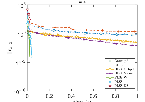
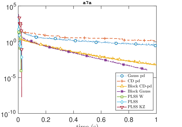
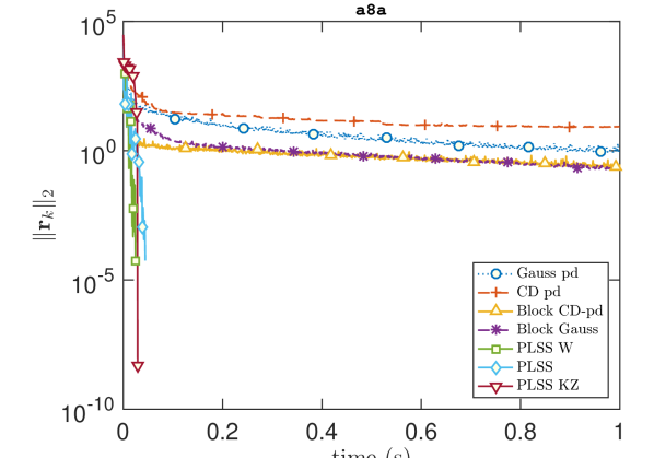
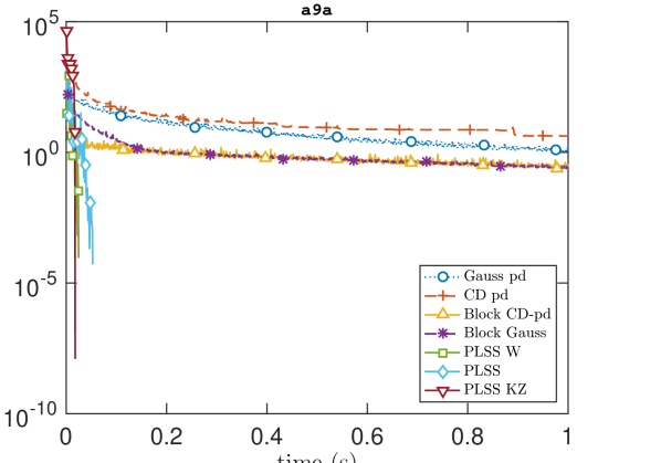
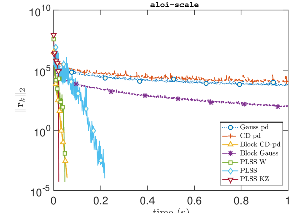
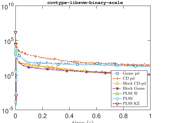
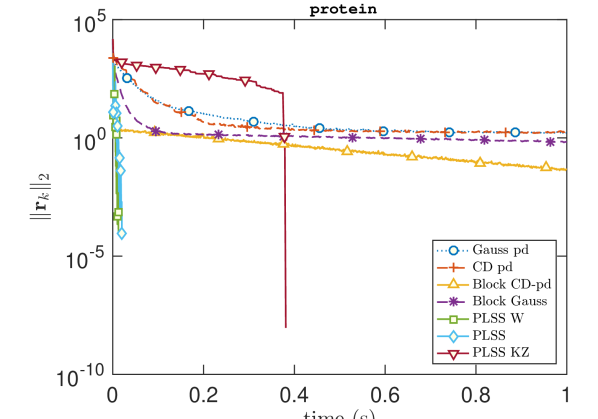
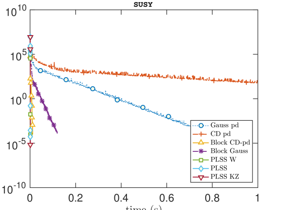
Figure 1: Comparison with randomized projection methods over a time interval of 1 second. The error represents the 2-norm of residuals. Four implementations of [6] are included for reference.

8.6 Randomized projection

For further comparison of our methods with randomized projections, we use the unsymmetric ill-conditioned ‘sampling’ matrix from MATLAB’s matrix gallery with n = 100; A = gallery(‘sampling’,n). The solution is the vector of all ones, and $\mathbf{x}_{0}=\mathbf{0}$. For this problem, cond(A) = 2.7859e+17. In Figure 2 we compare Algorithm 1 (with $\mathbf{W}=\mathbf{I}$) to updates (8) with random normal sketching matrices and varying dimensions of the sketch (i.e., $r$ varies). As expected, the convergence behavior of the randomized methods improves when $r$ increases from 10 to 40. At the same time, PLSS uses a simple recursive update (with very low computational cost) and converges significantly more rapidly than any of the random sketches.

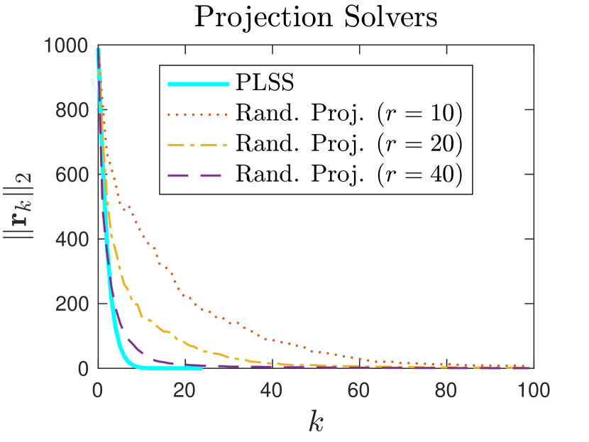
Figure 2: Comparison of PLSS with random normal projected solvers when the size of the sketch increases: $r=10,20,40$.

9 Conclusions

We develop an iterative projection method for solving consistent rectangular or square systems. Our method is based on appending one column each iteration to the sketching matrix. For full-rank sketches (common in practice) we prove that the underlying process terminates, with exact arithmetic, in a finite number of iterations. When the sketching matrix stores the history of all previous residuals, we develop a method with orthogonal residuals and updates. We include a parameter matrix that can be used to improve computations. Importantly, we derive a short recursive formula that is simple to implement, and an algorithm that updates only four vectors. In numerical experiments, including large sparse systems, our methods compare favorably to widely known methods (LSQR, LSMR or CRAIG) and to some existing randomized methods.

Appendix A Optimality

Solving linear system (5) is equivalent to the constrained optimization problem

(41) $$\min_{\mathbf{p}\in\mathbb{R}^{n}}\quad \frac{1}{2}\|\mathbf{B}\mathbf{p}\|^{2}_{2}-\mathbf{r}_{k-1}^{\top}\mathbf{A}\mathbf{p}$$

(42) subject to $${\color[rgb]{0,0,0}\mathbf{S}^{\top}_{k}}\mathbf{A}({\color[rgb]{0,0,0}\mathbf{x}_{k-1}}+\mathbf{p})={\color[rgb]{0,0,0}\mathbf{S}^{\top}_{k}}\mathbf{b}.$$

When $\mathbf{S}_{k}\in\mathbb{R}^{n\times k}$ is in the range of $\mathbf{A}=\mathbf{U}{\boldsymbol{\Sigma}}\mathbf{V}^{\top}$, it can be represented as $\mathbf{S}_{k}=\mathbf{U}\mathbf{T}_{k}$ using a nonsingular matrix $\mathbf{T}_{k}\in\mathbb{R}^{k\times k}$. Thus constraint (42) implies

$${\boldsymbol{\Sigma}}\mathbf{V}^{\top}(\mathbf{x}_{k-1}+\mathbf{p})=\mathbf{U}^{\top}\mathbf{b}\quad\text{ or }\quad\mathbf{A}\mathbf{p}=\mathbf{U}\mathbf{U}^{\top}\mathbf{r}_{k-1,}$$

with $\mathbf{r}_{k-1}=\mathbf{b}-\mathbf{A}\mathbf{x}_{k-1}$. Since $\mathbf{r}_{k-1}^{\top}\mathbf{A}\mathbf{p}=\|\mathbf{U}^{\top}\mathbf{r}_{k-1}\|^{2}_{2}$ is constant with respect to $\mathbf{p}$, problem (41)–(42) is equivalently represented by

$$\min_{\mathbf{p}\in\mathbb{R}^{n}}\quad \frac{1}{2}\|\mathbf{B}\mathbf{p}\|^{2}_{2}$$

subject to $${\color[rgb]{0,0,0}\mathbf{S}^{\top}_{k}}\mathbf{A}({\color[rgb]{0,0,0}\mathbf{x}_{k-1}}+\mathbf{p})={\color[rgb]{0,0,0}\mathbf{S}^{\top}_{k}}\mathbf{b}.$$

Appendix B Linear combination of updates

We derive a representation of $\mathbf{p}_{{\color[rgb]{0,0,0}k}}$ as a linear combination of previous updates ${\mathbf{p}}_{{\color[rgb]{0,0,0}k-1}},\ldots,{\mathbf{p}}_{1}$. Recall from (17) that

$$\mathbf{p}_{{\color[rgb]{0,0,0}k}}=\frac{{\color[rgb]{0,0,0}{\color[rgb]{0,0,0}\mathbf{s}_{k}}^{\top}\mathbf{r}_{k-1}}}{\delta_{{\color[rgb]{0,0,0}k}}}\left(\mathbf{y}_{{\color[rgb]{0,0,0}k}}-\mathbf{Y}_{k-1}\widehat{{\mathbf{t}}}_{k}\right),$$

where

$$\widehat{{\mathbf{t}}}_{k}={\mathbf{R}}_{k-1}{\mathbf{D}}_{k-1}{\mathbf{R}}_{k-1}^{\top}{\mathbf{Y}}_{k-1}^{\top}\mathbf{y}_{{\color[rgb]{0,0,0}k}}=\bigg{(}\begin{bmatrix}{\mathbf{R}}_{k-2}{\mathbf{D}}_{k-2}{\mathbf{R}}_{k-2}^{\top}&\\ &0\end{bmatrix}+\frac{{\mathbf{{\color[rgb]{0,0,0}t}}}_{{\color[rgb]{0,0,0}k-1}}{\mathbf{{\color[rgb]{0,0,0}t}}}_{{\color[rgb]{0,0,0}k-1}}^{\top}}{\delta_{k-1}}\bigg{)}{\mathbf{Y}}_{k-1}^{\top}\mathbf{y}_{{\color[rgb]{0,0,0}k}}$$

(with superscript indices suppressed). From this we deduce

$${\mathbf{Y}}_{k-1}\widehat{{\mathbf{t}}}_{k} ={\mathbf{Y}}_{k-2}{\mathbf{R}}_{k-2}{\mathbf{D}}_{k-2}{\mathbf{R}}_{k-2}^{\top}{\mathbf{Y}}_{k-2}^{\top}\mathbf{y}_{{\color[rgb]{0,0,0}k}}+\frac{{\mathbf{t}}_{k-1}^{\top}({\mathbf{Y}}_{k-1}^{\top}\mathbf{y}_{{\color[rgb]{0,0,0}k}})}{\delta_{k-2}}{\mathbf{Y}}_{k-1}{\mathbf{t}}_{k-1}$$

$$={\mathbf{Y}}_{k-2}{\mathbf{R}}_{k-2}{\mathbf{D}}_{k-2}{\mathbf{R}}_{k-2}^{\top}{\mathbf{Y}}_{k-2}^{\top}\mathbf{y}_{{\color[rgb]{0,0,0}k}}+\frac{{\mathbf{t}}_{k-1}^{\top}({\mathbf{Y}}_{k-1}^{\top}\mathbf{y}_{{\color[rgb]{0,0,0}k}})}{\delta_{k-1}}({\mathbf{Y}}_{k-2}\widehat{{\mathbf{t}}}_{k-1}-{\mathbf{y}}_{k-1})$$

$$={\mathbf{Y}}_{k-2}{\mathbf{R}}_{k-2}{\mathbf{D}}_{k-2}{\mathbf{R}}_{k-2}^{\top}{\mathbf{Y}}_{k-2}^{\top}\mathbf{y}_{{\color[rgb]{0,0,0}k}}-\frac{({\mathbf{t}}_{k-1}^{\top}({\mathbf{Y}}_{k-1}^{\top}\mathbf{y}_{{\color[rgb]{0,0,0}k}}))}{{\color[rgb]{0,0,0}\mathbf{s}_{k-1}^{\top}\mathbf{r}_{k-2}}}{\mathbf{p}}_{k-1}.$$

Now for $j=1\!:\!k-1$, define scalars $\alpha_{j}={\mathbf{t}}_{j}^{\top}({\mathbf{Y}}_{j}^{\top}\mathbf{y}_{{\color[rgb]{0,0,0}k}})/{\color[rgb]{0,0,0}(\mathbf{s}_{j}^{\top}\mathbf{r}_{j-1})}$, so that writing ${\mathbf{R}}_{k-2}{\mathbf{D}}_{k-2}{\mathbf{R}}_{k-2}$ in terms of ${\mathbf{R}}_{k-3}{\mathbf{D}}_{k-3}{\mathbf{R}}_{k-3}$ and ${\mathbf{t}}_{k-2}$ (and recursively backwards) gives

$${\mathbf{Y}}_{k-1}\widehat{{\mathbf{t}}}_{k}=-\sum_{j=1}^{k-1}\alpha_{j}{\mathbf{p}}_{j}.$$

Hence the update $\mathbf{p}_{{\color[rgb]{0,0,0}k}}$ can be represented by previous updates and the vector $\mathbf{y}_{{\color[rgb]{0,0,0}k}}$:

$$\mathbf{p}_{{\color[rgb]{0,0,0}k}}=\frac{{\color[rgb]{0,0,0}{\color[rgb]{0,0,0}\mathbf{s}_{k}}^{\top}\mathbf{r}_{k-1}}}{\delta_{{\color[rgb]{0,0,0}k}}}\left(\mathbf{y}_{{\color[rgb]{0,0,0}k}}-\mathbf{Y}_{k-1}\widehat{{\mathbf{t}}}_{k}\right)=\frac{{\color[rgb]{0,0,0}{\color[rgb]{0,0,0}\mathbf{s}_{k}}^{\top}\mathbf{r}_{k-1}}}{\delta_{k}}\big{(}{\color[rgb]{0,0,0}\mathbf{y}_{k}}+\sum_{j=1}^{k-1}\alpha_{j}{\mathbf{p}}_{j}\big{)}.$$

Appendix C Condition numbers

The condition numbers for the problems in Tables 1, 2 and 4 are shown in Table 5.

Table 5: Condition numbers $\kappa$ for the matrices in Tables 1, 2 and 4. Matrices in the first 7 rows correspond to Tables 1 and 2. Those in rows 8–14 correspond to Table 4.

Matrix $\kappa$ Matrix $\kappa$ Matrix $\kappa$ Matrix $\kappa$ Matrix $\kappa$ Matrix $\kappa$ lpi_gran 4e+13 landmark 1e+08 Kemelmacher 2e+04 Maragal_4 9e+06 Maragal_5 5e+12 Franz4 5 Franz5 1e+01 Franz6 8 Franz7 5 Franz8 6 Franz9 6 Franz10 6 GL7d12 8 GL7d13 1e+10 ch6-6-b3 2 ch7-6-b3 2 ch7-8-b2 1 ch7-9-b2 1 ch8-8-b2 1 cis-n4c6-b3 1 cis-n4c6-b4 1 mk10-b3 2 mk11-b3 2 mk12-b2 1 n2c6-b4 1 n2c6-b5 1 n2c6-b6 2 n3c6-b4 1 n3c6-b5 1 n3c6-b6 1 n4c5-b4 1 n4c5-b5 2 n4c5-b6 2 n4c6-b3 1 n4c6-b4 1 rel7 1e+01 relat7b 1e+01 relat7 1e+01 mesh_deform 1e+03 162bit 1e+03 176bit 3e+03 specular 3e+08 lp_25fv47 3e+03 lp_bnl1 3e+03 lp_bnl2 8e+03 lp_cre_a 2e+04 lp_cre_c 2e+04 lp_cycle 1e+07 lp_czprob 9e+03 lp_d2q06c 1e+05 lp_d6cube 1e+03 lp_degen3 8e+02 lp_fffff800 1e+10 lp_finnis 1e+03 lp_fit1d 5e+03 lp_fit1p 7e+03 lp_ganges 2e+04 lp_gfrd_pnc 9e+04 lp_greenbea 4e+03 lp_greenbeb 4e+03 lp_ken_07 1e+02 lp_maros 2e+06 lp_maros_r7 2 lp_modszk1 4e+01 lp_pds_02 4e+01 lp_perold 5e+05 lp_pilot 3e+03 lp_pilot4 4e+05 lp_pilot87 8e+03 lp_pilot_ja 3e+08 lp_pilot_we 5e+05 lp_pilotnov 4e+09 lp_qap12 3 lp_qap8 3 lp_scfxm2 2e+04 lp_scfxm3 2e+04 lp_scrs8 9e+04 lp_scsd6 9e+01 lp_scsd8 1e+03 lp_sctap2 2e+02 lp_sctap3 2e+02 lp_shell 4e+01 lp_ship04l 1e+02 lp_ship04s 1e+02

References

- [1] N. Ailon and B. Chazelle, The fast Johnson–Lindenstrauss transform and approximate nearest neighbors, SIAM J. Computing, 39 (2009), pp. 302–322.
- [2] J. J. Brust, Code for Algorithm PLSS and test programs. https://github.com/johannesbrust/PLSS, 2022.
- [3] C.-C. Chang and C.-J. Lin, LIBSVM: A library for support vector machines, ACM Trans. on Intelligent Systems and Technology (TIST), 2 (2011), pp. 1–27.
- [4] T. A. Davis, Y. Hu, and S. Kolodziej, SuiteSparse matrix collection. https://sparse.tamu.edu/, 2015–present.
- [5] G. H. Golub and C. F. Van Loan, Matrix Computations, The Johns Hopkins University Press, Baltimore, Maryland, third ed., 1996.
- [6] R. M. Gower and P. Richtárik, Randomized iterative methods for linear systems, SIAM J. Matrix Anal. Appl., 36 (2015), pp. 1660–1690, https://doi.org/10.1137/15M1025487, https://doi.org/10.1137/15M1025487.
- [7] N. Halko, P. Martinsson, and J. Tropp, Finding structure with randomness: Probabilistic algorithms for constructing approximate matrix decompositions, SIAM Review, 53 (2011), pp. 217–288, https://doi.org/10.1137/090771806.
- [8] W. Johnson and J. Lindenstrauss, Extensions of Lipschitz maps into a Hilbert space, Contemporary Mathematics, 26 (1984), pp. 189–206, https://doi.org/10.1090/conm/026/737400.
- [9] S. Kaczmarz, Angenaeherte aufloesung von systemen linearer gleichung, Bull. Internat. Acad. Polon. Sci. Lettres A, (1937), pp. 335–357.
- [10] D. M. Kane and J. Nelson, Sparser Johnson–Lindenstrauss transforms, J. Association for Computing Machinery, 61 (2014), pp. 1–23.
- [11] D. Leventhal and A. S. Lewis, Randomized methods for linear constraints: convergence rates and conditioning, Mathematics of Operations Research, 35 (2010), pp. 641–654.
- [12] C. C. Paige, Bidiagonalization of matrices and solution of linear equations, SIAM J. Numer. Anal., 11 (1974), pp. 197–209.
- [13] C. C. Paige and M. A. Saunders, LSQR: An algorithm for sparse linear equations and sparse least squares, ACM Trans. Math. Softw., 8 (1982), pp. 43–71, https://doi.org/10.1145/355984.355989, https://doi.org/10.1145/355984.355989.
- [14] C. C. Paige and M. A. Saunders, CRAIG: Sparse equations. http://stanford.edu/group/SOL/software/craig/, 2014–2022.
- [15] Z. Qu, P. Richtárik, M. Takác, and O. Fercoq, SDNA: Stochastic dual Newton ascent for empirical risk minimization, in International Conference on Machine Learning, 2016, pp. 1823–1832.
- [16] P. Richtárik and M. Takáč, Stochastic reformulations of linear systems: Algorithms and convergence theory, SIAM J. Matrix Anal. Appl., 41 (2020), pp. 487–524, https://doi.org/10.1137/18M1179249, https://doi.org/10.1137/18M1179249, https://arxiv.org/abs/https://doi.org/10.1137/18M1179249.
- [17] T. Strohmer and R. Vershynin, A randomized Kaczmarz algorithm with exponential convergence, J. Fourier Anal. Appl., 15 (2009), https://doi.org/10.1007/s00041-008-9030-4.