Negative energy effects in processes involving bound particles: finite nuclear size effects

Abstract

Probability of finding negative energy states in a hydrogen atom is decreased when the nucleus is extended. Reduced electron Compton wavelength is the characteristic size of the region around the nucleus where negative energy contributions to the wave function are sizeable.

1 Introduction

The hydrogen atom consists most of the time of a nucleus and a single electron. There is, however, a small probability that additional electron-positron pairs appear. Positrons are represented by negative-energy solutions of the Dirac equation. The probability of finding negative-energy components of the wave function was first determined by Bethe [1]. In the ground state of a hydrogen-like ion with the atomic number $Z$ that probability is

$$P_{-}\left(Z\right)=\frac{8\alpha_{Z}^{5}}{15\pi},$$ (1)

where $\alpha_{Z}=Z\alpha$ and $\alpha\simeq 1/137$ is the fine structure constant. Eq. (1) applies in the case of a point-like nucleus. Here we demonstrate that in the case of an extended charge distribution in the nucleus, this probability $P_{-}$ decreases. This is interpreted as follows. Negative energy states appear mainly in the region of a strong potential, in analogy with the Klein paradox [2, 3, 4]. When the nucleus is extended, the region of the strong potential is removed.

In the present work we focus on hydrogen-like ions containing spin-1/2 electrons. Ions with bound spin-0 particles have recently been considered in [5], in the limit of a point-like nucleus. For an excellent review of a variety of bound-state phenomena, see for example Ref. [6].

2 Models of an extended nucleus

2.1 Spherical shell

Instead of the whole charge $Ze$ concentrated in a point, we consider a uniform surface charge distribution on a spherical shell of radius $R$. The reason why we choose this particular model is that it is easy to treat analytically. Besides, the details of the charge distribution are not important for us. All we want to determine is how the probability of finding negative energy states decreases in the absence of the region of a very strong field. Inside a spherical shell there is no field at all and we can change the field outside by changing the radius $R$ of the shell.

We use such units that $\hbar=c=\epsilon_{0}=1$. Then the electrostatic potential energy of an electron interacting with the shell is ([7], Chapter 15)

$$V_{\text{shell}}\left(r\right)=\begin{cases}-\frac{\alpha_{Z}}{R}&r<R,\\ -\frac{\alpha_{Z}}{r}&r>R.\end{cases}$$ (2)

This function has a Fourier transform that is easy to remember: it is similar to the Fourier transform of the Coulomb potential, $V_{\text{C}}\left(k\right)=-4\pi\alpha_{Z}/k^{2}$, but it is modulated by the sinc function,

$$V_{\text{shell}}\left(k\right)=V_{\text{C}}\left(k\right)\cdot\frac{\sin\kappa}{\kappa},\quad\kappa=kR.$$ (3)

In the limit $R\to 0$ we reproduce the Coulomb potential of a pointlike nucleus.

2.2 Uniformly charged ball

Although we will be using the spherical shell model, here we introduce a uniformly charged sphere as an alternative charge distribution,

$$\rho\left(r\right)=\begin{cases}\text{constant}&r<R,\\ 0&r>R.\end{cases}$$ (4)

Our goal is to demonstrate that the Fourier spectrum of the potential is similar in both cases, strengthening the argument that the details of the charge distribution are not decisive for our conclusions. Electron’s potential energy resulting from the interaction with the density in Eq. (4) is

$$V_{\text{ball}}\left(r\right)=\begin{cases}-\frac{\alpha_{Z}}{R}\left(\frac{5}{4}-\frac{r^{4}}{4R^{4}}\right)&r<R,\\ -\frac{\alpha_{Z}}{r}&r>R.\end{cases}$$ (5)

Its Fourier transform is

$$V_{\text{ball}}\left(k\right)=5V_{\text{C}}\left(k\right)\cdot\frac{3\left(\kappa^{2}-2\right)\sin\kappa-\kappa\left(\kappa^{2}-6\right)\cos\kappa}{\kappa^{5}},\quad\kappa=kR.$$ (6)

Fourier transforms of both the shell and the solid ball potentials, normalized to the Coulomb potential, are shown in Figure 1.

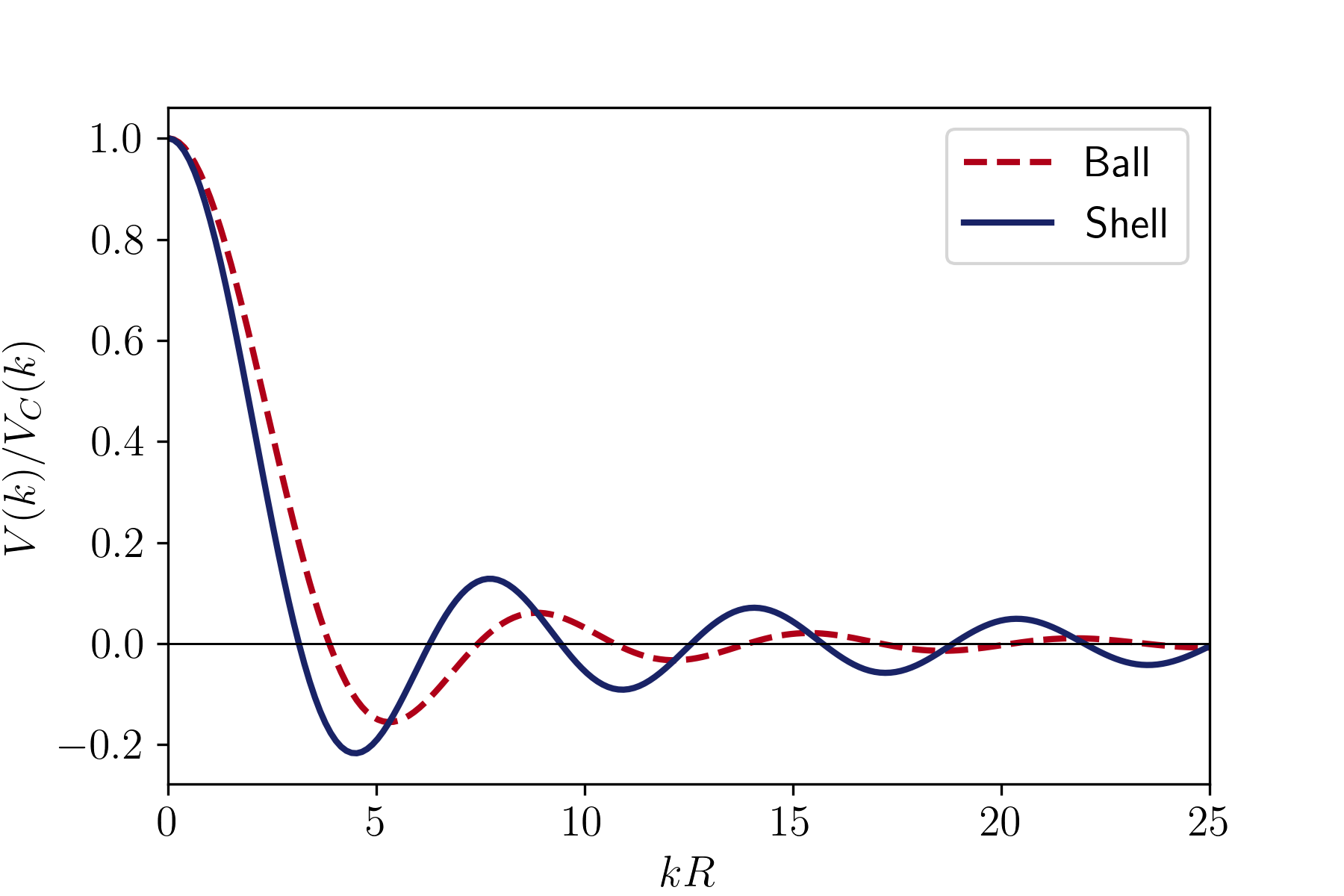
Figure 1: Fourier transforms of electron’s potential energy due to its interaction with two charge distributions: a solid ball (red, dashed) and a hollow shell (blue, solid), normalized to the Coulomb potential of a point-like distribution. For a given radius of the charge distribution, the two Fourier transforms are similar. In both cases, the smearing of the charge decreases the magnitude of high-momentum (large $kR$) Fourier components.

3 Negative energy states in the case of an extended nucleus

In order to find the probability $P_{-}\left(Z\right)$ of finding negative energy states in the potential of Eq. (3), we need the negative energy component of the wave function $\phi_{-}\left(\bm{k}\right)$. Once that is determined, the needed probability is

$$P_{-}\left(Z\right)=\int\frac{\mbox{d}^{3}k}{\left(2\pi\right)^{3}}\left|\phi_{-}\left(\bm{k}\right)\right|^{2}.$$ (7)

That wave function component satisfies an integral equation, derived from the Fourier transform of the Dirac equation [8]. That equation is greatly simplified in the approximation where $\phi_{-}\left(\bm{k}\right)$ is small and can be neglected under the integral [1, 5]. In the case of the hollow shell potential in Eq. (3) one finds

$$\phi_{-}\left(\bm{k}\right)=-\frac{4\pi\alpha_{Z}}{\left(m+E\right)k^{2}}\frac{\sin kR}{kR}\sqrt{\frac{E-m}{2E}}\psi\left(0\right)$$ (8)

where $E=\sqrt{m^{2}+k^{2}}$, $m$ is the electron mass, and the wave function at the origin is approximately $\psi\left(0\right)\simeq 1/\sqrt{\pi a^{3}}$, where $a=1/\left(m\alpha_{Z}\right)$ is the Bohr radius. The negative energy probability can now be calculated,

$$P_{-}\left(Z\right)=\frac{4\alpha_{Z}^{5}m^{3}}{\pi R^{2}}\int_{0}^{\infty}\mbox{d}k\frac{\sin^{2}kR}{E\left(E+m\right)^{4}\left(E-m\right)}.$$ (9)

Introduce a new variable $\epsilon$, $E=\epsilon m$, $k\mbox{d}k=m^{2}\epsilon\mbox{d}\epsilon$, and denote $mR$ by $\mu$,

$$P_{-}\left(Z\right)=\frac{4\alpha_{Z}^{5}}{\pi\mu^{2}}J,\qquad J=\int_{1}^{\infty}\mbox{d}\epsilon\frac{\sin^{2}\left(\sqrt{\epsilon^{2}-1}\mu\right)}{\left(\epsilon+1\right)^{9/2}\left(\epsilon-1\right)^{3/2}},\qquad\mu=mR.$$ (10)

When the radius $R$ of the charge distribution is large in comparison with the reduced Compton wavelength of the electron $1/m$, $\mu$ is large, the sine function in the numerator oscillates rapidly, and its square could in some integrands be replaced by $1/2$. In our present case, this does not work because in the region $\epsilon-1\ll 1$ the square root factor in the argument of the sine compensates the large value of $\mu$. Thus we first add and subtract a simpler function that has a similar behavior for $\epsilon$ near 1,

$$J=\int_{1}^{\infty}\mbox{d}\epsilon\left\{\frac{\sin^{2}\left(\sqrt{\epsilon^{2}-1}\mu\right)}{\left(\epsilon+1\right)^{9/2}\left(\epsilon-1\right)^{3/2}}-\frac{\sin^{2}\left[\sqrt{2}\sqrt{\epsilon-1}\mu\right]}{2^{9/2}\left(\epsilon-1\right)^{3/2}}+\frac{\sin^{2}\left[\sqrt{2}\sqrt{\epsilon-1}\mu\right]}{2^{9/2}\left(\epsilon-1\right)^{3/2}}\right\}.$$ (11)

In the first two terms we replace the sine-squared factors by 1/2; this eliminates the dependence of these terms on $\mu$, they become subleading for large $\mu$ and can be neglected. The last term, evaluated analytically, gives

$$P_{-}\left(Z\right)\xrightarrow{\mu\gg 1}\frac{\alpha_{Z}^{5}}{4\mu}.$$ (12)

We see that the probability of negative energy contributions decreases with the radius of the charge distribution, confirming the intuition that these contributions arise in the region of a strong potential.

Subleading terms in Eq. (11) introduce a small negative term. Including them significantly increases the range of $\mu$ over which the large-$\mu$ asymptotics agrees with the exact $J$,

$$P_{-}\left(Z\right)\xrightarrow{\mu\gg 1}\alpha_{Z}^{5}\left(\frac{1}{4\mu}-\frac{16}{35\pi\mu^{2}}\right).$$ (13)

For completeness, we determine the behavior of $J$ for small $\mu$. The sine function can be replaced by the first two terms of its Taylor expansion. We retain only the square of the leading term and its product with the subleading term and find

$$P_{-}\left(Z\right)\xrightarrow{\mu\ll 1}\frac{4\alpha_{Z}^{5}}{45\pi}\left(6-5\mu^{2}\right).$$ (14)

When $\mu\to 0$, this reproduces Bethe’s result [1]. Both the large and small $R$ asymptotics of $P_{-}\left(Z\right)$ are plotted in Figure 2.

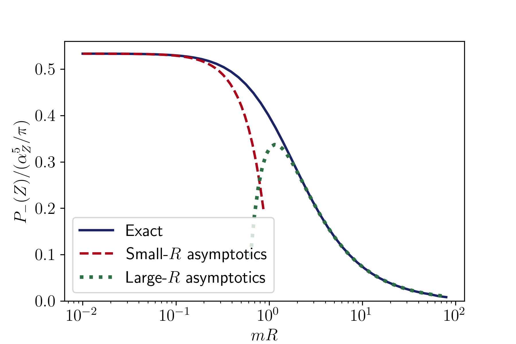
Figure 2: Probability of finding negative energy states in an hydrogen-like ion with an extended nucleus: a shell of radius $R$. The solid blue curve shows the numerical integral as in Eq. (10). For $R$ small in comparison with the electron’s reduced Compton wavelength (red, dashed line defined by Eq. (14)), the result approaches Bethe’s value of Eq. (1), with $8/15\simeq 0.53$. For large $R$ (greed, dotted line defined by Eq. (12)), negative energy states are suppressed because the potential is weak.

4 Conclusions

Finite size of the nucleus removes the region where the potential is very strong. This decreases the probability of finding negative energy components in the electron wave function. For large radii of the charge distribution the decrease is linear in the ratio of the the electron’s reduced Compton wavelength to the nuclear radius.

References

- [1] H. A. Bethe, Bemerkungen über die Wasserstoff-Eigenfunktionen in der Diracschen Theorie, Zeitschrift für Naturforschung A 3, 470 – 477 (1948).
- [2] O. Klein, Die Reflexion von Elektronen an einem Potentialsprung nach der relativistischen Dynamik von Dirac, Zeitschrift für Physik 53, 157–165 (1929).
- [3] B. R. Holstein, Klein’s paradox, Am. J. Phys. 66, 507–512 (1998).
- [4] A. Hansen and F. Ravndal, Klein’s Paradox and Its Resolution, Physica Scripta 23, 1036–1042 (1981).
- [5] A. Czarnecki, Negative Energy States in Pionic Hydrogen, Acta Phys. Polon. Supp. 15, 1 (2022), 2202.03538.
- [6] P. Hoyer, Journey to the Bound States, SpringerBriefs in Physics, Springer (2021), 2101.06721.
- [7] S. Chandrasekhar, Newton’s Principia for the Common Reader, Clarendon Press (2003).
- [8] H. Feshbach and F. Villars, Elementary relativistic wave mechanics of spin 0 and spin 1/2 particles, Rev. Mod. Phys. 30, 24–45 (1958).