Negative energy states in pionic hydrogen

Abstract

Probabilities of finding an antiparticle in an atom or ion containing a particle of spin 1/2 or spin 0 are determined. The spin 1/2 case was previously solved by Hans Bethe and his work is summarized. The spin 0 case is treated numerically for an arbitrary atomic number and analytically for small atomic numbers. The main tool for the spin 0 case is the Feshbach-Villars representation of the Klein-Gordon equation.

1 Introduction

Solution of a Dirac equation with a Coulomb potential has a well-defined energy, equal to the electron rest energy decreased by the binding, which amounts to about $13.6$ eV in case of hydrogen. However, a decomposition of the full solution of the Dirac equation into plane waves contains both positive and negative energy solutions of the free Dirac equation. Positive energy solutions alone do not form a complete basis. Negative energy components, describing antiparticles resulting from the virtual pair production, contribute very little to the norm of the wave function, only a fraction of a percent even for heavy ions like the hydrogen-like lead with the atomic number $Z=82$. For smaller $Z$, this contribution decreases further and for small $\alpha_{Z}=Z\alpha$, where $\alpha\simeq 1/137$ denotes the fine structure constant, becomes approximately $8\alpha_{Z}^{5}/(15\pi)$ [1] in the ground state. Throughout this paper we focus on the ground state only.

Despite the smallness of their contribution to the norm, the negative energy states have been found to contribute significantly to some processes, on par with positive energies. For example, when a muon bound in an atom decays, there is some probability that the resulting electron remains bound. In this process, negative energy components of the muon and of the electron wave functions play an important role [2, 3]. This is counterintuitive. For example, in an earlier study of the bound muon decay, these negative-energy contributions were neglected, which led to a significant error [4].

How large are negative energy contributions in the case of a spinless particle like a pion, bound in a hydrogen-like atom? In the present paper, this question is answered. This study is motivated by experiments with pionic atoms carried out at the Paul Scherrer Institute [5, 6]. We find that the probability of finding an antipion in a pionic atom is $2\alpha_{Z}^{5}/(15\pi)$, a factor of 4 smaller than in the fermionic case.

Section 2 reviews Bethe’s work on antiparticles in the Dirac equation. In Section 3 we summarize a two-component wave function formalism for the Klein-Gordon equation which makes the negative energy contributions explicit. Probability of finding antiparticles is computed numerically using the momentum-space wave function (Subsection 3.1). An analytic result is found for small $\alpha_{Z}$ using an integral equation for the wave function (Subsection 3.2). Section 4 contains conclusions. An appendix reviews solutions of the Schrödinger and the Klein-Gordon equations with a Coulomb potential and summarizes our convention for Laguerre polynomials.

2 Negative energy content: the case of spin 1/2

2.1 Integral Dirac equation

Let $\psi\left(\bm{r}\right)$ be the spinor wave function of an electron in the ground state of a hydrogen-like ion, with spin up. Define its Fourier component $\phi\left(\bm{k},\tau\right)$ with spin projection $\tau$ (with units such that $\hbar=c=1$),

$$\psi\left(\bm{r}\right)=\sum_{\tau}\int\frac{\mbox{d}^{3}k}{\left(2\pi\right)^{3}}\phi\left(\bm{k},\tau\right)u_{\tau}\left(\bm{k}\right)e^{i\bm{k}\cdot\bm{r}}.$$ (1)

$u_{\tau}$ are spatially-constant Dirac amplitudes for a free electron normalized by $u_{\sigma}^{\dagger}u_{\tau}=\delta_{\sigma\tau}$,

$$u_{1,2}\left(\bm{k}\right) =\sqrt{\frac{E+m}{2E}}\left(\begin{array}[]{c}\varphi_{\pm}\\ \frac{\bm{\sigma}\cdot\bm{k}}{E+m}\varphi_{\pm}\end{array}\right),\qquad\varphi_{+}=\left(\begin{array}[]{c}1\\ 0\end{array}\right),\quad\varphi_{-}=\left(\begin{array}[]{c}0\\ 1\end{array}\right),$$ (8)

$$u_{3,4}\left(\bm{k}\right) =\sqrt{\frac{E+m}{2E}}\left(\begin{array}[]{c}\pm\frac{\bm{\sigma}\cdot\bm{k}}{E+m}\varphi_{\mp}\\ \mp\varphi_{\mp}\end{array}\right),\quad E=\sqrt{m^{2}+k^{2}},\quad k=|\bm{k}|.$$ (11)

They satisfy the Dirac equation in the following form,

$$\left(\bm{\alpha}\cdot\bm{k}+\beta m\right)u_{\sigma}\left(\bm{k}\right) =E_{\sigma}u_{\sigma}\left(\bm{k}\right),$$ (12)

$$E_{1,2} =E,\quad E_{3,4}=-E.$$ (13)

We are interested in small atomic numbers $Z$ such that $\alpha_{Z}\ll 1$. The dominant Fourier component is $\phi\left(\bm{k},1\right)$. The other positive energy component vanishes, $\phi\left(\bm{k},2\right)=0$, and components with $\tau=3,4$ describe the tiny negative energy content. All components are obtained by projection,

$$\phi\left(\bm{k},\sigma\right)=\int\mbox{d}^{3}re^{-i\bm{k}\cdot\bm{r}}\left[u_{\sigma}^{\dagger}\psi\left(\bm{r}\right)\right].$$ (14)

The integral form of the Dirac equation,

$$\left[V\left(r\right)+\bm{\alpha}\cdot\bm{k}+\beta m\right]\psi=W\psi,$$ (15)

is also derived with this projection. Here $V$ denotes the Coulomb potential energy, $V\left(r\right)=-\frac{\alpha_{Z}}{r}$, and $W$ is the total energy, $W\simeq m-\frac{\alpha_{Z}^{2}m}{2}$. If Eq. (15) is multiplied with $\int\mbox{d}^{3}re^{-i\bm{k}\cdot\bm{r}}u_{\sigma}^{\dagger}\left(\bm{k}\right)$, the first term becomes

$$V_{\sigma}^{\prime}(\bm{k}) =\int\mbox{d}^{3}re^{-i\bm{k}\cdot\bm{r}}\left[u_{\sigma}^{\dagger}\left(\bm{k}\right)\psi\left(\bm{r}\right)\right]V\left(\bm{r}\right)$$ (16)

$$=\int\frac{\mbox{d}^{3}q}{\left(2\pi\right)^{3}}\int\mbox{d}^{3}re^{-i\left(\bm{k}-\bm{q}\right)\cdot\bm{r}}\left[u_{\sigma}^{\dagger}\left(\bm{k}\right)\psi\left(\bm{r}\right)\right]\overbrace{\int\mbox{d}^{3}r^{\prime}e^{-i\bm{q}\cdot\bm{r}^{\prime}}V\left(\bm{r}^{\prime}\right)}^{V\left(\bm{q}\right)}$$ (17)

$$=\int\frac{\mbox{d}^{3}q}{\left(2\pi\right)^{3}}V\left(\bm{q}\right)\int\mbox{d}^{3}re^{-i\left(\bm{k}-\bm{q}\right)\cdot\bm{r}}\left[u_{\sigma}^{\dagger}\left(\bm{k}\right)\psi\left(\bm{r}\right)\right].$$ (18)

Substitute $\psi$ from Eq. (1),

$$V_{\sigma}^{\prime}(\bm{k}) =\int\frac{\mbox{d}^{3}q}{\left(2\pi\right)^{3}}V\left(\bm{q}\right)\sum_{\tau}\phi\left(\bm{k}-\bm{q},\tau\right)\underbrace{\left[u_{\sigma}^{\dagger}\left(\bm{k}\right)u_{\tau}\left(\bm{k}-\bm{q}\right)\right]}_{\left\langle\bm{k},\sigma|\bm{k}-\bm{q},\tau\right\rangle}.$$ (19)

The conjugate of (12) is $u_{\sigma}^{\dagger}\left(\bm{k}\right)\left(\bm{\alpha}\cdot\bm{k}+\beta m\right)=E_{\sigma}u_{\sigma}^{\dagger}\left(\bm{k}\right)$, so the last three terms of (15) give

$$\int\mbox{d}^{3}re^{-i\bm{k}\cdot\bm{r}}u_{\sigma}^{\dagger}\left(\bm{k}\right)\left(\bm{\alpha}\cdot\bm{k}+\beta m-W\right)\psi =\left[E_{\sigma}-W\right]\phi\left(\bm{k},\sigma\right).$$ (20)

Fourier-transforming the Coulomb potential, $\int\mbox{d}^{3}re^{-i\bm{q}\cdot\bm{r}}V\left(\bm{r}\right)$ $=-\frac{4\pi\alpha_{Z}}{q^{2}}$,

$$\left(W-E_{\sigma}\right)\phi\left(\bm{k},\sigma\right)=-4\pi\alpha_{Z}\int\frac{\mbox{d}^{3}q}{\left(2\pi\right)^{3}}\frac{1}{q^{2}}\sum_{\tau}\phi\left(\bm{k}-\bm{q},\tau\right)\left\langle\bm{k},\sigma|\bm{k}-\bm{q},\tau\right\rangle.$$ (21)

2.2 Solution of the Dirac equation for spin 1/2

In Eq. (21) set $W\simeq m$, $E_{\sigma}\left(\bm{k}\right)=-\sqrt{m^{2}+k^{2}}=-E$, and change the integration momentum $\bm{q}\to\bm{p}=\bm{k}-\bm{q}$

$$\left(m+E\right)\phi\left(\bm{k},\sigma\right)=-4\pi\alpha_{Z}\int\frac{\mbox{d}^{3}p}{\left(2\pi\right)^{3}}\frac{1}{\left(\bm{p}-\bm{k}\right)^{2}}\sum_{\tau}\phi\left(\bm{p},\tau\right)\left\langle\bm{k},\sigma|\bm{p},\tau\right\rangle.$$ (22)

In the first approximation, neglect $\bm{p}$ where possible, arguing that it introduces higher order corrections in $\alpha_{Z}$. Since the second spinor component of the spin-up wave function $\psi$ vanishes, form such a linear combination of $u_{3,4}$ in Eq. (11) that its second component is also zero, $u_{n}=\frac{1}{\sqrt{2E\left(E-m\right)}}\left(\begin{array}[]{c}E-m\\ 0\\ -k_{z}\\ -k_{+}\end{array}\right)$. Since the wave function in the momentum space is peaked at zero momentum, $\left(\bm{p}-\bm{k}\right)^{2}$ in the denominator can be approximated by $k^{2}$ and taken out of the integral. Also, neglecting corrections $\mathcal{O}\left(\bm{p}/m\right)$, only $\sigma=n$ and $\tau=1$ contribute, $\left\langle\bm{k},n|0,1\right\rangle=\sqrt{\left(E-m\right)/2E}$,

$$\phi_{-}\left(\bm{k}\right) \simeq-\frac{4\pi\alpha_{Z}}{\left(m+E\right)k^{2}}\sqrt{\frac{E-m}{2E}}\int\frac{\mbox{d}^{3}p}{\left(2\pi\right)^{3}}\phi\left(\bm{p},1\right)$$ (23)

$$=-\frac{4\pi\alpha_{Z}}{\left(m+E\right)k^{2}}\sqrt{\frac{E-m}{2E}}\psi\left(0\right),$$ (24)

where for the spatial wave function at the origin the non-relativistic result can be used, $\psi\left(\bm{r}=0\right)\simeq\sqrt{\frac{\alpha_{Z}^{3}m^{3}}{\pi}}$. This is the only characteristic of the wave function we need to determine the negative energy amplitude to the leading order in $\alpha_{Z}$. This reflects creation of particle-antiparticle pairs only in the vicinity of the origin, where the potential is strong. The resulting probability of finding negative energy states is

$$P_{-}(Z) =\int\frac{\mbox{d}^{3}k}{\left(2\pi\right)^{3}}\left|\phi_{-}(\bm{k})\right|^{2}$$ (25)

$$=4\frac{m^{3}\alpha_{Z}^{5}}{\pi}\int_{0}^{\infty}\mbox{d}kk^{2}\left[\frac{1}{\left(m+E\right)\left(E^{2}-m^{2}\right)}\sqrt{\frac{E-m}{E}}\right]^{2}.$$ (26)

Use $k\mbox{d}k=E\mbox{d}E$ and change variables to $E=m\epsilon$,

$$P_{-}(Z) =4\frac{\alpha_{Z}^{5}}{\pi}\int_{1}^{\infty}\frac{\mbox{d}\epsilon}{\left(\epsilon+1\right)^{7/2}\left(\epsilon-1\right)^{1/2}}=\frac{8\alpha_{Z}^{5}}{15\pi}.$$ (27)

This agrees with the numerical evaluation of $P_{-}(Z)$ presented in Fig. 1. Dots in that figure show $P_{-}/\alpha_{Z}^{4}$ from a numerical integration of the negative energy components of the exact solution of the Dirac equation with the Coulomb potential, obtained in [3]. When $Z$ is small, these dots come close to the straight line predicted by Eq. (27). However, already for $Z=8$, the straight line exceeds the numerical value by 59 per cent, even though $\left(Z=8\right)\cdot\alpha$ is less than $0.06$. Very likely higher-order effects in $\alpha_{Z}$, not included in Eq. (27), are logarithmically enhanced.

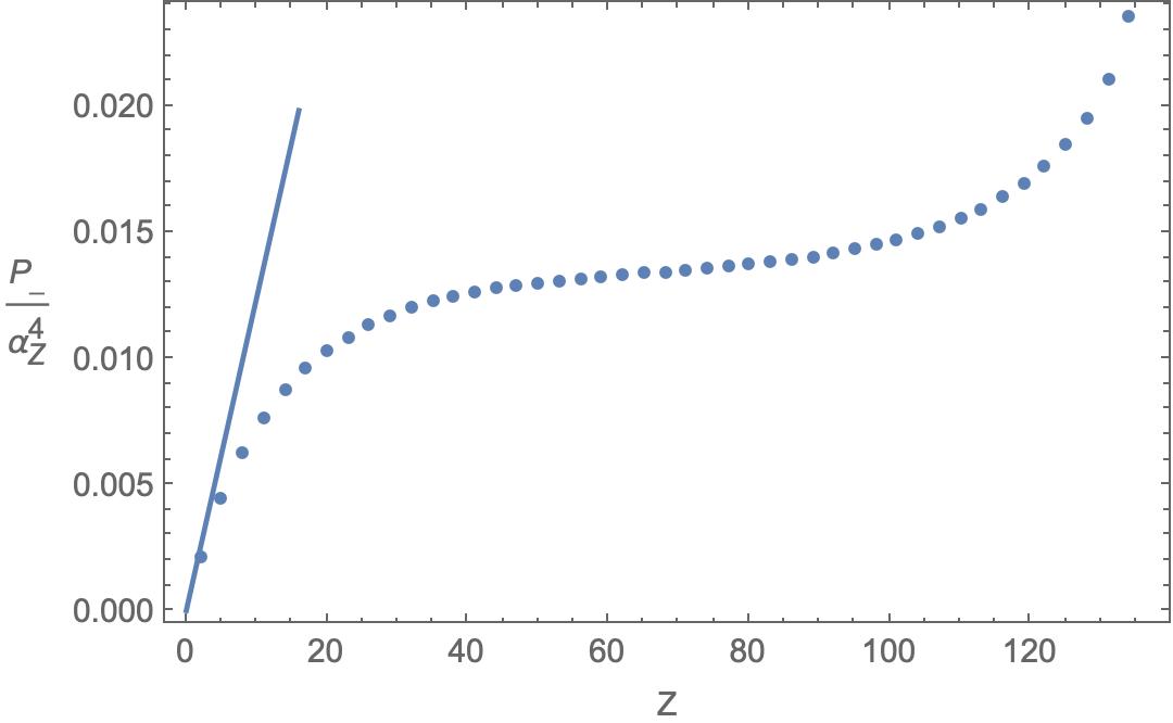
Figure 1: Probability of finding spin 1/2 electrons with negative energies, $P_{-}=\int\left(\left|\phi\left(\bm{p},3\right)\right|^{2}+\left|\phi\left(\bm{p},4\right)\right|^{2}\right)\frac{d^{3}p}{\left(2\pi\right)^{3}}$, divided by $\alpha_{Z}^{4}$, as a function of the atomic number $Z$, evaluated with $\phi\left(\bm{p},\sigma\right)$ computed in Ref. [3] (dots for every third integer $Z$). For $Z=5$ the value is about 0.004, in agreement with $\frac{8}{15\pi}\cdot 5\alpha=0.006$ predicted by Eq. (27). The first dot is for $Z=2$, just above 0.002, in even better agreement with $\frac{8}{15\pi}\cdot 2\alpha=0.0025$. When $Z\alpha\to 1$, $P_{-}$ seems to tend to 0.0329. The solid line shows the small $Z$ behavior predicted by Eq. (27).

3 Pionic atoms and the Klein-Gordon equation

We now proceed to an idealized description of a hydrogen-like ion with the electron replaced by a negative pion $\pi^{-}$, assumed to be point-like, stable, and not strongly interacting. The probability of negative energy components in its wave function is the spin 0 analogue of Eq. (27), which was derived for spin 1/2. We set out to derive it.

The spin 0 wave function is described by the Klein-Gordon (KG) equation. Decomposition of KG wave functions into plane waves with positive and negative energies was studied by Feshbach and Villars (FV) [7]. We shall first summarize the integral equation they derived and then solve it with the approximation method described in Section 2.2.

3.1 Feshbach-Villars representation of the KG wave function

Focus on the Coulomb problem with $V\left(r\right)=-\frac{\alpha_{Z}}{r}$ and no vector potential. The KG equation is

$$\left[\left(i\partial_{t}-V\right)^{2}+\nabla^{2}-m^{2}\right]\psi\left(\bm{r},t\right)=0.$$ (28)

The two component wave function, which we denote with a capital letter $\Psi$, satisfying a first-order equation in time, is

$$\Psi\left(\bm{r},t\right)=\left(\begin{array}[]{c}\phi\\ \chi\end{array}\right)=\frac{1}{\sqrt{2}m}\left(\begin{array}[]{c}m+i\partial_{t}-V\\ m-i\partial_{t}+V\end{array}\right)\psi\left(\bm{r},t\right).$$ (29)

The solution has the form $\Psi\left(\bm{r},t\right)=\Psi\left(\bm{r}\right)e^{-iWt}$ where $W$ is the energy eigenvalue. For the Coulomb problem $W=m-\frac{m\alpha_{Z}^{2}}{2}+\mathcal{O}\left(\alpha_{Z}^{4}\right)$. Assume that $W$ has been determined and focus on the time-independent part of the wave function. Use such units of energy that $m=1$. In momentum space,

$$\Psi\left(\bm{p}\right)=\int\mbox{d}^{3}re^{-i\bm{p}\cdot\bm{r}}\Psi\left(\bm{r}\right),$$ (30)

the wave function can be decomposed into plane waves with positive and negative energies,

$$\Psi\left(\bm{p}\right)=u\left(p\right)\Psi_{0}^{\left(+\right)}\left(\bm{p}\right)+v\left(p\right)\Psi_{0}^{\left(-\right)}\left(\bm{p}\right),\quad p=\left|\bm{p}\right|,$$ (31)

with $\Psi_{0}^{\left(\pm\right)}\left(\bm{p}\right)$ being an orthonormal basis, analogous to $u_{1,\dots,4}$ in Eqs. (8) and (11). This basis diagonalizes the free-particle Hamiltonian, explicitly decoupling positive and negative energy solutions (see Eq. (42)). Coefficients $u,v$ are related to $\phi,\chi$ by a unitary transformation; using $E_{p}=\sqrt{1+p^{2}}$,

$$\Psi^{\#}=\left(\begin{array}[]{c}u\left(p\right)\\ v\left(p\right)\end{array}\right)=U^{-1}\left(\begin{array}[]{c}\phi\left(p\right)\\ \chi\left(p\right)\end{array}\right),\,U^{-1}=\frac{1}{2\sqrt{E_{p}}}\left(\begin{array}[]{cc}E_{p}+1&E_{p}-1\\ E_{p}-1&E_{p}+1\end{array}\right).$$ (32)

Fourier components $\phi,\chi$ can be expressed in closed form, obtained from the configuration space wave function (see Appendix A),

$$\phi\left(p\right) =\phantom{-}a\left(p\right)\left(\sqrt{p^{2}+\nu}s_{1}+\frac{1-\nu+\sqrt{1-\nu}}{\sqrt{\nu}}s_{2}\right)$$ (33)

$$\chi\left(p\right) =-a\left(p\right)\left(\sqrt{p^{2}+\nu}s_{1}+\frac{1-\nu-\sqrt{1-\nu}}{\sqrt{\nu}}s_{2}\right)$$ (34)

$$a\left(p\right) =\frac{2^{1-\nu}\sqrt{\pi}\sqrt[4]{\nu\left(1-\nu\right)}\Gamma\left(1-\nu\right)}{p\sqrt{\Gamma\left(2-2\nu\right)}}\left(\frac{p^{2}+\nu}{\nu}\right)^{\frac{\nu}{2}-1},$$ (35)

$$s_{n=1,2} =\sin\left(\left(n-\nu\right)\arctan\frac{p}{\sqrt{\nu}}\right),\quad\nu=\frac{1}{2}-\sqrt{\frac{1}{4}-\alpha_{Z}^{2}}.$$ (36)

In the weak field limit when $\alpha_{Z}\ll 1$, $\nu$ is of order $\alpha_{Z}^{2}$ and so is the typical $p^{2}$. Then $\chi\ll\phi$ and $\chi$ is analogous to the small component of the Dirac wave function. Similarly, $v\ll u$. It is $v\left(p\right)$ that determines the probability $P_{-}$ of finding antiparticles,

$$P_{-}\left(Z\right)=\int\frac{\mbox{d}^{3}p}{\left(2\pi\right)^{3}}\left|v\left(p\right)\right|^{2}.$$ (37)

The result is plotted in Fig. 2 for $Z$ up to 68.

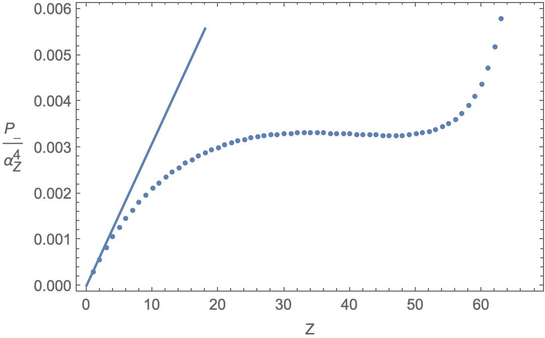
Figure 2: Probability of finding spin 0 particles with negative energies (the Klein-Gordon case), divided by $\alpha_{Z}^{4}$, as a function of the atomic number $Z$ (dots). Note that in the KG case, the field becomes supercritical at $\alpha_{Z}=1/2$ rather than 1 as in the Dirac case [8, 9]. The solid line shows the small $Z$ behavior in Eq. (38).

Note that for larger $Z$, when $\alpha_{Z}>1/2$, the field becomes supercritical [8, 9], unlike in the Dirac equation case which requires $\alpha_{Z}>1$ for super-criticality. For small $\alpha_{Z}$, numerical results plotted in Fig. 2 indicate the behavior

$$P_{-}\left(Z\to 0\right)=\frac{2\alpha_{Z}^{5}}{15\pi},$$ (38)

a four times smaller slope that in the Dirac equation case, Eq. (27). Eq. (38) can be confirmed analytically with the help of an integral equation, as we now proceed to demonstrate.

3.2 Integral KG equation

Following Feshbach and Villars, write down the first order equation for the wave function $\Psi^{\#}$ decomposed into free particle solutions, Eq. (32). In momentum space, position operator is represented by $i\bm{\nabla}_{p}$. Using $\tau_{2}=\begin{pmatrix}0&-i\\ i&0\end{pmatrix}$ and $\tau_{3}=\begin{pmatrix}1&0\\ 0&-1\end{pmatrix}$,

$$i\partial_{t}\Psi^{\#}=U^{-1}i\partial_{t}\Psi =U^{-1}\left\{\left(\tau_{3}+i\tau_{2}\right)\frac{\bm{p}^{2}}{2m}+\tau_{3}m+V\left(i\bm{\nabla}_{p}\right)\right\}U\Psi^{\#}.$$ (39)

With identities

$$U^{-1}\tau_{3}U =\frac{\left(E_{p}^{2}+1\right)\tau_{3}+\left(1-E_{p}^{2}\right)i\tau_{2}}{2E_{p}},$$ (40)

$$U^{-1}\tau_{2}U =\frac{\left(E_{p}^{2}+1\right)\tau_{2}+\left(E_{p}^{2}-1\right)i\tau_{3}}{2E_{p}},$$ (41)

the free-particle part of the Hamiltonian is diagonal,

$$U^{-1}\left[\left(\tau_{3}+i\tau_{2}\right)\frac{\bm{p}^{2}}{2}+\tau_{3}\right]U=E_{p}\tau_{3},$$ (42)

and the wave equation becomes

$$i\partial_{t}\Psi^{\#} =E_{p}\tau_{3}\Psi^{\#}+U^{-1}\left(\bm{p}\right)V\left(i\bm{\nabla}_{p}\right)U\left(\bm{p}\right)\Psi^{\#}\left(\bm{p}\right).$$ (43)

For the Coulomb potential,

$$i\partial_{t}\Psi^{\#}=E_{p}\tau_{3}\Psi^{\#}-4\pi\alpha_{Z}U^{-1}\left(\bm{p}\right)\int\frac{\mbox{d}^{3}q}{\left(2\pi\right)^{3}}\frac{U\left(\bm{q}\right)\Psi^{\#}\left(\bm{q}\right)}{\left(\bm{p}-\bm{q}\right)^{2}}.$$ (44)

We are interested in the equation for the lower component $v$. With $i\partial_{t}\to W$ and neglecting $v$ in the right hand side since $v\ll u$,

$$\left(W+E_{p}\right)v =-4\pi\alpha_{Z}\int\frac{\mbox{d}^{3}q}{\left(2\pi\right)^{3}}\frac{\left(E_{p}-E_{q}\right)u}{2\sqrt{E_{p}E_{q}}\left(\bm{p}-\bm{q}\right)^{2}}.$$ (45)

Following the approximation discussed below Eq. (22), we neglect $q$ where possible under the integral and find

$$v\left(p\right) \simeq-\frac{2\pi\alpha_{Z}\left(E_{p}-1\right)}{\sqrt{E_{p}}p^{2}\left(1+E_{p}\right)}\int\frac{\mbox{d}^{3}q}{\left(2\pi\right)^{3}}u\left(q\right)$$ (46)

$$\simeq-\frac{2\pi\alpha_{Z}\psi(0)}{\sqrt{E_{p}}\left(1+E_{p}\right)^{2}},$$ (47)

as obtained in Ref. [10]. To check this approximation, we plot in Fig. 3 the numerical solution of the integral equation (45) (solid line), and the analytical result in Eq. (47) (dashed). As $Z$ tends to zero, the two curves become closer. This illustrates that the momentum wave function strongly decreases with increasing momentum; the typical momentum is $\alpha_{Z}$.

Figure 3: Numerical (solid line) and approximate analytical (dashed) solutions of the integral equation, Eq. (45). The error decreases with decreasing $Z$: neglecting $q$ under the integral is sound. For each $Z$, curves were rescaled to make the area under the solid curve equal 1.

The integration based on the analytical formula in Eq. (47) is elementary,

$$P_{-}\left(Z\to 0\right) =\int\frac{\mbox{d}^{3}p}{\left(2\pi\right)^{3}}\left|v\left(p\right)\right|^{2} =2\frac{\alpha_{Z}^{5}}{\pi}\int_{1}^{\infty}\frac{\sqrt{E_{p}-1}\mbox{d}E_{p}}{\left(1+E_{p}\right)^{7/2}}=\frac{2\alpha_{Z}^{5}}{15\pi},$$ (48)

in agreement with Eq. (38).

4 Conclusions

We have determined the probability of finding an antiparticle in two systems: the previously studied spin 1/2 particle in the Coulomb potential of a point-like, static nucleus with atomic number $Z$, and an analogous system with a spin 0 particle (an idealized pionic atom or ion). In both cases the probability is suppressed by five powers of $Z\alpha$, and, for small $Z$, is smaller by a factor 4 in the spin 0 case. We found that both cases, described by the Dirac and the Klein-Gordon equations, can be treated in an analogous manner. In the future, it would be interesting to interpret these results in terms of Feynman diagrams.

Appendix A Klein-Gordon equation with a Coulomb potential

We consider a pion in the Coulomb field of an infinitely heavy point-like nucleus with charge $Ze$. We first summarize the solution of the radial Schrödinger equation with a Coulomb potential, to emphasize its similarity with the KG case, treated in detail. The Schrödinger equation reads (as in the main text, we use such units that $\hbar=c=1$, but we keep $m$ explicit)

$$\left[\left(\partial_{r}+\frac{1}{r}\right)^{2}-\frac{l\left(l+1\right)}{r^{2}}+\frac{2\alpha_{Z}m}{r}+2m\left(E-m\right)\right]R^{\text{Sch}}\left(r\right)=0,$$ (49)

where $E-m=-\frac{\alpha_{Z}^{2}m}{2\left(1+n_{r}+l\right)^{2}}$ is the binding energy, with $n_{r}=0,1,\dots,$ denoting the radial excitation, and $l=0,1,\dots,$ denoting the angular momentum. With the distance given by $x=r/a$ in units of the Bohr radius $a=1/\left(\alpha_{Z}m\right)$, the resulting radial wave functions [11] are

$$R_{nl}^{\text{Sch}}\left(x\right)=-\frac{2}{n^{2}}\sqrt{\frac{\left(n+l\right)!}{\left(n-l-1\right)!}}\exp\left(-\frac{x}{n}\right)\left(\frac{2x}{n}\right)^{-l-1}L_{n+l}^{\left(-2l-1\right)}\left(\frac{2x}{n}\right).$$ (50)

Laguerre polynomials $L_{n}^{\left(\alpha\right)}$ are defined in Appendix B. In the ground state, $n=1$, $l=0$, the radial wave function becomes $2\exp\left(-x\right)$.

For the KG equation we have, from $\left[\nabla^{2}-m^{2}+\left(W+\frac{\alpha_{Z}}{r}\right)^{2}\right]\psi=0$,

$$\left[\left(\partial_{r}+\frac{1}{r}\right)^{2}-\frac{l\left(l+1\right)}{r^{2}}+\frac{\alpha_{Z}^{2}}{r^{2}}+\frac{2\alpha_{Z}W}{r}+W^{2}-m^{2}\right]R^{\text{KG}}\left(r\right)=0.$$ (51)

We rescale the distance variable, $\rho=\sqrt{m^{2}-W^{2}}r$ and replace

$$l\to\lambda=\sqrt{\left(l+\frac{1}{2}\right)^{2}-\alpha_{Z}^{2}}-\frac{1}{2},$$ (52)

to derive the radial equation in a dimensionless form,

$$\left[\left(\partial_{\rho}+\frac{1}{\rho}\right)^{2}-\frac{\lambda\left(\lambda+1\right)}{\rho^{2}}+\frac{\varepsilon}{\rho}-1\right]R=0,\quad\varepsilon\equiv\frac{2\alpha_{Z}W}{\sqrt{m^{2}-W^{2}}}.$$ (53)

For large $\rho$,

$$\left(\rho R\right)^{\prime\prime}=\rho R\Rightarrow R\sim\frac{e^{-\rho}}{\rho},$$ (54)

while for small $\rho$, $\partial_{\rho}^{2}\left(\rho R\right)=\frac{\lambda\left(\lambda+1\right)}{\rho^{2}}\rho R$, so $R\sim\rho^{\lambda}$. With the substitution $R=\rho^{\lambda}e^{-\rho}L\left(\rho\right)$, the equation for $L$ becomes

$$\rho L^{\prime\prime}+2\left(\lambda+1-\rho\right)L^{\prime}+\left[\varepsilon-2\left(\lambda+1\right)\right]L=0$$ (55)

Substituting a power series for $L$, $L=\sum_{k=0}^{\infty}a_{k}\rho^{k},$ gives a recurrence relation,

$$\left(2\left(\lambda+1\right)+k\right)\left(k+1\right)a_{k+1}+\left[\varepsilon-2\left(\lambda+1\right)-2k\right]a_{k} =0,$$ (56)

The series terminates if for some $k$ the coefficient of $a_{k}$ vanishes, that is when $\frac{e-2\left(\lambda+1\right)}{2}=n_{r}=0,1,\dots$. This gives the quantization condition for the energy,

$$\frac{\alpha_{Z}W}{\sqrt{m^{2}-W^{2}}} =1+\lambda+n_{r},$$ (57)

so that finally

$$W=\frac{m}{\sqrt{1+\frac{\alpha_{Z}^{2}}{\left(1+\lambda+n_{r}\right)^{2}}}}.$$ (58)

When the condition $\varepsilon-2\left(\lambda+1\right)=2n_{r}$ is fulfilled, Eq. (55) becomes

$$\rho L^{\prime\prime}+2\left(\lambda+1-\rho\right)L^{\prime}+2n_{r}L=0.$$ (59)

Change the variable to $x=2\rho$ and recognize the generalized Laguerre equation,

$$x\frac{\mbox{d}^{2}L}{\mbox{d}x^{2}}+\left(2\lambda+2-x\right)\frac{\mbox{d}L}{\mbox{d}x}+n_{r}L=0,$$ (60)

whose solutions are $L\left(x\right)=L_{n_{r}}^{\left(2\lambda+1\right)}\left(x\right)$. Remembering $\rho=\sqrt{m^{2}-W^{2}}r$ we get

$$x =2\rho=\frac{2mr\alpha_{Z}}{\sqrt{\left(1+\lambda+n_{r}\right)^{2}+\alpha_{Z}^{2}}},$$ (61)

$$R =Nx^{\lambda}e^{-x/2}L_{n_{r}}^{\left(2\lambda+1\right)}\left(x\right).$$ (62)

The normalization $N$ is often defined by the condition (but see the discussion below Eq. (68))

$$1 =N^{2}\int_{0}^{\infty}x^{2\lambda}e^{-x}\left[L_{n_{r}}^{\left(2\lambda+1\right)}\left(x\right)\right]^{2}r^{2}\mbox{d}r$$ (63)

$$=N^{2}s^{3}\cdot 2\left(n_{r}+\lambda+1\right){n_{r}+2\lambda+1\choose n_{r}}\Gamma\left(2\lambda+2\right).$$ (64)

In summary, the solution of the Klein-Gordon equation with the Coulomb potential is (see also [12])

$$R_{n_{r}l} =\left(\frac{\alpha_{Z}m}{\sqrt{\left(1+\lambda+n_{r}\right)^{2}+\alpha_{Z}^{2}}}\right)^{3/2}\frac{2\sqrt{n_{r}!}x^{\lambda}e^{-x/2}L_{n_{r}}^{\left(2\lambda+1\right)}\left(x\right)}{\sqrt{\left(1+\lambda+n_{r}\right)\Gamma\left(2+2\lambda+n_{r}\right)}},$$ (65)

$$x =\frac{2\alpha_{Z}mr}{\sqrt{\left(1+\lambda+n_{r}\right)^{2}+\alpha_{Z}^{2}}},\qquad\lambda=\sqrt{\left(l+\frac{1}{2}\right)^{2}-\alpha_{Z}^{2}}-\frac{1}{2},$$ (66)

$$W =\frac{m}{\sqrt{1+\frac{\alpha_{Z}^{2}}{\left(1+\lambda+n_{r}\right)^{2}}}}.$$ (67)

Here $n_{r}$ is the degree of the radial excitation and $l$ is the orbital quantum number. The ground state corresponds to $n_{r}=l=0$, thus $\lambda\to\sqrt{\frac{1}{4}-\alpha_{Z}^{2}}-\frac{1}{2}<0$. It is convenient to introduce a positive parameter $\nu=\frac{1}{2}-\sqrt{\frac{1}{4}-\alpha_{Z}^{2}}$ and use $\sqrt{\left(1-\nu\right)^{2}+\alpha_{Z}^{2}}=\sqrt{1-\nu}$

$$R_{00}\left(r\right) =\left(2\sqrt{\nu}m\right)^{3/2-\nu}\frac{r^{-\nu}e^{-\sqrt{\nu}mr}}{\sqrt{\Gamma\left(3-2\nu\right)}}.$$ (68)

Return now to the issue of normalization. It is convenient to define such $\psi\left(\bm{r}\right)$ that $2\left[W-V\left(r\right)\right]\left|\psi\left(\bm{r}\right)\right|^{2}$ is interpreted as charge density (with the charge of the negative pion taken as the unit, $2\int\mbox{d}^{3}r\left[W-V\left(r\right)\right]\left|\psi\left(\bm{r}\right)\right|^{2}=1$). To this end, in case of the ground state, include the spherical harmonic $Y_{00}\left(\theta,\phi\right)=1/\sqrt{4\pi}$ and define [13]

$$\psi\left(\bm{r}\right)=\frac{\left(1-\nu\right)^{1/4}}{\sqrt{8\pi}}R_{00}\left(r\right).$$ (69)

In Eq. (29), $\psi\left(\bm{r},t\right)$ equals $\psi\left(\bm{r}\right)e^{-iWt}$ with $W=\sqrt{1-\nu}m$.

Appendix B Generalized Laguerre functions: conventions

We use Laguerre functions $L_{n}^{\left(\alpha\right)}$ according to the convention of Ref. [14, 15], which differs from Landau and Lifshitz [11], whose functions we denote by $\mathcal{L}_{n}^{m}$. Here we explain the connection between them. We use Rodrigues formula in the form

$$L_{n}^{\left(\alpha\right)}\left(z\right)=\frac{e^{z}z^{-\alpha}}{n!}\frac{\mbox{d}^{n}}{\mbox{d}z^{n}}\left(e^{-z}z^{n+\alpha}\right),$$ (70)

while Landau and Lifshitz use

$$\mathcal{L}_{n}^{m}\left(z\right)=\frac{n!e^{z}}{\left(n-m\right)!}\frac{\mbox{d}^{n}}{\mbox{d}z^{n}}\left(e^{-z}z^{n-m}\right).$$ (71)

Therefore,

$$\mathcal{L}_{n}^{m}\left(z\right)=\frac{\left(n!\right)^{2}z^{-m}}{\left(n-m\right)!}L_{n}^{\left(-m\right)}\left(z\right).$$ (72)

References

- [1] H. A. Bethe, Bemerkungen über die Wasserstoff-Eigenfunktionen in der Diracschen Theorie, Zeitschrift für Naturforschung A 3, 470 – 477 (1948).
- [2] M. J. Aslam, A. Czarnecki, A. Morozova, and G. P. Zhang, Decay of a bound muon into a bound electron, Proceedings of Science 367, 148 (2019), https://pos.sissa.it/367/148/.
- [3] M. J. Aslam, A. Czarnecki, G. Zhang, and A. Morozova, Decay of a bound muon into a bound electron, Phys. Rev. D 102, 073001 (2020), 2005.07276.
- [4] C. Greub, D. Wyler, S. Brodsky, and C. Munger, Atomic alchemy: Weak decays of muonic and pionic atoms into other atoms, Phys. Rev. D52, 4028–4037 (1995), hep-ph/9405230.
- [5] M. Hori, H. Aghai-Khozani, A. Sótér, A. Dax, and D. Barna, Laser spectroscopy of pionic helium atoms, Nature 581, 37–41 (2020).
- [6] A. Sótér, Laser spectroscopy of antiprotonic and pionic helium atoms, Ph.D. thesis, Ludwig-Maximilians-Universität München (2016).
- [7] H. Feshbach and F. Villars, Elementary relativistic wave mechanics of spin 0 and spin 1/2 particles, Rev. Mod. Phys. 30, 24–45 (1958).
- [8] W. Greiner, B. Muller, and J. Rafelski, Quantum Electrodynamics Of Strong Fields, Springer, Berlin (1985).
- [9] A. Klein and J. Rafelski, Bose Condensation in Supercritical External Fields, Phys. Rev. D 11, 300 (1976).
- [10] M. Horbatsch and D. V. Shapoval, Analysis of the Klein-Gordon Coulomb problem in the Feshbach-Villars representation, Phys. Rev. A 51, 1804–1807 (1995).
- [11] L. D. Landau and E. M. Lifshits, Quantum Mechanics: Non-Relativistic Theory, Butterworth-Heinemann, Oxford (1991).
- [12] V. Bagrov and D. Gitman, Exact Solutions of Relativistic Wave Equations, Springer (1990).
- [13] W. Greiner, Relativistic Quantum Mechanics. Wave Equations, Springer, Berlin, 3rd edition (2000).
- [14] F. W. J. Olver, D. W. Lozier, R. F. Boisvert, and C. W. Clark, editors, NIST Handbook of Mathematical Functions, Cambridge University Press, Cambridge (2011).
- [15] J. Schwinger, Quantum Mechanics: symbolism of atomic measurements, Springer, Berlin (2001), edited by B.-G. Englert.