Log Floer cohomology for oriented log symplectic surfaces

Abstract.

This article provides the first extension of Lagrangian Intersection Floer cohomology to Poisson structures which are almost everywhere symplectic, but degenerate on a lower-dimensional submanifold. The main result of the article is the definition of Lagrangian intersection Floer cohomology, referred to as log Floer cohomology, for orientable surfaces equipped with log symplectic structures. We show that this cohomology is invariant under suitable Hamiltonian isotopies (referred to as admissible) and that it is isomorphic to the log de Rham cohomology when computed for a single Lagrangian.

MSC codes: 53D40, 53D17

1. Introduction

This work is part of a larger research effort aiming at defining a category of generalized complex branes. Generalized complex branes constitute the natural submanifolds of generalized complex manifolds [Gua03, Hit03] which extend the notion of brane known in symplectic and complex geometry. Since symplectic and complex structures constitute the endpoints of the spectrum of generalized complex structures, it is natural to ask whether homological mirror symmetry as an equivalence of derived categories is fundamentally a generalized complex duality and can be extended to some generalized complex manifolds that are neither symplectic nor complex. However, this requires the notion of a category of branes which generalizes the Fukaya category on the symplectic side and the derived category of coherent sheaves on the complex side.

A natural starting point for such an endeavour are manifolds equipped with Poisson structures which are symplectic almost everywhere, but degenerate in a controlled manner on a submanifold. The notion of Lagrangian submanifold extends naturally to this setting, so they are natural candidates for extending the concept of Floer cohomology and Fukaya categories.

As an initial step, we want to study the setting of real surfaces, where Lagrangian intersection Floer cohomology and the Fukaya category are purely combinatorial. Unfortunately, no stable generalized complex structures (besides those that are just symplectic) exist on surfaces; the smallest dimension with non-trivial examples is 4. But non-trivial log symplectic, also called log Poisson structures, do exist on surfaces; they behave in many ways similarly to certain generalized complex structures on 4-manifolds [Rad02, GMP14]: These Poisson structures are everywhere non-degenerate except on a smooth hypersurface, where they drop in rank by 2, i.e. in the case of a surface, they vanish.

Consequently, in this work, we take log symplectic structures as proof of concept and as a starting point for extending Floer theory to Poisson manifolds with degeneracies. This article is the first in a pair of research papers: It is a detailed exposition of Lagrangian intersection Floer cohomology for log symplectic surfaces with a thorough introduction to those structures. Since this work constitutes a crossover between Poisson geometry and Floer theory, this article is written to be accessible to readers who are familiar with only one of those subjects.
The definition of higher $A_{\infty}$-relations and the construction of the Fukaya category are reserved for the second upcoming article in the series, The Fukaya category of an orientable log symplectic surface, [KL23].

It is further to be remarked that log symplectic structures exist also on non-orientable surfaces and their theory is as well-understood as in the oriented case [MP18]; the focus of this work on the oriented case is for conciseness and ease of exposition. Every log symplectic structure on a non-orientable surface canonically induces a log symplectic structure on its oriented double cover; using this relationship, the theory can directly be extended to the non-orientable case.

In Section 2, we begin by recalling Radko’s classification result of log symplectic structures on oriented closed surfaces, which we refine by giving a more explicit description of the possible degeneracy loci of these structures: Log symplectic structures on a closed surfaces vanish on a collection of embedded disjoint circles $Z=(Z_{0},\dots,Z_{k})$; their topological arrangement up to orientation-preserving diffeomorphism is one invariant of the structure, which can be explicitly described in terms of bipartite graphs. (See also Theorem 5.5 in [MP18].)

Theorem.

(Theorem 2.8) On a given connected oriented closed surface (with a fixed choice of orientation) $(M,\omega_{0})$ of genus $g$, the log symplectic structures $\pi$ are, up to orientation-preserving Poisson isomorphism, in one-to-one correspondence with graphs with the following properties and decorations:

1. The graph $\Gamma$ is equipped with a 2-colouring. (I.e. it is a bipartite graph.) Additionally, each vertex is decorated with a natural number $g_{j}\in\mathbb{N}_{0}$, satisfying $\sum_{j}g_{j}+\operatorname{genus}(\Gamma)=g$.

2. Each edge is labelled with a positive real number $\tau_{i}$, the modular period of the corresponding vanishing circle.

3. The entire graph is assigned a real number $V(\pi)$, the regularised Liouville volume.

In Section 3, we define the log Lagrangian intersection Floer complex (in the following simply log Floer complex), in particular the log Floer differential, for Lagrangians intersecting the vanishing locus $Z$ transversely. We show that this differential does indeed square to zero, and that the resulting cohomology is invariant under admissible Hamiltonian isotopy, Hamiltonian isotopy with a subclass of smooth functions $C^{\infty}_{+}(M)$, which we call admissible. These functions have a particular behaviour near each vanishing circle $Z_{i}$.

For log symplectic surfaces with multiple symplectic components (i.e. vanishing circles in the interior as opposed to only on a boundary), a crucial feature of this Floer theory is that it includes crossing lunes: For two Lagrangians $(\alpha,\beta)$ which have a common intersection point in $Z$ ($\alpha\cap\beta\cap Z\neq\emptyset$), we do not include any pseudoholomorphic discs (here simply called smooth lunes; the holomorphicity condition can be dropped in 2 dimensions) between any intersection points in the symplectic locus and those in $Z$ in the definition of the Floer differential. But we do include lunes beginning and ending at intersection points in different symplectic components, which pass through a common intersection point in $\alpha\cap\beta\cap Z$.

This theory is well-defined, and, crucially, for a single Lagrangian $\alpha$ and a perturbation of $\alpha$ by an admissible Hamiltonian, it reduces to the log de Rham cohomology of $\alpha$ with respect to $\alpha\cap Z$. This is the natural cohomology theory associated to a manifold with marked hypersurface.

Theorem.

(Proposition 3.19) For $\alpha\subset(M,Z)$ a closed embedded Lagrangian in an oriented log symplectic surface that intersects $Z$ transversely in $k$ points, we have

$$HF^{0}(\alpha,\alpha) \cong\mathbb{Z}_{2}$$

$$HF^{1}(\alpha,\alpha) \cong(\mathbb{Z}_{2})^{k}\oplus\mathbb{Z}_{2},$$

while the log de Rham cohomology of $\alpha$ with respect to its endpoints $Z\cap\alpha$ is

$$H^{0}(\alpha,\log\alpha\cap Z)\cong\mathbb{R},\ H^{1}(\alpha,\log\alpha\cap Z)\cong\mathbb{R}^{k}\oplus\mathbb{R}$$

This means that the log Floer cohomology of a single closed Lagrangian $\alpha\cong S^{1}$ again reduces to the log cohomology of $\alpha$ relative to its intersection with $Z$.

This constitutes the main argument for why the notion of log Floer cohomology defined here should be considered the correct notion for a Lagrangian intersecting a vanishing circle.

Finally, in Section 3.4, we describe the Cauchy-Riemann and Floer equations in the setting of log symplectic surfaces and argue how crossing lunes in particular fit into the description as pseudoholomorphic discs. This offers some hints as to how to proceed in higher dimensions, where the theory is no longer combinatorial.

Acknowledgements

This project has received funding from the European Union’s Horizon 2020 research and innovation programme under the MSCA project First Steps in Mirror Symmetry for Generalized Complex Geometry (FuSeGC), grant agreement 887857.

I would like to thank Paul Seidel for his mathematical mentorship and Abigail Ward and Marco Gualtieri for useful discussions and comments.

2. Orientable log symplectic surfaces

2.1. Classification

Log symplectic structures on closed orientable real surfaces (where all bivectors are automatically Poisson for dimensional reasons) were first systematically studied and classified by O. Radko in [Rad02] under the name topologically stable Poisson surfaces:

Definition 2.1.

[Rad02] A bivector $\pi$ on an orientable surface $M$ defines a topologically stable Poisson structure if it vanishes linearly on a finite collection of disjoint embedded circles, and is non-zero everywhere else.

The description as ‘topologically stable’ refers to the fact that small perturbations of the the bivector will not change the topology of its vanishing locus.

This class of Poisson structures is dense in the set of all Poisson structures (i.e. all bivectors) on $M$ and provides one of the few examples of a class of Poisson structures that is fully classified.

Topologically stable Poisson structures on surfaces have since been identified as the 2-dimensional instance of log Poisson or log symplectic structures (which are shown to be equivalent in [GMP14]), also known as b-Poisson or b-symplectic structures. These structures have been intensively studied in an arbitrary (even) dimension, with the low-dimensional cases (2 and 4) unsurprisingly being best understood.

Remark 2.2.

Using the notion of log or b-vector fields and differential forms [Mel93], the log bivector $\pi$ actually becomes non-degenerate and can be inverted to a log 2-form $\omega:=\pi^{-1}$. As an ordinary 2-form, this is smooth and symplectic away from the vanishing locus of $\pi$. At the vanishing locus of $\pi$, it has a log singularity, hence the name. In [GMP14] the equivalence of log Poisson and log symplectic structures in all dimensions is established.

Theorem 2.3.

([Rad02], Theorem 3) Topologically stable Poisson structures with $n$ vanishing circles $Z_{i}$ on a closed oriented surface $M$ are, up to orientation-preserving Poisson isomorphism, completely classified by the following data:

1. The equivalence class $[Z(\pi)]$ of the set of oriented circles $Z(\pi)=\bigsqcup_{i}Z_{i}$ up to orientation-preserving diffeomorphism of $M$,

2. the modular periods $\tau_{i}\in\mathbb{R}_{+}$ associated to each $Z_{i}$,

3. the regularised Liouville volume $V(\pi)\in\mathbb{R}$.

Remark 2.4.

1. The topologically stable Poisson bivector $\pi$ induces an orientation on each $Z_{i}$: The modular vector field of $\pi$ (w.r.t. any volume form on $M$) is tangent to $Z$, and nowhere-vanishing along each $Z_{i}$. The restriction of the modular vector field along $Z_{i}$ is independent of the choice of volume form, and in particular orients $TZ_{i}$.

2. If $\omega=\pi^{-1}$ is the log symplectic form inverse to the Poisson structure, we can integrate each residue $\operatorname{res}_{Z_{i}}(\omega)$ (which is nowhere vanishing) along $Z_{i}$ to obtain the modular period $\tau_{i}$.

3. If $\pi$ is actually nowhere-vanishing, the regularised Liouville volume reduces to the ordinary symplectic volume. For a genuine closed log symplectic surface, the volume of each symplectic component is of course infinite. But since $\omega$ diverges at the same rate, but with opposite sign, on each symplectic component bordering $Z_{i}$, we can obtain a finite number by regularising the sum of the volumes over all symplectic components of $M$.

2.2. Anatomy

From now on, fix a compact orientable surface $M=M^{2}$, equipped with log Poisson/ log symplectic structure. (Since these notions are equivalent, we will from now on use the terminology interchangeably to describe either the associated bivector or the associated log 2-form.) We denote its bivector by $\pi$ and the corresponding log 2-form by $\omega=\pi^{-1}$. Additionally choose an orientation and volume form $\omega_{0}$; denote its inverse by $\pi_{0}=\omega^{-1}$. Write $\pi=h\pi_{0}$; $h$ is a smooth function which vanishes precisely and linearly on $Z=\bigsqcup_{i}Z_{i}$, where the $Z_{i}$ are the disjoint embedded circles that form the degeneracy locus of $\pi$.

Definition 2.5.

A symplectic component of the log symplectic surface $(M,\pi)$ is a connected component of $M\setminus Z$. A symplectic component is called positive (or negative) if the function $h$ is positive (or negative) on that component.

Obviously the sign of $h$ is fixed on each symplectic component of $M$, and two connected components of $M\setminus Z$ which have a common boundary $Z_{i}$ have to have opposite signs. This clearly imposes restrictions on those equivalence classes of disjoint circles $\left[Z=\bigsqcup_{i}Z_{i}\right]$ in $M$ which are zero loci of some log Poisson structure:

Proposition 2.6.

(See [MP18], Theorem 5.5.) The possible configurations of vanishing circles $Z_{i}$ of a log symplectic structure $\pi$ on the oriented surface $(M,\omega_{0})$ up to orientation-preserving diffeomorphism are in 1-1 correspondence with bipartite graphs $\Gamma$ whose vertices are decorated with natural numbers $n_{j}\in\mathbb{N}_{0}$ s.t. $\sum_{j}n_{j}+\operatorname{genus}(\Gamma)=\operatorname{genus}(M)$.

Proof.

To obtain such a decorated bipartite graph from $(M,\pi)$, assign a vertex to each connected component of $M\setminus Z$. Decorate each vertex with its genus. Finally, draw an edge corresponding to each vanishing circle between the two symplectic components which it bounds. The resulting graph is bipartite, because the two symplectic components bounded by each vanishing cycle must have opposite sign. It can be equipped with a vertex 2-colouring by assigning to each vertex the sign of the function $h$ on the corresponding symplectic component. Lastly, since $M$ is obtained by gluing all symplectic components together along their boundary, the sum of the genera of the symplectic components and the genus of the graph itself has to be the genus of $M$. Clearly, this assignment is invariant under orientation-preserving diffeomorphism.

Conversely, beginning with a decorated bipartite graph $\Gamma$, construct an oriented surface with a configuration of disjoint circles as follows: For the $j$-th vertex decorated with the natural number $n_{j}$, take an oriented surface of genus $n_{j}$ with $k_{j}$ boundary circles, where $k_{j}$ is the number of edges connected to the vertex. Then glue these different surfaces with boundary together: Identify those boundary circles that correspond to the same edge in the graph s.t. the orientations match. Keep track of the gluing circle. The result is an oriented surfaces with genus $\sum_{j}n_{j}+\operatorname{genus}(\Gamma)$ and a collection of marked circles $\{Z_{i}\}$. This configuration of circles admits a log Poisson structure whose vanishing circles are precisely the $Z_{i}$; to find one, choose a vertex 2-colouring of the original graph, then pick any function $h$ that vanishes linearly precisely on the $Z_{i}$ and whose sign matches the sign of the vertex on each component. Finally, pick a volume form $\omega_{0}$ matching the orientation and take $\pi=h\omega_{0}^{-1}$ as the Poisson structure; it will be log Poisson. Taking a connected sum is invariant under orientation-preserving diffeomorphism if the orientations of the boundary circles match. ∎

As shown in [Rad02] (Section 2.4), any log bivector $\pi$ has the following semilocal form on a cylindrical neighbourhood around each $Z_{i}$:

(1) $$\pi=c_{i}x\frac{\partial}{\partial x}\wedge\frac{\partial}{\partial\theta},$$

where $(x\in(-\varepsilon,\varepsilon),\theta\in[0,2\pi))$ are right-handed local coordinates around $Z_{i}$ (i.e. $Z_{i}=\{x=0\}$) s.t. $c_{i}>0$ a positive constant, $\omega_{0}=\operatorname{d\!}x\wedge\operatorname{d\!}\theta$, and the modular vector field along $Z_{i}$ is given by $c_{i}\frac{\partial}{\partial\theta}$, giving the orientation of the vanishing circle $Z_{i}$.

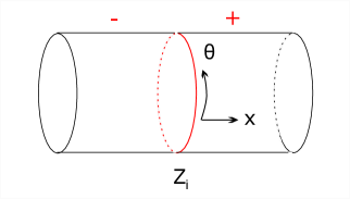
Figure 1. Preferred local coordinates around $Z_{i}$

Consider now for a moment $S$, a compact oriented surface with, say, $k$ boundary circles $\{Z_{0},\dots,Z_{k-1}\}$ – think of $S$ as the closure of one of the connected components of $M\setminus Z$ – equipped with a volume form $\omega_{0}$. What are possible orientations on the boundary circles that can be induced by a log Poisson structure $\pi$ whose vanishing circles are precisely the $Z_{i}$?

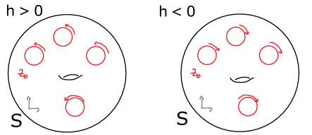
Figure 2. With a chosen global orientation of $S$, the sign of the function $h$ determines the orientation of $all$ boundary circles. Here we illustrate the two possible configurations.

Proposition 2.7.

If we look at $(S,\partial S=Z=\sqcup_{i=0}^{k}Z_{i})$ with right-handed orientation given by $\omega_{0}$, any log symplectic structure with vanishing locus $Z$ will have the property that its modular vector field orients the boundary circles in the mathematically positive sense if the orientation of $\pi=h\omega_{0}^{-1}$ with $h>0$, and in the mathematically negative sense if $h<0$.

Proof.

Assume that $h>0$; if it is not, flip the global orientation by changing the sign of $\omega_{0}$.

Pick two boundary circles, WLOG named $Z_{0},Z_{1}$, and a path $\gamma:[0,1]\rightarrow S$ connecting $Z_{0}$ to $Z_{1}$, i.e. $\gamma(0)\in Z_{0},\gamma(1)\in Z_{1}$, such that $\gamma(t)\in\operatorname{Int}(S)$ for all $t\neq 0,1$. Choose a tubular neighbourhood $U$ of the image of $\gamma$. This is diffeomorphic to a strip $[0,1]\times(-\varepsilon,\varepsilon)$. Also pick sets of local coordinates $(x_{0},\theta_{0})$ and $(x_{1},\theta_{1})$ as above on neighbourhoods $V_{0},V_{1}$ around both chosen circles. For simplicity, assume that $\gamma(0)$ and $\gamma(1)$ are the respective origins of these coordinates. Then equip $U$ with local coordinates $(a,b)$, which agree with $(x_{0},\theta_{0})$ on $U\cap V_{0}$, i.e.

$$x_{0}=a,\ \theta_{0}=b\text{ on }V_{0}\cap U.$$

We further require that $\omega_{0}=\operatorname{d\!}a\wedge\operatorname{d\!}b$ on all of $U$.

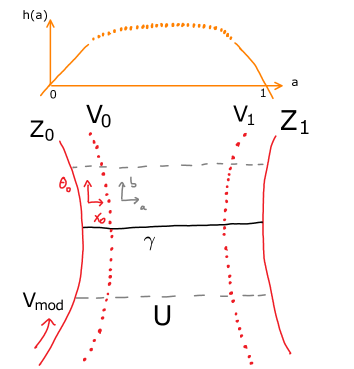
Figure 3. Illustration of the path between two boundary circles $Z_{0},Z_{1}$ of $S$ together with chosen coordinate neighbourhoods and a graph of the function $h$ near the endpoints of $\gamma$. The dotted section of the graph indicates that the precise behaviour of $h$ is unknown in this section; we only know that $h>0$.

We have started from the assumption that $\pi=h\pi_{0}$ with $h>0$ on $\operatorname{Int}(S)$. Drawing $\left(\frac{\partial}{\partial a},\frac{\partial}{\partial b}\right)$ as a right-handed coordinate basis with $\frac{\partial}{\partial b}$ pointing upwards, as in Figure 3, with the given assumptions, we must have that the modular vector field of $\pi$ restricted to $Z_{0}$ points upwards as well: The modular vector field on $Z_{0}$ is given by $c_{0}\frac{\partial}{\partial\theta_{0}}$ for a positive constant $c_{0}$, and by assumption $\frac{\partial}{\partial\theta}=\frac{\partial}{\partial b}$.

On $V_{1}$,

$$\pi=c_{1}x_{1}\frac{\partial}{\partial x_{1}}\wedge\frac{\partial}{\partial\theta_{1}}\text{ with }c_{1}>0,\ \pi_{0}=\frac{\partial}{\partial x_{1}}\wedge\frac{\partial}{\partial\theta_{1}}.$$

At the same time, $\frac{\partial h}{\partial a}|_{V_{1}}<0$, so on the overlap $U\cap V_{1}$, we must have $a\propto-x_{1}$. Since $(x_{1},\theta_{1})$ are by definition also right-handed coordinates, $\frac{\partial}{\partial x_{1}}$ points to the left in our picture Figure 3 and $\frac{\partial}{\partial\theta_{1}}$ points downwards, i.e. the modular vector field does, too.

Repeating this process for all boundary circles of $S$ (since $S$ is connected, we can draw paths between $Z_{0}$ and all other boundary circles, and we can choose these s.t. they are all distinct), this means that when looking at $S$ with the chosen global orientation being right-handed, all boundary circles are oriented in the mathematically positive sense if $h>0$ in the interior of $S$, and correspondingly, that all boundary circles are oriented in the mathematically negative sense if $h<0$. (See Figure 2 for an illustration.) ∎

For any log symplectic structure, the orientation of all vanishing circles is consequently determined by the overall sign of the bivector $\pi$ – if we change $\pi$ to $-\pi$, the orientation of all vanishing circles changes, too. Thus, for a given oriented surface $(M,\omega_{0})$ with configuration of circles $\{Z_{i}\}$, the orientation information of a log symplectic structure with vanishing circles $Z_{i}$ precisely corresponds to the choice of a 2-colouring of the corresponding bipartite graph.

We can now formulate Radko’s classification result more precisely:

Theorem 2.8.

(Classification, graph formulation) On a given connected oriented closed surface (with a fixed choice of orientation) $(M,\omega_{0})$ of genus $g$, the log symplectic structures $\pi$ are, up to orientation-preserving Poisson isomorphism, in one-to-one correspondence with graphs with the following properties and decorations:

1. The graph $\Gamma$ is equipped with a 2-colouring. (I.e. it is a bipartite graph.) Additionally, each vertex is decorated with a natural number $g_{j}\in\mathbb{N}_{0}$, satisfying $\sum_{j}g_{j}+\operatorname{genus}(\Gamma)=g$.

2. Each edge is labelled with a positive real number $\tau_{i}$, the modular period of the corresponding vanishing circle.

3. The entire graph is assigned a real number $V(\pi)$, the regularised Liouville volume.

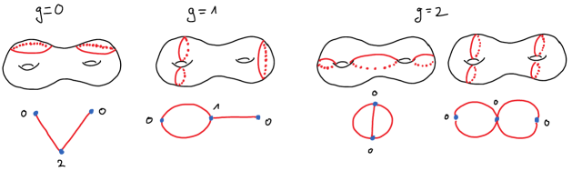
Figure 4. Examples of possible zero loci of log symplectic structures on the orientable surface of genus two, together with the corresponding bipartite graphs. Here, $g$ denotes the genus of the graph.

Example 2.9.

The sphere $M=S^{2}$. As noted in [Rad02], the log symplectic structures on the sphere can be described in terms of trees, i.e. bipartite graphs of genus zero, equipped with a vertex 2-colouring and positive real labels on each edge. There are many log symplectic structures of interest on $S^{2}$, of increasing complexity, but when we simply say the log symplectic sphere or the standard log symplectic sphere, we mean the log symplectic structure associated to the following decorated graph:

This is the log symplectic structure with a single vanishing circle along the equator and modular period $\tau=2\pi$ (thus $c=1$). If the vanishing cycle is on the equator, the contributions of the two hemispheres to the regularised Liouville volume precisely cancel, so $V(\pi)=0$.

Moving the vanishing circle away from the equator, enlarging either the positive or the negative hemisphere, leaves the graph itself invariant, but changes the overall volume to a positive or negative number.

Adding additional vanishing circles at other level sets of the height function (assuming $S^{2}$ to be embedded in $\mathbb{R}^{3}$ with the standard embedding) gives us the necklace Poisson structures. Their graphs are trees without any branches.

2.3. Compact Lagrangians and Hamiltonian isotopies

The ultimate goal of this project is to extend the concept of Fukaya category to the setting of log symplectic geometry; meaning in the simplest case to compact oriented log symplectic surfaces. The objects of the Fukaya category of a symplectic manifold are (certain classes of) Lagrangians (potentially equipped with additional data). Log symplectic structures are genuinely symplectic on a dense subset of the manifold. For our purposes in this article the following naive definition for Lagrangians not entirely contained in the degeneracy locus $Z$ is sufficient:

Definition 2.10.

A Lagrangian submanifold in a log symplectic manifold $(M,Z)$ is a submanifold which is Lagrangian outside $Z$.

We are interested in compact embedded oriented Lagrangians which intersect the degeneracy locus $Z$ transversely. Such Lagrangians have been studied in general dimensions by multiple authors, including in [KL18, GZ22].

(Potential other objects of the Fukaya category – those that lie entirely inside $Z$ – will be discussed in future work. As it turns out, the Floer differential of any intersection point in $Z$ is trivial, and the same holds true for higher $A_{\infty}$-operations.)

In 2 dimensions, the Lagrangian condition is of course trivial, so our object of interest inside closed surfaces are embedded oriented circles intersecting $Z$ transversely, in a finite set of points. Any Lagrangians that do not intersect $Z$ at all are fully covered by the symplectic theory, so we are going to focus on the case where this intersection is actually non-empty. We are also going to consider oriented log symplectic surfaces with boundary, where the vanishing locus of the log Poisson bivector is precisely the boundary – these are the objects obtained when a closed oriented log symplectic surface is cut apart along all of its vanishing circles. The relevant connected Lagrangians in this setting are embedded closed intervals which intersect the boundary transversely in their endpoints, but which do not intersect it otherwise. (Note that a single circular Lagrangian in a closed log symplectic surface can be separated into several disjoint intervals when the surface is cut apart into components, but in that setting we are still going to identify each connected component as a separate Lagrangian.)

The notion of Hamiltonian vector field and Hamiltonian isotopy exists for any Poisson structure, and so in particular for any log symplectic structure:The Hamiltonian vector field $X_{f}$ associated to a smooth function $f\in C^{\infty}(M)$ is $X_{f}=\pi(\operatorname{d\!}f)$. A Hamiltonian isotopy is the isotopy obtained as the flow of a (potentially time-dependent) Hamiltonian vector field.

Considering again a log symplectic surface $(M^{2},Z)$: Recall that in a neighbourhood of each vanishing circle $Z_{i}$, the log symplectic structure $\pi$ can be written as

$$\pi=c_{i}x\frac{\partial}{\partial x}\wedge\frac{\partial}{\partial\theta}.$$

In these coordinates, the Hamiltonian vector field of $f$ is given by:

(2) $$X_{f}=\pi(\operatorname{d\!}f)=c_{i}x\frac{\partial f}{\partial x}\frac{\partial}{\partial\theta}-c_{i}x\frac{\partial f}{\partial\theta}\frac{\partial}{\partial x}$$

Like $\pi$, this of course vanishes linearly on $Z$, and consequently every Hamiltonian isotopy restricts to the identity on $Z$: This means in particular that no two Lagrangians which intersect $Z$ in a different set of points can be Hamiltonian isotopic. Furthermore, any Lagrangian intersecting $Z$ in at least two points (when considering compact embedded circles in a closed surface, this means all Lagrangians that intersect $Z$ at all) is non-contractible under Hamiltonian isotopy.

Here we can already see some important differences to the purely symplectic case: Lagrangians that intersect $Z$ in different points cannot be related by Hamiltonian isotopy, so log symplectic surfaces have many more equivalence classes of Lagrangians up to Hamiltonian isotopy than symplectic surfaces of the same genus; more Lagrangians need to be considered genuinely different.

Furthermore, the fact that no compact Lagrangian that intersects $Z$ in at least two points (i.e. whenever an embedded compact Lagrangian intersects $Z$ at all), are contractible under any isotopy fixing $Z$ will turn out to ensure that disc bubbling – an obstruction to the Floer differential squaring to zero – cannot arise.

3. Log Floer cohomology for log symplectic surfaces

In this section, we mainly follow the exposition of combinatorial Floer cohomology for surfaces in [dSRS14], which we extend and adapt to the log symplectic setting. We will also make use of the in many ways complementary exposition in [Abo08].

Like before, let $(M,Z)$ denote a closed oriented surface (with fixed orientation form $\omega_{0}$) equipped with log Poisson structure $\pi$ whose vanishing locus is $Z$, and $S$ an oriented surface with $k$ boundary circles $Z=\{Z_{0},\dots,Z_{k-1}\}$, to be understood as the closure of one of the symplectic components of $M$.

As briefly mentioned above, here we focus on Lagrangians whose intersection with $Z$ is non-empty: As soon as one of the compact Lagrangians lies entirely inside a single symplectic component of $M$, the known results on Floer theory for symplectic surfaces apply.

As in the purely symplectic case, Lagrangian intersection Floer cohomology for log symplectic surfaces is combinatorial, but we include a discussion of the notion of pseudoholomorphic strips and the Cauchy-Riemann equation in the log symplectic setting.

3.1. Surface with boundary and a single symplectic component

WLOG assume that the orientations defined by $\omega_{0}$ and the log symplectic form $\omega=\pi^{-1}$ on $S$ agree, i.e. the sign of the function $h$ s.t. $\pi=h\pi_{0}$ is positive on the interior of $S$. (The case where the two orientations disagree on a symplectic component only becomes important when there is more than one.)

Let $(\alpha,\partial\alpha),(\beta,\partial\beta)\subset(S,Z)$ be two compact connected oriented embedded Lagrangians with boundary, i.e. oriented embedded intervals beginning and ending in some boundary component of $S$, which intersect $Z$ transversely. To begin with, assume that

(3) $$\alpha\cap\beta\cap Z=\emptyset.$$

(This implies in particular that $\alpha,\beta$ are non-isotopic under smooth isotopies which are trivial on the boundary.)

From now on, when referring to smooth isotopy on a log symplectic surface, we always mean those isotopies that restrict to the identity on the vanishing locus.

o X[c]X[c]
Case 0: $\deg(p)=0$	Case 1: $\deg(p)=1$

Figure 5. Degrees of intersection points of Lagrangians when $h>0$.

Definition 3.1.

The Floer cochain group from $\alpha$ to $\beta$ over $\mathbb{Z}_{2}$ is

(4) $$CF(\alpha,\beta):=\bigoplus_{p\in\alpha\cap\beta}\mathbb{Z}_{2}p.$$

Each intersection point $p\in\alpha\cap\beta$ can be assigned a degree in $\mathbb{Z}_{2}$:

(5) $$\deg(p):=\left\{\begin{matrix}0&\text{if a neighbourhood of }p\text{ looks like in Figure \ref{fig:deg+}, Case 0},\\ 1&\text{if a neighbourhood of }p\text{ looks like in Figure \ref{fig:deg+}, Case 1}.\end{matrix}\right.$$

This makes $CF(\alpha,\beta)$ into a graded $\mathbb{Z}_{2}$-vector space: $CF(\alpha,\beta)=CF^{0}(\alpha,\beta)\oplus CF^{1}(\alpha,\beta)$.

Remark 3.2.

1. For simplicity, we will restrict the discussion to Floer theory over $\mathbb{Z}_{2}$ in this paper; it is possible to work over $\mathbb{Z}$ instead.

2. The degree of an intersection point $p$ of course depends on whether $p$ is an element of $CF(\alpha,\beta)$ or $CF(\beta,\alpha)$.

3. Note that since we have assumed $\alpha\cap\beta\cap Z=\emptyset$ (3), all intersection points lie in the interior of $S$. Taking into account the boundary $Z=\partial S$ merely means that the Lagrangians are compact with fixed endpoints under isotopy – recall that Hamiltonian isotopies of log symplectic surfaces are always trivial on the degeneracy locus $Z$.

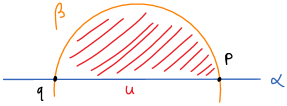
Figure 6. A smooth lune from $p$ to $q$ as elements of $CF(\alpha,\beta)$.

Definition 3.3.

(See Definition 6.1 in [dSRS14].) We call the intersection of the closed unit circle and closed upper half plane $\{z\in\mathbb{C}|\lvert z\rvert\leq 1,\operatorname{Im}(z)\geq 0\}$ in $\mathbb{C}$ the standard lune and denote it by $\mathbb{D}$.

If $p,q\in CF(\alpha,\beta)$, a smooth lune from $p$ to $q$ is an equivalence class (up to reparametrisation) of smooth orientation-preserving immersions $u:\mathbb{D}\rightarrow\operatorname{Int}(S)$ satisfying

$$u(\mathbb{D}\cap\mathbb{R})\subset\alpha,\ u(\{\lvert z\rvert=1\})\subset\beta$$

$$u(1)=p,\ u(-1)=q$$

and s.t. the corners $p,q$ of the image of $u$ are convex.

Note that smooth lunes always go between intersection points of different degree.

Definition 3.4.

In this setting, we define the Floer differential as follows:

(6) $$\partial:CF(\alpha,\beta)\rightarrow CF(\alpha,\beta),\ \partial(p)=\sum_{q\in\alpha\cap\beta}n(p,q)q,$$

where $n(p,q)\in\mathbb{Z}_{2}$ is the number of smooth lunes from $p$ to $q$ modulo 2.

The pair $(CF(\alpha,\beta),\partial)$ is then the Floer cochain complex or simply Floer complex from $\alpha$ to $\beta$.

Theorem 3.5.

(c.f. Theorems 9.1, 9.2 in [dSRS14].) For non-isotopic $(\alpha,\partial\alpha),(\beta,\partial\beta)$, the map $\partial$ does indeed make $CF(\alpha,\beta)$ into a differential complex, i.e. $\partial\circ\partial=0$. Furthermore, the associated Floer cohomology

(7) $$HF(\alpha,\beta):=\ker(\partial)/\operatorname{Im}(\partial)$$

is invariant under isotopies of $S$ which fix $Z$, i.e.

$$HF(\alpha^{\prime},\beta)=HF(\alpha,\beta),$$

where $\alpha^{\prime}$ and $\alpha$ are related by an isotopy that keeps their endpoints fixed.

Proof.

In this particular case, the symplectic argument as outlined in [dSRS14] directly translates in its entirety: $Z$, the boundary and vanishing locus of $\pi$, does not play any role. ∎

Remark 3.6.

Theorem 3.5 immediately extends to Lagrangians $\alpha=\sqcup_{i}\alpha_{i}$ with multiple connected components $\alpha_{i}$, where each $\alpha_{i}$ is an embedded interval with endpoints in $Z$ and $\alpha_{i}\cap\alpha_{j}=\emptyset$ for $i\neq j$.

Next, consider the case where the two Lagrangians $\alpha$ and $\beta$ share at least one intersection point with $Z$, i.e.

$$\alpha\cap\beta\cap Z\neq\emptyset.$$

In this case, issues specific to log symplectic geometry do arise: Should smooth lunes with endpoints in $Z$ be included into the definition of the Floer differential? Furthermore, irrespective of whether such lunes are included or not, the naive definition of the Floer complex as above will no longer yield a cohomology that is invariant under isotopy with fixed endpoints:

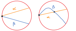
Figure 7. As soon as $\alpha\cap\beta\cap Z\neq\emptyset$, the Floer complex as naively defined above does no longer result in Floer cohomology that is invariant under isotopy with fixed endpoints.

Example 3.7.

Consider $S=D^{2}$ with log boundary $Z=\partial D^{2}$. Consider the configurations of Lagrangians $\alpha,\beta$ as in Figure 7, which are related by isotopy with fixed endpoints. On the left, there is only one intersection point, the one inside $Z$, which we call $q$. The Floer differential is trivial, so $HF(\alpha,\beta)=\mathbb{Z}_{2}$. On the right, there is an additional intersection point in the interior of $S$, which we denote by $p$. If we define the Floer differential including only lunes which do not touch $Z$, it is again zero, so $HF(\alpha,\beta)=(\mathbb{Z}_{2})^{2}$. If we do include such lunes, $\partial p=q,\partial q=0$, i.e. $\ker\partial=\operatorname{Im}\partial$, so $HF(\alpha,\beta)=0$.

In order to fix this, for any $\alpha,\beta$ we set $CF(\alpha,\beta)\equiv CF(\alpha,\phi^{t}_{H}(\beta))$, where $\phi^{t}_{H}$ is the flow of the Hamiltonian vector field $X_{H}$ of the function $H\in C^{\infty}_{+}(S,Z)$. By $C^{\infty}_{+}(M,Z)$ we mean the subset of smooth functions on $M$ that are of the form

(8) $$H(x,\theta)=f(x,\theta)\cdot x,\text{ where }f>0,$$

on a tubular neighbourhood of $Z$ with coordinates $(x,\theta)$ as above.

Definition 3.8.

We call functions in $C^{\infty}_{+}(S,Z)$, i.e. of local form given in equation 8, admissible Hamiltonians.

We require the time $t$ to be sufficiently large, so that further perturbation (i.e. bigger $t$) no longer changes the topological arrangement of $\alpha,\beta$ near $Z$. The Hamiltonian isotopy associated to an admissible Hamiltonian will always perturb a Lagrangian in the direction of the modular vector field of $\pi$ on $Z$ near $Z$. This is illustrated in Figure 8.

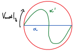
Figure 8. A Lagrangian $\alpha$ is perturbed with an admissible Hamiltonian isotopy to $\alpha^{\prime}=\phi_{H}^{1}(\alpha)$.

If $\alpha\cap\beta\cap Z=\emptyset$, this modification of the definition of Floer complex to include perturbation by an admissible Hamiltonian changes nothing (the original definition already resulted in all isotopies with fixed endpoints inducing quasi-isomorphisms). Returning to Example 3.7, we can now see that $CF(\alpha,\beta)\neq CF(\beta,\alpha)$, but that each corresponding cohomology (whether including the discs reaching $Z$ or not) is invariant under admissible Hamiltonian isotopy. The two configurations in Figure 7 now correspond to two different cochain complexes.

o X[c]X[c]
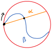
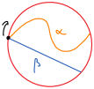
$CF(\alpha,\beta)$	$CF(\beta,\alpha)$

Figure 9. The Floer complexes associated to two Lagrangians in the log symplectic disc with one common intersection point in $Z$.

This behaviour is nothing new: Various notions of Lagrangian Floer cohomology in non-compact symplectic manifolds perturb Lagrangians going off to infinity using Hamiltonians with specific behaviour near $\infty$. This similarly results non-symmetric Floer complexes and cohomology. Of course $S\setminus Z$ is a non-compact symplectic manifold, and Lagrangians that intersect $Z$ go off to infinity in $S\setminus Z$. In this setting of a symplectic surface with log boundary, this is a form of infinitesimally wrapped Floer cohomology.

Note that we can now also unambiguously define the Floer complex of a single Lagrangian in $(S,Z)$:

(9) $$CF(\alpha):=CF(\alpha,\alpha^{\prime}),$$

where $\alpha^{\prime}$ is the image of $\alpha$ under an admissible Hamiltonian isotopy, for example like in Figure 8.

Definition 3.9.

The log Floer differential is the map

(10) $$\partial:CF(\alpha,\phi_{H}(\beta))\rightarrow CF(\alpha,\phi^{t}_{H}(\beta)),\partial(p)=\sum_{q\in\alpha\cap\phi_{H}(\beta)}n_{\operatorname{int}}(p,q)q,$$

where $n_{\operatorname{int}}(p,q)\in\mathbb{Z}_{2}$ is the number of smooth lunes which lie entirely in $\operatorname{Int}(S)$ from $p$ to $q$ modulo 2 and $\phi_{H}$ a Hamiltonian isotopy associated to $H\in C^{\infty}_{+}(S,Z)$, $H=f\cdot x$ with $f$ sufficiently large near $Z$ (in the sense defined above). Log Floer cohomology is the resulting cohomology $HF(\alpha,\beta)=\ker(\partial)/\operatorname{Im}(\partial)$.

Remark 3.10.

In the following, we will simply write $CF(\alpha,\beta)$ for this complex; the modification of the second Lagrangian by an admissible Hamiltonian isotopy is implied. Furthermore, we will simply say ‘Floer complex, Floer differential’ and ‘Floer cohomology’ when we mean the log versions defined here. If we want to include lunes with endpoints inside $Z$, we will explicitly point this out.

Above, we have already assigned a degree to intersection points of $\alpha$ and $\beta$ in the interior of $S$. With the above definition, points in $\alpha\cap\beta\cap Z$ always lie in the kernel of $\partial$. We assign all such points the degree $1$, a decision we will further motivate below.

Theorem 3.11.

For two oriented connected Lagrangians $(\alpha,\partial\alpha),(\beta,\partial\beta)$ in the log symplectic surface $(S,Z)$ which intersect $Z$ transversely and precisely in their boundaries, the map $\partial$ as in Definition 3.9 makes $CF(\alpha,\beta)$ into a differential complex, i.e. $\partial\circ\partial=0$. Furthermore, the associated log Floer cohomology is invariant under Hamiltonian isotopy associated to admissible Hamiltonians $H\in C^{\infty}_{+}(S,Z)$.

Proof.

If $\alpha\cap\beta\cap Z=\emptyset$, this reduces to Theorem 3.5, so assume that $\alpha$ and $\beta$ intersect in at least one of their two endpoints, which lie inside $Z$. Let $p$ be such a point. According to the definition of $CF(\alpha,\beta)$, perturb $\beta$ using $\phi_{H},H\in C^{\infty}_{+}(M,Z)$ so that $\alpha\pitchfork\beta$. Then a neighbourhood of $p$ looks looks like in Figure 10.

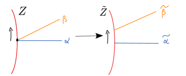
Figure 10. On the left: A neighbourhood of $p\in\alpha\cap\beta\cap Z$ when considering $p\in CF(\alpha,\beta)$. On the right, we have performed a real oriented blow-up of $p$, resulting in $\tilde{\alpha},\tilde{\beta}$, the lifts of the original Lagrangians, intersecting $\tilde{Z}$ in different points.

We now perform a real oriented blow-up of $p$, replacing $p$ by an interval (or circle segment). The resulting surface is still log symplectic ($\omega$ pulls back to a log symplectic form) and $\alpha,\beta$ lift to Lagrangians intersecting the new boundary $\tilde{Z}$ transversely (Furthermore, a real oriented blow-up of a boundary point does not change the topology of $(S,Z)$). However, since $\alpha,\beta$ originally intersected $Z$ in different angles, after blow-up, they intersect $\tilde{Z}$ in different points.
Of course, $\alpha,\beta\subset S$ are entirely unchanged after the blow-up apart from this, and the log Floer complex $CF(\tilde{\alpha},\tilde{\beta})$ is the same as the original $CF(\alpha,\beta)$. But $\tilde{\alpha},\tilde{\beta}$ satisfy the condition for Theorem 3.5, which we can now apply. In this context only $H\in C^{\infty}_{+}(S,Z)$ (instead of any Hamiltonian) are allowed – this is because more general Hamiltonians would be able to switch the position of $\alpha$ and $\beta$ near $p$, resulting in topologically distinct situations after blow-up. ∎

Proposition 3.12.

For $(\alpha,\partial\alpha)\subset(S,Z)$ an embedded interval which transversely intersects $Z$ only in its endpoints, we have

$$HF^{0}(\alpha,\alpha) \cong\mathbb{Z}_{2}$$

$$HF^{1}(\alpha,\alpha) \cong(\mathbb{Z}_{2})^{2}$$

, while the log de Rham cohomology of $\alpha$ with respect to its endpoints $Z\cap\alpha$ is

$$H^{0}(\alpha,\log\alpha\cap Z)\cong\mathbb{R},\ H^{1}(\alpha,\log\alpha\cap Z)\cong\mathbb{R}^{2}$$

This means that the log Floer cohomology of a single interval $\alpha$ reduces to the log cohomology of $\alpha$ relative to its intersection with $Z$.

Proof.

According to the Mazzeo-Melrose theorem (Proposition 2.49 in [Mel93]), the log cohomology of a manifold with smooth hypersurface $(M,N)$ is

(11) $$H^{k}(M,\log N)\cong H^{k-1}(N)\oplus H^{k}(M),$$

so for the embedded interval we do indeed obtain:

$$H^{0}(\alpha,\log Z\cap\alpha) =H^{0}(\alpha)\cong\mathbb{R}_{2}$$

$$H^{1}(\alpha,\log Z\cap\alpha) =H^{0}(Z\cap\alpha)\oplus H^{1}(\alpha)\cong\mathbb{R}^{2}$$

By the Weinstein Lagrangian neighbourhood theorem for Lagrangians in log symplectic manifolds (see Theorem 5.18 in [KL18]), we can take a tubular neighbourhood of $(\alpha,\alpha\cap Z)$ in $(S,Z)$ that is symplectomorphic to a neighbourhood of the zero section in the log cotangent bundle $T^{*}\alpha(\log\alpha\cap Z)$. Lagrangians near $\alpha$ that are Hamiltonian isotopic to $\alpha$ are precisely those that are graphs of exact log one-forms on $\alpha$. If $x\in[0,1]$ is a coordinate for $\alpha$, the pullback of $H(x)=-(x-\frac{1}{2})^{2}+1/4$ is an admissible Hamiltonian.

$$\operatorname{d\!}H =-2\left(x-\frac{1}{2}\right)\operatorname{d\!}x$$

$$\stackrel{{\scriptstyle\text{near }x=0}}{{=}}(-2x^{2}+x)\frac{\operatorname{d\!}x}{x}$$

$$\stackrel{{\scriptstyle\text{near }x^{\prime}:=1-x=0}}{{=}}(-2(x^{\prime})^{2}+x^{\prime})\frac{\operatorname{d\!}x^{\prime}}{x^{\prime}}$$

(We chose the admissible Hamiltonian $H$ s.t. the graph of $\operatorname{d\!}H$ in $T^{*}\alpha(\log\alpha\cap Z)$ is symmetric around the centre of the interval, $x=\frac{1}{2}$.) Clearly, $\operatorname{graph}(\operatorname{d\!}H)\subset T^{*}\alpha(\log\alpha\cap Z)$ intersects the zero section transversely in $x=0,\frac{1}{2},1$. Since there is only one intersection point in the interior of $S$, there are no smooth lunes. Thus

$$HF^{0}(\alpha) \cong\mathbb{Z}_{2}\text{ (Spanned by the interior intersection point.)}$$

$$HF^{1}(\alpha) \cong(\mathbb{Z}_{2})^{2}\text{ (Spanned by the intersection points at the ends.)}$$

∎

This is the motivation for considering a version of Floer cohomology that does not include smooth lunes starting or ending in $Z$ (although we will include lunes passing through $Z$ in the next section): For a single Lagrangian, this log Floer cohomology reduces to log de Rham cohomology.

3.2. Closed surface with multiple symplectic components

In this section we consider a closed log symplectic surface $(M,\pi,Z)$ with non-empty $Z$, i.e. at least 2 symplectic components. Again, fix an orientation $\omega_{0}$.

In the previous subsection, we described the log Floer complex and its cohomology for a symplectic component with positive sign. On those components with negative sign, we have the following changes:

o X[c]X[c]
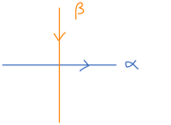
Case 0: $\deg(p)=0$	Case 1: $\deg(p)=1$

Figure 11. Degrees of intersection points of Lagrangians when $h<0$.

Definition 3.13.

(On symplectic components with negative sign) An intersection point in a component of $M\setminus Z$, $p\in CF(\alpha,\beta)$, where $h<0$ is assigned the $\mathbb{Z}_{2}$-degree

(12) $$\deg(p):=\left\{\begin{matrix}0&\text{if a neighbourhood of }p\text{ looks like in Figure \ref{fig:deg-}, Case 0},\\ 1&\text{if a neighbourhood of }p\text{ looks like in Figure \ref{fig:deg-}, Case 1}.\end{matrix}\right.$$

For two intersection points $p,q\in CF(\alpha,\beta)$ in a symplectic component with $h<0$, a smooth lune from $p$ to $q$ is an equivalence class (up to reparametrisation) of smooth orientation-reversing immersions $u:\mathbb{D}\rightarrow\operatorname{Int}(S)$ satisfying

$$u(\mathbb{D}\cap\mathbb{R})\subset\alpha,\ u(\{\lvert z\rvert=1\})\subset\beta$$

$$u(1)=p,\ u(-1)=q$$

and s.t. the corners $p,q$ of the image of $u$ are convex. (See Figure 12 for an illustration.)

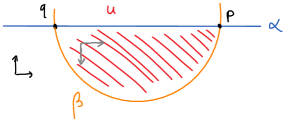
Figure 12. A smooth lune from $p$ to $q$ in $CF(\alpha,\beta)$ in a symplectic component where $h<0$. The pairs of basis vectors indicate the orientations of $\mathbb{D}$ (the standard orientation of $\mathbb{C}$, grey) and the ambient surface (as given by $\omega_{0}$, black).

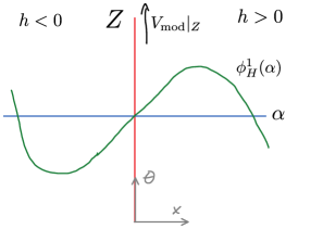
Figure 13. Perturbation of a Lagrangian $\alpha$ by an admissible Lagrangian as it crosses $Z$

Note that we still define $CF(\alpha,\beta)$ to include the sufficiently large perturbation of $\beta$ by an admissible Hamiltonian $H\in C^{\infty}_{+}(M,Z)$. Figure 13 illustrates how this looks near an an intersection of a Lagrangian with an interior component of $Z$ (which is of course bordered by symplectic components with different signs of $h$).

In addition to these lunes between pairs of intersection points lying in the interior of the same symplectic component, we now also define lunes between intersection points that lie in the interiors of different symplectic components. Such lunes only arise in $CF(\alpha,\beta)$ if $\alpha\cap\beta\cap Z\neq\emptyset$. We call such lunes crossing lunes.

Denote by $\mathbb{D}_{k}:=(\mathbb{D},I_{1}\sqcup\dots\sqcup I_{k})$ the standard lune with $k\in\mathbb{N}_{0}$ marked embedded intervals; each $I_{j}$ is an interval from $\mathbb{D}\cap\mathbb{R}$ to $\mathbb{D}\cap\{\lvert z\rvert=s^{2}+t^{2}=1\}$ with $s=\text{const}$. For any pair $(M,Z)$ of a manifold with embedded hypersurface, denote by $\mathcal{E}_{Z}$ the restriction of any Euler-like log vector field to the hypersurface $Z$: If $Z$ is given by the vanishing of a coordinate $x$, on any tubular neighbourhood we have have vector field $x\frac{\partial}{\partial x}$, which is a nowhere-vanishing section of the log tangent bundle. For the purpose of the definition, pick such an Euler-like vector field both for $(\mathbb{D},\sqcup_{j}I_{j})$ and $(M,Z)$.

Definition 3.14.

For two intersection points $p,q\in CF(\alpha,\beta)$ lying in $M\setminus Z$, a crossing lune from $p$ to $q$ is an equivalence class up to reparametrisation of smooth maps $u:\mathbb{D}_{k}\rightarrow\operatorname{Int}(S)$ (for some $k$) satisfying

$$u(\mathbb{D}\cap\mathbb{R})\subset\alpha,\ u(\{\lvert z\rvert=1\})\subset\beta$$

$$u(1)=p,\ u(-1)=q$$

and

• $u$ is orientation-preserving wherever $h>0$, and orientation-reversing wherever $h<0$ (this is to say $u$ is orientation-preserving with respect to the orientation of $M\setminus Z$ given by $\omega=\pi^{-1}$),

• $(\operatorname{Im}(u)\cap Z)\subset(\alpha\cap\beta\cap Z)$,

• For each $q\in\alpha\cap\beta\cap Z$ that lies in the Image of $u$, $u^{-1}(q)=I_{j}$ for some $j\in\{1,\dots,k\}$,

• $u$ is an immersion on $\mathbb{D}\setminus u^{-1}(Z)$, and as a map $u_{*}:T\mathbb{D}_{k}(-\log\sqcup_{j}I_{j})\rightarrow TM(-\log Z)$,

  $$u_{*}(\mathcal{E}_{\sqcup_{j}I_{j}})=\mathcal{E}_{Z},$$

• and the corners $p,q$ are convex.

We refer to $\operatorname{Im}(u)\cap Z$ as the crossings of $u$.

Since $u$ is orientation-preserving ($\det(u_{*})>0$) on positive symplectic components and orientation-reversing ($\det(u_{*})<0$) on negative ones, $\det{u_{*}|_{Z}}=0$, so $u$ cannot be an immersion on all of $\mathbb{D}$ if it is to pass through $Z$.

Remark 3.15.

1. Clearly, the above definition reduces to those we have previously given for smooth lunes if $u^{-1}(Z)=\emptyset$. When we talk about the set of crossing lunes or number of crossing lunes between two points, we usually mean all lunes, including those that do not actually pass through $Z$. When we talk about a specific crossing lune, it will be one where $\operatorname{Im}(u)\cap Z$ is non-trivial, otherwise we will refer to it as a smooth lune.

2. In fact, with our definition of admissible Lagrangians and $CF(\alpha,\beta)$, crossing lunes will only ever have one crossing: Assume that we have a crossing lune passing through both $q_{1},q_{2}\in\alpha\cap\beta\cap Z$. Consider the submanifold of $M$ enclosed by $\alpha,\beta$ between $q_{1},q_{2}$. This is diffeomorphic to a disc whose boundary is the union of two arc segments $\bar{\alpha}\subset\alpha$ and $\bar{\beta}\subset\beta$. Consequently, $\bar{\alpha}$ and $\bar{\beta}$ are isotopic with fixed endpoints. But this is a contradiction: If the segments $\bar{\alpha},\bar{\beta}$ are isotopic with fixed endpoints in $Z$ and we are considering $CF(\alpha,\beta)\equiv CF(\alpha,\phi_{H}(\beta))$, we have already perturbed $\beta$ sufficiently far with an admissible Hamiltonian, which will always result in at least one intersection point of $\alpha,\beta$ in the interior of every symplectic component that a crossing lune through either $q_{1}$ or $q_{2}$ would begin or end at.
   Consequently, we will take the domain of each crossing lune to be $(\mathbb{D},I_{1}=\{s=0\})$.

Definition 3.16.

Given two non-contractible Lagrangians $\alpha,\beta$ in a closed oriented log symplectic surface $(M,\pi,Z)$, the log Floer differential is the map

(13) $$\partial:CF(\alpha,\beta)\equiv CF(\alpha,\phi^{t}_{H}(\beta))\rightarrow CF(\alpha,\beta),\ \partial(p)=\sum_{q\in\alpha\cap\phi_{H}(\beta)}n_{c}(p,q)q,$$

where $\phi^{t}_{H}$ is a sufficiently large Hamiltonian isotopy associated to $H\in C^{\infty}_{+}(S,Z)$ and $n_{c}(p,q)$ is the number of crossing lunes from $p$ to $q$ mod 2. (In particular, $n_{c}(p,q)=0$ if either $p$ or $q$ lies in $Z$.)

Theorem 3.17.

Let $\alpha,\beta\subset(M,Z)$ be two embedded compact Lagrangians in the closed oriented log symplectic surface $(M,Z)$ that intersect $Z$ transversely and non-trivially. Then the map $\partial$ as in Definition 3.16 makes $CF(\alpha,\beta)\equiv CF(\alpha,\phi_{H}(\beta)$ into a differential complex, i.e. $\partial\circ\partial=0$. Furthermore, the associated log Floer cohomology is invariant under Hamiltonian isotopy associated to admissible Hamiltonians $H\in C^{\infty}_{+}(M,Z)$.

Proof.

If $\alpha\cap\beta\cap Z=\emptyset$, this reduces to Theorem 3.5 in each symplectic component of $(M,Z)$, so assume that $\alpha\cap\beta\cap Z$ contains at least one point. If $p\in\alpha\cap\beta\cap Z$, $\partial(p)=0$, so $\partial^{2}(p)=0$.

In order to prove that $\partial^{2}(p)=0$ for $p\in\alpha\cap\beta\cap(M\setminus Z)$, perform the following surgery on $M$:

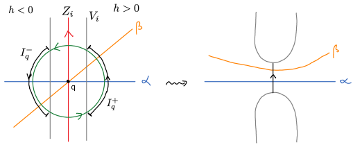
Figure 14. This is an illustration of the surgery performed around each $q\in\alpha\cap\beta\cap Z$ identifying $I^{+}_{q}$ and $I^{-}_{q}$, where on the right we have ‘untwisted’ the resulting surface. This surgery resolves the intersection point $q$, while still resulting in an orientable surface globally.

1. Choose a tubular neighbourhood $V_{i}$ for each of the connected components $Z_{i}\subset Z$ that contain a $q\in\alpha\cap\beta\cap Z$. Each $V_{i}$ has to be sufficiently small so as to contain no intersection points of $\alpha$ and $\beta$ except those in $\alpha\cap\beta\cap Z$.

2. Choose a $D^{2}$-neighbourhood $U_{q}$ centred each $q\in\alpha\cap\beta\cap Z$, sufficiently large s.t.

   $$M^{\prime}:=\left(M\setminus\left(\bigcup_{i}V_{i}\right)\right)\cup\left(\bigcup_{q\in\alpha\cap\beta\cap Z}U_{q}\right)$$

   is connected, but sufficiently small s.t. $U_{q}$ contains no intersection points of $\alpha,\beta$ other than $q$, nor other points in $(\alpha\cup\beta)\cap Z$. Equip $U_{q}$ with polar coordinates $(r_{q},\vartheta_{q})$, chosen s.t. their orientation agrees with that of $\omega$ and $r_{q}=x_{i}$. This determines the orientation of the circle $\partial U_{q}$.

3. For each $q$, denote by $I^{+}_{q},I^{-}_{q}$ the connected components of

   $$(\partial U_{q})\cap\left(M\setminus\left(\bigcup_{i}V_{i}\right)\right),$$

   where the sign of each is determined by whether $h$ is positve or negative. The $I^{\pm}_{q}$ inherit an orientation from $\partial U_{q}$.

4. Finally, set

   (14) $$\tilde{M}:=M\setminus\left(\bigcup_{i}V_{i}\cup\bigcup_{q\in\alpha\cap\beta\cap Z}U_{q}\right)/\sim_{\phi},$$

   where $\phi:\bigcup_{q}I^{+}_{q}\rightarrow\bigcup_{q}I^{-}_{q}$ is an orientation-preserving diffeomorphism that identifies each $I^{+}_{q}$ with the corresponding $I^{-}_{q}$ such that

   $$\phi(I^{+}_{q}\cap\alpha) =I^{-}_{q}\cap\alpha$$

   $$\phi(I^{+}_{q}\cap\beta) =I^{-}_{q}\cap\beta$$

   As written, $\tilde{M}$ is a surface with corners, but these can be smoothed out, as can corners that might have arisen in $\alpha$ and $\beta$.

This procedure is illustrated in Figure 14 around a single point $q\in\alpha\cap\beta\cap Z$.

Note that $\tilde{M}$ is an oriented surface: We will show this by doing the surgery on each $Z_{i}$ sequentially, building $\tilde{M}$ step by step, with an oriented surface at each step. Any $Z_{i}$ separates $M$ into two oriented parts, which we call $M_{i}^{+},M_{i}^{-}$ according to the sign of the symplectic component bordering $Z_{i}$. The boundaries $\partial M^{+}_{i},\partial M^{-}_{i}$ inherit orientations from $Z_{i}$. By the way we have defined the orientations of the $I^{\pm}_{q}$ (for $q\in Z_{i}$) we can see that the orientations of the $I^{+}_{q}$ agree with the orientation of $\partial M^{+}_{i}$, while the orientations of $I^{-}_{q}$ are the opposite of $\partial M^{-}_{i}$. So now flip the orientations of $M^{-}_{i}$ and its boundary, which also changes the sign of every symplectic component of $M^{-}_{i}$. When we now glue together the matching $I^{\pm}_{q}$ using $\phi$, both the orientations of the glued segments, as well as their normal orientations agree, resulting in a globally oriented surface. This surface is no longer closed, but can be viewed as a surface with boundary.

It can happen that the resulting $\tilde{\alpha},\tilde{\beta}\subset\tilde{M}$ are no longer circles, but instead collections of intervals ending in $\partial\tilde{M}$, but their intersection points have only changed in that all $q\in\alpha\cap\beta\cap Z$ have been removed. All lunes remain the same, with the exception that lunes with non-trivial crossings are now just smooth lunes:

(15) $$(CF(\alpha,\beta),\partial)\cong(CF(\tilde{\alpha},\tilde{\beta}),\partial)\oplus\left(\bigoplus_{q\in\alpha\cap\beta\cap Z}\mathbb{Z}_{2}q,\ 0\right)$$

We are thus again in the setting of Theorem 3.5. ∎

Remark 3.18.

This presentation of the proof does not make it explicit, but upon inspection, it becomes clear that no Lagrangian $\alpha$ intersecting $Z$ before the surgery will admit a disc bubble, i.e. a a disc bounded entirely by $\alpha$ – we have established that pseudoholomorphic discs can only hit $Z$ in discrete points. The surgery is constructed in such a way that the resulting compact Lagrangians in the open honestly symplectic surface are non-contractible; there are thus no disc bubbles either.

The result of Proposition 3.12 on the log Floer cohomology of a single closed Lagrangian carries over to this setting with multiple symplectic components:

Proposition 3.19.

For $\alpha\subset(M,Z)$ a closed embedded Lagrangian in an oriented log symplectic surface that intersects $Z$ transversely in $k$ points, we have

$$HF^{0}(\alpha,\alpha) \cong\mathbb{Z}_{2}$$

$$HF^{1}(\alpha,\alpha) \cong(\mathbb{Z}_{2})^{k}\oplus\mathbb{Z}_{2},$$

while the log de Rham cohomology of $\alpha$ with respect to its endpoints $Z\cap\alpha$ is

$$H^{0}(\alpha,\log\alpha\cap Z)\cong\mathbb{R},\ H^{1}(\alpha,\log\alpha\cap Z)\cong\mathbb{R}^{k}\oplus\mathbb{R}$$

This means that the log Floer cohomology of a single closed Lagrangian $\alpha\cong S^{1}$ again reduces to the log cohomology of $\alpha$ relative to its intersection with $Z$.

Proof.

Again using Mazzeo-Melrose’s result (11), we find

$$H^{0}(\alpha,\log\alpha\cap Z) =H^{0}(\alpha)=H^{0}(S^{1})\cong\mathbb{R}$$

$$H^{1}(\alpha,\log\alpha\cap Z) =H^{0}(Z\cap\alpha)\oplus H^{1}(\alpha)=H^{0}(\{\text{pt}\}^{\lvert\alpha\cap Z\rvert})\oplus H^{1}(S^{1})\cong\mathbb{R}^{\lvert Z\cap\alpha\rvert}\oplus\mathbb{R}$$

Again pick a tubular neighbourhood for $\alpha$ and identify it with an open neighbourhood of the zero section in $T^{*}\alpha(\log\alpha\cap Z)$. Pick a smooth function $H$ on $\alpha$ with the following properties:

1. In every tubular neighbourhood $\mathcal{U}_{i}$ of a $Z_{i}$ with coordinates $(x_{i},\theta_{i})$, $H|_{\mathcal{U}_{i}}=x_{i}$.

2. On every positive symplectic component of $M$, $H>0$; on every negative symplectic component, $H<0$.

Perturbing $\alpha$ with the corresponding Hamiltonian isotopy $\phi^{t}_{p^{*}H}$ (where $p:T^{*}\alpha(\log\alpha\cap Z)\rightarrow\alpha$ is the canonical projection) leads an $\alpha^{\prime}$ that intersects $\alpha$ in each point in $\alpha\cap Z$, as well as precisely once in every symplectic component that $\alpha,\alpha^{\prime}$ pass through. If $\lvert\alpha\cap Z\rvert=k$, this means that $CF(\alpha,\alpha^{\prime})$ is spanned by $q_{1},\dots,q_{k}\in\alpha\cap\alpha^{\prime}\cap Z$ and $p_{1},\dots,p_{k}\in(\alpha\cap\alpha^{\prime})\setminus Z$. Note that $k$ has to be even. WLOG assume that $p_{1}$ lies in a positive symplectic component, $q_{1}$ is adjacent, and the numbering proceeds in a mathematically positive sense according to the orientation of $\alpha$.

If $i\in\{1,\dots,k\}$ is even, two crossing lunes start in $p_{i}$: One to $p_{i-1}$, one to $p_{i+1}$, where we take $i\in\mathbb{Z}/k\mathbb{Z}$. If $i$ is odd, no crossing lunes start in $p_{i}$. Thus:

$$\partial q_{i} =0\ \forall i$$

$$\partial p_{i} =\begin{cases}p_{i-1}+p_{i+1}&\text{if }i\text{ is odd,}\\ 0&\text{if }i\text{ is even.}\end{cases}$$

So we find:

$$\ker(\partial) =\operatorname{span}\left\{q_{1},\dots,q_{k},p_{2},p_{4},\dots,p_{k},\sum_{j\text{ odd}}p_{j}\right\}$$

$$\operatorname{Im}(\partial) =\operatorname{span}\left\{p_{i-1}+p_{i+1}|i\text{ odd}\right\}$$

$$=\operatorname{span}\left\{p_{2}+p_{4},p_{4}+p_{6},\dots,p_{k-2}+p_{k}\right\}$$

As a result, the Floer cohomology is

$$HF(\alpha,\alpha^{\prime})\cong(\mathbb{Z}_{2})^{k+\frac{k}{2}+1}/(\mathbb{Z}_{2})^{\frac{k}{2}-1}\cong\mathbb{Z}^{k+2}\cong H^{\bullet}(\alpha,\log\alpha\cap Z).$$

In fact, we can make this isomorphism explicit by associating generators to each other in such a way that it respects degree, i.e. is an isomorphism of graded vector spaces: With the chosen numbering, $p_{i}$ with odd $i$ are actually intersection points of degree 0, $p_{i}$ with even $i$ of degree 1. (All $q_{i}$ are by definition of degree 1). We thus obtain an isomorphism that respects degree by assigning

(16) $$\left[q_{i}\right] \mapsto[\lambda_{i}]$$

$$\left[\sum_{i\text{ odd}}p_{i}\right] \mapsto[1]$$

$$[p_{2}] \mapsto[\zeta],$$

where $\lambda_{i}$ are the log oneforms locally given by $\lambda_{i}=\frac{\operatorname{d\!}x_{i}}{x_{i}}$, $1$ is the constant function and $\zeta$ is the closed nowhere vanishing one-form on the circle. ∎

The fact that this version of log Floer cohomology computes log cohomology with respect to the intersection locus with $Z$ motivates our decision not to consider lunes beginning or ending inside $Z$, even though this would also yield a well-defined theory.

3.3. A brief aside: Working over the Novikov field

So far in this section, we have always assumed that the Lagrangians under consideration intersect $Z$. Everything we have established so far remains applicable when just one of the Lagrangians does (this is in fact another case where Theorem 3.5 applies directly). However, in order for Floer cohomology for pairs of isotopic Lagrangians that do not intersect $Z$ to be defined, we need to work over the Novikov field and modify the definition of the Floer differential to include the symplectic volume of lunes – this is already the case for symplectic surfaces. Here we briefly outline the necessary modifications:

Definition 3.20.

The Novikov field $\Lambda$ over $\mathbb{Z}_{2}$ consists of elements

$$\sum_{i\in\mathbb{Z}}a_{i}T^{\lambda_{i}},$$

where $a_{i}\in\mathbb{Z}_{2}$ and zero for sufficiently negative $i$, $\lambda_{i}\in\mathbb{R}$ satisfying $\lim_{i\rightarrow\infty}\lambda_{i}=\infty$, and $T$ a formal parameter.

The Floer cochain complex over $\lambda$ is $CF(\alpha,\beta)=\bigoplus_{p\in\alpha\cap\phi_{H}(\beta)}\Lambda\cdot p$, and the log Floer differential is modified to

(17) $$\partial(p)=\sum_{\stackrel{{\scriptstyle q\in\alpha\cap\beta}}{{u\text{ crossing lune }p\rightarrow q}}}T^{\omega(u)}q,$$

where $\omega(u)=\int_{StL}u^{*}(\omega)$. Note that we are working in the Novikov field over $\mathbb{Z}_{2}$, so two crossing lunes from $p$ to $q$ with equal area will cancel.

This is only different from the purely symplectic case when we are counting lunes with non-trivial crossing. For these lunes, we need to demonstrate that $\omega(u)$ is well-defined. Furthermore, we need to ensure that the property $\partial\circ\partial=0$ and the invariance under admissible Hamiltonian isotopy are preserved when crossing lunes are involved.

Recall that the function $h\in C^{\infty}(M)$ s.t. $\pi=h\omega_{0}^{-1}$ vanishes precisely on $Z$ and does so linearly. Choose a coordinate neighbourhood near $Z_{i}$ s.t. $\omega=\frac{1}{c_{i}}\frac{\operatorname{d\!}x}{x}\wedge\operatorname{d\!}\theta$. Near $q\in\alpha\cap\beta\cap Z_{i}$, in a potentially smaller coordinate neighbourhood given by $x\in(-\epsilon,\epsilon)$, we can apply admissible Hamiltonian isotopies to $\alpha,\beta$ s.t.

$$\alpha =\{(x,0)\}$$

$$\beta =\{(x,\theta=x)\}$$

Now assume that a crossing lune passes through $q$. If we remove the tubular neighbourhood $\mathcal{U}$ with $x\in(-\epsilon,\epsilon)$ of $Z_{i}$, the area of the remaining lune with respect to $\omega$ is clearly finite, as it is the integral of a bounded 2-form over a compact set. We now compute the area of the lune $u$ in $\mathcal{U}$ with respect to $\omega$:

$$\int_{\mathcal{U}}\omega =\int_{-\epsilon}^{\epsilon}\int_{0}^{x}\frac{1}{x}\operatorname{d\!}\theta\operatorname{d\!}x$$

$$=\int_{-\epsilon}^{\epsilon}\operatorname{d\!}x$$

$$=2\epsilon$$

This shows that crossing lunes have a well-defined area with respect to $\omega$, even though $\omega$ is singular.

Admissible Hamiltonian isotopies preserve the symplectic area with respect to $\omega$ just like in the symplectic case. What remains is to modify the surgery employed in the proof of Theorem 3.17 and shown in Figure 14 in such a way that the area of crossing lunes does not change in the process: Instead of directly identifying $I_{q}^{\pm}$, we can insert a strip of the correct width, corresponding to the size of the neighbourhood $U_{q}$ we removed. Then we can apply the result for the Floer differential over the Novikov field proved in [Abo08], Lemma 2.11.

3.4. The Floer equation for log symplectic Floer theory and (pseudo-)holomorphic lunes

In this section, we motivate the definition of Lagrangian intersection Floer cohomology in terms of the pseudoholomorphic strips satisfying a log Floer equation. As a first step, we fix a nice type of compatible almost complex complex structure for the log symplectic form $\omega=\pi^{-1}$:

Definition 3.21.

(Compare Definition 4.1.1 in [Alb17].) An almost complex structure $J\in\operatorname{End}(TM(-\log Z))$ is cylindrical if in the adapted coordinate neighbourhood of $Z_{i}$ with coordinates $(x_{i},\theta_{i})$

(18) $$J\left(x_{i}\frac{\partial}{\partial x_{i}}\right)=c_{i}\frac{\partial}{\partial\theta_{i}},\ J\left(c_{i}\frac{\partial}{\partial\theta_{i}}\right)=-x_{i}\frac{\partial}{\partial x_{i}}.$$

Now consider smooth lunes $u:\mathbb{D}\rightarrow(M,Z)$, where $\mathbb{D}$ is equipped with the standard complex structure $I$ inherited from $\mathbb{C}$ ($z=s+it$ is the holomorphic coordinate):

$$I\left(\frac{\partial}{\partial s}\right)=\frac{\partial}{\partial t},\ I\left(\frac{\partial}{\partial t}\right)=-\frac{\partial}{\partial s}$$

The condition for $u$ to be (pseudo-)holomorphic is

$$J\circ u_{*}=u_{*}\circ I,$$

which, writing $u$ as $u=(u_{x},u_{\theta})$ (i.e. suppressing the index $i$), we can rewrite in coordinates as

(19) $$\frac{c}{u_{x}}\frac{\partial u_{x}}{\partial s} =\frac{\partial u_{\theta}}{\partial t}$$

$$\frac{c}{u_{x}}\frac{\partial u_{x}}{\partial t} =-\frac{\partial u_{\theta}}{\partial s}$$

or

(20) $$\begin{cases}c\frac{\partial\log u_{x}}{\partial s}=\frac{\partial u_{\theta}}{\partial t};c\frac{\partial\log u_{x}}{\partial t}=-\frac{\partial u\theta}{\partial s}&\text{for }u_{x}>0\\ c\frac{\partial\log-u_{x}}{\partial s}=\frac{\partial u_{\theta}}{\partial t};c\frac{\partial\log-u_{x}}{\partial t}=-\frac{\partial u\theta}{\partial s}&\text{for }u_{x}<0\end{cases}$$

which we recognise as the Cauchy-Riemann equations for the complex function $\mathfrak{u}_{+}:=c\log(u_{x})+iu_{\theta}$, where $u_{x}>0$ and $\mathfrak{u}_{-}:=c\log(-u_{x})+iu_{\theta}$ for $u_{x}<0$. By the standard definition of the complex logarithm,

$$\mathfrak{u}_{+}=\log\left(u_{x}^{c}e^{iu_{\theta}}\right) =:\log\left(u_{+}\right)$$

$$\mathfrak{u}_{-}=\log\left(-u_{x}^{c}e^{iu_{\theta}}\right) =:\log\left(u_{-}\right)$$

It thus makes sense to view each connected component of $\mathcal{U}\setminus Z$ (where $\mathcal{U}$ again denotes the standard tubular neighbourhood with coordinates $(x,\theta)$ of $Z$) as equipped with a complex structure equivalent to $\mathbb{C}\setminus\{0\}$ on each connected component, i.e. $z=x^{c}e^{i\theta}$ where $x>0$ and $z=-x^{c}e^{i\theta}$ where $x<0$. Alternative holomorphic coordinates for the same complex structures are

(21) $$\begin{cases}z=xe^{i/c\theta}&\text{for }x>0\\ z=-xe^{i/c\theta}&\text{for }x<0,\end{cases}$$

making $\tau_{i}=\frac{2\pi}{c_{i}}$ as the modular period of $Z_{i}$ more explicit. The maps $u_{\pm},\mathfrak{u}_{\pm}$ are holomorphic with respect to these complex structures.

Thus, viewing our original log almost complex structure $J\in\operatorname{End}(TM(-\log Z))$ as a complex structure on $\mathcal{U}\setminus Z$, we obtain something that looks like the neighbourhood of a conical singularity, as in Figure 15.

Figure 15. An illustration of the complex structure on $\mathcal{U}\setminus Z$: Each connected component looks like $\mathbb{C}\setminus\{0\}$ in terms of its complex structure; the origin of both components is removed.

In section 3.3 we demonstrated that crossing lunes have a well-defined, finite area with respect to the log symplectic form $\omega$. They can be viewed as pseudoholomorphic lunes according to (19) outside $Z$: According to the Riemann mapping theorem, the half discs without endpoints $\mathbb{D}_{-}:=\{z\in\mathbb{D}|-1<\operatorname{Re}(z)<0\}$ and $\mathbb{D}_{+}:=\{z\in\mathbb{D}|1>\operatorname{Re}(z)>0\}$ are (in a neighbourhood of $z=0$, if desired) biholomorphically equivalent to

$$\mathbb{S}_{-} :=\{s+it|s\in(-\infty,\infty),\ 0\leq t\leq e^{-s}\}$$

$$\mathbb{S}_{+} :=\{s+it|s\in(-\infty,\infty),\ 0\leq t\leq e^{s}\}$$

respectively.

Recall that we can perturb two Lagrangians $\alpha,\beta$ by admissible Hamiltonian isotopies s.t. inside $\mathcal{U}$, they are given by $\alpha=\{(x,0)\},\ \beta=\{(x,\theta=\frac{1}{c}x)\}$. Thus, when we restrict a crossing lune to each symplectic component of $\mathcal{U}\setminus Z$, we can represent the map $u$ by

$$u_{-}:\mathbb{S}_{-} \rightarrow\mathcal{U}_{-},(s,t)\mapsto e^{-s+it/c}$$

$$u_{+}:\mathbb{S}_{+} \rightarrow\mathcal{U}_{+},(s,t)\mapsto e^{s+it/c}$$

respectively, which are holomorphic in the sense of equation (21). When factoring these components through $\mathbb{D}$, we can smooth them out s.t. they extend over $s=0$ to a single smooth map $u$ with $u(s=0)=(x=0,\theta=0)$.

If we further include perturbation of one of the Lagrangians by an admissible Hamiltonian isotopy $H$ in order to ensure $\alpha\pitchfork\beta$ in the setting where this is not already true to begin with, we obtain a log Floer equation:

(22) $$u_{*}\left(\frac{\partial}{\partial s}\right)+J_{t}\left(u_{*}\left(\frac{\partial}{\partial t}\right)-X_{H}\circ u\right)=0$$

(23) $$\Leftrightarrow \begin{cases}u_{x}\frac{\partial u_{\theta}}{\partial s}+c\frac{\partial u_{x}}{\partial t}+c^{2}u_{x}\left.\frac{\partial H}{\partial\theta}\right|_{u}=0\\ c\frac{\partial u_{x}}{\partial s}-u_{x}\frac{\partial u_{\theta}}{\partial t}+u_{x}^{2}\left.\frac{\partial H}{\partial x}\right|_{u}=0\end{cases}$$

We thus find that log Floer cohomology is indeed a natural extension of ordinary Floer cohomology for symplectic surfaces, giving us an indication how how to extend it to higher dimensions.

4. Outlook

In the upcoming second article [KL23], we define higher $A_{\infty}$-operations for Lagrangians in compact oriented log symplectic surfaces and use, as well as an explicitly constructed collection of Lagrangians, to construct a Fukaya category. We will again argue that this definition constitutes the natural extension of the definition of Fukaya category for a symplectic surface to the log symplectic setting.

Next, we will attempt to apply the lessons learned from log symplectic surfaces to compact stable generalized complex 4-manifolds, which in many ways behave similarly. The additional challenge in this setting comes of course from the fact that the behaviour of pseudoholomorphic curves is much more complicated in 4 dimensions, and the theory will no longer be combinatorial. However, early results indicate that pseudoholomorphic strips between Lagrangians and their moduli spaces still behave well.

References

- [Abo08] Mohammed Abouzaid. On the Fukaya categories of higher genus surfaces. Adv. Math., 217(3):1192–1235, 2008.
- [Alb17] Davide Alboresi. Holomorphic curves in log-symplectic manifolds. DOI: https://doi.org/10.48550/arXiv.1711.10978, 2017.
- [dSRS14] Vin de Silva, Joel W. Robbin, and Dietmar A. Salamon. Combinatorial Floer homology. Mem. Amer. Math. Soc., 230(1080):v+114, 2014.
- [GMP14] Victor Guillemin, Eva Miranda, and Ana Rita Pires. Symplectic and Poisson geometry on -manifolds. Adv. Math., 264:864–896, 2014.
- [Gua03] Marco Gualtieri. Generalized complex geometry. PhD thesis, University of Oxford, 2003.
- [GZ22] Stephane Geudens and Marco Zambon. Deformations of Lagrangian submanifolds in log-symplectic manifolds. Adv. Math., 397:Paper No. 108202, 85, 2022.
- [Hit03] Nigel Hitchin. Generalized Calabi-Yau manifolds. Q. J. Math., 54(3):281–308, 2003.
- [KL18] Charlotte Kirchhoff-Lukat. Aspects of Generalized Geometry: Branes with Boundary, Blow-ups, Brackets and Bundles. PhD thesis, University of Cambridge, 2018.
- [KL23] Charlotte Kirchhoff-Lukat. The fukaya category of an orientable log symplectic surface. 2023. Upcoming work.
- [Mel93] Richard B. Melrose. The Atiyah-Patodi-Singer index theorem, volume 4 of Research Notes in Mathematics. A K Peters, Ltd., Wellesley, MA, 1993.
- [MP18] Eva Miranda and Arnau Planas. Equivariant classification of -symplectic surfaces. Regul. Chaot. Dyn., 23:355–371, 2018.
- [Rad02] Olga Radko. A classification of topologically stable Poisson structures on a compact oriented surface. J. Symplectic Geom., 1(3):523–542, 2002.