Detecting axion dark matter with chiral magnetic effects

Abstract

We show that dark matter axions or axion-like particles (ALP) induce spontaneously alternating electric currents in conductors along the external magnetic fields due to the (medium) axial anomaly, realizing the chiral magnetic effects. We propose a new experiment to measure this current to detect the dark matter axions or ALP. These induced currents are the electron medium effects, directly proportional to the axion or ALP coupling to electrons, which depends on their microscopic physics, and also suppressed by the Fermi velocity.

I Introduction

Though none of new particles beyond the standard model (BSM) have been found yet despite of tremendous experimental endeavors for decades, the axion is still one of the well-motivated new particles, currently being searched actively in the laboratory and also in the sky Choi:2020rgn . It could explain why quantum chromodynamics (QCD) preserves the time reversal symmetry or CP and also the parity P, known as the strong CP problem. Furthermore it is an excellent candidate for dark matter that constitutes roughly a quarter of our universe Chadha-Day:2021szb .

QCD allows in the Lagrangian a marginal theta term that breaks CP and P in general

$${\cal L}_{\rm QCD}\supset\frac{\theta}{16\pi^{2}}\epsilon^{\mu\nu\alpha\beta}\,{\rm Tr}\,F_{\mu\nu}F_{\alpha\beta}\,,$$ (1)

where $F=dA+A^{2}$ is the field strength two form of the gluon fields $A$. The $\theta$ parameter, being the coefficient of the Pontryagin index, has to be an angle variable with the $2\pi$ periodicity for the gauge theory to be consistent quantum mechanically. One of the viable solutions for the strong CP problem is to promote the $\theta$ angle to a dynamical field, namely the axion, $\theta=a(x)/f$, with the axion decay constant $f$, that relaxes to the CP-symmetric value.

Since the parameter $\theta$ shifts under the anomalous ${\rm U}(1)_{A}$ axial transformation of colored fermions that changes the phase of fermion mass matrix, $M$,

$$\theta\mapsto\bar{\theta}=\theta+{\rm arg}\det M\,,$$ (2)

the axion can be realized as a pseudo Nambu-Goldstone boson of the Peccei-Quinn mechanism for the strong CP problem Peccei:1977hh . When QCD confines at a scale $\Lambda_{\rm QCD}\sim 250~{}{\rm MeV}$, the axion gets mass if the fermions are not massless Weinberg:1977ma ; Wilczek:1977pj . The axion mass is then approximately given by

$$m_{a}\sim\frac{\sqrt{m\Lambda_{\rm QCD}^{3}}}{f}\,,$$ (3)

where $m$ is the light quark mass, $m\ll\Lambda_{\rm QCD}$.

The experimental search in the laboratory and also the astrophysical observation strongly constrain the axion mass or its decay constant. For a large decay constant, axions couple sufficiently weakly to the standard model (SM) particles to constitute the main component of the energy density of our universe by the so-called misalignment mechanism Preskill:1982cy ; Abbott:1982af ; Dine:1982ah ; Turner:1985si ; Bae:2008ue :

$$\Omega_{a}h^{2}\approx 0.23\times 10^{\pm 0.6}\left(\frac{f}{10^{12}~{}{\rm GeV}}\right)^{1.175}\theta_{i}^{2}F(\theta_{i})\,,$$ (4)

where $h$ is the Hubble expansion parameter in units of $100\,{\rm km\,s^{-1}Mpc^{-1}}$ and $\theta_{i}$ the initial misalignment angle with $F(\theta_{i})$ being the correction due to the anharmonic effects.

The current laboratory searches for the axion or axion-like dark matter (ADM) rely on its couplings to the SM particles such as its anomalous coupling to photons Sikivie:1983ip ; Sikivie:2013laa ; ADMX:2020ote ; Semertzidis:2019gkj ; Beurthey:2020yuq ; Kahn:2016aff ; Obata:2018vvr ; Marsh:2018dlj ; Berlin:2020vrk ; Schutte-Engel:2021bqm or its spin coupling to SM fermions Krauss:1985ub ; Stadnik:2013raa ; Abel:2017rtm ; JacksonKimball:2017elr ; Graham:2017ivz . In this letter we propose a new experiment, “Low temperature Axion Chiral Magnetic Effect (LACME),” to detect ADM, utilizing its coupling to the axial density of electrons in medium like a metal or an electric conductor, where the time derivative of axion field, $\dot{a}(t)$, plays a role of the axial chemical potential for electrons, $\mu_{5}$. By the chiral magnetic effect (CME) Fukushima:2008xe in the medium of gapless electrons spontaneous electric currents will be then generated along the external magnetic field in the presence of ADM. The CME is nothing but the helicity imbalance of fermions in gapless medium by the axial chemical potential under the external magnetic fields Hong:2010hi . If this induced (anomalous) current is measured, we will be able to determine the coupling strength of axions to electrons, which might uncover the microscopic origin of axions Choi:2021kuy .

II Chiral magnetic effect and axions

In the chirally imbalanced medium that exhibits the gapless excitations of charged fermions, electric currents generate spontaneously along the external magnetic fields when the axial currents are anomalous, known as the chiral magnetic effect Fukushima:2008xe . The CME is intensively investigated in the heavy ion collisions ALICE:2012nhw , where the chiral imbalance is induced by the topological fluctuations of color fields, or in the condensed chiral matter Li:2014bha . We now show that the coherent axion or axion-like dark matter naturally induces the CME in the Fermi liquid, if coupled to ADM, providing a novel way to detect dark matter (DM) axions or ALP .

Axions couple to electrons with strength $C_{e}/f$ directly at the tree level (DFSZ model Zhitnitsky:1980tq ; Dine:1981rt ) or induced by the heavy exotic quarks in loops (KSVZ model Kim:1979if ; Shifman:1979if ) ,

$${\cal L}_{\rm int}=C_{e}\frac{\partial_{\mu}a}{f}\bar{\psi}\gamma^{\mu}\gamma_{5}\psi\,.$$ (5)

On the other hand, if the axion is originated from a zero mode of a higher dimensional form field in string theory, $C_{e}$ is typically of one-loop order Choi:2021kuy . Depending on models, therefore, the strength of the axion-electron coupling varies as

$$C_{e}\simeq\begin{cases}{\cal O}(1)&\textrm{DFSZ-like models}\\ {\cal O}(10^{-4}\sim 10^{-3})&\textrm{KSVZ-like models}\\ {\cal O}(10^{-3}\sim 10^{-2})&\textrm{string-theoretic axions}\,.\end{cases}$$ (6)

The precise numerical value of $C_{e}$ depends on model parameters such as $f$ and/or the ratio of vacuum expectation values of two Higgs doublets. Thus, in principle, a precise measurement of the axion-electron coupling such as our proposal can tell us which class of high energy physics underlies as a microscopic origin for the axion.

If the axions are the main component of dark matter, produced by the vacuum misalignment, they can be described as a coherent classical field, given as

$$a(t)=\frac{\sqrt{2\rho_{\rm DM}}}{m_{a}}\sin\left(m_{a}t\right)\,,$$ (7)

where $m_{a}$ is the axion mass and $\rho_{\rm DM}\approx 0.4~{}{\rm GeV}\,{\rm cm}^{-3}$ is the local dark matter energy density. Since the derivative of axion field couples to the axial current, Eq. (5), the time-derivative of axion fields acts as an axial chemical potential,

$$\mu_{5}=C_{e}\frac{\sqrt{\rho_{\rm DM}}}{f}\,\cos\left(m_{a}t\right)\sim 0.25\times 10^{-32}~{}{\rm GeV}\cdot\left(\frac{\rho_{\rm DM}}{0.4~{}{\rm GeV}\,{\rm cm}^{-3}}\right)^{1/2}\cdot\left(\frac{10^{12}~{}{\rm GeV}}{f/C_{e}}\right)\,.$$ (8)

To create the chiral magnetic effects in medium with non-vanishing axial chemical potential, we apply a magnetic field. The energy level of electrons under a constant magnetic field, $\vec{B}_{\rm ext}=B{\hat{k}}$, is quantized by the Landau level:

$$E_{n}(p_{z})=\pm\sqrt{p_{z}^{2}+m^{2}+2\left|eB\right|n},$$ (9)

where $2n=2n_{r}+1+\left|m_{L}\right|-{\rm sign}(eB)\left(m_{L}+2s_{z}\right)$ with $n_{r}$ being the number of radial nodes, $m_{L}$ and $s_{z}$ being the orbital angular momentum and spin along the direction of magnetic field, respectively. If we turn on the electron chemical potential, electrons carrying momentum will populate until their energy reaches the chemical potential, $E_{n}=\mu$, at each Landau level as long as $\mu>\sqrt{m^{2}+2\left|eB\right|n}$. While the vector chemical potential shifts the ground state energy to populate the electrons up to the Fermi momentum $p_{F}$, the axial chemical potential shifts the momentum in the direction of spin to populate more the positive helicity states ($h=1$), up to $p_{F}^{+}=p_{F}+\mu_{5}$, than the negative ones ($h=-1$), populated up to $p_{F}^{-}=p_{F}-\mu_{5}$, assuming $p_{F}>\mu_{5}$, since $\gamma^{0}\gamma_{5}=\Sigma\cdot\gamma$, where $2\Sigma^{i}=i\epsilon^{ijk}\gamma^{j}\gamma^{k}$. Namely, if we transform the electron field, $\psi\to\psi^{\prime}=e^{-i\mu_{5}\vec{\Sigma}\cdot\vec{x}}\psi$, we absorb $\mu_{5}$ into the momentum along the spin direction to get

$${\cal L}=\bar{\psi}\left(i\not{\partial}-m+\mu\gamma^{0}+\mu_{5}\gamma^{0}\gamma 5\right)\psi=\bar{\psi}^{\prime}\left(i\gamma^{\prime}\cdot\partial-m+\mu\gamma^{0}\right)\psi^{\prime}\,,$$ (10)

where ${\gamma^{\mu}}^{\prime}=e^{-i\mu_{5}\vec{\Sigma}\cdot\vec{x}}\gamma^{\mu}e^{i\mu_{5}\vec{\Sigma}\cdot\vec{x}}$ is a unitary transform of the $\gamma$ matrices. We note, however, that the spin degeneracy is broken for the states in the lowest Landau level (LLL), having the electron spins always anti-parallel to the magnetic field Aharonov:1978gb . The axial chemical potential therefore creates the helicity imbalance only for electrons in LLL to generate net electrons, moving antiparallel to the magnetic field or net electric current along the magnetic field, realizing the CME.

The imbalance between the helicity eigenstates, namely the difference between the number density in helicity eigenstates, which comes only from the LLL electrons, is given as

$$\Delta\rho=\rho^{n=0}_{h=+1}-\rho^{n=0}_{h=-1}=\frac{\left|eB\right|}{4\pi^{2}}\left(p_{F}^{+}-p_{F}^{-}\right)=\frac{\left|eB\right|}{2\pi^{2}}\mu_{5}\,.$$ (11)

If we neglect the electron mass, $m=0$, all the electrons in the Fermi sea are moving with the speed of light, $c=1$, the net current due to the imbalance is then just

$$\left<j^{3}\right>=e\,{\rm sign}(eB)\Delta\rho=\frac{e^{2}B}{2\pi^{2}}\mu_{5}\,.$$ (12)

But, in the case of massive electrons, they are moving with the velocity, $p_{z}/E(p_{z})$. The net induced current becomes therefore, summing up all the contributions from the Fermi sea,

$$\!\!\!\left<j^{3}\right>=\frac{e^{2}B}{4\pi^{2}}\left[\int_{0}^{p_{F}^{+}}\!\!\!\frac{p_{z}{\rm d}p_{z}}{\sqrt{p_{z}^{2}+m^{2}}}-\int_{0}^{p_{F}^{-}}\!\!\!\frac{p_{z}{\rm d}p_{z}}{\sqrt{p_{z}^{2}+m^{2}}}\right]\!=\!\frac{e^{2}B}{2\pi^{2}}\frac{2v_{F}\mu_{5}}{\sqrt{1+r^{2}+2v_{F}r}+\!\sqrt{1+r^{2}-2v_{F}r}}\,,$$ (13)

where $r=\mu_{5}/\mu$, $p_{F}=\sqrt{\mu^{2}-m^{2}}$ and $v_{F}=p_{F}/\mu$ are the Fermi momentum and Fermi velocity of metal with $\mu_{5}=0$, respectively. We now calculate explicitly the induced (anomalous) current in helicity imbalanced medium. At one-loop the current is given by

$$\left<j^{\mu}\right>=e\left<\bar{\Psi}\gamma^{\mu}\Psi\right>=-e\int\frac{{\rm d}^{4}p}{(2\pi)^{4}}\,{\rm Tr}\left[\gamma^{\mu}S_{F}^{n=0}(p,\mu,\mu_{5})\right]\,,$$ (14)

where $S_{F}^{n=0}(p)$ is the LLL electron propagator in cold medium. Defining ${\tilde{p}_{\shortparallel}}=(p_{0}+\mu+\mu_{5}\gamma_{5},0,0,p_{z})$ and $\vec{p}_{\perp}=(0,p_{x},p_{y},0)$, the LLL propagator in medium under an external magnetic field along $z$ direction can be written as Gusynin:1995gt

$$S_{F}^{n=0}(p,\mu,\mu_{5})=\left[\frac{2i\,({\tilde{\not{p}_{\shortparallel}}}+m)P_{-}H_{+}\,e^{-p_{\perp}^{2}/\left|eB\right|}}{\left[\left(1\!+\!i\epsilon\right)p_{0}+\mu_{+}\right]^{2}-p_{z}^{2}\!-\!m^{2}}+\frac{2i\,({\tilde{\not{p}_{\shortparallel}}}+m)P_{-}H_{-}\,e^{-p_{\perp}^{2}/\left|eB\right|}}{\left[\left(1\!+\!i\epsilon\right)p_{0}+\mu_{-}\right]^{2}-p_{z}^{2}\!-\!m^{2}}\right]\,,$$ (15)

where $\mu_{\pm}=\sqrt{{p_{F}^{\pm}}^{2}+m^{2}}$, the spin projection operator $P_{-}\!=\!(1-i\gamma^{1}\gamma^{2}\,{\rm sign}(eB))/2$ and the helicity projection operator $H_{\pm}(p)=(1\pm{\vec{\Sigma}}\cdot\hat{p})/2$ with $\vec{\Sigma}=\gamma^{5}\gamma^{0}\vec{\gamma}$. As the induced current vanishes in vacuum, we may write

$$\left<j^{\mu}\right>=\int_{0}^{\mu}{\rm d}\mu^{\prime}\frac{\partial}{\partial\mu^{\prime}}\left<j^{\mu}(\mu^{\prime})\right>\,,$$ (16)

where $\left<j^{\mu}(\mu^{\prime})\right>$ is the induced current for the medium of chemical potential $\mu^{\prime}$. Following Hong:2010hi , we shift $p_{0}\to p_{0}^{\prime}=p_{0}+\mu^{\prime}$ and use $1/(x+i\epsilon)=P\frac{1}{x}-\pi i\,\delta(x)\,{\rm sign}(\epsilon)$ to get, after integrating over $\mu^{\prime}$ and taking the trace,

$$\left<j^{3}\right> = \frac{e^{2}B}{4\pi^{2}}\left[\int_{0}^{\mu_{+}}\!\!{\rm d}p_{0}\int_{p_{z}>0}\left|p_{z}\right|\delta\left(p_{0}^{2}-p_{z}^{2}-m^{2}\right)-\int_{0}^{\mu_{-}}\!\!{\rm d}p_{0}\int_{p_{z}>0}\left|p_{z}\right|\delta\left(p_{0}^{2}-p_{z}^{2}-m^{2}\right)\right]\,$$ (17)

$$= \frac{e^{2}B}{4\pi^{2}}\,\left[\sqrt{\left(p_{F}+\mu_{5}\right)^{2}+m^{2}}-\sqrt{\left(p_{F}-\mu_{5}\right)^{2}+m^{2}}\right]=\frac{e^{2}B}{2\pi^{2}}\mu_{5}v_{F}\left[1+{\cal O}(v_{F}^{2},r^{2})\right],$$

agreeing with Eq. (13), where in the second line the current is doubly expanded in powers of Fermi velocity, $v_{F}$, and the ratio, $r=\mu_{5}/\mu$.

We find that the chiral magnetic effects are realized in the electron Fermi liquid like metal. The medium dependence of CME appears only in the Fermi velocity, as the modes near the Fermi surface flip the helicity, creating a net current along the magnetic field, in the presence of the axial chemical potential. Interpreting as the axial chemical potential the time-derivative of the coherent axions or ALP in Eq. (8), $\mu_{5}=C_{e}\,\dot{a}(t)/f$, the anomalous electric currents in conductors, which we call axionic CME, are given for $\vec{B}=B\hat{k}$ as

$$j^{3}=6.8\times 10^{-15}\cos\left(m_{a}t\right)\!\cdot\left(\frac{v_{F}}{0.01c}\right)\left(\frac{\rho_{\rm DM}}{0.4\,{\rm GeV}\,{\rm cm}^{-3}}\right)^{1/2}\!\!\cdot\left(\frac{10^{12}\,{\rm GeV}}{f/C_{e}}\right)\!\cdot\left(\frac{B}{10\,{\rm Tesla}}\right){\rm A\,m^{-2}}\,.$$ (18)

III Axial anomaly and CME

CME is the anomalous transport of electrons in the LLL due to the axial chemical potential. To see its relation with the axial anomaly, we calculate the anomalous two-point function of LLL electron currents with $\mu,\nu=0,3$,

$$\Gamma^{\mu\nu}(q_{1})\delta^{(2)}(q_{1}+q_{2})\equiv\int\Pi_{i}{\rm d}^{2}x_{i}e^{iq_{i}\cdot x_{i}}\left<0\right|{\rm T}j^{\mu}(x_{1})j^{\nu}_{5}(x_{2})\left|0\right>\,.$$ (19)

When the medium is absent, the two-point function is given as

$$\Gamma^{\mu\nu}_{\rm vac}(q)=\frac{eB}{4\pi^{2}}\left(\epsilon^{\nu\alpha}q_{\alpha}q^{\mu}+\epsilon^{\mu\nu}q^{2}\right)H(q^{2},m^{2})\,,$$ (20)

where $\epsilon^{\mu\nu}$ is the anti-symmetric tensor in (1+1) dimensions with $\epsilon^{03}=1$. The (vacuum) two-point function vanishes in the infrared, not contributing to the axial anomaly, because the loop function $H(q^{2},m^{2})$ does not have a pole at $q^{2}=0$ for massive electrons Coleman:1982yg . In medium, however, it does not vanish in the infrared because of the gapless modes at the Fermi surface. We first note that the anomalous correlators for the LLL electrons are related to the vector correlators because of the identity ${\rm Tr}\left(\gamma^{\mu}\gamma^{\nu}\gamma_{5}2P_{-}\right)={\rm sign}(eB){\rm Tr}\left(\gamma^{\mu}\gamma^{\nu}\gamma^{0}\gamma^{3}\right)$. From the Hard Dense Loop results of the vector correlator Manuel:1995td ; Hong:1998tn one finds the anomalous correlator to be for $q^{0}/\mu,\,|\vec{q}|/\mu\to 0$

$$\Gamma^{\mu\nu}(q)=\frac{eB}{2\pi^{2}v_{F}}\left[-\eta^{\mu 0}\epsilon^{\nu 0}+\frac{q^{0}}{2}\left(\frac{V^{\mu}\epsilon^{\nu\alpha}V_{\alpha}}{V\cdot q}+\frac{{\bar{V}}^{\mu}\epsilon^{\nu\alpha}{\bar{V}}_{\alpha}}{\bar{V}\cdot q}\right)\right]\,,$$ (21)

where $V^{\mu}=(1,0,0,v_{F})$ and ${\bar{V}}^{\mu}=(1,0,0,-v_{F})$ . Treating $\mu_{5}$ as a perturbation, we find from the anomalous two-point function, Eq. (21), that the induced current under the external magnetic field becomes at the leading order in $\mu_{5}$

$$\left<j^{3}\right>=-e\mu_{5}\underset{q_{0}\to 0}{\rm lim}\,\underset{q_{3}\to 0}{\rm lim}\,\Gamma^{30}(q)=\frac{e^{2}B}{2\pi^{2}}v_{F}\mu_{5}\,,$$ (22)

which reproduces the result of CME, Eq. (13).  We also recover the (1+1) dimensional medium axial anomaly in the background of external gauge fields $A_{\mu}$ with field strength $F_{\mu\nu}$

$$\left<\partial_{\nu}j^{\nu}_{5}\right>_{A}=ie\!\int\!\frac{{\rm d}^{2}q}{4\pi^{2}}\,\underset{q_{0}\to 0}{\rm lim}\,\underset{q_{3}\to 0}{\rm lim}\,e^{iq\cdot x}q_{\nu}A_{\mu}(q)\Gamma^{\mu\nu}(q)=\frac{e^{2}B}{4\pi^{2}}v_{F}\epsilon^{\mu\nu}F_{\mu\nu}\,,$$ (23)

where $\left|eB\right|/(2\pi)$ is the density of gapless modes at the Fermi points, $|p_{z}|=p_{F}$. We note that our anomaly result is consistent with our CME result, Eq. (22). Both vanish when matter disappears, $v_{F}\to 0$ or $\mu\to m$.

IV Experimental setup and conclusion

The experiment, schematically shown in Fig. 1, to measure the electric current due to ADM in medium will be similar to ABRACADABRA Kahn:2016aff or to the one proposed by Sikivie et al. Sikivie:2013laa . The main difference is however that one needs to place a conductor instead of cavity inside the solenoid. The conductor will transport the electric charges along the external magnetic field without any supply of external voltages. With the superconducting pick-up loop we then measure the electric current transported by the charge carriers of the conductor, generated by CME. If one assumes the same sensitivity as in the ABRACADABRA-10 cm Salemi:2021gck which has probed the anomalous axion-photon coupling up to $g_{a\gamma\gamma}\sim 10^{-10}\,{\rm GeV^{-1}}$, one finds $f/C_{e}>10^{6}\,{\rm GeV}$ for the axionic CME with $v_{F}=0.01c$.

Figure 1: A simplified schematic of LACME, where we use a superconducting quantum interference device (SQUID) to pick up the magnetic flux, generated by the electric currents in the conductor, to read out the CME current.

In Fig. 2, we show the axion-electron coupling that can be probed by the axionic chiral magnetic effect. For the plot, we assume that the axion-induced alternating electric current may be measurable up to $j=10^{-13}A/m^{2}$.

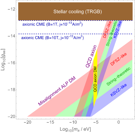
Figure 2: The axion parameter space that can be probed by the axionic chiral magnetic effect, if axion-induced electric current is measured up to $j=10^{-13}A/m^{2}$, assuming $v_{F}=0.01c$, and background magnetic field $B=1$T (upper dashed line) or $10$T (lower dashed line). Here $g_{ae}\equiv 2C_{e}m_{e}/f$. The brown shaded region is excluded by the brightness of the tip of the red-giant branch (TRGB) Capozzi:2020cbu ; Straniero:2020iyi . The red-green-blue shaded bands correspond to the parameter space for the QCD axion and axion-like particle dark matter from the misalignment mechanism. The yellow band is the parameter space where the QCD axion explains the total dark matter abundance with the initial misalignment angle $0.5<\theta_{i}<1.5$. For the ALP dark matter, we assume that the ALP mass is independent of temperature and the initial misaligned angle $\theta_{i}=1$. The red bands correspond to DFSZ-like models, the green bands for string-theoretic axions, and the blue bands for KSVZ-like models with the coefficient $C_{e}$ given in Eq. (6).

To conclude we show that the chiral magnetic effect is realized in a Fermi liquid of electrons by demonstrating that electric currents generate spontaneously along the external magnetic field if the medium is helicity imbalanced due to axion or axion-like dark matter. The CME is found to be suppressed by the Fermi velocity, in sharp contrast with the original result Fukushima:2008xe , which claims to be independent of the fermion mass, hence the Fermi velocity. We then propose to measure this spontaneous electric current in conductors to detect the axions or the axion-like particles. This effect exists even if the anomalous photon coupling is absent, as long as axions or axion-like particles couple to electrons, unlike the axion cavity experiments that assume the anomalous photon coupling of ADM. If this spontaneous electric current in medium is measured, it will strongly support the existence of axion or axion-like dark matter, telling us its possible microscopic origin.

- (1) See, for a recent review, K. Choi, S. H. Im and C. S. Shin, Ann. Rev. Nucl. Part. Sci. 71, 225-252 (2021).
- (2) F. Chadha-Day, J. Ellis and D. J. E. Marsh, Sci. Adv. 8, no.8, abj3618 (2022).
- (3) R. D. Peccei and H. R. Quinn, Phys. Rev. Lett. 38, 1440-1443 (1977).
- (4) S. Weinberg, Phys. Rev. Lett. 40, 223-226 (1978).
- (5) F. Wilczek, Phys. Rev. Lett. 40, 279-282 (1978).
- (6) J. Preskill, M. B. Wise and F. Wilczek, Phys. Lett. B 120, 127-132 (1983).
- (7) L. F. Abbott and P. Sikivie, Phys. Lett. B 120, 133-136 (1983).
- (8) M. Dine and W. Fischler, Phys. Lett. B 120, 137-141 (1983).
- (9) M. S. Turner, Phys. Rev. D 33, 889-896 (1986).
- (10) K. J. Bae, J. H. Huh and J. E. Kim, JCAP 09, 005 (2008).
- (11) P. Sikivie, Phys. Rev. Lett. 51, 1415-1417 (1983) [erratum: Phys. Rev. Lett. 52, 695 (1984)].
- (12) P. Sikivie, N. Sullivan and D. B. Tanner, Phys. Rev. Lett. 112, no.13, 131301 (2014).
- (13) R. Khatiwada et al. [ADMX], Rev. Sci. Instrum. 92, no.12, 124502 (2021).
- (14) Y. K. Semertzidis, J. E. Kim, S. Youn, J. Choi, W. Chung, S. Haciomeroglu, D. Kim, J. Kim, B. Ko and O. Kwon, et al. [arXiv:1910.11591 [physics.ins-det]].
- (15) S. Beurthey, N. Böhmer, P. Brun, A. Caldwell, L. Chevalier, C. Diaconu, G. Dvali, P. Freire, E. Garutti and C. Gooch, et al. [arXiv:2003.10894 [physics.ins-det]].
- (16) Y. Kahn, B. R. Safdi and J. Thaler, Phys. Rev. Lett. 117, no.14, 141801 (2016).
- (17) I. Obata, T. Fujita and Y. Michimura, Phys. Rev. Lett. 121, no.16, 161301 (2018).
- (18) D. J. E. Marsh, K. C. Fong, E. W. Lentz, L. Smejkal and M. N. Ali, Phys. Rev. Lett. 123, no.12, 121601 (2019).
- (19) A. Berlin, R. T. D’Agnolo, S. A. R. Ellis and K. Zhou, Phys. Rev. D 104, L111701 (2021).
- (20) J. Schütte-Engel, D. J. E. Marsh, A. J. Millar, A. Sekine, F. Chadha-Day, S. Hoof, M. N. Ali, K. C. Fong, E. Hardy and L. Šmejkal, JCAP 08, 066 (2021).
- (21) L. Krauss, J. Moody, F. Wilczek and D. E. Morris, Phys. Rev. Lett. 55, 1797 (1985).
- (22) Y. V. Stadnik and V. V. Flambaum, Phys. Rev. D 89, no.4, 043522 (2014).
- (23) C. Abel, N. J. Ayres, G. Ban, G. Bison, K. Bodek, V. Bondar, M. Daum, M. Fairbairn, V. V. Flambaum and P. Geltenbort, et al. Phys. Rev. X 7, no.4, 041034 (2017).
- (24) D. F. Jackson Kimball, S. Afach, D. Aybas, J. W. Blanchard, D. Budker, G. Centers, M. Engler, N. L. Figueroa, A. Garcon and P. W. Graham, et al. Springer Proc. Phys. 245, 105 (2020).
- (25) P. W. Graham, D. E. Kaplan, J. Mardon, S. Rajendran, W. A. Terrano, L. Trahms and T. Wilkason, Phys. Rev. D 97, no.5, 055006 (2018).
- (26) K. Fukushima, D. E. Kharzeev and H. J. Warringa, Phys. Rev. D 78, 074033 (2008).
- (27) D. K. Hong, Phys. Lett. B 699, 305-308 (2011).
- (28) K. Choi, S. H. Im, H. J. Kim and H. Seong, JHEP 08, 058 (2021).
- (29) B. Abelev et al. [ALICE], Phys. Rev. Lett. 110, no.1, 012301 (2013).
- (30) Q. Li, D. E. Kharzeev, C. Zhang, Y. Huang, I. Pletikosic, A. V. Fedorov, R. D. Zhong, J. A. Schneeloch, G. D. Gu and T. Valla, Nature Phys. 12, 550-554 (2016).
- (31) J. Ouellet and Z. Bogorad, Phys. Rev. D 99, no.5, 055010 (2019).
- (32) L. Brouwer, S. Chaudhuri, H. M. Cho, J. Corbin, C. S. Dawson, A. Droster, J. W. Foster, J. T. Fry, P. W. Graham and R. Henning, et al. [arXiv:2203.11246 [hep-ex]].
- (33) A. R. Zhitnitsky, Sov. J. Nucl. Phys. 31, 260 (1980).
- (34) M. Dine, W. Fischler and M. Srednicki, Phys. Lett. B 104, 199-202 (1981).
- (35) J. E. Kim, Phys. Rev. Lett. 43, 103 (1979).
- (36) M. A. Shifman, A. I. Vainshtein and V. I. Zakharov, Nucl. Phys. B 166, 493-506 (1980).
- (37) M. Srednicki, Nucl. Phys. B 260, 689-700 (1985).
- (38) S. Chang and K. Choi, Phys. Lett. B 316, 51-56 (1993).
- (39) M. Bauer, M. Neubert, S. Renner, M. Schnubel and A. Thamm, JHEP 04, 063 (2021).
- (40) Y. Aharonov and A. Casher, Phys. Rev. A 19, 2461-2462 (1979).
- (41) V. P. Gusynin, V. A. Miransky and I. A. Shovkovy, Phys. Rev. D 52, 4747-4751 (1995).
- (42) S. R. Coleman and B. Grossman, Nucl. Phys. B 203, 205-220 (1982).
- (43) C. Manuel, Phys. Rev. D 53, 5866-5873 (1996).
- (44) D. K. Hong, Phys. Lett. B 473, 118-125 (2000); Nucl. Phys. B 582, 451-476 (2000).
- (45) B. Feng, D. f. Hou, H. c. Ren and S. Yuan, Phys. Rev. D 103, no.5, 056004 (2021).
- (46) C. P. Salemi, J. W. Foster, J. L. Ouellet, A. Gavin, K. M. W. Pappas, S. Cheng, K. A. Richardson, R. Henning, Y. Kahn and R. Nguyen, et al. Phys. Rev. Lett. 127, no.8, 081801 (2021).
- (47) F. Capozzi and G. Raffelt, Phys. Rev. D 102, no.8, 083007 (2020).
- (48) O. Straniero, C. Pallanca, E. Dalessandro, I. Dominguez, F. R. Ferraro, M. Giannotti, A. Mirizzi and L. Piersanti, Astron. Astrophys. 644, A166 (2020).
- (49) C. P. Salemi, J. W. Foster, J. L. Ouellet, A. Gavin, K. M. W. Pappas, S. Cheng, K. A. Richardson, R. Henning, Y. Kahn and R. Nguyen, et al. Phys. Rev. Lett. 127, 081801 (2021).