Kernelization for Graph Packing and Hitting Problems
via Rainbow Matching

Abstract

We introduce a new kernelization tool, called rainbow matching technique, that is appropriate for the design of polynomial kernels for packing problems and their hitting counterparts. Our technique capitalizes on the powerful combinatorial results of [Graf, Harris, Haxell, SODA 2021]. We apply the rainbow matching technique on four (di)graph packing or hitting problems, namely the Triangle-Packing in Tournament problem (TPT), where we ask for a packing of $k$ directed triangles in a tournament, Directed Feedback Vertex Set in Tournament problem (FVST), where we ask for a (hitting) set of at most $k$ vertices which intersects all triangles of a tournament, the Induced 2-Path-Packing (I2PP) where we ask for a packing of $k$ induced paths of length two in a graph and Induced 2-Path Hitting Set problem (I2PHS), where we ask for a (hitting) set of at most $k$ vertices which intersects all induced paths of length two in a graph. The existence of a sub-quadratic kernels for these problems was proven for the first time in [Fomin, Le, Lokshtanov, Saurabh, Thomassé, Zehavi. ACM Trans. Algorithms, 2019], where they gave a kernel of $\mathcal{O}(k^{3/2})$ vertices for the two first problems and $\mathcal{O}(k^{5/3})$ vertices for the two last. In the same paper it was questioned whether these bounds can be (optimally) improved to linear ones. Motivated by this question, we apply the rainbow matching technique and prove that TPT and FVST admit (almost linear) kernels of $k^{1+\frac{\mathcal{O}(1)}{\sqrt{\log{k}}}}$ vertices and that I2PP and I2PHS admit kernels of $\mathcal{O}(k)$ vertices.

Keywords: Kernelization, Parameterized algorithms, Rainbow matching, Graph packing problems, Graph covering problems, Graph hitting problems.

1 Introduction

A parameterized problem $\Pi$ is a subset of $\Sigma^{*}\times\mathbb{N}$ for some finite alphabet $\Sigma.$ Given an instance $(x,k)$ of parameterized problem $\Pi$ we typically refer to $|x|$ as the size of the problem and to $k$ as the parameter of the problem and the general question of parameterized computation is whether $\Pi$ admits an algorithm able to decide, given an instance $(x,k)\in\Sigma^{*}\times\mathbb{N},$ whether $(x,k)\in$ in $f(k)\cdot|x|^{\mathcal{O}(1)}$ time. When this is indeed possible, then we say that is Fixed Parameter Tractable or, in short FPT. Parameterized computation was introduced by Downey and Fellows in their pioneering work in [17, 18, 15, 1, 16] and currently constitutes a fully developed discipline of Theoretical Computer Science (see [10, 21, 38, 19] for textbooks).

Kernelization algorithms. A particularly vibrant field of parameterized computation is kernelization. A kernelization algorithm for a parameterized problem $\Pi\subseteq\Sigma^{*}\times\mathbb{N}$ is a polynomial algorithm able to reduce every instance $(x,k)\in\Sigma^{*}\times\mathbb{N}$ to an equivalent one whose size depends exclusively on the parameter $k.$ If this size is bounded by a (polynomial) function $f(k),$ then we say that admits a (polynomial) kernel of size $f(k).$ The design of kernelization algorithms for parameterized problems has been a prominent topic of parameterized computation, mainly because it can be seen as a way to formalize preprocessing: when some parameterization of an NP-hard problem admits a kernel of size $f(k),$ then we may solve it by first applying, as a preprocessing step, the corresponding kernelization algorithm and then apply brute force techniques on a problem instance where the size $|x|$ of the problem has been radically reduced. Clearly, for small values of $k,$ this approach becomes particularly promising, especially when the problem in question admits a polynomial kernel. Unfortunately, not all parameterized problems are amenable to polynomial kernels and an extensive theory of kernelization has been developed so to either provide algorithmic techniques for the derivation of polynomial kernels (see e.g., [24, 28, 34, 35]) or to develop complexity-theoretic lower bound tools for kernelization [6, 20, 25, 31, 12, 14, 32] (see [23] for a dedicated textbook).

Greedy localization. A wide family of parameterized problems that have extensively studied from the kernelization point of view are (di)graph packing problems. Such problems are defined on graphs or digraphs and, typically, the question is whether an input (di)graph $G$ contains some collection of $k$ pairwise disjoint copies of some fixed (induced) sub(di)graph $H.$ A general approach for such problem is the greedy localization technique (see [11, 39]). This technique consists in finding, using some greedy approach, a maximal collection $\mathcal{C}$ of pairwise disjoint copies of $H$ in $G.$ If $\mathcal{C}$ has already at least $k$ elements, we may safely output a positive answer to the problem. If not, then we know that the $|H|(k-1)=\mathcal{O}(k)$ vertices of the (di)graphs in $\mathcal{C}$ should cover every possible solution of the problem. Based on this last covering property, the challenge is to design a polynomial time procedure that may discard all but a polynomial number of vertices from $G$ so that the remaining (di)graph is an equivalent instance. This procedure varies depending on the definition of the problem in question. Moreover, in case a polynomial kernel exists, a particular challenge towards deriving kernels of low polynomial size is to

maximize the set of discarded vertices so that the size of the resulting (di) graph, that is the output of the kernelization algorithm, is bounded by a low-polynomial function.

Rainbow matching technique. In this paper, we propose a framework for tackling the above challenge that we call the rainbow matching technique. Our technique capitalizes on the deep combinatorial results of Graf and Haxell in [27] (see also [26]). In fact, in Subsection 2.2, we derive the following “rainbow-matching” outcome of the main result of [27] asserting that there exists a polynomial time algorithm that, given an edge-multicolored graph $G$ (by $p$ colors), either outputs a matching of $G$ carrying all $p$ colors or outputs a non-empty set of colors $C\subseteq\{1,\ldots,p\}$ and a vertex set $X$ of size $\mathcal{O}(|C|)$ that intersects all edges colored by the colors of $C$ (Corollary 1).

For the purposes of our technique, we build an auxiliary graph based on the maximal solution $\mathcal{C}$ yielded by the greedy localization routine. We then consider a multi-coloring of the auxiliary graph based on the maximal solution $\mathcal{C}$. Depending of the outcome of the above algorithm, we either obtain an equivalent instance or we give a way to reorganize the parts of the (di)graph that are not in $\mathcal{C}$ in buckets in a way that will permit a recursive application of the above procedure until an equivalent instance is created. We provide a generic description of our technique in Section 3.

The rainbow matching technique seems to naturally apply to packing problems, where a maximum disjoint collection of a specific (di)graph $H$ is seeking in the input graph. We illustrate the technique on two packing problems. As a side effect, we notice that the technique also provides equivalent kernel for the corresponding dual problems of the considered ones. These hitting problems consist in finding a minimum set which intersects all the copies of $H$ in the input graph. In all, we apply the rainbow matching technique to four problems that we describe in the following.

Packing induced paths of length two. The first problem where our technique is applied is the following.

Induced 2-path-Packing (I2PP) Parameter: $k.$ Input: $(G,k)$ where $G$ is a graph and $k\in\mathbb{N}$ Question: Does $G$ contain $k$ pairwise disjoint induced paths of length two?

As in the case of TPT, the above problem admits a kernel on $\mathcal{O}(k^{2})$ vertices because of the results of Abu Khzam in [3, 2]. The first time a sub-quadratic kernel was given for I2PP was the one on $\mathcal{O}(k^{5/3})$ vertices by Fomin, Le, Lokshtanov, Saurabh, Thomassé, and Zehavi in [22]. Again, an open question that appeared in [22] is whether this bound can be improved to a linear one. As a second application of our technique, we prove that this is indeed the case.

Induced 2-paths Hitting Set. Given a grapĥ $G$, an induced 2-path hitting set of $G$ is a set $X$ which intersect all the induced 2-paths of $G$. In other words, $G\setminus X$ does not containany induced 2-path. Then, the dual version of the previous problem, on which we apply the rainbow matching technique, is the following.

Induced 2-paths Hitting Set (I2PHS) Parameter: $k.$ Input: $(G,k)$ where $G$ is a graph and $k\in\mathbb{N}$ Question: Is there an induced 2-paths hitting set of $G$ of size at least $k$?

Here again, this problem admits a kernel on $\mathcal{O}(k^{2})$ vertices because of the results of Abu Khzam in [4]. And the first sub-quadratic kernel for I2PHS was on $\mathcal{O}(k^{5/3})$ vertices given by Fomin, Le, Lokshtanov, Saurabh, Thomassé, and Zehavi in [22]. Here also, using our technique, we prove that I2PHS admits a linear kernel.

Packing directed triangles in tournament. The third problem we consider is the following .

Triangle-Packing in Tournament (TPT) Parameter: $k$ Input: $(T,k)$ where $T$ is a tournament and $k\in\mathbb{N}$ Question: Does $T$ contain $k$ pairwise disjoint directed triangles?

Recall that a directed graph $T=(V,E)$ is a tournament, if for every distinct $x,y\in V,$ either $(x,y)\in E$ or $(y,x)\in E$ holds (but not both).

The $\mathsf{NP}$-completeness of TPT follows from the results of [8]. Moreover, given that certain patterns are excluded from its inputs, it can be solved in polynomial time [7]. For (non) approximability results on the TPT problem see [29, 9, 36, 5]. Notice that TPT can directly be reduced to the 3-Hitting Set problem. For this problem, Abu Khzam gave, in [3, 2], a kernel on $\mathcal{O}(k^{2})$ vertices obtained by only removing vertices. This directly implies that TPT admits a kernel on $\mathcal{O}(k^{2})$ vertices. On the negative side, Bessy, Bougeret, and Thiebaut proved in [5] that TPT does not admit a kernel of (total bit) size $\mathcal{O}(k^{2-}),$ unless $\mathsf{NP}$ $\subseteq$co-NP/Poly. They also proved that TPT admits a kernel of $O(z)$ vertices, when its input instances are accompanied with a feedback arc set of $T$ of size $z$ and that TPT restricted to sparse tournaments admits a kernel of $O(k)$ vertices (i.e., of total bit-size $O(k\log{k})$). Towards breaking the quadratic bound in the general case, Fomin, Le, Lokshtanov, Saurabh, Thomassé, and Zehavi gave in [22] a kernel for TPT on $\mathcal{O}(k^{3/2})$ vertices. The open question of [22] is whether a kernel on $O(k)$ vertices exists for the general TPT. In this paper, we use the rainbow matching technique in order to give a kernel for TPT  on $k^{1+\frac{\mathcal{O}(1)}{\sqrt{\log{k}}}}$ vertices.

Feedback vertex set in tournament. The last problem on which we apply the rainbow matching technique is the dual version of the previous one and is described below. A triangle hitting set in a tournament $T$ is a set $X$ intersecting all the triangle of $T$. Equivalently, $T\setminus X$ does not contain any triangle and so, by a classical argument, is acyclic. Consequently, such a set $X$ is called a feedback vertex set of $T$.

Feedback Vertex Set in Tournament (FVST) Parameter: $k$ Input: $(T,k)$ where $T$ is a tournament and $k\in\mathbb{N}$ Question: Does $T$ contain a feedback vertex set of size at most $k$?

Here again, this problem admits a kernel on $\mathcal{O}(k^{2})$ vertices because of the results of Abu Khzam in [4]. And the first sub-quadratic kernel for FVST was on $\mathcal{O}(k^{3/2})$ vertices given by Fomin, Le, Lokshtanov, Saurabh, Thomassé, and Zehavi in [22]. Like for TPT, our technique leads us to obtain a kernel on $k^{1+\frac{\mathcal{O}(1)}{\sqrt{\log{k}}}}$ vertices for FVST.

Organization of the paper.

The definitions of the basic concepts that we use are given in Section 2. In the same section we present the combinatorial base of the rainbow coloring lemma (Corollary 1) as well as the proof of how this is derived by the results of [27]. In Section 3, we proceed with a generic description of our technique. An overview is presented in Subsection 3.1, while the main combinatorial assumptions and invariants are presented in Subsection 3.2 and Subsection 3.3. The description of the main algorithmic routine of the technique is given in Subsection 3.4. We then present specialization of the technique for I2PP in Section 4, for I2PHS in Section 5, for TPT in Section 6 and for FVST in Section 7. We chose to present the almost linear kernels for TPT and FVST after the linear ones for I2PP and I2PHS, as the application of the technique for the tournament problems is more technical. We conclude the paper in Section 8 with some remarks and open problems.

2 Definitions

We denote by $\mathbb{N}$ the set of non-negative integers and by $\mathbb{R}^{+}$ the set of all non-negative reals. Given two integers $p$ and $q,$ the set $[p,q]$ refers to the set of every integer $r$ such that $p\leq r\leq q.$ For an integer $p\geq 1,$ we set $[p]=[1,p],$ $[c]_{0}=[c]\cup\{0\},$ and $\mathbb{N}_{\geq p}=\mathbb{N}\setminus[0,p-1].$

For a set $S,$ we denote by $2^{S}$ the set of all subsets of $S$ and, given an integer $r\in[|S|],$ we denote by $\binom{S}{r}$ the set of all subsets of $S$ of size $r.$ Given two sets $A,B$ and a function $f:A\to B,$ for a subset $X\subseteq A$ we use $f(X)$ to denote the set $\{f(x)\mid x\in X\}.$

Finally, for every set of subsets $X_{i},$ $i\in[c],$ and any subset of indexes $I\subseteq[c],$ we denote $X_{I}=\bigcup_{i\in I}X_{i}$. And whenever we refer to a partition of a set $X$ into $c$ sets we refer to an (ordered) set $\mathcal{X}=\{X_{\ell}\mid\ell\in[c]\}$ where $V(\mathcal{X})=X$ and where we allow that some of the $X_{\ell}$’s is an empty set.

2.1 Basic concepts

Parameterized algorithms and kernels.

A parameterized problem $\Pi$ is a subset of $\Sigma^{*}\times\mathbb{N}$ for some finite alphabet $\Sigma.$ A parameterized problem $\Pi\subseteq\Sigma^{*}\times\mathbb{N}$ is fixed parameter tractable (in short fpt) if there is an algorithm that, given an instance $(x,k)\in\Sigma^{*}\times\mathbb{N},$ decides whether $(x,k)\in\Pi$ or not in time $f(k)\cdot p(|x|),$ where $f:\mathbb{N}\to\mathbb{N}$ is some function and $p\colon\mathbb{N}\to\mathbb{N}$ is a polynomial in the input size. The notion of kernelization is formally defined as follows.

Definition 1 (Kernelization).

Let $\Pi\subseteq\Sigma^{*}\times\mathbb{N}$ be a parameterized problem and $g$ be a computable function. We say that $\Pi$ admits a kernel of size $g$ if there exists an algorithm $\mathcal{K},$ called kernelization algorithm, or, in short, a kernel that given $(x,k)\in\Sigma^{*}\times\mathbb{Z}^{+},$ outputs, in time polynomial in $|x|+k,$ a pair $(x^{\prime},k^{\prime})\in\Sigma^{*}\times\mathbb{Z}^{+}$ such that

• $(x,k)\in\Pi$ if and only if $(x^{\prime},k^{\prime})\in\Pi,$ and

• $\max\{|x^{\prime}|,k^{\prime}\}\leq g(k).$

When $g(k)=k^{\mathcal{O}(1)}$ or $g(k)=\mathcal{O}(k)$ then we say that $\Pi$ admits a polynomial or linear kernel respectively. We refer to $g(k)$ as the size of the kernel produced by the kernelization algorithm.

When dealing with graphs algorithmic problems, the produced kernels are graphs, and we ofen refer to their size by specifying their number of vertices. For instance, we will say that a graph problem will admit a kernel with $\mathcal{O}(k)$ vertices (implicitely implying that the total size of the kernel is $\mathcal{O}(k^{2})$).

Graphs, digraphs and tournaments.

All graphs in this paper are finite. We use the term graph when we refer to an undirected graph without loops (ie. an edge with a unique endpoint) neither parallel edges (ie. distinct edges with the same endpoints). Also we use the term multigraph when we allow for loops and parallel edges. Directed graphs are called digraphs.

Given a (multi) (di)graph we denote by $V(G)$ and $E(G)$ the set of its vertices and edges respectively. Given a (multi) (di)graph $G$ and a set $X\subseteq V(G),$ we denote by $G[X]$ the sub(di)graph of $G$ induced by $X.$ Similarly, if $X\subseteq E(G),$ we use $G[X]$ in order to denote the graph $(V_{X},X),$ where $V_{X}$ is the set containing all the endpoints of the edges in $X.$ Given a graph (resp. digraph) $G$ and two disjoint subsets of vertices $A$ and $B,$ we say that $e\in E(G)$ is an edge (resp. arc) between $A$ and $B$ iff $|e\cap A|=|e\cap B|=1.$ In a digraph, whenever $(x,y)\in E(G),$ we say that $x$ dominates $y.$ We also say that a digraph $D$ is a tournament if, for every $\{x,y\}\in{V(D)\choose 2},$ either $(x,y)\in E(D)$ or $(y,x)\in E(D),$ but not both. If $\mathcal{S}=\{S_{1},\dots,S_{\ell}\}$ is a collection of vertex sets or subgraphs of some (multi) (di)graph, we denote by $V(\mathcal{S})$ the set $\bigcup_{i\in[\ell]}S_{i}$ or $\bigcup_{i\in[\ell]}V(S_{i})$ respectively. Given a (multi) (di)graph $G$ and $A\subseteq V(G),$ we denote by $G\setminus A$ the (multi) (di)graph $G[V(G)\setminus A]$ obtained after the deletion of all vertices of $A$.

2.2 Tools about rainbow matchings

Multigraph colourings.

Let ${G}$ be a multigraph. Recall that for $e\in E(G)$ we say that it is a loop of $G$ if $|e|=1,$ otherwise we say that it is an ordinary edge. A $p$-multiedge coloring of $G$ is a surjective function $\colon E(G)\rightarrow[p]$ that associates to each edge of $G$ a color in $[p]$ such that no two parallel edges of $G$ receive the same color. We call the pair $(G,)$ a $p$-edge colored multigraph and, given a set of colors $C\subseteq[p]$, we define $(G,)[C]=G[^{-1}(C)]$.

Given a $p$-edge colored multigraph $(G,)$, a rainbow matching of $(G,)$ is a set $X\subseteq E(G)$ such that

• $X$ is a matching of $G,$ i.e., every two distinct edges of $X$ are vertex-disjoint and

• $|X|=p$, and $(X)=[p]$.

For a subset $C\subseteq[p]$ of colors, recall that a set $X$ of vertices of $G$ is a vertex cover of $(G,)[C]$ iff for every $e\in E(G)$ where $(e)\in C,$ it holds that $e\cap X\neq\emptyset.$ We denote by $\textsf{vc}_{C}(G,)$ the minimum size of a vertex cover of $(G,)[C].$

The purpose of this section is to prove the following lemma.

Lemma 1.

Let $(G,)$ be a $p$-edge colored multigraph and $\in(0,1).$ If for every subset of colors $C\subseteq[p]$ we have $\textsf{vc}_{C}(G,)>(4+)(|C|-1),$ then $G$ contains a rainbow matching. Moreover there is an algorithm that, with input $(G,),$ either outputs a rainbow matching of $(G,)$ or a non-empty subset $C$ of $[p]$ and a vertex cover $X$ of $(G,)[C]$ such that $|X|\leq(4+)(|C|-1).$ This algorithm runs in time $\mathcal{O}(|V(G)|^{8}\cdot p^{f()}),$ for some function $f\colon\mathbb{N}\to\mathbb{N}.$

To prove Lemma 1, we only need a light version of Graf and Haxell’s Theorem, appeared as Theorem 4 in [27], which we present here (whose seminal version appeared in [30]).

Let $G$ be a graph enhanced with a partition $\mathcal{V}=(V_{1},\dots,V_{p})$ of its vertex set. An independent transversal of $G$ and $\mathcal{V}$ is an independent set $S$ of $G$ satisfying $|S\cap V_{i}|=1$ for every $i\in[p].$ For an integer $r,$ the graph $G$ is $r$-claw-free for $\mathcal{V}$ if no vertex of $G$ has $r$ independent neighbors in distinct sets $V_{i}.$ Finally, a set $X$ of $G$ is a dominating set of $G$ if for every vertex $v$ of $G$ there exists a vertex $x$ of $X$ such that $vx$ is an edge of $G.$

Theorem 1 (Graf and Haxell [27]).

For any fixed $r\in\mathbb{N}$ and $\in(0,1)$ there exists an algorithm that takes as input a graph $G$ and a partition $\mathcal{V}=(V_{1},\dots,V_{p})$ of its vertex set such that $G$ is $r$-claw-free for $\mathcal{V}$ and produces

• either an independent transversal of $G$ and $\mathcal{V},$ or

• a subset $I$ of $\{1,\dots,p\}$ and a set $X$ of vertices of $G$ such that $X$ is a dominating set of $G[\bigcup_{i\in I}V_{i}]$ and $|X|\leq(2+)(|I|-1).$

Moreover, the algorithm runs in $\mathcal{O}(|V(G)|^{4}\cdot p^{f(r,)})$ time, for some function $f\colon\mathbb{N}\times(0,1)\to\mathbb{N}.$

Proof of Lemma 1. Consider a $p$-edge colored multigraph $G$ and some $\in(0,1).$ We build an “extended line-graph” $G^{\prime}$ of $G$ in order to apply Theorem 1 on it. See Figure 1 for an example of construction. The graph $G^{\prime}$ is defined as follows:

$$V(G^{\prime})=\{(e,(e))\mid e\in E(G)\} E(G^{\prime})=\{\{(e,(e)),(e^{\prime},(e^{\prime}))\}\mid e\cap e^{\prime}\neq\emptyset\}.$$ and

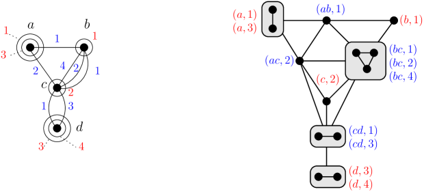
Figure 1: A $p$-edge-colored multigraph $G$ on the left where the sets of colors are shown in red for the loops and in blue for the ordinary edges of $G.$ On the right, the corresponding extended line-graph of $G,$ where the elements in red and in blue respectively correspond to loops and ordinary edges of $G.$

Notice that the size of $G^{\prime}$ is polynomial in the size of $G$ and $p,$ in particular $|V(G^{\prime})|=|E(G)|\leq\mathcal{O}(|V(G)|^{2}\cdot p).$ Notice also that $G^{\prime}$ is $3$-claw free, independently from the chosen partition of $\mathcal{V}.$ Indeed the neighborhood of every vertex $(e,(e))$ is either one clique (if $e$ is an loop) or the union of two cliques (if $e$ is an ordinary edge).

Now, consider the partition of the vertex set of $G^{\prime}$ given by the colors on the vertices of $G^{\prime},$ that is $V_{i}=\{(e,c_{0})\in V(G^{\prime})\mid c_{0}=i\},$ for $i\in[p].$ We then apply on $G^{\prime}$ the algorithm from Theorem 1 with $r=3$ and $/2$ as parameters. Clearly, this algorithm runs in time $\mathcal{O}(|V(G)|^{8}\cdot p^{f()}),$ for some function $f\colon\mathbb{N}\to\mathbb{N}.$

If we obtain an independent transversal of $G^{\prime},$ then it corresponds to a rainbow matching of $G.$

Suppose now that the algorithm outputs a subset $I$ of $[p]$ and a set $X$ of vertices of $G^{\prime}$ such that $X$ is a dominating set of $G^{\prime}[\bigcup_{i\in I}V_{i}]$ and $|X|\leq(2+/2)(|I|-1).$ Let $Y$ be the vertices of $G$ that are involved in an element of $X,$ that is $x\in Y$ if there exists $c_{0}$ such that $(\{x\},c_{0})\in X$ or there exist $c_{0}$ and $y\in V(G)$ such that $(\{x,y\},c_{0})\in X.$ We have $|Y|\leq 2|X|$ and we can claim that no edge $e$ of $G\setminus Y$ has a color from $I.$ Indeed, towards a contradiction, assume first that $e=\{x\}$ and $(e)=c_{0}\in I.$ As $X$ is a dominating set of $G^{\prime}[\bigcup_{i\in I}V_{i}],$ there exists an element $w$ of $X$ adjacent to $(\{x\},c_{0})$ in $G^{\prime}.$ If $w$ corresponds to a vertex of $G$ then, by construction of $G^{\prime},$ we have $w=(\{x\},c^{\prime})$ for a color $c^{\prime}\neq c_{0}.$ So, the vertex $x$ belongs to $Y,$ a contradiction. Now, if $w$ corresponds to an edge $e=\{u,v\}$ of $G,$ by construction of $G^{\prime},$ we have $u=x$ or $v=x$ and again the vertex $x$ belongs to $Y,$ a contradiction. Finally, assume that $e=\{x,y\}$ and $(e)\in I.$ Similarly, there exists an element $w$ of $X$ adjacent to $xy$ in $G^{\prime}.$ If $w$ corresponds to a vertex of $G,$ then it must be $x$ or $y,$ while if $w$ corresponds to an edge of $G,$ then this edge must have a common endpoint with $xy.$ In both cases, we have $x\in Y$ or $y\in Y,$ again a contradiction. So, $Y^{\prime}:=Y\cap V((G,)[I])$ is a vertex cover of $(G,)[I]$ and $|Y^{\prime}|\leq(4+)(|I|-1).$ $\square$

The rainbow coloring technique will be based on the following restatement of Lemma 1.

Corollary 1.

There exists some function $f\colon\mathbb{N}\to\mathbb{N}$ such that for every $>0$ there is an algorithm that, with input a $p$-edge-coloring graph $(G,),$ outputs either a rainbow matching of $(G,)$ or finds a non-empty subset $C$ of $[p]$ and a vertex cover $X$ of $(G,)[C]$ such that $|X|<(4+)|C|.$ Moreover, this algorithm runs in time $\mathcal{O}(|V(G)|^{8}\cdot p^{f()}).$

3 The rainbow matching technique

Both our kernelization algorithms for I2PP and TPT will be based on the the rainbow matching technique that we next describe in a generic form.

3.1 Overview of the kernelization algorithm

To that end, let us consider a generic $H$-packing problem (where $|H|=3$) where given an input $(G,k),$ the objective is to decide if there exist $k$ vertex disjoints sets $P_{i}\subseteq V(G)$ such that for any $i,$ $G[P_{i}]$ is isomorphic to $H.$ The rainbow matching technique that we introduce in this article can be summarized as follow. Given an input $(G,k)$:

1. Maintain a partition $(W,B,C)$ of $V(G)$ with size and structure invariants, called a partial decomposition, where $B\cup C$ is small (typically $\mathcal{O}(k)$), and $W$ is the large part where we want to select an approriate subset.

2. At each round, apply the following rule:

   • define an auxiliary edge-colored multigraph graph $(G,)\langle W,B,C\rangle$ with vertex set $W$.

   • applies Corollary 1 on $(G,)\langle W,B,C\rangle$:

     • if there exists a rainbow matching $M$ in $(G,)\langle W,B,C\rangle,$ stop the kernel and output $G[V(M)\cup B\cup C]$ (we selected $V(M)$ from $W$)

     • otherwise, use the subset of colors $X$ and its small vertex cover $T\subseteq W$ to compute a new partial decomposition $(W^{\prime},B^{\prime},C^{\prime})$

We point out that the partial decomposition may contain other information than $(W,B,C)$, as it is the case of example for TPT here, but for the sake of simplicity we stick to the triplet $(W,B,C)$ in this generic presentation. As invariants of a partial decomposition we used for I2PP and TPT have a lot of similarities, we now explain the common ideas behind these invariants.

3.2 Origin of the invariants in a partial decomposition.

We start with a greedy localization phase where we compute a maximal $H$-packing $\mathcal{P}=\{H_{1},\dots,$ $H_{i_{0}}\},$ and we assume that $i_{0}<k$ as otherwise we get a yes-instance. We define $C^{0}=V(\mathcal{P})$ and $W^{0}=V(G)\setminus C^{0}.$ Observe that there is no copy of $H$ inside $W^{0},$ and that $|C^{0}|=\mathcal{O}(k).$ The goal is to select a subset $S\subseteq W^{0}$ and to ouput $G[S\cup C^{0}].$ We want $S$ to be small, typically $|S|=\mathcal{O}(k),$ and safe, in the sense that any packing $\mathcal{P}$ in $G$ can be restructured into a packing $\mathcal{P^{\prime}}$ such that $|\mathcal{P^{\prime}}|\geq|\mathcal{P}|$ and $V(\mathcal{P^{\prime}})\subseteq S\cup C^{0}.$ This will imply that if $(G,k)$ is a yes-instance, then $(G[S\cup C^{0}],k)$ is also a yes-instance, and thus that these instances are equivalent as the other implication is straightforward.

Then, we define an auxiliary graph $(G,)\langle W^{0},\emptyset,C^{0}\rangle$ as follows (we used the $\langle W^{0},\emptyset,C^{0}\rangle$ notation to match notation of Section 3.1, as $B=\emptyset$ at the begining). Let $V((G,)\langle W^{0},\emptyset,C^{0}\rangle)=W^{0},$ and for any $c\in C^{0}$ and any $\{u,v\}\subseteq W^{0}$ such that $G[\{c,u,v\}]$ is isomorphic to $H,$ add to $(G,)\langle W^{0},\emptyset,C^{0}\rangle$ edge $e=\{u,v\}$ and set color $\chi(e)=c.$ Notice that $C^{0}$ both denotes a subset of vertices in $G$, and the set of colors of $(G,)\langle W^{0},\emptyset,C^{0}\rangle$ and this is a convention that we follow all over the paper. Now, apply Corollary 1 on $(G,)\langle W^{0},\emptyset,C^{0}\rangle,$ and let us discuss the two possible outcomes of this corollary.

Case where a rainbow matching exists.

We now consider te case where we have a rainbow matching $M$ in $(G,)\langle W^{0},\emptyset,C^{0}\rangle.$ In this case, we stop and return $G[V(M)\cup C^{0}].$ Observe first that $V(M)$ is small, as $|V(M)|=2|C^{0}|=\mathcal{O}(k).$ Let us now examine why it is safe. Consider an $H$-packing $\mathcal{P}$ in $G.$ We restructure $\mathcal{P}$ as follows (see Figure 2). For any $H_{i}\in\mathcal{P}$ we define a corresponding $H^{\prime}_{i}$ as follows (and we define $\mathcal{P}^{\prime}=\{H^{\prime}_{i}\mid H_{i}\in\mathcal{P}\}$):

• If $H_{i}\subseteq C^{0},$ define $H^{\prime}_{i}=H_{i}.$

• Otherwise, we know that $H_{i}\cap C^{0}\neq\emptyset$ by the maximality of the greedy localization. Let $c\in H_{i}\cap C^{0},$ and $e_{c}=\{u_{c},v_{c}\}$ the edge of $M$ such that $\chi(e_{c})=c.$ Restructure $H_{i}$ into $H^{\prime}_{i}=\{c,u_{c},v_{c}\}.$

We can observe that the $\{H^{\prime}_{i}\}$ are vertex disjoint as $M$ is a matching, and thus that $V(M)$ is safe.

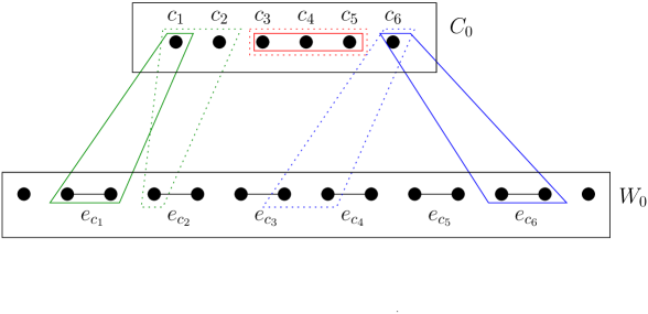
Figure 2: An example showing how to restructure $H^{\prime}_{1},H^{\prime}_{2},H^{\prime}_{3}$ (in dashed lines) to $H_{1},H_{2},H_{3}$ (in plain lines) using the rainbow matching $\{e_{c_{i}},1\leq i\leq 6\}.$

Case where a small vertex cover exists.

Suppose there exists a subset of colors $X\subseteq C^{0}$ and a vertex cover $T$ of $(G,)\langle W^{0},\emptyset,C^{0}\rangle[X]$ such that $|T|\leq(4+)|X|.$ Let $B=T\cup X,$ $W=W^{0}\setminus T,$ and $C=C^{0}\setminus X.$ Observe that as $T$ is a vertex cover of $(G,)\langle W^{0},\emptyset,C^{0}\rangle[X],$ for any set $H^{\prime}\subseteq B\cup W$ such that $G[H^{\prime}]$ is isomorphic to $H,$ we have $|H^{\prime}\cap W|\leq 1.$ This crucial property will help us to control how copies of $H$ can be packed in $G[W\cup B],$ and thus motivates the invariants required in the following (informal) definition of partial decomposition.

3.3 Invariants in a partial decomposition

We say that $(W,B,C)$ is a partial decomposition (with respect to $(C^{0},W^{0})$) of $G$ if

1. $W,B,C$ is a partition of $V(G)$

2. $(W,B)$ is a nice pair: $W\subseteq W^{0}$ and for any $H^{\prime}\subseteq B\cup W$ such that $G[H^{\prime}]$ is isomorphic to $H,$ $|H^{\prime}\cap W|\leq 1$

3. (size invariant) $B$ is small (typically $|B|=\mathcal{O}(|C^{<}|),$ where $C^{<}=C^{0}\setminus C$

As $C^{0}$ and $W^{0}$ will be fixed (there are only computed once at the begining), we voluntarily do not mention “with respect to $(C^{0},W^{0})$” in the reminder of the article. Observe that the tuple $(W,B,C)$ that we obtained at this end of Section 3.2 is a partial decomposition. Properties 1 and 2 listed above are common to both problems, whereas the notion of size to ensure that $B$ is small is ad-hoc (but with the same objective to guarantee that $|B|+|C|=\mathcal{O}(|C^{0}|),$ as $B$ and $C$ will be part of the output of the kernel). The property of being a nice pair will allow us to provide a structural description of $B$: in both problems we will partition $B$ into buckets $B_{i},$ and obtain a description on how copies of $H$ in $W\cup B$ intersect the buckets.

3.4 Description of one round of the kernel

We now consider an arbitrary round of the kernel, where we have our current partial decomposition $(W,B,C).$ The objective is now to apply again Corollary 1, but in a more general setting than in Section 3.2 where we had $B=\emptyset.$

Let us now discuss how to define the auxiliary graph $(G,)\langle W,B,C\rangle.$ We start as before by defining $V((G,)\langle W,B,C\rangle)=W,$ and for any $c\in C,$ and any $\{u,v\}\subseteq W$ such that $G[\{c,u,v\}]$ is isomorphic to $H,$ adding to $(G,)\langle W,B,C\rangle$ edge $e=\{u,v\}$ and set $\chi(e)=c.$ Again, notice that according to the context, $C$ may denote a subset of $G$, of a subset of our colors in $(G,)\langle W,B,C\rangle$. The crux of this approach is to add to $(G,)\langle W,B,C\rangle$ some loops in $W$ and a coloring of these loops (using a fresh set of colors $D,$ which is disjoint from $C$), such that:

1. $|D|=\mathcal{O}(|B|)$

2. if there exists a rainbow matching $M^{D}$ only for loops of colors in $D$ (meaning that $M^{D}=\{v_{d},d\in D\}$ and $|M^{D}|=|D|$), then for any packing $\mathcal{P}$ of $G[W\cup B],$ there exists a packing $\mathcal{P^{\prime}}$ such that $|\mathcal{P^{\prime}}|=|\mathcal{P}|$ and $V(\mathcal{P^{\prime}})\subseteq B\cup V(M^{D})$

3. if there exists a subset of colors $X^{D}\subseteq D$ and a vertex cover $T$ of $(G,)\langle W,B,C\rangle[X^{D}]$ such that $|T|\leq 2(4+)|X^{D}|,$ then we can find in polynomial time a non-empty subset $T^{\prime}\subseteq T$ such that we can add $T^{\prime}$ to $B$ without violating the size invariant of a partial decomposition. In other words, in this case we define $W^{\prime}=W\setminus T^{\prime},$ $B^{\prime}=B\cup T^{\prime},$ $C^{\prime}=C,$ and we want that $(W^{\prime},B^{\prime},C^{\prime})$ remains a partial decomposition.

The way we can define such colored loops to obtain the three previous properties depends on the problem that we consider and thus will be specified in each application of the technique. As we guess that, at a first sight, Property iii. may look like it comes out of nowhere, let us now explain why properties i. to iii. are sufficient to obtain the kernel. Suppose that we defined an auxiliary graph $(G,)\langle W,B,C\rangle$ satisfying the previous properties, and that we apply Corollary 1 on $(G,)\langle W,B,C\rangle.$ Let us discuss again the two possible outcomes of this Corollary.

Case where a rainbow matching exists.

Consider now the case where there is a rainbow matching $M$ in $(G,)\langle W,B,C\rangle.$ In this case, we stop and return $G[V(M)\cup B\cup C].$ Let us partition $M=M^{C}\cup M^{D},$ where $M^{C}$ (resp. $M^{D}$) are edges whose color is in $C$ (resp. $D$). Observe first that the kernel output is small, as $|V(M)|=|D|+2|C|=\mathcal{O}(|B|+|C|)$ (by Property i.), and thus the output has vertex size $\mathcal{O}(|B|+|C|)=\mathcal{O}(|C^{<}|+|C|)=\mathcal{O}(|C^{0}|)=\mathcal{O}(k)$ (by Property 3). Let us now examine why it is safe. Consider an $H$-packing $\mathcal{P}$ in $G.$ We restructure $\mathcal{P}$ as follows (see Figure 3). For any $H_{i}\in\mathcal{P}$ we define a corresponding $H^{\prime}_{i}$ as follows (and we define $\mathcal{P}^{\prime}=\{H^{\prime}_{i}\mid H_{i}\in\mathcal{P}\}$):

• If $H_{i}\subseteq C,$ define $H^{\prime}_{i}=H_{i}.$

• If $H_{i}\nsubseteq C,$ and $H_{i}\cap C\neq\emptyset,$ choose $c\in H_{i}\cap C,$ and define $e_{c}=\{u_{c},v_{c}\}$ the edge of $M$ such that $\chi(e_{c})=c.$ Restructure $H_{i}$ into $H^{\prime}_{i}=\{c,u_{c},v_{c}\}.$

• Now, it only remains to restructure $\mathcal{P}_{(W\cup B)}=\{H_{i}\in\mathcal{P}\mid H_{i}\subseteq W\cup B\}.$ By Property ii., there exists a packing $\mathcal{P^{\prime}}_{(W\cup B)}$ such that $|\mathcal{P^{\prime}}_{(W\cup B)}|=|\mathcal{P}_{(W\cup B)}|$ and $V(\mathcal{P^{\prime}}_{(W\cup B)})\subseteq B\cup V(M^{D}).$

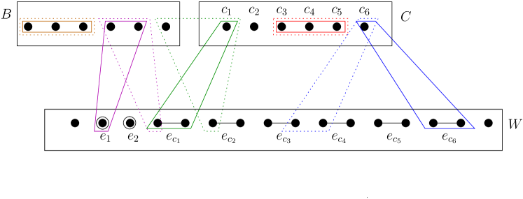
Figure 3: The color set of $(G,)\langle W,B,C\rangle$ is $C\cup D$, where here $C=\{c_{1},\dots,c_{6}\}$, and $D=\{d_{1},d_{2}\}$ (where $D\cap C=\emptyset$). In this example we assume that there exists a rainbow matching $M$ in $(G,)\langle W,B,C\rangle$. We have $M=M^{C}\cup M^{D},$ where $M^{C}=\{e_{c_{i}},1\leq i\leq 6\}$ and $M^{D}=\{e_{1},e_{2}\}.$ Here, we restructure $H^{\prime}_{1},H^{\prime}_{2},H^{\prime}_{3},H^{\prime}_{4},H^{\prime}_{5}$ (in dashed lines) to $H_{1},H_{2},H_{3},H_{4},H_{5}$ (in plain lines) according to $M$.

We can observe that the $\{H^{\prime}_{i}\}$ are vertex disjoint as $M$ is a matching, and thus that $V(M)$ is safe. Observe that the matching was computed without considering the complex (and unknown) structure of “bad” copies of $H$ that use vertices of both $B$ and $C.$ In other words, the way we organize the previous restructuration allows us to forget these bad copies in $G.$

Case where a small vertex cover exists.

Suppose there exists a non-empty subset of colors $X\subseteq C\cup D$ and a vertex cover of $T$ of $(G,)\langle W,B,C\rangle[X]$ such that $|T|\leq(4+)|X|.$ Let $X^{C}=X\cap C$ and $X^{D}=X\cap D.$. Notice first that we cannot simply proceed as in Section 3.2 (where $X^{D}$ was empty) and define $W^{\prime}=W\setminus T,$ $C^{\prime}=C\setminus X^{C}$ and $B^{\prime}=B\cup(T\cup X^{C}).$ Indeed, if we want the size property 3 to be respected, we need that what we add to $B$ is linear in what we remove from $C,$ or more formally that $|T\cup X^{C}|=\mathcal{O}(|X^{C}|).$ However, we only know that $|T|\leq(4+)|X|=(4+)(|X^{D}|+|X^{C}|),$ and thus if $|X^{C}|$ is small compared to $|X^{D}|$ (typically $|X^{C}|=0$), we don’t have the property we need. This is where we use (for both problems) the following win/win trick.

Case 1: if $|X^{D}|\leq|X^{C}|.$ In this case, the previous inequality gives us $|T|\leq(4+)|X|=2(4+)|X^{C}|,$ and we can define $W^{\prime}=W\setminus T,$ $C^{\prime}=C\setminus X^{C}$ and $B^{\prime}=B\cup(T\cup X^{C})$ while preserving size Property 3. Notice that the crucial property ensuring that $(W^{\prime},B^{\prime})$ is still a nice pair (which is required to obtain that $(W^{\prime},B^{\prime},C^{\prime})$ remains a partial decomposition) is that there is no $H^{\prime}$ such that $G[H^{\prime}]$ is isomorphic to $H$ where $|H^{\prime}\cap W^{\prime}|=2$ and $|H^{\prime}\cap X^{c}|=1,$ which holds because $T$ is a vertex cover of $(G,)\langle W,B,C\rangle[X]$.

Case 2: if $|X^{D}|>|X^{C}|.$ In this case, the previous inequality gives us $|T|\leq 2(4+)|X^{D}|,$ and we use Property iii. to find in polynomial time a non-empty subset $T^{\prime}\subseteq T$ such that $(W^{\prime},B^{\prime},C^{\prime})$ remains a partial decomposition, where $W^{\prime}=W\setminus T^{\prime},$ $B^{\prime}=B\cup T^{\prime},$ $C^{\prime}=C.$ Thus, Case 2 corresponds to a case where we discover that a certain part $T^{\prime}\subseteq W$ is small, and can be added to the buckets.

Notice that in both Cases 1 and 2, we obtain a new “smaller” partial decomposition where either $|C^{\prime}|<|C|$ (because $X^{C}$ is non-empty, in Case 1) or $|W^{\prime}|<|W|$ (in Case 2). Thus the algorithm terminates.

3.5 Applicability of the rainbow coloring technique

The rainbow matching technique consists in applying the algorithm of Section 3.1. Adapting this technique to a particular problem requires to find a way to define colors for buckets that respects Properties i., ii., and iii., together with a notion of size used in Property 3. In Section 4 and Section 6, we present how this technique can be applied for I2PP and TPT respectively.

4 Linear kernel for I2PP

4.1 Notation

Given a graph $G$ we refer to a path in $G$ of length 2 as a 2-path of $G.$ We say that a 2-path of $G$ is induced if there is no edge in the graph between its endpoints. We call a $P_{3}$ an induced 2-path. When we refer to a $P_{3}$ in a graph, we will see it as a subset of vertices rather than an induced subgraph. An induced $P_{3}$-packing of $G$ is a set $\mathcal{P}=\{V_{i},i\in[x]\}$ of vertex-disjoint induced $P_{3}$’s.

Induced 2-path-Packing (I2PP) Parameter: $k.$ Input: $(G,k)$ where $G$ is a graph and $k\in\mathbb{N}$ Question: Is there an induced $P_{3}$-packing of size at least $k$?

In this section we prove the following theorem.

Theorem 2.

There exists some function $f:\mathbb{N}\to\mathbb{N}$ such that for every $>0,$ there exists an algorithm that, given an instance $(G,k)$ of I2PP outputs a set $A\subseteq V(G)$ such that $(G[A],k)$ is an equivalent instance where $|A|\leq(243+)k.$ Moreover this algorithm runs in time $\mathcal{O}(|V(G)|^{f()}).$ In other words, I2PP admits a kernel of a linear number of vertices.

4.2 Preliminary phase: greedy localization

Given an input $(G,k)$ of I2PP, we start by a greedy localization phase, that is, by finding, in polynomial time, an inclusion-wise maximal induced 2-path-packing of $G.$ Let $C^{0}$ be the set of the vertices in the paths of such a packing. If $|\mathcal{P}^{0}|\geq k$ we can directly answer that $(G,k)$ is a yes-instance, therefore we may suppose that $|P^{0}|<k,$ implying that $|C^{0}|\leq 3(k-1).$ The vertices of $C^{0}$ will be referred as (distinct) colors. Observe that as the considered induced 2-path-packing is inclusion-wise maximal, the graph $W^{0}:=G\setminus C^{0}$ does not contain $P_{3}$ as an induced subgraph, consequently it is the disjoint union of a set, say $\mathcal{W}^{0}=\{W^{0}_{1},\ldots,W^{0}_{i_{0}}\},$ such that, for $i\in[i_{0}],$ the graph $G[W_{i}^{0}]$ is a clique. Clearly, $V(G)=C^{0}\cup V(\mathcal{W}^{0})$ and, for any $\{i,i^{\prime}\}\in{[i_{0}]\choose 2},$ there is no edge between $W^{0}_{i}$ and $W^{0}_{i^{\prime}}.$ Such a couple $(C^{0},\mathcal{W}^{0})$ will be referred as a greedy localized pair for the input $(G,k)$.

This completes the initialization phase, and the tuple $(C^{0},\mathcal{W}^{0})$ will be given as initial input of our kernelization algorithm.

4.3 Nice pair, buckets, partial decomposition, and auxiliary graph

In all this section we consider that we are given an input $(G,k)$ of I2PP, and a greedy localized pair $(C^{0},\mathcal{W}^{0})$ for input $(G,k).$ Recall that $\mathcal{W}^{0}=\{W^{0}_{1},\ldots,W^{0}_{i_{0}}\}$ and $W^{0}=V(\mathcal{W}^{0}).$

Figure 4: Example of a bucket decomposition and a partial decomposition. The vertex depicted in $B_{2}$ is adjacent to all vertices of $W_{2}$, and not adjacent to any other vertex in $W$. We depict the case where the kernelization algorithm does not find a rainbow matching in $(G,)\langle W,B,C\rangle$ and therefore it finds a subset of colors $X$ (depicted in blue) along with a small set of vertices $T$ (depicted in green) such that $T$ is a vertex cover of $(G,)\langle W,B,C\rangle[X].$

Given two disjoint subsets $W$ and $B$ of $V(G),$ we say that the pair $(W,B)$ is a nice pair of $G$ if $W\subseteq W^{0}$ and if every induced 2-path of $B\cup W$ contains at most one vertex in $W.$

Bucket decompositions. Given two disjoints subsets $W$ and $B$ of $V(G),$ a bucket decomposition (see Figure 4) of the pair $(W,B)$ is defined by the following three partitions:

• a partition $\{B_{\neq\emptyset},B_{\emptyset}\}$ of $B$

• a partition $\{B_{1},\ldots,B_{i_{0}}\}$ of $B_{\neq\emptyset},$ (we call the sets of this partition buckets) and

• a partition $\{W_{1},\ldots,W_{i_{0}}\}$ of $W.$

(recall that we allow empty sets in partitions)

such that

1. for $i\in[i_{0}]$ $W_{i}=W\cap W^{0}_{i}$

2. $B_{\emptyset}=\{v\in B\mid N_{G}(v)\cap W=\emptyset\}$ and $B_{\neq\emptyset}=\{v\in B\mid N_{G}(v)\cap W\neq\emptyset\}$

3. for any $i\in[i_{0}]$ and $v\in B_{i},$ $N_{G}(v)\cap W=W_{i}$ (the neighborhood in $W$ of any vertex of a bucket $B_{i}$ is exactly the vertex set of its “corresponding” clique $G[W_{i}]$).

We denote $F=\{i\in[i_{0}]\mid W_{i}=\emptyset\},$ $\bar{F}=[i_{0}]\setminus F.$ Observe that if $W_{i}=\emptyset,$ then $B_{i}=\emptyset,$ as vertices in $B_{i}$ belong to $B_{\neq\emptyset}$ and should have $N(v)\cap W\neq\emptyset.$ The contrapositive is not true as we may have $W_{i}\neq\emptyset$ and $B_{i}=\emptyset.$

Lemma 2.

Given $W$ and $B$ disjoint subsets of $G,$

1. $(W,B)$ is a nice pair iff it admits a bucket decomposition.

2. if $(W,B)$ is nice pair, then for any induced 2-path $P$ in $G$ such that $P\subseteq W\cup B,$ $P\cap W\neq\emptyset,$ there exists a unique $i\in[i_{0}]$ and vertices $u,v,w$ such that $P=\{u,v,w\},$ $u\in B,$ $v\in B_{i}$ and $w\in W_{i}.$ Informally, $P$ must have exactly one vertex in one of the remaining cliques, one in its corresponding bucket, and the last one anywhere in $B.$

Proof.

We start with the proof of the first item.
($\Rightarrow$) Suppose $(W,B)$ is a nice pair. Consider a vertex $v\in B_{\neq\emptyset}.$ There exists $i\in[i_{0}]$ such that $N(v)\cap W_{i}\neq\emptyset.$ Let $u\in N(v)\cap W_{i}.$ If there existed $w\in W_{i}$ such that $w\notin N(v),$ then, as $W_{i}$ is a clique, we would have that $P=\{v,u,w\}$ is an induced 2-path such that $|P\cap W|\geq 2,$ a contradiction. This implies that $N(v)\cap W\supseteq W_{i}.$ Let us now prove that $N(v)\cap W=W_{i}$. Suppose, towards a contradiction, that there exists $j\neq i$ and $u^{\prime}\in N(v)\cap W_{j}.$ Then, as there is no edges between $W_{j}$ and $W_{i},$ we obtain that $P=\{v,u,u^{\prime}\}$ is an induced 2-path such that $|P\cap W|\geq 2,$ a contradiction. Thus, we obtain the partition $\{B_{1},\ldots,B_{i_{0}}\}$ of $B_{\emptyset},$ where $B_{i}=\{i\in B_{\neq\emptyset}\mid N(v)=W_{i}\}$ (some of the $B_{i}$’s may be empty).

($\Leftarrow$) Let $(W,B)$ be a pair admiting a bucket decomposition. Let us prove the following structural property: for any $P$ induced 2-path of $G[W\cup B]$ such that $P\cap W\neq\emptyset,$ there exists a unique $i\in i_{0}$ and vertices $u,v,w$ such that $P=\{u,v,w\},$ $u\in B,$ $v\in B_{i},$ and $w\in W_{i}.$ We cannot have $P\subseteq W$ as $W$ is a union of cliques (as $W_{i}\subseteq W_{i}^{0}$), implying that $P\cap B\neq\emptyset.$ This implies that there exists an edge $\{v,w\}\subseteq P$ such that $v\in B$ and $w\in W.$ By Property 2, we know that $v\notin B_{\emptyset},$ implying that there exists $i\in[i_{0}]$ such that $v\in B_{i}.$ Property 3 implies that $w\in W_{i}.$ Let us now consider the third vertex $u$ of $P.$ Firstly, $u$ cannot be in $W_{i}$ as, by Property 3, this would imply that $\{v,u\}$ is an edge, and thus $P$ would be a triangle. Secondly, $u$ cannot be in a $W_{j},$ where $j\neq i,$ as by Property 3, $N(v)\cap W=W_{i}.$ This implies that $u\in B$ and concludes the proof of the structural property. The fact that $(W,B)$ is a nice pair is now immediate.

The second item immediately follows. Indeed, by the first part of the result, any nice pair $(W,B)$ admits a bucket decomposition, which implies the structural property as seen previously. ∎

Given a nice pair $(W,B),$ we will refer to $B_{\emptyset},$ $B_{\neq\emptyset},$ $F$ and $\bar{F}$ as defined in the bucket decomposition. Informally, $F$ will denote the set of indexes of cliques that will survive during the course of the kernelization algorithm. Recall that, using our notations, $B_{\bar{F}}=\bigcup_{i\in\bar{F}}B_{i}$ and observe that $B_{\bar{F}}=B_{\neq\emptyset}.$

We fix some $>0$ and set $c_{1}=4+$ ($c_{1}$ is suited so to permit the application of Corollary 1). Given a nice pair $(W,B),$ we define the size of $(W,B)$ as

$$s(W,B)=\frac{|B_{\emptyset}|}{1+2c_{1}}+|B_{\neq\emptyset}|.$$

Definition 2.

We say that a tuple $(W,B,C)$ is a partial decomposition iff:

Partition requirements:
Let $C^{<}=C^{0}\setminus C$ (which we will see as the colors already treated by previous applications of the rule of the kernelization algorithm)

1. there is a partition $V(G)=W\cup B\cup C,$

2. $C\subseteq C^{0},$ and

3. $(W,B)$ is a nice pair.

Size requirement:

1. $s(W,B)\leq(1+2c_{1})|C^{<}|.$

Moreover, we will say that the partial decomposition is clean if it satisfies the following extra condition:

1. for every vertex $c\in C$ the graph $G[W\cup\{c\}]$ contains an induced 2-path.

The initial partial decomposition we will consider (which will be $(W_{0},\emptyset,C_{0})$) as well as partial decompositions which will be produced by our kernelization procedure will not necessarily be clean partial decompositions. However the simple following lemma allows to clean a partial decomposition.

Lemma 3 (Cleaning Lemma).

Let $(W,B,C)$ be a partial decomposition and $X$ be set the of vertices $x$ of $C$ such that $G[W\cup\{x\}]$ does not contain any induced 2-path. Then $(W,B\cup X,C\setminus X)$ is a clean partial decomposition.

Proof.

First let us check that $(W,B\cup X,C\setminus X)$ satisfies the requirements of a partial decomposition. Properties 1 and 2 are clearly satisfy, and by choice of $X$, no vertex of $X$ is contained in an induced 2-path with two vertices of $W$, so $(W,B\cup X)$ is also a nice pair and property 3 is satisfies. To conlude that $(W,B\cup X,C\setminus X)$ is a partial decomposition, let us check it fulfills the size requirement. Indeed each time one vertex of $X$ is added to $B$, $s(W,B)$ increases by at most 1, whereas $(1+2c_{1})|C^{<}|$ increases by $1+2c_{1}$. So, the size requirement 1 is still valid. By repeating this counting argument for every vertex of $X$, we can conclude that $(W,B\cup X,C\setminus X)$ is a partial decomposition. Moreover, it is clear that every vertex of $C\setminus X$ forms an induced 2-path with two vertices of $W$ and that $(W,B\cup X,C\setminus X)$ is clean. ∎

Definition 3 (Auxiliary graph).

Let $(W,B,C)$ be a partial decomposition. Let $p=|C|+\sum_{i\in[i_{0}]}|B_{i}|.$ We define the $p$-edge-colored multigraph $(\tilde{G},)\langle W,B,C\rangle$ where the vertex set of $\tilde{G}$ is $W$ and the edges of $\tilde{G},$ as well as their colors, are defined as follows. For any $i\in\bar{F}$ and any $u\in B_{i}$ and for any $v\in W_{i},$ we add an edge $e=\{v\}$ and we set $(e)=u.$ Moreover, for any $u\in C$ and for any $v$ and $w$ in $W$ such that $\{u,v,w\}$ is an induced 2-path, we add an edge $e=\{v,w\}$ and we set $(e)=u.$

Observe that an edge $\{v,w\}$ of $(\tilde{G},)\langle W,B,C\rangle$ can be either inside a $W_{i}$ (in this case $\{v,w\}$ is also an edge in $G$ as $G[W_{i}]$ is a clique) or between $W_{i}$ and $W_{i^{\prime}}$ for $i\neq i^{\prime}$ (in this case $\{v,w\}$ is a non-edge in $G$). Notice that if $W=\emptyset,$ then $(\tilde{G},)\langle W,B,C\rangle$ is the empty graph and we consider that it admits a rainbow matching $M=\emptyset.$ Notice also that $C$ or $B_{\neq\emptyset}$ may be empty. If $C=B_{\neq\emptyset}=\emptyset$ then $(\tilde{G},)\langle W,B,C\rangle$ has no edges and we consider that it admits a rainbow matching $M=\emptyset$ (but this case will not occur), however cases where one of the two sets $C,$ $B_{\neq\emptyset}$ is empty will occur in the kernel.

4.4 Analysis of the two cases: rainbow matching or small vertex cover

First, let us look at the case where the reduction rule produces a rainbow matching.

Lemma 4 (Case of rainbow matching).

Let $(W,B,C)$ be a clean partial decomposition. Suppose that the colored multigraph $(\tilde{G},)\langle W,B,C\rangle$ admits a rainbow matching $M$. Let $A=V(M)\cup B\cup C,$ and $G^{\prime}=G[A].$ Then,

1. $(G,k)$ and $(G^{\prime},k)$ are equivalent instances of I2PP,

2. $|A|\leq 3(1+2c_{1})^{2}k.$

Proof.

Equivalence property. First, if $W=\emptyset,$ then $(\tilde{G},)\langle W,B,C\rangle$ is the empty graph then $M=\emptyset$ and $G^{\prime}=G,$ implying the equivalence. Let us now assume that $W\neq\emptyset.$ Let us assume that $(G,k)$ is yes-instance and prove that $(G^{\prime},k)$ is as well (the other direction is straightforward as $G^{\prime}$ is an induced subgraph of $G$). Let $\mathcal{P}^{*}=\{P^{*}_{i},i\in[k]\}$ be an induced $P_{3}$-packing in $G$ of size $k.$

Notice that the only vertices of $G$ not belonging to $G^{\prime}$ are in $W.$ Let us partition $\mathcal{P}^{*}=\mathcal{P}^{*}_{1}\cup\mathcal{P}^{*}_{W},$ where $\mathcal{P}^{*}_{W}=\{P\in\mathcal{P}^{*}\mid P\cap W\neq\emptyset\}.$ Our objective is to restructure $\mathcal{P}^{*}$ into another induced 2-path-packing $\mathcal{P}=\mathcal{P}^{*}_{1}\cup\mathcal{P}_{W}$ such that $|\mathcal{P}_{W}|=|\mathcal{P}^{*}_{W}|.$ To that end, we will associate to each $P^{*}_{i}\in\mathcal{P}^{*}_{W}$ a set $P_{i}\in\mathcal{P}_{W}$ such that

1. for any $P_{i}\in\mathcal{P}_{W},$ $P_{i}$ is an induced 2-path in $G^{\prime}$

2. for any $P_{i},P_{j}$ in $\mathcal{P}_{W},$ $P_{i}\cap P_{j}=\emptyset$ (paths in ${\cal P}_{W}$ are vertex-disjoint)

3. for any $i,$ $P_{i}\cap(V(G)\setminus W)\subseteq P^{*}_{i}\cap(V(G)\setminus W)$ (roughly speaking outside $W,$ path $P^{*}_{i}$ uses more vertices than $P_{i}$)

Observe that Properties 2 and 3 imply that paths in $\mathcal{P}$ are vertex-disjoint. In particular, if, towards a contradiction, a path $P\in\mathcal{P}^{*}_{1}$ intersected a path $P_{i}\in\mathcal{P}_{W},$ then, by Property 3, we would also have $P\cap P^{*}_{i}\neq\emptyset,$ which is a contradiction. Let us now define the $P_{i}$’s.

Let us partition $\mathcal{P}^{*}_{W}=\mathcal{P}^{*}_{CW}\cup\mathcal{P}^{*}_{\bar{C}W},$ where $\mathcal{P}^{*}_{CW}=\{P\in\mathcal{P}^{*}_{W}\mid P\cap C\neq\emptyset\}$ and $\mathcal{P}^{*}_{\bar{C}W}=\{P\in\mathcal{P}^{*}_{W}\mid P\cap C=\emptyset\}$. As paths in $\mathcal{P}^{*}_{\bar{C}W}$ use a vertex in $W,$ and no vertex in $C$, it intersects $B$ and by Property 2 of Lemma 2, for any $P^{*}_{i}\in\mathcal{P}^{*}_{\bar{C}W}$ there exists a unique $l_{i}$ and vertices $u_{i},v_{i},w_{i}$ such that $u_{i}\in B,$ $v_{i}\in B_{l_{i}},$ and $w_{i}\in W_{l_{i}}.$ Thus, we can partition $\mathcal{P}^{*}_{\bar{C}W}=\bigcup_{l\in\bar{F}}\mathcal{P}^{(*,l)}_{\bar{C}W},$ where $\mathcal{P}^{(*,l)}_{\bar{C}W}=\{P^{*}_{i}\in\mathcal{P}^{*}_{\bar{C}W}\mid l_{i}=l\}.$ Observe that

• any $P^{*}_{i}\in\mathcal{P}^{(*,l)}_{\bar{C}W}$ uses exactly one vertex ($w_{i}$) in $W_{l}$

• any $P^{*}_{i}\in\mathcal{P}^{(*,l)}_{\bar{C}W}$ uses at least one vertex ($v_{i}$) in $B_{l},$ implying $|\mathcal{P}^{(*,l)}_{\bar{C}W}|\leq|B_{l}|$

Let us now prove the following property used to restructure paths in $\mathcal{P}^{(*,l)}_{\bar{C}W}.$

Property ($\textsf{P}_{1}$): For any $P^{*}_{i}\in\mathcal{P}^{(*,l)}_{\bar{C}W},$ if we replace $w_{i}$ by any $w^{\prime}_{i}\in W_{l},$ then $\{u_{i},v_{i},w^{\prime}_{i}\}$ is still an induced 2-path.

Indeed, by Property 3 of a bucket decomposition, $N(v_{i})\cap V(W)=W_{l},$ implying that $\{v_{i},w^{\prime}_{i}\}\in E(G).$

Let us now prove that $\{u_{i},w_{i}\}\in E(G)$ iff $\{u_{i},w^{\prime}_{i}\}\in E(G),$ which will imply that $\{u_{i},v_{i},w^{\prime}_{i}\}$ is an induced 2-path. If $u_{i}\in B_{\emptyset},$ then, by Property 2 of a bucket decomposition, we have that $\{u_{i},w_{i}\}\notin E(G)$ and $\{u_{i},w^{\prime}_{i}\}\notin E(G).$ If $u_{i}\in B_{l^{\prime}},$ for $l^{\prime}\neq l,$ then, by Property 3 of a bucket decomposition, we have $\{u_{i},w_{i}\}\notin E(G)$ and $\{u_{i},w^{\prime}_{i}\}\notin E(G).$ Finally, if $u_{i}\in B_{l},$ then, by Property 3 of a bucket decomposition, we have $\{u_{i},w_{i}\}\in E(G)$ and $\{u_{i},w^{\prime}_{i}\}\in E(G).$

Let us now define $\mathcal{P}_{W}.$ For any color $c$ of $(\tilde{G},)\langle W,B,C\rangle,$ let $M(c)$ be the edge of color $c$ in $M.$ Recall that a color $c$ can either belong to $B_{l}$ for some $l\in\bar{F}$ (in which case $|M(c)|=1$ and $V(M(c))\subseteq W_{l}$) or belong to $C$ (in which case $|M(c)|=2$ and $V(M(c))\subseteq W_{\bar{F}}$). Moreover, as the partial decomposition $(W,B,C)$ is clean, for every vertex $c\in C$ there exists an edge of $(\tilde{G},)\langle W,B,C\rangle$ with color $c$ and then $M$ also contains an edge with color $c$ and $M(c)$ is well defined. Thus, for any $l\in\bar{F}$ and any $P^{*}_{i}\in\mathcal{P}^{(*,l)}_{\bar{C}W}$ (such that $P^{*}_{i}=\{u_{i},v_{i},w_{i}\}$ with $v_{i}\in B_{l}$ and $w_{i}\in W_{l}$), we define $P_{i}=\{u_{i},v_{i},M(v_{i})\}.$ For any $P^{*}_{i}\in\mathcal{P}^{*}_{CW},$ let $u_{i}\in P^{*}_{i}\cap C,$ and let $P_{i}=\{u_{i}\}\cup M(u_{i}).$

Let us now prove Properties 1, 2, and 3. We start with Property 1. For any $l\in\bar{F}$ and any $P^{*}_{i}\in\mathcal{P}^{(*,l)}_{\bar{C}W},$ $P_{i}$ is an induced 2-path as $M(v_{i})\in W_{l}$ and according to Property ($\textsf{P}_{1}$), and $P_{i}\subseteq V(G^{\prime})$ as $M(v_{i})\in V(G^{\prime})$ and $\{u_{i},v_{i}\}\subseteq B.$ For any $P^{*}_{i}\in\mathcal{P}^{*}_{CW},$ $P_{i}$ is an induced 2-path as $M(u_{i})$ is an edge of $G(S)$ of color $u_{i}.$ Moreover, $P_{i}\subseteq V(G^{\prime})$ as $M(u_{i})\subseteq V(G^{\prime})$ and $u_{i}\in C.$ Property 3 is direct from the definition, and Property 2 is verified as, inside $W,$ all used vertices are defined using the matching and, outside $W,$ we have Property 3.

Size requirement. Now our objective is to upper bound $|V(G^{\prime})|.$ Let us assume first that $W\neq\emptyset,$ and thus that $(\tilde{G},)\langle W,B,C\rangle$ is not the empty graph. Let us start with $|V(M)|.$ Recall that the set of colors in $(\tilde{G},)\langle W,B,C\rangle$ is $C\cup\bigcup_{i\in\bar{F}}B_{i}=C\cup B_{\neq\emptyset}.$ As edges of colors in $C$ has size two and edges of colors in $B_{\neq\emptyset}$ have size one, and $M$ contains one edge of each color, we get $|V(M)|=2|C|+|B_{\neq\emptyset}|.$

We are ready to bound the size of $G^{\prime}$:

$$|V(G^{\prime})| = |B|+|C|+|V(M)|$$

$$= |B_{\emptyset}|+|B_{\neq\emptyset}|+|C|+2|C|+|B_{\neq\emptyset}|$$

$$\leq |B_{\emptyset}|+|B_{\neq\emptyset}|(1+2c_{1})+3|C|$$

$$\leq (1+2c_{1})s(W,B)+3|C|$$

$$\leq (1+2c_{1})^{2}|C^{<}|+3|C|,\mbox{ according to the {size requirement}\leavevmode\nobreak\ {\ref{@conflictivitat}}}$$

$$\leq (1+2c_{1})^{2}(|C^{<}|+|C|)$$

$$= (1+2c_{1})^{2}|C^{0}|$$

$$\leq 3(1+2c_{1})^{2}k$$

If $W=\emptyset,$ then $(\tilde{G},)\langle W,B,C\rangle$ is the empty graph and $M=\emptyset$ and the above equations still hold. ∎

Now, let us pay attention to the cases where the reduction rule provides a small vertex cover. Notice that for these cases, we do not necessarily need the considered partial decompositions to be clean.

Lemma 5 (Case 1 of small vertex cover).

Let $(W,B,C)$ be a partial decomposition. Suppose that there is a non-empty set of colors $X$ such that $(\tilde{G},)\langle W,B,C\rangle[X]$ admits a vertex cover $T$ such that $|T|\leq{c_{1}}|X|$ (see Figure 4). Let $X^{B}=X\cap B$ and $X^{C}=X\cap C.$ Let $S(X^{B})=\{i\in\bar{F}\mid X^{B}\cap B_{i}\neq\emptyset\}$ be the set of buckets containing a color in $X^{B}$ and $W(X^{B})=\bigcup_{i\in S(X^{B})}W_{i}.$

• (Case 1:) If $|X^{B}|\leq|X^{C}|$, let $W^{\prime}=W\setminus T,$ $B^{\prime}=B\cup T\cup X^{C},$ and $C^{\prime}=C\setminus X^{C}.$ Then $(W^{\prime},B^{\prime},C^{\prime})$ is a partial decomposition.

Proof.

Partition requirements. The only non-trivial property is that $(W^{\prime},B^{\prime})$ is a nice pair. Now we will prove it using the definition of nice pair (rather than providing a bucket decomposition of $(W^{\prime},B^{\prime})$). Let $Z=T\cup X^{C}.$ Recall that $W^{\prime}=W\setminus T$ and $B^{\prime}=B\cup Z.$ We clearly have that $W^{\prime}\cap B^{\prime}=\emptyset,$ $W^{\prime}\subseteq W^{0}$ and thus we only have to prove that for any induced 2-path $P$ of $G[W^{\prime}\cup B^{\prime}],$ $|P\cap W^{\prime}|\leq 1.$ Notice first that, as $T$ is a vertex cover of $(\tilde{G},)\langle W,B,C\rangle[X]$, it is in particular a vertex cover for all edges of colors $X^{C},$ implying that for any edge $e$ with color $c\in X^{C},$ $T\cap V(e)\neq\emptyset.$ This implies that there is no induced 2-path $P$ where $|P\cap X^{C}|=1$ and $|P\cap W^{\prime}|=2,$ as $P\cap W^{\prime}$ would be an edge (of a color in $X^{C}$) not covered by $T.$ Moreover, there is no induced 2-path $P$ where $|P\cap T|=1$ and $|P\cap W^{\prime}|=2$ as this would imply $P\subseteq W,$ and $G[W]$ is a disjoint union of cliques. These last two observations imply that there is no induced 2-path $P$ where $|P\cap Z|=1$ and $|P\cap W^{\prime}|=2.$ Moreover, as $(W,B)$ was a nice pair, there is also no induced 2-path $P$ where $|P\cap B|=1$ and $|P\cap W|=2.$ Therefore, there is no induced 2-path $P$ where $|P\cap B|=1$ and $|P\cap W^{\prime}|=2,$ as $W^{\prime}\subseteq W.$ This implies that $(W^{\prime},B^{\prime})$ is a nice pair.

Size requirements. Let us prove that $s(W^{\prime},B^{\prime})\leq(1+2c_{1})|C^{{}^{\prime}<}|.$ Recall first that $C^{{}^{\prime}<}=C^{0}\setminus C^{\prime}$ and $C^{\prime}=C\setminus X^{C},$ implying that $C^{{}^{\prime}<}=C^{<}\cup X^{C}.$ Notice also that $|T|\leq c_{1}|X|=c_{1}(|X^{B}|+|X^{C}|)\leq 2c_{1}|X^{C}|,$ as we are in Case 1. Observe first that $B_{\emptyset}\subseteq B^{\prime}_{\emptyset},$ as $W^{\prime}\subseteq W.$ This implies that there exists $Z_{1}\subseteq Z$ such that $B^{\prime}_{\emptyset}=B_{\emptyset}\cup Z_{1}.$

We remark that $B_{\neq\emptyset}\subseteq B^{\prime}_{\neq\emptyset}$ is not true as a vertex $v$ in a $B_{i}$ may move to $B^{\prime}_{\emptyset}$ if $W_{i}\subseteq T$ (for example the case for vertices in $B_{3}$ in Figure 4). We have

$$s(W^{\prime},B^{\prime}) = \frac{|B^{\prime}_{\emptyset}|}{1+2c_{1}}+|B^{\prime}_{\neq\emptyset}|$$

$$= \frac{|B_{\emptyset}|+|Z_{1}|}{1+2c_{1}}+|B^{\prime}_{\neq\emptyset}|$$

$$\leq \frac{|B_{\emptyset}|}{1+2c_{1}}+|Z_{1}|+|B^{\prime}_{\neq\emptyset}|$$

Now, observe that

$$B^{\prime}_{\emptyset}\cup B^{\prime}_{\neq\emptyset} = B\cup Z$$

$$\Rightarrow B_{\emptyset}\cup Z_{1}\cup B^{\prime}_{\neq\emptyset} = B_{\emptyset}\cup B_{\neq\emptyset}\cup Z$$

$$\Rightarrow Z_{1}\cup B^{\prime}_{\neq\emptyset} = B_{\neq\emptyset}\cup Z$$

Thus, we get

$$s(W^{\prime},B^{\prime}) \leq \frac{|B_{\emptyset}|}{1+2c_{1}}+|B_{\neq\emptyset}|+|Z|$$

$$\leq \frac{|B_{\emptyset}|}{1+2c_{1}}+|B_{\neq\emptyset}|+|T|+|X^{C}|$$

$$\leq \frac{|B_{\emptyset}|}{1+2c_{1}}+|B_{\neq\emptyset}|+(1+2c_{1})|X^{C}|$$

$$= s(W,B)+(1+2c_{1})|X^{C}|$$

$$\leq (1+2c_{1})|C^{<}|+(1+2c_{1})|X^{C}|,\mbox{ as $(W,B,C)$ is a partial decomposition}$$

$$= (1+2c_{1})|C^{{}^{\prime}<}|$$

∎

Let us now prove that the vertex cover and colors we add in the kernel output in Case 2 are small.

Lemma 6 (Case 2 of small vertex cover).

Let $(W,B,C)$ be a partial decomposition. Suppose that there is a non-empty set of colors $X$ such that $(\tilde{G},)\langle W,B,C\rangle[X]$ admits a vertex cover $T$ such that $|T|\leq{c_{1}}|X|$ (see Figure 4). Let $X^{B}=X\cap B$ and $X^{C}=X\cap C.$ Let $S(X^{B})=\{i\in\bar{F}\mid X^{B}\cap B_{i}\neq\emptyset\}$ be the set of buckets containing a color in $X^{B}$ and $W(X^{B})=\bigcup_{i\in S(X^{B})}W_{i}.$

• (Case 2:) If $|X^{B}|>|X^{C}|$, let $W^{\prime}=W\setminus W(X^{B}),$ $B^{\prime}=B\cup W(X^{B}),$ and $C^{\prime}=C.$ Then $(W^{\prime},B^{\prime},C^{\prime})$ is a partial decomposition.

Proof.

Let us first prove the following claim.

Claim 1.

We have $|W(X^{B})|\leq 2c_{1}|B_{S(X^{B})}|.$

Proof of Claim 1. Notice first that, as $T$ is a vertex cover of $(\tilde{G},)\langle W,B,C\rangle[X],$ then for any $i\in S(X^{B})$ and any color $v\in X^{B}\cap B_{i},$ as $(\tilde{G},)\langle W,B,C\rangle[X]$ contains all edges $\{u\}\in W_{i}$ of color $v,$ it implies that $T\supseteq W_{i}.$ This implies that $T\supseteq W(X^{B}).$ Moreover, by Corollary 1, $|T|\leq c_{1}|X|=c_{1}(|X^{B}|+|X^{C}|)\leq 2c_{1}|X^{B}|,$ as we are in Case 2. As $|W(X^{B})|\leq|T|$ and $|X^{B}|\leq|B_{S(X^{B})}|,$ we obtain the result of the claim. $\square$

Let us now prove that $(W^{\prime},B^{\prime},C^{\prime})$ is a partial decomposition.

Partition requirements. The only non-trivial property is that $(W^{\prime},B^{\prime})$ is a nice pair, which we will prove by providing a bucket decomposition of $(W^{\prime},B^{\prime}).$ Let us define the following partitions which, informally, correspond to the result of moving (for any $i\in S(X^{B})$) each $W_{i}$ to $B_{i}$:

• the partition $\{W^{\prime}_{i}\mid i\in[i_{0}]\}$ of $W^{\prime},$ where $W^{\prime}_{i}=W_{i}$ if $i\notin S(X^{B})$ and $W^{\prime}_{i}=\emptyset$ otherwise,

• the partition $\{B^{\prime}_{i}\mid i\in[i_{0}]\}$ of $B^{\prime},$ where $B^{\prime}_{i}=B_{i}$ if $i\notin S(X^{B})$ and $B^{\prime}_{i}=\emptyset$ otherwise,

• $B^{\prime}_{\emptyset}=B_{\emptyset}\cup W(X^{B})\cup B_{S(X^{B})}$

Let us check that these partitions verify conditions of a bucket decomposition. The only non-trivial part is to verify that all vertices $v$ added to $B_{\emptyset}$ have $N(v)\cap W^{\prime}=\emptyset.$ If $v\in W(X^{B}),$ then $N(v)\cap W^{\prime}=\emptyset,$ as there we no edges between the $W_{i}$’s. If $v\in B_{S(X^{B})},$ where $v\in B_{i}$ for some $i\in S(X^{B}),$ then, as $N(v)\cap W=W_{i}$ and $W_{i}\subseteq W(X^{B}),$ we also get $N(v)\cap W^{\prime}=\emptyset.$ Thus, Property 1 of Lemma 2 implies that $(W^{\prime},B^{\prime})$ is a nice pair.

Size requirements. Let us prove that $s(W^{\prime},B^{\prime})\leq(1+2c_{1})|C^{{}^{\prime}<}|.$ Recall first that $C^{{}^{\prime}<}=C^{<},$ as $C^{\prime}=C.$ As $(W,B,C)$ is a partial decomposition, we have $s(W,B)\leq(1+2c_{1})|C^{<}|,$ and thus it only remains to prove that $s(W^{\prime},B^{\prime})\leq s(W,B).$ By definition we have $s(W,B)=\frac{|B_{\emptyset}|}{1+2c_{1}}+|B_{\neq\emptyset}|.$ Recall that $B_{\neq\emptyset}=B_{\bar{F}},$ and observe that there is a partition $\{B_{S(X^{B})},B_{\bar{F}\setminus S(X^{B})}\}$ of $B_{\bar{F}}.$ This implies that $s(W,B)=\frac{|B_{\emptyset}|}{1+2c_{1}}+|B_{S(X^{B})}|+|B_{\bar{F}\setminus S(X^{B})}|.$ Now, observe that the bucket decomposition of $(W^{\prime},B^{\prime})$ is exactly the partition of $W^{\prime}$ and $B^{\prime}$ defined above and that $B^{\prime}_{\neq\emptyset}=B_{\bar{F}\setminus S(X^{B})}.$ This implies that

$$s(W^{\prime},B^{\prime}) = \frac{|B^{\prime}_{\emptyset}|}{1+2c_{1}}+|B^{\prime}_{\neq\emptyset}|$$

$$= \frac{|B_{\emptyset}|+|W(X^{B})|+|B_{S(X^{B})}|}{1+2c_{1}}+|B_{\bar{F}\setminus S(X^{B})}|$$

$$\leq \frac{|B_{\emptyset}|+(1+2c_{1})|B_{S(X^{B})}|}{1+2c_{1}}+|B_{\bar{F}\setminus S(X^{B})}|,\mbox{ by Claim 1}$$

$$= s(W,B)$$

∎

4.5 Analysis of the overall kernel

We are now ready to define the unique, other than the cleaning phases, rule for our kernelization. This rule summarizes the different cases arising in the previous lemmas.

Definition 4 (Reduction Rule for I2PP).

Given a clean partial decomposition $(W,B,C)$, with the associated partition for $B$ and $W$ denoted by $(B_{\emptyset},B_{1},\dots,B_{i_{0}},W_{1},\dots,W_{i_{0}})$ with $F=\{i\in[i_{0}]\mid W_{i}=\emptyset\}$ and $\bar{F}=[i_{0}]\setminus F$, let us define the output $R(W,B,C)$ of the rule $R$ as follows:

• Compute using Corollary 1 (with a suitable precised later) if there exists a rainbow matching $M$ in the $p$-edge-colored mutigraph $(\tilde{G},)\langle W,B,C\rangle$ (where $p=|C|+\sum_{i\in[i_{0}]}|B_{i}|$ – notice that $p=\mathcal{O}(|V(G)|)$).

• If $M$ exists, then return $V(M)\cup B\cup C.$

• Otherwise, let $X$ be the non-empty set of colors such that $(\tilde{G},)\langle W,B,C\rangle[X]$ admits a vertex cover $T$ such that $|T|\leq{c_{1}}|X|$ (see Figure 4). Let $X^{B}=X\cap B$ and $X^{C}=X\cap C.$ Let $S(X^{B})=\{i\in\bar{F}\mid X^{B}\cap B_{i}\neq\emptyset\}$ be the set of buckets containing a color in $X^{B}$ and $W(X^{B})=\bigcup_{i\in S(X^{B})}W_{i}.$

• If $|X^{B}|\leq|X^{C}|$ (case 1), let $W^{\prime}=W\setminus T,$ $B^{\prime}=B\cup T\cup X^{C},$ and $C^{\prime}=C\setminus X^{C}.$ Return $(W^{\prime},B^{\prime},C^{\prime}).$

• Otherwise (case 2), let $W^{\prime}=W\setminus W(X^{B}),$ $B^{\prime}=B\cup W(X^{B}),$ and $C^{\prime}=C.$ Return $(W^{\prime},B^{\prime},C^{\prime}).$

We then obtain the following.

Lemma 7.

Given a clean partial decomposition $(W,B,C)$, Rule $R(W,B,C)$ either returns:

• a set $A\subseteq V(G)$ such that, if $G^{\prime}=G[A],$ then $(G^{\prime},k)$ and $(G,k)$ are equivalent instances of I2PP and $|A|\leq 3(1+2c_{1})^{2}k.$

• or a partial decomposition $(W^{\prime},B^{\prime},C^{\prime})$ such that $|\bar{F^{\prime}}|+|C^{\prime}|<|\bar{F}|+|C|$

Proof.

If $R$ finds a rainbow matching $M$ in $(\tilde{G},)\langle W,B,C\rangle$, then Lemma 4 immediately implies that the set $A=V(M)\cap B\cup C$ verifies the claimed properties. Let us now consider that $R$ does not find a rainbow matching.

If $R$ falls into Case 1, then according to Lemma 5, $(W^{\prime},B^{\prime},C^{\prime})$ is a partial decomposition. Moreover, in Case 1, as $X\neq\emptyset,$ either $X^{B}\neq\emptyset,$ implying that $S(X^{B})\neq\emptyset$ and thus that all cliques $W_{i}$ for $i\in S(X^{B})$ become empty and therefore $|\bar{F}|$ strictly decreases (and $|C|$ does not increase). Otherwise, $X^{C}\neq\emptyset,$ implying that $|C|$ strictly decreases (and $|\bar{F}|$ does not increase).

If $R$ falls into Case 2, then according to Lemma 6, $(W^{\prime},B^{\prime},C^{\prime})$ is a partial decomposition. Moreover, in Case 2, $X^{B}\neq\emptyset,$ implying as previously that $|\bar{F}|$ strictly decreases (and $|C|$ does not change). ∎

Finally, we can prove the kernelization algorithm for I2PP stated in Theorem 2.

Proof of Theorem 2.

Given an input $(G,k),$ we define the kernelization Algorithm B which starts with a greedy localization phase, as explained in Subsection 4.2. Assume that it does not find a packing of size $k$ and therefore computes a greedy localized pair $(C^{0},W^{0}).$ We then consider the partition $(W_{0},\emptyset,C_{0})$ of $V(G)$. It is straightforward to check that this partition is a partial decomposition of $G$. Using Lemma 3, we then obtain the first clean partial decomposition $(W,B,C)$ of the process. Now, a step of Algorithm B will be made of Reduction Rule $R$ for I2PP and a cleaning phase. Algorithm B exhaustively performs steps, obtaining a clean partial decomposition at the end of each step and stopping only when it falls into the matching case.
Let us prove, by induction on $|\bar{F}|+|C|,$ that applying exhaustively steps of Algorithm B terminates in polynomial time and outputs an equivalent instance $(G^{\prime},k)$ where $|V(G^{\prime})|\leq 3(1+2c_{1})^{2}k.$ In order to this, notice first that in the case where Rule $R$ applied on a clean partial decomposition $(W,C,B)$ returns a partial decomposition $(W^{\prime},B^{\prime},C^{\prime})$ with $|\bar{F^{\prime}}|+|C^{\prime}|<|\bar{F}|+|C|$, we apply a cleaning phase on $(W^{\prime},B^{\prime},C^{\prime})$ to obtain a clean partial decomposition $(W^{\prime\prime},B^{\prime\prime},C^{\prime\prime})$. Then it is easy to show that we also have $|\bar{F^{\prime\prime}}|+|C^{\prime\prime}|<|\bar{F}|+|C|$. Indeed, in the cleaning phase, the set $W^{\prime}$ is unchanged, so it is for $F^{\prime}$, and the size of $C^{\prime}$ can only decrease. We obtain $|\bar{F^{\prime\prime}}|+|C^{\prime\prime}|\leq|\bar{F^{\prime}}|+|C^{\prime}|<|\bar{F}|+|C|$ as desired.
Now, we can finish the analysis of the process. If $\bar{F}=C=\emptyset,$ then $W=\emptyset,$ $(\tilde{G},)\langle W,B,C\rangle$ is the empty graph, and we consider that $R$ returns the rainbow matching $M=\emptyset$. Thus, according to Lemma 7, the rule $R$ outputs a set $A\subseteq V(G)$ such that, if $G^{\prime}=G[A],$ then $(G^{\prime},k)$ and $(G,k)$ are equivalent instances of I2PP and $|A|\leq 3(1+2c_{1})^{2}k.$ Now, if $|\bar{F}|+|C|>0$, it is immediate, using induction, by Lemma 7 and the previous remarks about cleaning phases, that B terminates in polynomial time and outputs an equivalent instance $(G^{\prime},k)$ where $|V(G^{\prime})|\leq 3(1+2c_{1})^{2}k.$
As $c_{1}=4+,$ we conclude that $|A|\leq(243+12^{2}+108)k=(243+^{\prime})k$ for a suitable ^′ as required. ∎

5 Linear kernel for I2PHS

In this section we focus on the induced 2-paths hitting set probem, restated below.

Induced 2-paths Hitting Set (I2PHS) Parameter: $k.$ Input: $(G,k)$ where $G$ is a graph and $k\in\mathbb{N}$ Question: Is there an induced 2-paths Hitting Set of $G$ of size at least $k$?

We obtain a linear kernel for this problem, which is obtained by the same algorithm that the one designed in the previous section. The only thing that we will have to check is that, when the algorithm stops, we obtain an equivalence instance than the input instance for I2PHS.

Theorem 3.

There exists some function $f:\mathbb{N}\to\mathbb{N}$ such that for every $>0,$ there exists an algorithm that, given an instance $(G,k)$ of I2PHS outputs a set $A\subseteq V(G)$ such that $(G[A],k)$ is an equivalent instance where $|A|\leq(243+)k.$ Moreover this algorithm runs in time $\mathcal{O}(|V(G)|^{f()}).$ In other words, I2PHS admits a kernel of a linear number of vertices.

The key tool to obtain the linear kernel for I2PHS is the following lemma which is the analog of Lemma 4 for I2PHS. All the notations and definitions follow previous section.

Lemma 8 (Case of rainbow matching for I2PHS).

Let $(W,B,C)$ be a clean partial decomposition. Suppose that the colored multigraph $(\tilde{G},)\langle W,B,C\rangle$ admits a rainbow matching $M$. Let $A=V(M)\cup B\cup C,$ and $G^{\prime}=G[A].$ Then,

1. $(G,k)$ and $(G^{\prime},k)$ are equivalent instances of I2PHS,

2. $|A|\leq 3(1+2c_{1})^{2}k.$

Proof.

The size requirement concerning $A$ follows from Lemma 4. Let us prove that $(G,k)$ and $(G^{\prime},k)$ are equivalent instances of I2PHS. As $G^{\prime}$ is an induced subgraph of $G$, it is clear that if $G$ admits a 2-induced paths hitting set of size at most $k$, then it is also the case for $G^{\prime}$.
For the converse direction, assume that $G^{\prime}$ admits a 2-induced paths hitting set $X$ of size at most $k$, and let us see how to build one for $G$. By removing vertices from $X$ if necessary, we can assume that $X$ is a induced 2-paths hitting of $G^{\prime}$ minimal by inclusion. Let us first precise the structure of $X$. As $(W,B,C)$ is clean, for every vertex $c$ of $C$ there exists at least one edge of $(\tilde{G},)\langle W,B,C\rangle$ with color $c$. And as $M$ is a rainbow matching of this graph, there exist $v_{c}$ and $w_{c}$ in $W$ such that $v_{c}w_{c}$ is an edge of $M$ and so, such that $\{v_{c},w_{c},c\}$ induces a 2-path $P_{c}$ of $G$. Notice that $X$ has to intersect $P_{c}$ for every vertex $c$ of $C$. Denote by $M_{C}$ the set $\bigcup_{c\in C}\{v_{c},w_{c}\}$ and by $M_{B}$ the set $M\setminus M_{C}$. By the previous remark, we obtain that $|X\cap(M_{C}\cup C)|\geq|C|$. Let us focus now on $M_{B}$.
For any $i\in[i_{0}]$, for every vertex $b\in B_{i}$, every vertex of $W_{i}$ receives color $b$. So, as $M$ is a rainbow matching of $(\tilde{G},)\langle W,B,C\rangle$, it has to contain a vertex of $W_{i}$ with color $b$. That is $M_{B}$ contains exactly $|B_{i}|$ vertices of $W_{i}$ for every $i\in[i_{0}]$. Moreover, assume that for $i\in[i_{0}]$ the set $X$ contains a vertex $x$ of $M_{B}\cap W_{i}$. By minimality of $X$ there exists an induced 2-path $P$ of $G^{\prime}$ with $X\cap V(P)=\{x\}$. As $(W,B)$ is a nice pair, we know that $P=xby$ with $b\in B_{i}$ and $y\in B\cup C$. In particular, by Lemma 2, for any $x^{\prime}\in M_{B}\cap W_{i}$ the path $x^{\prime}by$ is also an induced 2-path. Thus, as $b\notin X$ and $y\notin X$ we must have $x^{\prime}\in X$, and in all, we obtain $M_{B}\cap W_{i}\subseteq X$.

Now, we can modify $X$ in order to obtain an induced 2-paths hitting set of $G$. Denote by $J$ the subset of $[i_{0}]$ corresponding to the indices of $W_{i}$’s intersected by $X$, that is $J=\{i\in[i_{0}]\ :\ X\cap W_{i}\neq\emptyset\}$. Let us define $X^{\prime}=C\cup(X\cap B)\cup\bigcup_{i\in J}B_{i}$ and show that $X^{\prime}$ is induced 2-paths hitting set of $G$ and has size no more than $|X|$. For the latter property, using the previous remarks, we have:

$$|X^{\prime}| \leq |C|+|(X\cap B)|+\sum_{i\in J}|B_{i}|$$

$$\leq |X\cap(C\cup M_{C})|+|(X\cap B)|+\sum_{i\in J}|M_{B}\cap W_{i}|$$

$$\leq |X\cap(C\cup M_{C})|+|(X\cap B)|+|X\cap M_{B}|$$

$$\leq |X|$$

To prove that $X^{\prime}$ is an induced 2-paths hitting set of $G$, assume by contradiction that $P=xyz$ is an induced 2-path of $G\setminus X^{\prime}$. As $C\subseteq X^{\prime}$ we have $V(P)\subseteq W\cup B$, and as $(W,B)$ is a nice pair, we have for instance $x\in W$, $y\in B$ and $z\in B$. So, by Lemma 2, there exists more precisely $i\in[i_{0}]$ such that $x\in W_{i}$ and $y\in B_{i}$. The path $P$ is not intesected by $X^{\prime}$, meaning in particular that $i\notin J$ (as otherwise we would have $B_{i}\subseteq X^{\prime}$). So we have $y\notin X$ and $z\notin X$ (as $X^{\prime}\cap B=X\cap B$) and $W_{i}\cap X=\emptyset$. However, $M$ contains at least one vertex $x^{\prime}$ of $W_{i}$, with color $y$ for instance. But then $x^{\prime}yz$ is an induced 2-path of $G^{\prime}$ not intersected by $X$, a contradiction. ∎

Now, using Lemma 8 instead of Lemma 4 in the proof of Lemma 7, we directly obtain the analog of this latter one for I2PHS.

Lemma 9.

Given a clean partial decomposition $(W,B,C)$, Rule $R(W,B,C)$ either returns:

• a set $A\subseteq V(G)$ such that, if $G^{\prime}=G[A],$ then $(G^{\prime},k)$ and $(G,k)$ are equivalent instances of I2PHS and $|A|\leq 3(1+2c_{1})^{2}k.$

• or a partial decomposition $(W^{\prime},B^{\prime},C^{\prime})$ such that $|\bar{F^{\prime}}|+|C^{\prime}|<|\bar{F}|+|C|$

Now, proof of Theorem 3 works the same than the kernelization process for I2PP, that is Theorem 2. We start by computing a localized pair $(C^{0},W^{0})$. The set $C^{0}$ induces a packing of induced 2-paths. If there is more than $k$ induced 2-paths in the packing, then $G$ has no induced 2-paths hitting set of size at most $k$. Otherwise, we consider the initial partial decomposition $(W_{0},\emptyset,C_{0})$ of $V(G)$. Then, we exhaustively alternate a cleaning phase with an application of the rule $R$, until this last one falls into the matching case. As in the proof of Theorem 2, using Lemma 9 an induction on $|\bar{F}|+|C|$ shows that this later case appears after a polynomial number of steps. Then we conclude with Lemma 8.

6 An (almost) linear kernel for TPT

6.1 Notations

Given a tournament $T,$ a triangle $\Delta$ in $T$ is a subgraph on three vertices where each vertex has in-degree and out-degree exactly one, i.e. a directed cycle of length three. A triangle-packing $\mathcal{P}=\{\Delta_{i},i\in[x]\}$ is a set of vertex-disjoint triangles of $T.$ The size of $\mathcal{P}$ is $|\mathcal{P}|=x.$

triangle-packing in Tournament (TPT) Parameter: $k$ Input: $(T,k)$ where $T$ is a tournament and $k\in\mathbb{N}$ Question: Is there a triangle-packing of size at least $k$?

In this section we prove the following theorem.

Theorem 4.

There exists an algorithm that, given an instance $(T,k)$ of TPT outputs a set $S\subseteq V(T)$ such that $(T[S],k)$ is an equivalent instance of $(T,k)$ where, for every $\delta$ with $1<\delta\leq 2,$ we have $|S|\leq 6534\cdot c()\cdot k^{\delta}$ (where $c(\delta)=\max(\frac{20}{(2^{\delta}-2)},(\frac{21}{\delta})^{\frac{1}{\delta-1}})$). In other words, for any $\delta$ with $1<\delta\leq 2$ TPT admits a kernel with $6534\cdot c(\delta)k^{\delta}$ vertices.

By fixing the suitable value $\delta_{0}=1+\frac{\sqrt{\log{21}}}{\sqrt{\log k}}$ (assuming the non-trivial case where $k\geq 2$) we obtain the following.

Corollary 2.

TPT admits a kernel with $k^{1+\frac{\mathcal{O}(1)}{\sqrt{\log{k}}}}$ vertices.

Proof.

Let us upper bound $c(\delta_{0})$. For any $1<\delta\leq 2$, we have $c(\delta)\leq c^{\prime}(\delta)$ where $c^{\prime}(\delta)=21^{\frac{1}{\delta-1}}$. Indeed, $\frac{20}{(2^{\delta}-2)}\leq\frac{21}{\delta-1}\leq 21^{\frac{1}{\delta-1}}$, and on the other hand, $(\frac{21}{\delta})^{\frac{1}{\delta-1}}\leq 21^{\frac{1}{\delta-1}}$ Thus, the vertex size of the kernel given by Theorem 4 for $\delta_{0}$ is at most

$$6534\cdot c^{\prime}(\delta_{0})k^{\delta}_{0} = 6534\cdot 2^{\left(\sqrt{\log{21}}\sqrt{\log{k}}\right)}k^{\delta_{0}}$$

$$= 6534\cdot 2^{\left(\sqrt{\log{21}}\sqrt{\log{k}}\right)}k\cdot 2^{\left(\sqrt{\log{21}}\sqrt{\log{k}}\right)}$$

$$= 6534\cdot k\cdot 2^{2\cdot\sqrt{\log{21}}\sqrt{\log{k}}}$$

$$= \mathcal{O}(k\cdot 2^{\frac{{9.17\cdot\log{k}}}{\sqrt{\log{k}}}})$$

$$= \mathcal{O}(k\cdot k^{\frac{9.17}{\sqrt{\log{k}}}})$$

$$= k^{1+\frac{\mathcal{O}(1)}{\sqrt{\log{k}}}}$$

∎

6.2 Preliminary phase: greedy localization

Given an instance $(T,k)$ of TPT, we first greedily compute a maximal set of vertex-disjoint triangles. If we get at least $k$ triangles, then $(T,k)$ is a positive instance of TPT. Otherwise we denote by $C^{0}$ the set of vertices contained in the triangles of the greedy packing and by $W^{0}$ the set $V(T)\setminus C^{0}.$ We denote by $t_{0}$ the size of $W^{0}.$ The vertices of $W^{0}$ clearly induce an acyclic subtournament of $T,$ and we call such a partition $(C^{0},W^{0})$ a greedily localized pair of $T$ for TPT.

In the remainder of the section, we consider that $W^{0}$ is sorted according to its topological ordering and we number the elements of $W^{0}$ following this order, that is $W^{0}=\{w_{1},\dots,w_{t_{0}}\}$ with $(w_{i},w_{j})\in A(T)$ iff $i<j.$ Finally, for any subset $W$ of $W^{0}$ and any $i,j\in[t_{0}]^{2}$ we write $W_{[i,j]}=\{w_{k}\in W\mid k\in[i,j]\}$ and $W_{[i,j[}=W_{[i,j]}\setminus\{w_{j}\}.$

6.3 Nice pairs, buckets, and partial decomposition

Recall that a basic principle of our technique is to maintain a tuple $(W,B,C,\dots)$ called a partial decomposition where $(W,B)$ is a nice pair. To capitalize on the specific problem considered here, we study in this section which structural properties hold in a nice pair.

In the entirety of this section we consider that we are given an input $({T},k)$ of TPT, and a greedily localized pair $(C^{0},W^{0})$ for our input $({T},k),$ where $W^{0}=\{w_{1},\dots,w_{t_{0}}\}.$

Definition 5.

Given an instance $({T},k)$ of TPT, and two subsets $W,B$ of $V({T}),$ we say that $\psi=(W,B)$ is a nice pair if $W\subseteq W^{0}$ and $B\cap W=\emptyset,$ and for any triangle $\Delta$ of ${T}[W\cup B]$ we have $|\Delta\cap W|\leq 1.$ Notice that $B$ may contain vertices of $C^{0},$ as well as vertices of $W^{0}\setminus W.$

An illustration of next proposition is depicted in Figure 5.

Proposition 1.

Let $\psi=(W,B)$ be a nice pair. There exists a unique $S^{\psi}\subseteq[t_{0}]\cup\{\infty\},$ where $\infty$ is a token representing some value greater than $t_{0},$ and a unique partition $\{B_{i}\mid i\in S^{\psi}\}$ of $B$ into non-empty sets such that for any $i\in S^{\psi},$ the set $B_{i}$ contains every vertex $v$ of $B$ where

• all arcs between $W_{[1,i-1]}$ and $v$ are oriented from $W_{[1,i-1]}$ to $v$

• all arcs between $W_{[i,t_{0}]}$ and $v$ are oriented from $v$ to $W_{[i,t_{0}]}$

Such a partition, along with the choice of $S^{\psi},$ is called a bucket decomposition of $\psi,$ and sets $B_{i}$ are called buckets.

Proof.

For any $i\in[t_{0}]\cup\{\infty\},$ denote by $B_{i}$ the set containing every vertex of $B$ that is dominated by $W_{[1,i-1]}$ and dominates $W_{[i,t_{0}]}.$ As there is no cycle of length two in ${T},$ the $B_{i}$ are pairwise disjoint. Moreover, let $b$ be a vertex of $B.$ If $W$ dominates $b,$ then we have $b\in B_{\infty}.$ Otherwise, we denote by $i_{0}$ the minimum integer $j$ such that $b$ dominates $w_{j}$ and $w_{j}\in W.$ If there exists $i>i_{0}$ such that $w_{i}b\in A({T})$ and $w_{i}\in W,$ then $bw_{i_{0}}w_{i}$ would be a triangle containing two vertices in $W$ and one in $B,$ which is not possible. Moreover, by definition of $i_{0},$ the set $W_{[1,i_{0}-1]}$ dominates $b.$

So, we have $b\in B_{i_{0}},$ and more generally $(B_{i})_{i=1,\dots,t_{0},\infty}$ forms a partition of $B.$ To conclude, we just denote by $S^{\psi}$ the subset of indices $i$ in $[t_{0}]\cup\{\infty\}$ with $B_{i}\neq\emptyset.$ ∎

Figure 5: A nice pair $\psi=(W,B)$ and its bucket decomposition with $S^{\psi}=\{8,14,20,\infty\}.$ The arcs inside $W$ and from $W$ to the $B_{i}$’s all go from left to right, in increasing order of the indices. A bucket interval $I_{0}=(8,20)$ and its associated set of vertices $W^{\psi}(I).$ Let $I_{1}=(14,\infty),$ $I_{2}=(20,\infty)$ and $\mathcal{I}=\{I_{0},I_{1},I_{2}\}.$ We have $I_{0}\prec I_{1}$ and $I_{2}\sqsubseteq I_{1}.$

Informally, in a bucket decomposition, all vertices from the same bucket have the same neigborhood in $W.$ We will use several times the next observation following from the definition of a nice pair, and asserting that any triangle inside $W\cup B$ contains at least two vertices from the buckets. We refer again the reader to Figure 5 for the next definition.

Definition 6 (bucket interval).

Let us consider given a nice pair $\psi=(W,B).$ We say that $I=(l_{I},r_{I})$ is a bucket interval of $\psi$ if $\{l_{I},r_{I}\}\subseteq S^{\psi}$ and $l_{I}<r_{I}.$ We denote by $\mathcal{BI}(\psi)$ (or $\mathcal{BI}(W,B)$) the set of bucket intervals of $\psi.$

Given two bucket intervals $I_{1}$ and $I_{2}$

• we say that $I_{1}\sqsubseteq I_{2}$ iff $[l_{I_{1}},r_{I_{1}}]\subseteq[l_{I_{2}},r_{I_{2}}],$ and

• $I_{1}\prec I_{2}$ iff $l_{I_{1}}<l_{I_{2}}<r_{I_{1}}<r_{I_{2}}.$

• Moreover, we define $I_{1}\sqcup I_{2}=\left(\min\left\{l_{I_{1}},l_{I_{2}}\right\},\max\left\{r_{I_{1}},r_{I_{2}}\right\}\right),$ and

• if $I_{1}\prec I_{2},$ we set $I_{1}\sqcap I_{2}=(l_{I_{2}},r_{I_{1}})$

Given any bucket interval $I\in\mathcal{BI}(\psi),$ we write

• $B^{\psi}(I)=[l_{I},r_{I}]\cap S^{\psi}$ the indices of buckets in $I$

• $W^{\psi}(I)=W_{[l_{I},r_{I}[}$

• $P^{\psi}(I)=\{I^{\prime}\in\mathcal{BI}(\psi)\mid I^{\prime}\sqsubseteq I\}$

• for any $X\subseteq\mathcal{BI}(\psi),$ we write $P^{\psi}_{X}(I)=P^{\psi}(I)\cap X.$

When the nice pair is clear from context, we will drop the ^ψ from the previous notations.

Observation 1.

Given a nice pair $(W,B),$ for any triangle $\Delta$ in ${T}[W\cup B],$ either $\Delta\subseteq V(B),$ or there exists a bucket interval $I\in\mathcal{BI}(\psi)$ such that

• $|\Delta\cap B_{l(I)}|=|\Delta\cap B_{r(I)}|=1,$ $\Delta\cap W\subseteq W(I),$ and

• for any $v\in W(I),$ $(\Delta\cap B)\cup\{v\}$ is still a triangle.

Recall that in a given round of the rainbow matching technique, if we do not find a rainbow matching then we find a set of vertices $U\subseteq W$ and $X^{C}\subseteq C^{0}\setminus B$ (having some properties corresponding to the hypothesis of Lemma 10), that we have to add to $B$, while preserving in particular that what we obtain is still a nice pair. This motivates the next lemma.

Lemma 10.

Let $(W,B)$ be a nice pair. Let $U\subseteq W$ and $X^{C}\subseteq C^{0}\setminus B$ such that for any triangle $\Delta$ of ${T}[W\cup X^{C}]$ we have $|\Delta\cap(W\setminus U)|\leq 1.$ Let $W^{\prime}=W\setminus U$ and $B^{\prime}=B\cup U\cup X^{C}.$ Then, $(W^{\prime},B^{\prime})$ is a nice pair.

Proof.

As $X^{C}\subseteq C^{0}$ and $W\cap C^{0}=\emptyset,$ we have that $W^{\prime}\cap B^{\prime}=\emptyset.$ Let us now suppose, towards a contradiction, that there exists a triangle $\Delta$ of ${T}[W^{\prime}\cup B^{\prime}]$ such that $|\Delta\cap W^{\prime}|\geq 2.$ This implies that $|\Delta\cap W^{\prime}|=2$ and $|\Delta\cap B^{\prime}|\geq 1,$ as we cannot have $|\Delta\cap W^{\prime}|=3,$ because $W^{\prime}\subset W^{0}$ and ${T}[W^{0}]$ is acyclic. Let $\Delta\cap B^{\prime}=\{u\}$ and $\Delta\cap W^{\prime}=\{v,w\}.$ If $u\in X^{C},$ then this contradicts the hypothesis that for any triangle $\Delta$ of ${T}[W\cup X^{C}]$ we have $|\Delta\cap(W\setminus U)|\leq 1.$ If $u\in U,$ then $\Delta\subseteq W,$ contradicting the fact that ${T}[W^{0}]$ is acyclic. Finally, if $u\in B,$ then this contradicts the fact that $(W,B)$ is a nice pair as, for any triangle $\Delta$ of ${T}[W\cup B],$ we should have $|\Delta\cap W|\leq 1.$ ∎

As buckets will correspond to vertices that we want to keep in our kernel, we need to control their size, motivating the following definition, which is illustrated in Figure 6.

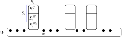
Figure 6: A bucket partition

Definition 7 (Bucket partition of a nice pair).

Let $f$ be a function from $\mathbb{N}$ to $\mathbb{R}^{+}$ and $\psi=(W,B)$ be a nice pair. Let $B^{C}=B\cap C^{0},$ and $B^{W}=B\cap W^{0}.$ For any $i\in S^{\psi},$ let $B_{i}^{C}=B_{i}\cap B^{C}.$ For any partition $(B^{W_{1}},B^{W_{2}})$ of $B^{W}$ and any $i\in S^{\psi},$ let $B_{i}^{W_{1}}=B_{i}\cap B^{W_{1}},$ $B_{i}^{W_{2}}=B_{i}\cap B^{W_{2}}$ and let $S_{i}=B_{i}^{C}\cup B_{i}^{W_{1}}.$

A bucket partition of a nice pair $\psi=(W,B)$ is a partition $(B^{W_{1}},B^{W_{2}})$ of $B^{W}$ such that

1. for any $i\in S^{\psi},$ $|S_{i}|\geq 1$

2. $|B^{W_{1}}|\leq 10|B^{C}|.$

We say that a bucket partition has local size $f$ if for any $i\in S^{\psi},$ $|B_{i}^{W_{2}}|\leq f(|S_{i}|).$

Notice that the size condition $|B^{W_{1}}|\leq 10|B^{C}|$ required in the bucket partition is a “global” constraint on the size of the $B^{W_{1}},$ while the condition size $|B_{i}^{W_{2}}|\leq f(|S_{i}|)$ required by the local size function is a “local” constraint on every bucket. We introduced this local notion of size as a way to control more precisely the number of vertices added to $B$ (and thus to the kernel output), which will be critical when typically adjacent buckets are merged using the add operation o Definition 14. However, when the kernel will find a rainbow matching and stop, the only role of these local sizes will be to upper bound the total size of $B$.

The object that our kernel will manipulate is a partial decomposition, as defined below.

Definition 8 (Partial decomposition).

We say that a tuple $(W,B,C,B^{W_{1}},B^{W_{2}})$ is a partial decomposition if

1. there is a partition $V({T})=W\cup B\cup C$

2. $C\subseteq C^{0}$

3. $(W,B)$ is a nice pair

4. $(B^{W_{1}},B^{W_{2}})$ is a bucket partition of $(W,B)$

We say that a partial decomposition has local size $f$ if $(B^{W_{1}},B^{W_{2}})$ has local size $f.$
Moreover, we will say that a partial decomposition is clean if it satisfies the following extra condition:

1. for every vertex $c\in C$ the tournament $T[W\cup\{c\}]$ contains a triangle.

Here again, we have a simple process, called the cleaning phase, to obtain a clean partial decomposition from any partial decomposition.

Lemma 11 (Cleaning Lemma).

Let $(W,B,C,B^{W_{1}},B^{W_{2}})$ be a partial decomposition and $X$ be set the of vertices $x$ of $C$ such that $T[W\cup\{x\}]$ does not contain any triangle. Then $(W,B\cup X,C\setminus X,B^{W_{1}},B^{W_{2}})$ is a clean partial decomposition of $T$, with the same local size than $(W,B,C,B^{W_{1}},B^{W_{2}})$.

Proof.

Let us first check that $(W,B\cup X,C\setminus X,B^{W_{1}},B^{W_{2}})$ satisfies the requirements of a partial decomposition. Properties 1 and 2 are clearly satisfy, and by choice of $X$, no vertex of $X$ is contained in a triangle with two vertices of $W$, so $\psi^{\prime}=(W,B\cup X)$ is also a nice pair and property 3 is satisfies. Notice that vertices of $X$ can create new buckets or be added in existing buckets of $\psi$, but in all cases we have $S^{\psi}\subseteq S^{\psi^{\prime}}$. Finally, in the buckets partition of $\psi^{\prime}$, the vertices of $X$ will be added to $B^{C}$. That is, with the notations of Definition 7, we have $(B\cup X)^{W}=B^{W}$, $(B\cup X)_{i}^{W_{j}}=B_{i}^{W_{j}}$ for $i\in S^{\psi}$ and $j=1,2$ and $(B\cup X)_{i}^{W_{j}}=\emptyset$ for $i\in S^{\psi^{\prime}}\setminus S^{\psi}$ and $j=1,2$. It is then straightforward to check that Properties 1. and 2., as well as the local size requirement, from Definition 7 still hold for $\psi^{\prime}$. In all, we can conclude that $(W,B\cup X,C\setminus X,B^{W_{1}},B^{W_{2}})$ is a clean partial decomposition with the same local size than $(W,B,C,B^{W_{1}},B^{W_{2}})$. ∎

6.4 Intervals: demand definition and basic properties

In this section we introduce the notion of demand for a partial decomposition. Informally, a demand is a set of bucket intervals with a value attached to each interval. The value $\textsf{val}(I)$ attached to interval $I$ depends on the contents of the buckets $\{B_{i}\mid i\in B(I)\}$ contained in $I$.

The notion of demand will be used in Subsection 6.6 to define the auxiliary edge-colored multigraph necessary in our approach. In particular, given a $\sqsubseteq$-minimal interval $I$ (implying that buckets $B_{l_{I}}$ and $B_{r_{I}}$ are consecutive), it will be important that $\textsf{val}(I)$ upper bounds the size of packing $\mathcal{P}$ where all triangles in $\mathcal{P}$ have one vertex in $B_{l_{I}}$, one in $B_{r_{I}}$, and one in $W(I)$. Indeed, $\textsf{val}(I)$ will correspond to the number of vertices that we want to find in $W(I)$ in the rainbow matching we look for. Then, if we indeed find such a rainbow matching, and thus a set $Q_{I}\subseteq W(I)$ with $|Q_{I}|=\textsf{val}(I)$, we must be able to repack such a packing $\mathcal{P}$ (corresponding to a part of an optimal solution) into a packing $\mathcal{P}^{\prime}$ of same size with $V(\mathcal{P}^{\prime})\subseteq B_{l_{I}}\cup B_{r_{I}}\cup Q_{I}$ by changing vertices used in $W(I)$ to take instead vertices in $Q_{I}$.

The following definition is illustrated Figure 7.

Definition 9 (Block partition).

We call a set $\mathcal{I}^{\textrm{max}}\subseteq\mathcal{BI}(\psi)$ proper if there do not exist $I_{1},I_{2}\in\mathcal{I}^{\textrm{max}}$ such that $I_{1}\neq I_{2}$ and $I_{1}\sqsubseteq I_{2}.$

Given a proper set $\mathcal{I}^{\textrm{max}}\subseteq\mathcal{BI}(\psi)$ of bucket intervals we define the block partition of $\mathcal{I}^{\textrm{max}},$ denoted $\{Z_{1},\dots,Z_{t}\},$ as follows. Let us order $\mathcal{I}^{\textrm{max}}$ according to the left points, meaning that $\mathcal{I}^{\textrm{max}}=\{I_{1},\dots,I_{x}\},$ where $l_{i}<l_{i+1}$ (and $r_{i}<r_{i+1}$) for any $i.$

We find the largest $x_{1}$ such that $I_{1}\prec I_{2}\prec\dots\prec I_{x_{1}}$ and define $Z_{1}=\{I_{i}\mid x_{0}+1\leq i\leq x_{1}\}$ where $x_{0}=0.$ Then, we find the largest $x_{2}$ such that $I_{x_{1}+1}\prec I_{x_{1}+2}\prec\dots\prec I_{x_{2}},$ and define $Z_{2}=\{I_{i}\mid x_{1}+1\leq i\leq x_{2}\}.$ We continue until we have a partition $\{Z_{\ell},\ell\in[t]\}$ of $\mathcal{I}^{\textrm{max}}$ (implying $x_{t}=x$).

Notice that, for any $\ell\in[t-1],$ $I_{x_{l}}\nprec I_{x_{l}+1},$ implying that $r_{I_{x_{l}}}\leq l_{I_{x_{l}+1}}.$ We also define the block intervals as $I^{*}_{\ell}=\sqcup_{I\in Z_{\ell}}I$ for any $\ell\in[t].$

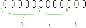
Figure 7: A block partition of $\mathcal{I}^{\textrm{max}}=\{I_{1},\dots,I_{6}\}.$ We have $Z_{1}=\{I_{1},I_{2},I_{3}\},$ $Z_{2}=\{I_{4},I_{5}\}$ and $Z_{3}=\{I_{6}\}.$

The next lemma follows from the previous definition.

Lemma 12.

Let $\psi$ be a nice pair, $\mathcal{J}\subseteq\mathcal{BI}(\psi)$ a set of bucket intervals, and let $\mathcal{J}^{\textrm{max}}\subseteq\mathcal{J}$ be the subset of $\sqsubseteq$-wise maximal bucket intervals of $\mathcal{J}.$ Let $\{Z_{\ell},\ell\in[t]\}$ and $\{I^{*}_{\ell},\ell\in[t]\}$ be the block partition and block intervals of $\mathcal{J}^{\textrm{max}}$ (which is well defined as $\mathcal{J}^{\textrm{max}}$ is proper). Then, we have $\mathcal{J}=\bigcup_{\ell\in[t]}\mathcal{P}_{\mathcal{J}}(I^{*}_{\ell})$

Proof.

Indeed, we have the following.

$$\mathcal{J}=\bigcup_{I\in\mathcal{J}^{\textrm{max}}}P_{\mathcal{J}}(I)=\bigcup_{\ell\in[t]}\bigcup_{I\in Z_{\ell}}P_{\mathcal{J}}(I)=\bigcup_{\ell\in[t]}\mathcal{P}_{\mathcal{J}}(I^{*}_{\ell})$$

∎

The two next definitions introduce the notion of demand for a partial decomposition of a nice pair and are illustrated in Figure 8.

Definition 10.

Let $(W,B,C,B^{W_{1}},B^{W_{2}})$ be a partial decomposition and $I$ a bucket interval. We define

• $\Sigma(I)=\sum_{i\in B(I)}|S_{i}|$

• $m(I)=\sum_{i\in B(I)}|B_{i}|-|B_{i_{0}}|$ where $i_{0}\in\textrm{ argmax}_{i\in B(I)}|B(i)|$

• $\mu(I)=\min\big{\{}\Sigma(I),m(I)\big{\}}$

• $t(I)=\begin{cases}\text{\tt{\Sigma}}&\text{if }\Sigma(I)<m(I)\\ \text{\tt{m}}&\text{if }\Sigma(I)>m(I)\\ \text{\tt{=}}&\text{otherwise.}\end{cases}$

Interval	$I_{1}$	$I_{2}$	$I_{3}$	$I_{4}$	$I_{5}$	$I_{6}$
Bounds	$[1,2]$	$[2,3]$	$[3,4]$	$[1,3]$	$[2,4]$	$[1,4]$
$\Sigma$	5	2	11	6	12	16
$m$	3	3	5	8	8	15
$\mu$	3	2	5	6	8	15
$t$	m	Σ	m	Σ	m	m

Figure 8: Example of a demand $(\mathcal{I},\textsf{val}).$ On the left, the buckets are depicted and the cardinalities of $S_{1}$ and $B_{1}^{W_{2}}$ are indicated. Below, stand the intervals with their value. On the right, for every interval, the values $\Sigma,$ $m,$ $\mu$ and $t$ are computed.

To get an insight on why we used the previous definition of $\mu$, one can check that the property announced at the begining of this section holds: let us consider a $\sqsubseteq$-minimal interval $I$ (implying that buckets $B_{l_{I}}$ and $B_{r_{I}}$ are consecutive), and check that $\textsf{val}(I)$ upper bounds the size of packing $\mathcal{P}$ where all triangles in $\mathcal{P}$ have one vertex in $B_{l_{I}}$, one in $B_{r_{I}}$, and one in $W(I)$. On one hand, as any such triangle consumes one vertex in $B_{l_{I}}$ and one in $B_{r_{I}}$, we get $|\mathcal{P}|\leq\min(|B_{l_{I}}|,|B_{r_{I}}|)=m(I)$. On the other hand, as any triangle in $\mathcal{P}$ cannot use only vertices in $W^{0}$, it must uses at least one vertex from $S_{l_{I}}\cup S_{r_{I}}$, implying that $|\mathcal{P}|\leq\text{\tt{\Sigma}}(I)$. We discuss at the end of Subsection 6.7 why taking simply $\mu(I)=\text{\tt{\Sigma}}(I)$ or $\mu(I)=m(I)$ would not be sufficient to get a kernel in $\mathcal{O}(k^{\delta})$ for any $\delta>1$.

Definition 11 (Demand).

Let $(W,B,C,B^{W_{1}},B^{W_{2}})$ be a partial decomposition of $\psi.$ Let us define the following polynomial algorithm which, given $(W,B,C,B^{W_{1}},B^{W_{2}}),$ computes a set $\mathcal{I}$ of bucket intervals of $\psi,$ and a value $\textsf{val}(I)$ for any $I\in\mathcal{I}.$

• start with $X=\emptyset$

• for any $L\in[2,|S^{\psi}|]$ do

  • for any bucket interval $I$ of $\psi$ where $|B(I)|=L$:

  • let $\textsf{val}(P_{X}(I))=\sum_{I\in P_{X}(I)}\textsf{val}(I).$ Notice that at this stage $I\notin P_{X}(I),$ and in particular we have $\textsf{val}(P_{X}(I))=0$ if $L=2.$

  • if $\textsf{val}(P_{X}(I))\leq\mu(I)$ then define $\textsf{val}(I)=\mu(I)-\textsf{val}(P_{X}(I)),$ and add $I$ to $X$ (and thus, in this case, $I\in P_{X}(I)$)

• let $\mathcal{I}=X$

• return $(\mathcal{I},\textsf{val})$

We call the pair $(\mathcal{I},\textsf{val})$ the demand for $(W,B,C,B^{W_{1}},B^{W_{2}})$. We denote

$$\mathcal{I}_{>0}=\{I\in\mathcal{I}\mid\textsf{val}(I)>0\}.$$

For any $X\subseteq\mathcal{I},$ we also denote $\textsf{val}(X)=\sum_{I\in X}\textsf{val}(I).$

Observe that in the example of Figure 8 we have $\mathcal{I}_{>0}=\mathcal{I}=\mathcal{BI},$ but it may be the case that $\mathcal{I}_{>0}\subsetneq\mathcal{I}\subsetneq\mathcal{BI}.$ Let us now provide properties on demands.

Lemma 13.

Let $(W,B,C,B^{W_{1}},B^{W_{2}})$ be a partial decomposition and $(\mathcal{I},\textsf{val})$ be its demand. Then, for any $I\in\mathcal{BI}(W,B)$:

1. $\textsf{val}(P_{\mathcal{I}}(I))=\textsf{val}(P_{\mathcal{I}_{>0}}(I))$

2. $\textsf{val}(P_{\mathcal{I}}(I))\geq\mu(I)$

3. $I\in\mathcal{I}\Leftrightarrow\textsf{val}(P_{\mathcal{I}}(I))=\mu(I)\Leftrightarrow\textsf{val}(P_{\mathcal{I}}(I)\setminus\{I\})\leq\mu(I)$

4. $I\in\mathcal{I}_{>0}\Leftrightarrow\textsf{val}(P_{\mathcal{I}}(I)\setminus\{I\})<\mu(I)$

5. if $t(I)=\text{\tt{\Sigma}},$ then for any $i_{0}\in\textrm{ argmax}_{i\in B(I)}|B(i)|,$ we have $|S_{i_{0}}|<\sum_{i\in B(I)\setminus\{i_{0}\}}|B_{i}^{W_{2}}|$

6. if there exists $i_{0}\in\textrm{ argmax}_{i\in B(I)}|B(i)|$ such that $|S_{i_{0}}|<\sum_{i\in B(I)\setminus\{i_{0}\}}|B_{i}^{W_{2}}|,$ then we have $t(I)=\text{\tt{\Sigma}}$

7. if $t(I)=\text{\tt{m}},$ then for any $i_{0}\in\textrm{ argmax}_{i\in B(I)}|B(i)|,$ we have $|S_{i_{0}}|>\sum_{i\in B(I)\setminus\{i_{0}\}}|B_{i}^{W_{2}}|$

Before proving Lemma 13, notice that for every interval $I$ in Figure 8, computing its demand leads to $I\in\mathcal{I}$ and $\textsf{val}(P_{\mathcal{I}}(I))=\mu(I),$ illustrating Property 3 above.

Proof.

Let $I\in\mathcal{BI}(W,B).$ In what follows, we consider the iteration where the algorithm considers $I,$ and let $X$ denote the variable of the algorithm at the line where it computes $\textsf{val}(P_{X}(I)).$ Observe first that, no matter whether the algorithm decides to add $I$ in $X$ or not, we have $P_{X}(I)=P_{\mathcal{I}}(I)\setminus\{I\}.$ In particular, we have the following equivalences :

• $I\notin\mathcal{I}$ $\Leftrightarrow P_{\mathcal{I}}(I)=P_{X}(I)\Leftrightarrow\textsf{val}(P_{X}(I))>\mu(I).$

• $I\in\mathcal{I}$ $\Leftrightarrow P_{\mathcal{I}}(I)=P_{X}(I)\cup\{I\}\Leftrightarrow\textsf{val}(P_{X}(I))\leq\mu(I)$ .

Now, we can prove Properties 1 to 7.

Property $\mathbf{1}$ is immediate.

Property $\mathbf{2}$ holds in the case where $I\notin\mathcal{I}.$ In case $I\in\mathcal{I},$ we have $\textsf{val}(P_{\mathcal{I}}(I))=\textsf{val}(P_{X}(I))+\textsf{val}(I)=\mu(I)$ and the property holds.

The first equivalence of Property 3 follows from the proof of Property 2 above. As $\textsf{val}(P_{X}(I))=\textsf{val}(P_{\mathcal{I}}(I)\setminus\{I\}),$ we get the second part of Property $\mathbf{3}$ from the seminal observation.

Property $\mathbf{4}$ can be rewritten as $I\in\mathcal{I}_{>0}\Leftrightarrow\textsf{val}(P_{X}(I))<\mu(I).$ Since $\mathcal{I}\in\mathcal{I}\Leftrightarrow\textsf{val}(I)=\mu(I)-P_{X}(\mathcal{I}),$ we get $\textsf{val}(I)>0\Leftrightarrow\textsf{val}(P_{X}(I))<\mu(I),$ implying Property $\mathbf{4}.$

For Properties $\mathbf{5}$ and $\mathbf{6},$ let $i_{0}\in\textrm{ argmax}_{i\in B(I)}|B(i)|.$

$$t(I)=\text{\tt{\Sigma}} \Leftrightarrow \sum_{i\in B(I)}|S_{i}|<\sum_{i\in B(I)\setminus\{i_{0}\}}|B_{i}|$$

$$\Leftrightarrow \sum_{i\in B(I)}|S_{i}|<\sum_{i\in B(I)\setminus\{i_{0}\}}(|S_{i}|+|B^{W_{2}}_{i}|)$$

$$\Leftrightarrow |S_{i_{0}}|<\sum_{i\in B(I)\setminus\{i_{0}\}}|B^{W_{2}}_{i}|$$

Property $\mathbf{7}$ is obtained by reversing the above inequalities. ∎

6.5 The small total demand property

The objective of the section is only to prove Lemma 16. To that end, we prove that the “intersection property” of Lemma 14 implies the “union property” of Lemma 15, which finally implies Lemma 16.

Lemma 14 (The intersection property).

Let $(W,B,C,B^{W_{1}},B^{W_{2}})$ be a partial decomposition and $(\mathcal{I},\textsf{val})$ be its demand. Let $I_{1},I_{2}$ in $\mathcal{I}_{>0}$ such that $I_{1}\prec I_{2}.$ Then, $t(I_{1}\sqcap I_{2})=\text{\tt{\Sigma}}.$

An example of the intersection property can be seen in Figure 8 where $t(I_{4}\sqcap I_{5})=t(I_{2})=\text{\tt{\Sigma}}.$

Proof.

We refer the reader to Figure 9 for an illustration of the notations used in this proof.

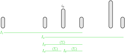
Figure 9: Notations for the intersection property proof.

Let $I_{3}=I_{1}\sqcap I_{2},$ and observe that $I_{3}=[l_{I_{2}},r_{I_{1}}].$ Let $i_{0}\in\textrm{ argmax}_{i\in B(I_{3})}|B_{i}|.$ Let $I_{a}=(l_{I_{2}},i_{0})$ and $I_{b}=(i_{0},r_{I_{1}}).$ Observe that $I_{a}$ or $I_{b}$ may not be a bucket interval (when $i_{0}=l_{I_{2}}$ or $i_{0}=r_{I_{1}}$), but at least one of them is a bucket interval. Let $X=\{I_{a},I_{b}\}\cap\mathcal{BI}.$

We now show that, for any $I\in X,$ $t(I)=\text{\tt{\Sigma}}.$ Without loss of generality, assume $I_{a}\in X,$ which implies $l_{I_{2}}<i_{0}.$ Suppose, towards a contradiction, that $t(I_{a})\in\{\text{\tt{=}},\text{\tt{m}}\}.$ Observe that $i_{0}\in\textrm{ argmax}_{i\in B(I_{a})}|B_{i}|,$ implying $\mu(I_{a})=\sum_{i\in B(I_{a})}|B_{i}|-|B_{i_{0}}|.$ Let $I_{a^{\prime}}=(i_{0},r_{I_{2}}).$ Observe that $I_{a^{\prime}}$ is a bucket interval as $i_{0}\leq r_{I_{1}}<r_{I_{2}}$ (as we have $I_{1}\prec I_{2}$). Note that $P_{\mathcal{I}}(I_{a})\cap P_{\mathcal{I}}(I_{a^{\prime}})=\emptyset,$ $P_{\mathcal{I}}(I_{a})\subseteq P_{\mathcal{I}}(I_{2})\setminus\{I_{2}\},$ and $P_{\mathcal{I}}(I_{a^{\prime}})\subseteq P_{\mathcal{I}}(I_{2})\setminus\{I_{2}\}.$ By combining these observations, we obtain

$$\textsf{val}(P_{\mathcal{I}}(I_{2})\setminus\{I_{2}\}) \geq \textsf{val}(P_{\mathcal{I}}(I_{a}))+\textsf{val}(P_{\mathcal{I}}(I_{a^{\prime}}))$$

$$\geq \mu(I_{a})+\mu(I_{a^{\prime}})\mbox{ by Lemma\leavevmode\nobreak\ \ref{@personalmente} Property {\bf 2}}$$

Let us now prove that $\mu(I_{a})+\mu(I_{a^{\prime}})\geq\mu(I_{2}).$ This will imply $\textsf{val}(P_{\mathcal{I}}(I_{2})\setminus\{I_{2}\})\geq\mu(I_{2}),$ which contradicts Lemma 13 Property 4 as $\textsf{val}(I_{2})>0.$

We now distinguish two cases according to $t(I_{a^{\prime}}).$

Case 1: $t(I_{a^{\prime}})\in\{\text{\tt{\Sigma}},\text{\tt{=}}\}.$
In this case, $\mu(I_{a^{\prime}})=\sum_{i\in B(I_{a^{\prime}})}|S_{i}|$ and we have the following.

$$\mu(I_{a})+\mu(I_{a^{\prime}}) = \sum_{i\in B(I_{a})}|B_{i}|-|B_{i_{0}}|+\sum_{i\in B(I_{a^{\prime}})}|S_{i}|$$

$$= \sum_{i\in B(I_{a})\setminus\{i_{0}\}}|B_{i}|+\sum_{i\in B(I_{a^{\prime}})}|S_{i}|$$

$$\geq \sum_{i\in B(I_{a})\setminus\{i_{0}\}}|S_{i}|+\sum_{i\in B(I_{a^{\prime}})}|S_{i}|$$

$$\geq \Sigma(I_{2})$$

$$\geq \mu(I_{2})$$

Case 2: $t(I_{a^{\prime}})=\text{\tt{m}}.$
In this case, $\mu(I_{a^{\prime}})=\sum_{i\in B(I_{a^{\prime}})}|B_{i}|-|B_{i_{1}}|,$ where $i_{1}\in\textrm{ argmax}_{i\in B(I_{a^{\prime}})}|B_{i}|.$ Notice that $|B_{i_{1}}|\geq|B_{i_{0}}|.$ Let $i_{2}\in\textrm{ argmax}_{i\in B(I_{2})}|B_{i}|.$ Observe that $|B_{i_{2}}|=|B_{i_{1}}|,$ and that in the two cases ($i_{1}=i_{0}$ or $i_{1}\neq i_{0}$) we have $\mu(I_{a})+\mu(I_{a^{\prime}})=\sum_{i\in B(I_{2})}|B_{i}|-|B_{i_{1}}|=m(I_{2})\geq\mu(I_{2}).$ This concludes the proof of our claim, and we now assume that for any $I\in X,$ $t(I)=\text{\tt{\Sigma}}.$

Let us now prove that $t(I_{3})=\text{\tt{\Sigma}}.$ If $i_{0}=l_{I_{2}}$ or $i_{0}=r_{I_{1}},$ then $X=\{I_{3}\},$ and we are done. Suppose now $l_{I_{2}}<i_{0}<r_{I_{1}}.$ Observe that $i_{0}\in\textrm{ argmax}_{i\in B(I_{3})}|B_{i}|$ implies $i_{0}\in\textrm{ argmax}_{i\in B(I_{a})}|B_{i}|.$ As $t(I_{a})=\text{\tt{\Sigma}}$ and as $i_{0}\in\textrm{ argmax}_{i\in B(I_{a})}|B_{i}|,$ Lemma 13 Property 5 implies $|S_{i_{0}}|<\sum_{i\in B(I_{a})\setminus\{i_{0}\}}|B_{i}^{W_{2}}|\leq\sum_{i\in B(I_{3})\setminus\{i_{0}\}}|B_{i}^{W_{2}}|.$ By Lemma 13 Property 6, this implies $t(I_{3})=\text{\tt{\Sigma}}.$ ∎

Lemma 15 (The union property).

Let $(W,B,C,B^{W_{1}},B^{W_{2}})$ be a partial decomposition and $(\mathcal{I},\textsf{val})$ be its demand. Let $\mathcal{Z}\subseteq\mathcal{I}_{>0},$ where $\mathcal{Z}=\{I_{1},\dots,I_{x}\}$ for some $x\geq 1,$ and where $I_{i}\prec I_{i+1}$ for any $i=1,\dots,x-1.$ Then, we have $\sqcup_{I\in{\mathcal{Z}}}I\in\mathcal{I}.$

Proof.

We refer the reader to Figure 10 for notations.

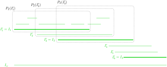
Figure 10: Interval of $\mathcal{Z}$ are represented in bold.

Let $I_{\sqcup}=\sqcup_{I\in Z}I.$ Let also

$${\mathcal{Z}^{\textrm{max}}}=\{I\in\mathcal{I}_{>0}\mid I\subseteq I_{\sqcup},I\neq I_{\sqcup}\mbox{ and $I$ is $\sqsubseteq$-wise maximal}\}.$$

Let $\mathcal{Z}^{\textrm{max}}=\{I^{\prime}_{1},\dots,I^{\prime}_{y}\},$ where intervals are ordered according to their left endpoint. If $x=1,$ the lemma follows immediately, and thus we may assume $x\geq 2$ which implies $y\geq 2$ as well.

Let us prove that we even have $I^{\prime}_{i}\prec I^{\prime}_{i+1},$ for any $i.$ Let $i\in[y-1]$ and let $j_{0}$ be the minimum $j$ such that $r_{I^{\prime}_{i}}<r_{I_{j}}.$ Such a $j_{0}$ exists, as $i\leq y-1,$ and thus $r_{I^{\prime}_{i}}<r(I_{\sqcup}).$ Moreover, $j_{0}>1$ as otherwise we would have $I^{\prime}_{i}\sqsubset I_{j_{0}},$ a contradiction to the fact that $I^{\prime}_{i}$ is $\sqsubseteq$-wise maximal. Notice first that $I_{j_{0}}\nsubseteq I^{\prime}_{\ell},$ for any $\ell\leq i.$ As $I_{j_{0}-1}\prec I_{j_{0}},$ we get $l_{I_{j_{0}}}<r_{I_{j_{0}-1}}$ and, moreover, by the definition of $j_{0},$ we get $r_{I_{j_{0}-1}}\leq r_{I^{\prime}_{i}},$ implying $l_{I_{j_{0}}}<r_{I^{\prime}_{i}}.$ Thus, if, towards a contradiction, we do not have $I_{i}^{\prime}\prec I_{i+1}^{\prime}$ then we had $r_{I^{\prime}_{i}}\leq l_{I^{\prime}_{i+1}}$ and we would have $l_{I_{j_{0}}}<l_{I^{\prime}_{i+1}},$ implying that $I_{j_{0}}\nsubseteq I^{\prime}_{\ell}$ for any $\ell\geq i+1.$ Thus, there would be no $I\in\mathcal{Z}^{\textrm{max}}$ such that $I_{j_{0}}\sqsubseteq I,$ which is a contradiction as $I_{j_{0}}\neq I_{\sqcup}.$ This concludes the proof that $I^{\prime}_{i}\prec I^{\prime}_{i+1},$ for any $i.$

According to Lemma 13, $I_{\sqcup}\in\mathcal{I}\Leftrightarrow\textsf{val}(P_{\mathcal{I}}(I_{\sqcup})\setminus\{I_{\sqcup}\})\leq\mu(I_{\sqcup}),$ and thus our objective is to prove that $\textsf{val}(P_{\mathcal{I}}(I_{\sqcup})\setminus\{I_{\sqcup}\})\leq\mu(I_{\sqcup}).$

By definition of $\mathcal{Z}^{\textrm{max}},$ we get $P_{\mathcal{I}}(I_{\sqcup})\setminus\{I_{\sqcup}\}=\bigcup_{\ell\in[y]}P_{\mathcal{I}}(I^{\prime}_{\ell})$ (see Figure 10). Thus, $\textsf{val}(P_{\mathcal{I}}(I_{\sqcup})\setminus\{I_{\sqcup}\})=\textsf{val}(\bigcup_{\ell\in[y]}P_{\mathcal{I}}(I^{\prime}_{\ell})).$ Let us now prove that $\textsf{val}(\bigcup_{\ell\in[y]}P_{\mathcal{I}}(I^{\prime}_{\ell}))=s,$ where

$$s=\sum_{\ell\in[y]}\textsf{val}(P_{\mathcal{I}}(I^{\prime}_{\ell}))-\sum_{\ell\in[y-1]}\textsf{val}(P_{\mathcal{I}}(I^{\prime}_{\ell})\cap P_{\mathcal{I}}(I^{\prime}_{\ell+1})).$$

Let $I\in\bigcup_{\ell\in[y]}P_{\mathcal{I}}(I^{\prime}_{\ell})$ and let us prove that $\textsf{val}(I)$ appears exactly one time in $s.$ Let $\ell_{1}$ (resp. $\ell_{2}$) the minimum (resp. maximum) value such that $I\in\mathcal{P}_{I}(I^{\prime}_{\ell}).$ Observe that $\textsf{val}(I)$ appears $\ell_{2}-\ell_{1}+1$ times in $\sum_{\ell\in[y]}\textsf{val}(P_{\mathcal{I}}(I^{\prime}_{\ell})),$ and $\ell_{2}-\ell_{1}$ times in $\sum_{\ell\in[y-1]}\textsf{val}(P_{\mathcal{I}}(I^{\prime}_{\ell})\cap P_{\mathcal{I}}(I^{\prime}_{\ell+1})),$ and thus exactly $1$ time in $s.$ Moreover, as for any $\ell\in[y-1],$ $P_{\mathcal{I}}(I^{\prime}_{\ell})\cap P_{\mathcal{I}}(I^{\prime}_{\ell+1})=P_{\mathcal{I}}(I^{\prime}_{\ell}\cap I^{\prime}_{\ell+1}),$ we can even rewrite

$$s=\sum_{\ell\in[y]}\textsf{val}(P_{\mathcal{I}}(I^{\prime}_{\ell}))-\sum_{\ell\in[y-1]}\textsf{val}(P_{\mathcal{I}}(I^{\prime}_{\ell}\cap I^{\prime}_{\ell+1})).$$

It now remains to prove that $s\leq\mu(I_{\sqcup}).$

$$s = \sum_{\ell\in[y]}\textsf{val}(P_{\mathcal{I}}(I^{\prime}_{\ell}))-\sum_{\ell\in[y-1]}\textsf{val}(P_{\mathcal{I}}(I^{\prime}_{\ell}\cap I^{\prime}_{\ell+1}))$$

$$= \sum_{\ell\in[y]}\mu(I^{\prime}_{\ell})-\sum_{\ell\in[y-1]}\textsf{val}(P_{\mathcal{I}}(I^{\prime}_{\ell}\cap I^{\prime}_{\ell+1})),\mbox{ by Lemma\leavevmode\nobreak\ \ref{@personalmente} Property {\bf 3} as $I^{\prime}_{\ell}\in\mathcal{I}$}$$

$$\leq \sum_{\ell\in[y]}\mu(I^{\prime}_{\ell})-\sum_{\ell\in[y-1]}\mu(I^{\prime}_{\ell}\cap I^{\prime}_{\ell+1}),\mbox{ by Lemma\leavevmode\nobreak\ \ref{@personalmente} Property {\bf 2}}$$

$$\leq \sum_{\ell\in[y]}\mu(I^{\prime}_{\ell})-\sum_{\ell\in[y-1]}\sum_{i\in B(I^{\prime}_{\ell}\cap I^{\prime}_{\ell+1})}|S_{i}|,\mbox{ by Lemma\leavevmode\nobreak\ \ref{lemma_intersection} and as we have }I_{\ell}^{\prime}\in\mathcal{I}_{>0}\mbox{ for all }\ell\in[y]$$

Let us now distinguish two cases according to $t(I_{\sqcup}).$

Case 1: $t(I_{\sqcup})\in\{\text{\tt{\Sigma}},\text{\tt{=}}\}.$
In this case, $\mu(I_{\sqcup})=\sum_{i\in B(I_{\sqcup})}|S_{i}|,$ and we have the following.

$$s \leq \sum_{\ell\in[y]}\sum_{i\in B(I^{\prime}_{\ell})}|S_{i}|-\sum_{\ell\in[y-1]}\sum_{i\in B(I^{\prime}_{\ell}\cap I^{\prime}_{\ell+1})}|S_{i}|,\mbox{ by definition of $\mu$}$$

$$= \sum_{i\in B(\bigcup_{\ell\in[y]}I^{\prime}_{l})}|S_{i}|,\mbox{ as for any $i,$ the term $|S_{i}|$ appears exactly once}$$

$$= \Sigma(I_{\sqcup})$$

$$\leq \mu(I_{\sqcup})\mbox{ as we are in case 1}$$

Case 2: $t(I_{\sqcup})=\text{\tt{m}}.$
Let $i_{0}\in\textrm{ argmax}_{i\in B(I_{\sqcup})}|B_{i}|.$ In this case, $\mu(I_{\sqcup})=\sum_{i\in B(I_{\sqcup})}|B_{i}|-|B_{i_{0}}|,$ and according to Lemma 13 Property 7, we have $|S_{i_{0}}|>\sum_{i\in B(I_{\sqcup})\setminus\{i_{0}\}}|B_{i}^{W_{2}}|.$

Let us prove the following property: Let $B^{*}=\Big{(}B(I^{\prime}_{1})\setminus\bigcup_{2\leq\ell\leq y}B(I^{\prime}_{\ell})\Big{)}\cup\Big{(}B(I^{\prime}_{y})\setminus\bigcup_{1\leq\ell\leq y-1}B(I^{\prime}_{\ell})\Big{)},$ then $i_{0}\in B^{*}.$ This property means that $i_{0}$ is in one of the two “extreme” sides of the union. For example, in Figure 8, where $I^{\prime}_{1}=I_{4},I^{\prime}_{2}=I_{5},$ and $I_{\sqcup}=I_{6},$ we have that $t(I_{\sqcup})=\text{\tt{m}},$ $i_{0}=4,$ and $i_{0}\in B(I^{\prime}_{2})\setminus B(I^{\prime}_{1}).$

Observe that, as $I^{\prime}_{\ell}\prec I^{\prime}_{\ell+1}$ for any $\ell,$ it holds that, for all $i\in B(I_{\sqcup})\setminus B^{*},$ there exists $\ell$ such that $i\in B(I^{\prime}_{\ell})\cap B(I^{\prime}_{\ell+1}).$ Assume, towards a contradiction, that $i_{0}\notin B^{*},$ implying that there exists $\ell_{0}$ such that $i_{0}\in B(I^{\prime}_{\ell_{0}})\cap B(I^{\prime}_{\ell_{0}+1}).$ Therefore $i_{0}\in B(I^{\prime}_{\sqcap}),$ where $I^{\prime}_{\sqcap}=I^{\prime}_{\ell_{0}}\sqcap I^{\prime}_{\ell_{0}+1}.$ By Lemma 14, as $I^{\prime}_{\ell_{0}}$ and $I^{\prime}_{\ell_{0}}$ are in $\mathcal{I}_{>0}$ and $I^{\prime}_{\ell_{0}}\prec I^{\prime}_{\ell_{0}+1},$ we get $t(I^{\prime}_{\sqcap})=\text{\tt{\Sigma}}.$ By Lemma 13 Property 5, and as $i_{0}\in\textrm{ argmax}_{i\in B(I^{\prime}_{\sqcap})},$ we get $|S_{i_{0}}|<\sum_{i\in B(I^{\prime}_{\sqcap})\setminus\{i_{0}\}}|B_{i}^{W_{2}}|<\sum_{i\in B(I_{\sqcup})\setminus\{i_{0}\}}|B_{i}^{W_{2}}|,$ a contradiction.

Hence the property holds and, without loss of generality, we may assume $i_{0}\in B(I^{\prime}_{1})\setminus\bigcup_{2\leq\ell\leq y}B(I^{\prime}_{\ell}).$ Note that the case where $i_{0}\in B(I^{\prime}_{y})\setminus\bigcup_{1\leq\ell\leq y-1}B(I^{\prime}_{\ell})$ is symmetric.

Observe that $i_{0}\in\textrm{ argmax}_{i\in B(I^{\prime}_{1})}|B(i)|$ which implies $m(I^{\prime}_{1})=\sum_{i\in B(I^{\prime}_{1})\setminus\{i_{0}\}}|B_{i}|.$

As $i_{0}\in B(I^{\prime}_{1})\setminus\bigcup_{2\leq\ell\leq y}B(I^{\prime}_{\ell}),$ we have $i_{0}\in[l(I^{\prime}_{1}),l(I^{\prime}_{2})[,$ and thus

$$m(I^{\prime}_{1})=\sum_{i\in[l(I^{\prime}_{1}),l(I^{\prime}_{2})[\setminus\{i_{0}\}}|B_{i}|+\sum_{i\in[l(I^{\prime}_{2}),r(I^{\prime}_{1})]}(|S_{i}|+|B^{W_{2}}_{i}|).$$

We conclude that

$$s \leq \sum_{\ell\in[y]}\mu(I^{\prime}_{\ell})-\sum_{\ell\in[y-1]}\sum_{i\in B(I^{\prime}_{\ell}\cap I^{\prime}_{\ell+1})}|S_{i}|$$

$$\leq m(I^{\prime}_{1})+\sum_{2\leq\ell\leq y}\Sigma(I^{\prime}_{\ell})-\sum_{\ell\in[y-1]}\sum_{i\in B(I^{\prime}_{\ell}\cap I^{\prime}_{\ell+1})}|S_{i}|$$

$$= \sum_{i\in[l(I^{\prime}_{1}),l(I^{\prime}_{2})[\setminus\{i_{0}\}}|B_{i}|+\sum_{i\in[l(I^{\prime}_{2}),r(I^{\prime}_{1})]}(|S_{i}|+|B^{W_{2}}_{i}|)+$$

$$\leavevmode\nobreak\ \leavevmode\nobreak\ \leavevmode\nobreak\ \leavevmode\nobreak\ \leavevmode\nobreak\ \leavevmode\nobreak\ \leavevmode\nobreak\ \leavevmode\nobreak\ \leavevmode\nobreak\ \leavevmode\nobreak\ \leavevmode\nobreak\ \leavevmode\nobreak\ \leavevmode\nobreak\ \leavevmode\nobreak\ \leavevmode\nobreak\ \leavevmode\nobreak\ \leavevmode\nobreak\ \leavevmode\nobreak\ \leavevmode\nobreak\ \leavevmode\nobreak\ \leavevmode\nobreak\ \leavevmode\nobreak\ \leavevmode\nobreak\ \leavevmode\nobreak\ \leavevmode\nobreak\ \leavevmode\nobreak\ \leavevmode\nobreak\ \leavevmode\nobreak\ \leavevmode\nobreak\ \leavevmode\nobreak\ \leavevmode\nobreak\ \leavevmode\nobreak\ \leavevmode\nobreak\ \leavevmode\nobreak\ \leavevmode\nobreak\ \leavevmode\nobreak\ \leavevmode\nobreak\ \leavevmode\nobreak\ \leavevmode\nobreak\ \leavevmode\nobreak\ \leavevmode\nobreak\ \leavevmode\nobreak\ \leavevmode\nobreak\ \leavevmode\nobreak\ \leavevmode\nobreak\ \leavevmode\nobreak\ \leavevmode\nobreak\ \leavevmode\nobreak\ \leavevmode\nobreak\ \leavevmode\nobreak\ \leavevmode\nobreak\ \leavevmode\nobreak\ \leavevmode\nobreak\ \leavevmode\nobreak\ \leavevmode\nobreak\ \leavevmode\nobreak\ \sum_{2\leq\ell\leq y}\sum_{i\in B(I^{\prime}_{\ell})}|S_{i}|-\sum_{\ell\in[y-1]}\sum_{i\in B(I^{\prime}_{\ell}\cap I^{\prime}_{\ell+1})}|S_{i}|$$

$$= \sum_{i\in[l(I^{\prime}_{1}),l(I^{\prime}_{2})[\setminus\{i_{0}\}}|B_{i}|+\sum_{i\in[l(I^{\prime}_{2}),r(I^{\prime}_{1})]}|B^{W_{2}}_{i}|+\sum_{1\leq\ell\leq y}\sum_{i\in B(I^{*}_{\ell})}|S_{i}|-\sum_{\ell\in[y-1]}\sum_{i\in B(I^{*}_{\ell}\cap I^{*}_{\ell+1})}|S_{i}|$$

by defining $$I^{*}_{1}=[l(I^{\prime}_{2}),r(I^{\prime}_{1})] I^{*}_{\ell}=I^{\prime}_{\ell}, 2\leq\ell\leq y$$ and for any

$$= \sum_{i\in[l(I^{\prime}_{1}),l(I^{\prime}_{2})[\setminus\{i_{0}\}}|B_{i}|+\sum_{i\in[l(I^{\prime}_{2}),r(I^{\prime}_{1})]}|B^{W_{2}}_{i}|+\sum_{i\in B(\bigcup_{\ell\in[y]}I^{*}_{l})}|S_{i}|$$

as, for any $$i, |S_{i}|$$ each term appears exactly once

$$= \sum_{i\in B(I^{\prime}_{1})\setminus\{i_{0}\}}|B_{i}|+\sum_{i\in B(I_{\sqcup})\setminus B(I^{\prime}_{1})}|S_{i}|$$

$$\leq \sum_{i\in B(I^{\prime}_{1})\setminus\{i_{0}\}}|B_{i}|+\sum_{i\in B(I_{\sqcup})\setminus B(I^{\prime}_{1})}|B_{i}|$$

$$= m(I_{\sqcup})$$

$$\leq \mu(I_{\sqcup}),\mbox{ as we are in Case 2.}$$

∎

The following lemma will be used in both cases of our kernelization algorithm (rainbow matching or small vertex cover) in order to prove that what is added in the kernel is small.

Lemma 16 (The small total demand property).

Let $(W,B,C,B^{W_{1}},B^{W_{2}})$ be a partial decomposition and $(\mathcal{I},\textsf{val})$ be its demand. Let $\mathcal{J}\subseteq\mathcal{I}_{>0},$ and let $\mathcal{J}^{\textrm{max}}\subseteq\mathcal{J}$ be the subset of $\sqsubseteq$-wise maximal bucket intervals of $\mathcal{J}.$ Let $\{Z_{\ell},\ell\in[t]\}$ and $\{I^{*}_{\ell},\ell\in[t]\}$ be the block partition and block intervals of $\mathcal{J}^{\textrm{max}}.$ Then, we have $\textsf{val}(\mathcal{J})\leq\sum_{\ell\in[t]}\mu(I^{*}_{\ell}).$

Proof.

According to Lemma 12 we have, $\mathcal{J}=\bigcup_{\ell\in[t]}\mathcal{P}_{\mathcal{J}}(I^{*}_{\ell})$ and thus, $\textsf{val}(\mathcal{J})\leq\sum_{\ell\in[t]}\textsf{val}(\mathcal{P}_{\mathcal{J}}(I^{*}_{\ell})).$ Let $\ell\in[t].$ As $Z_{\ell}=\{I_{x_{l-1}+1},\dots,I_{x_{l}}\},$ where $I_{x_{l-1}+i}\prec I_{x_{l-1}+i+1}$ for any $i,$ and all $I\in Z_{\ell}$ satisfy $\textsf{val}(I)>0,$ Lemma 15 implies that $I^{*}_{\ell}\in\mathcal{I}.$ Thus, Lemma 13 Property 3 implies that $\textsf{val}(P_{\mathcal{J}}(I^{*}_{\ell}))\leq\mu(I^{*}_{\ell}),$ implying in turn that $\textsf{val}(\mathcal{J})\leq\sum_{\ell\in[t]}\mu(I^{*}_{\ell}).$ ∎

6.6 Auxiliary graph and bucket allocation

In this section we first define an auxiliary graph based on a demand. Then, we prove in Lemma 17 that if a rainbow matching gives us in particular a matching for all the colored loops of this auxiliary graph, which correspond to what we call here a bucket all-ocation, then we can repack any triangle-packing contained in $W\cup B$ into this bucket allocation.

We refer the reader to Figure 11 for an illustration of the situation.

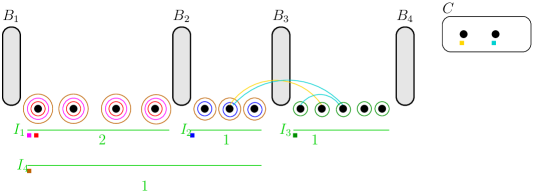
Figure 11: Example of an auxiliary graph. Squares indicate the colors associated to each interval or element of $C.$ For example, $D_{I_{1}}$ is composed of colors pink and red. Notice that there is a rainbow matching.

Definition 12 (Auxiliary graph).

Let $(W,B,C,B^{W_{1}},B^{W_{2}})$ be a partial decomposition and $(\mathcal{I},\textsf{val})$ be its demand. Let also $p=|C|+\sum_{i\in\mathcal{I}_{>0}}\textsf{val}(I).$ We next define the $p$-edge-colored mutigraph $(G,)\langle W,B,C,B^{W_{1}},B^{W_{2}}\rangle$ where the vertex set of $G$ is $W$ and the edges of $G,$ as well as their colors, are defined as follows. We start with $E_{1}=E_{2}=\emptyset.$ Then, for any $c\in C,$ for any $\{u,w\}\subseteq W$ such that $\{u,w,c\}$ is a triangle, we add the edge $e=\{u,w\}$ to $E_{1}$ and we set $(e)=c.$ Moreover, for any $I\in\mathcal{I}_{>0},$ we define a set of new colors $D_{I}$ where $|D_{I}|=\textsf{val}(I).$ Then, for any $u\in D_{I}$ and $v\in W(I),$ we add to $E_{2}$ edge $e=\{v\}$ and we set $(e)=u.$ Finally, we denote $\bigcup_{I\in\mathcal{I}_{>0}}D_{I}$ by $D.$

Notice that if the partial decomposition $(W,B,C,B^{W_{1}},B^{W_{2}})$ is clean, then for any vertex $c\in C$, there exists an edge with color $c$ in $E_{1}$. Notice also that the value of $p$ is a polynomial function of the size $|V(T)|$ of the tournament. In fact, $p=\mathcal{O}(|V(T)|^{3}).$

Definition 13 (Bucket allocation).

Let $(W,B,C,B^{W_{1}},B^{W_{2}})$ be a partial decomposition and $(\mathcal{I},\textsf{val})$ be its demand. A bucket allocation for $(W,B,C,B^{W_{1}},B^{W_{2}})$ is a set $\mathcal{Q}=\{Q_{I},I\in\mathcal{I}_{>0}\}$ such that

• for any $I\in\mathcal{I}_{>0},$ $Q_{I}\subseteq W(I)$

• for any $I\in\mathcal{I}_{>0},$ $|Q_{I}|=\textsf{val}(I)$

• for any $I_{1}$ and $I_{2}$ in $\mathcal{I}_{>0},$ $Q_{I_{1}}\cap Q_{I_{2}}=\emptyset$

We also denote $V(\mathcal{Q})=\bigcup_{I\in\mathcal{I}_{>0}}Q_{I}.$

The next lemma shows that a bucket allocation allows to repack any packing triangle inside ${T}[W\cup B].$

Lemma 17 (Safeness of a bucket allocation for packing).

Let $(W,B,C,B^{W_{1}},B^{W_{2}})$ be a partial decomposition and let $\mathcal{Q}$ be a bucket allocation for $(W,B,C,B^{W_{1}},B^{W_{2}}).$ Let also $\mathcal{P}$ be a triangle-packing with $V(\mathcal{P})\subseteq W\cup B.$ Then, there exists a triangle-packing $\mathcal{P}^{\prime}$ such that

• $V(\mathcal{P}^{\prime})\subseteq V(\mathcal{Q})\cup B$ and

• $|\mathcal{P}^{\prime}|=|\mathcal{P}|$

Proof.

According to Observation 1, we can partition $\mathcal{P}=\mathcal{P}_{1}\cup\mathcal{P}_{2}$ such that, for any $\Delta\in\mathcal{P}_{1},$ $\Delta\subseteq B$ and, moreover, for any $\Delta\in\mathcal{P}_{2},$ there exists $I\in\mathcal{BI}(W,B)$ such that $|\Delta\cap B_{l_{I}}|=|\Delta\cap B_{r_{I}}|=1$ and $\Delta\cap W\subseteq W_{I}.$ Let $A(\mathcal{P}_{2})=\{\Delta\cap B,\Delta\in\mathcal{P}_{2}\}$ be the set of backward arcs used by triangles in $\mathcal{P}_{2}.$

Let us now define an auxiliary graph $H$ that will help us to describe how to repack $\mathcal{P}.$ The vertex set of $H$ is $B$ and for any bucket interval $I=[l_{I},r_{I}]$ of $(W,B),$ we define $E_{I}=\{\{u,v\}\mid u\in B_{l_{I}}\setminus B^{W_{2}}_{l_{I}}\mbox{ or }u\in B_{r_{I}}\setminus B^{W_{2}}_{r_{I}}\},$ and we set $E(H)=\bigcup_{\mathcal{BI}(W,B)}E_{I}.$ Informally, for any $i\neq i^{\prime},$ $H[B_{i}\cup B_{i^{\prime}}]$ is the complete bipartite graph $K_{|B_{i}|,|B^{\prime}_{i}|}$ where we remove all edges between $B^{W_{2}}_{i}$ and $B^{W_{2}}_{i^{\prime}}.$ For any $e\in E(H),$ we denote $I(e)$ the unique bucket interval $I$ such that $e\in E_{I}.$

Observe that $A(\mathcal{P}_{2})\subseteq E(H)$ as for any $\{u,v\}\in A(\mathcal{P}_{2}),$ where $\{u,v\}=\Delta\cap B,$ there exists $I\in\mathcal{BI}(W,B)$ such that $u\in B_{l(I)},$ $v\in B_{r(I)}.$ Moreover, we cannot have $u\in B^{W_{2}}_{l(I)}$ and $v\in B^{W_{2}}_{r(I)},$ as this would imply $\Delta\subseteq W_{0}.$ Finally, as $\mathcal{P}_{2}$ is a packing, $A(\mathcal{P}_{2})$ is even a matching in $H.$

Property $\Pi_{1}.$

Let us prove the following property $\Pi_{1}$:

Property $\Pi_{1}$: For any $I\in\mathcal{BI}(W,B),$ $\textsf{MaxM}(H(I))\leq\mu(I),$ where MaxM denotes the size of a maximum matching, and $H(I)=H[\bigcup_{i\in B(I)}B_{i}].$

Proof of $\Pi_{1}$: Firstly, as any edge in $H(I)$ uses at least one vertex from a set $S_{i}$ for $i\in B(I),$ we deduce that $\textsf{MaxM}(H(I))\leq\Sigma(I).$ Let $i_{0}=\textrm{ argmax}_{i\in B(I)}|B_{i}|.$ Moreover, as for any graph $G^{\prime}$ and any independent set $X^{\prime}\subseteq V(G^{\prime})$ we have $\textsf{MaxM}(G^{\prime})\leq|V(G^{\prime})|-|X^{\prime}|,$ and as $B_{i_{0}}$ is an independent set in $H,$ we get $\textsf{MaxM}(H(I))\leq m(I).$ This implies that $\textsf{MaxM}(H(I))\leq\mu(I).$

Property $\Pi_{2}.$

We proceed by proving property $\Pi_{2}$ which allows us to associate, in a well defined way, a vertex in $V(\mathcal{Q})$ to any arc in $A(\mathcal{P}_{2}).$ An example of this property can be found in Figure 12.

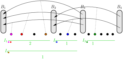
Figure 12: Example of property $\Pi_{2}.$ The bucket allocation is represented by the non-black vertices. Function $f,$ which associates injectively to each backward arc of the initial packing a vertex of the bucket allocation, is depicted using dashed lines.

Property $\Pi_{2}$: For any matching $M$ in $H,$ there is a function $f$ from $M$ to $V(\mathcal{Q})$ such that $f$ is injective and, for any $e\in M,$ $f(e)\in W(I(e))\cap V(\mathcal{Q}).$

Proof of $\Pi_{2}$: Let $U$ be a bipartite graph, where $V(U)=(M,Q),$ and for any $e\in M,$ $N(e)=W(I(e))\cap V(\mathcal{Q}).$ What remains is the proof that there is a perfect matching $f$ (which associates to each $e\in M$ a vertex $f(e)\in N(e)$) in $U$ which saturates $M.$ According to Hall’s Theorem, it is sufficient to prove that, for any $M^{\prime}\subseteq M,$ $|N(M^{\prime})|\geq|M^{\prime}|.$

Let $M^{\prime}\subseteq M.$ Observe that $\bigcup_{e\in M^{\prime}}[l_{I(e)},r_{I(e)}]$ is a union of $t\geq 1$ disjoint intervals denoted $\{I^{\prime}_{1},\dots,I^{\prime}_{t}\},$ and that $M^{\prime}$ can be partitioned into $\bigcup_{i\in[t]}M^{\prime}_{t}$, such that for any $i\in[t],$ $\bigcup_{e\in M^{\prime}_{i}}[l_{I(e)},r_{I(e)}]$ $=I^{\prime}_{i}.$

As an example, consider a matching $M^{\prime}=\{e_{1},e_{2},e_{3},e_{4},e_{5}\}$ where $I(e_{1})=[1,10],I(e_{2})=[3,4],I(e_{3})=[10,11],I(e_{4})=[20,22],I(e_{5})=[21,23],$ $\bigcup_{e\in M^{\prime}}[l_{I(e)},r_{I(e)}]=\{[1,11],[20,23]\}$ and $M^{\prime}_{1}=\{e_{1},e_{2},e_{3}\}.$

Let $i\in[t].$ Observe that, for any $v\in W(I^{\prime}_{i}),$ there exists $e\in M^{\prime}_{i}$ such that $v\in W(I(e)).$ Thus, for any vertex $v\in\bigcup_{I^{\prime}\in P_{\mathcal{I}_{>0}}(I^{\prime}_{i})}Q_{I^{\prime}},$ as $v$ belongs to $W(I^{\prime}_{i}),$ and as there exists $e\in M^{\prime}_{i}$ such that $v\in W(I(e)),$ we get $v\in W(I(e))\cap Q=N(e).$ This implies $\bigcup_{I^{\prime}\in P_{\mathcal{I}_{>0}}(I^{\prime}_{i})}Q_{I^{\prime}}\subseteq N(M^{\prime}_{i}).$ As $Q$ is a bucket allocation for $(W,B,C,B^{W_{1}},B^{W_{2}}),$ we know that the $Q_{I^{\prime}}$ are disjoint and $|Q_{I^{\prime}}|=\textsf{val}(I^{\prime}),$ implying that

$$|\bigcup_{I^{\prime}\in P_{\mathcal{I}_{>0}}(I^{\prime}_{i})}Q_{I^{\prime}}|=\sum_{I^{\prime}\in P_{\mathcal{I}_{>0}}(I^{\prime}_{i})}|Q_{I^{\prime}}|=\sum_{I^{\prime}\in P_{\mathcal{I}_{>0}}(I^{\prime}_{i})}\textsf{val}(I^{\prime})=\textsf{val}(P_{\mathcal{I}_{>0}}(I^{\prime}_{i})).$$

According to Lemma 13, $\textsf{val}(P_{\mathcal{I}_{>0}}(I^{\prime}_{i}))\geq\mu(I^{\prime}_{i}).$ According to Property $\Pi_{1},$ $\mu(I^{\prime}_{i})\geq\textsf{MaxM}(H(I^{\prime}_{i})).$ This implies that $|N(M^{\prime}_{i})|\geq\textsf{MaxM}(H(I^{\prime}_{i})).$ Since $M^{\prime}$ is a matching in $H,$ $M^{\prime}_{i}$ is a matching in $H(I^{\prime}_{i}).$ This implies $\textsf{MaxM}(H(I^{\prime}_{i}))\geq|M^{\prime}_{i}|$ and therefore $|N(M^{\prime}_{i})|\geq|M^{\prime}_{i}|.$ To conclude, let us now consider the partition $\{N(M^{\prime}_{i})\mid i\in[t]\}$ of $N(M^{\prime}).$ As the $N(M^{\prime}_{i})$s are vertex-disjoint, we get

$$|N(M^{\prime})|=\sum_{i\in[t]}|N(M^{\prime}_{i})|\geq\sum_{i\in[t]}\textsf{MaxM}(H(I^{\prime}_{i})).$$

As $M^{\prime}$ is a matching in $\bigcup_{i\in[t]}H(I^{\prime}_{i}),$ and as $\sum_{i\in[t]}\textsf{MaxM}(H(I^{\prime}_{i}))\geq\textsf{MaxM}(\bigcup_{i\in[t]}H(I^{\prime}_{i})),$ we conclude that $|N(M^{\prime})|\geq|M^{\prime}|.$

We can now conclude the proof of Lemma. As $A(\mathcal{P}_{2})$ is a matching in $H,$ by Property $\Pi_{2},$ there is a function $f$ from $A(\mathcal{P}_{2})$ to $V(\mathcal{Q})$ such that $f$ is injective and, for any $e\in A(\mathcal{P}_{2}),$ $f(e)\in W(I(e))\cap V(\mathcal{Q}).$ By Observation 1, $e\cup f(e)$ is still a triangle. Thus, we define $\mathcal{P}^{\prime}_{2}=\{e\cup f(e),e\in A(\mathcal{P}_{2})\}$ and $\mathcal{P}^{\prime}=\mathcal{P}_{1}\cup\mathcal{P}^{\prime}_{2}.$ As $V(\mathcal{P}^{\prime}_{2})\cap B=V(\mathcal{P}_{2})\cap B$ and as $f$ is injective, $\mathcal{P}^{\prime}$ is still a triangle-packing, and $|\mathcal{P}^{\prime}|=|\mathcal{P}|.$ Moreover, as $V(\mathcal{P}_{1})\subseteq B$ and $V(\mathcal{P}^{\prime}_{2})\subseteq B\cup V(\mathcal{Q}),$ we get $V(\mathcal{P}^{\prime})\subseteq B\cup V(\mathcal{Q}).$ ∎

Finally, the last lemma of the section indicates how to build a feedback vertex set of $T[W\cup B]$ with the help of a bucket allocation. This will be usefull for the kernel of FVST designed Section 5. We enounce this lemma here, as the notations and the techniques used in its proof are similar, though easier, than in the previous lemma.

Lemma 18 (Safeness of a bucket allocation for hitting).

Let $(W,B,C,B^{W_{1}},B^{W_{2}})$ be a partial decomposition and let $\mathcal{Q}$ be a bucket allocation for $(W,B,C,B^{W_{1}},B^{W_{2}}).$ Let also $X$ be a feedback vertex set of $T[V(\mathcal{Q})\cup B]$. Then, there exists $X^{\prime}$ a feedback vertex set of $T[W\cup B]$ with $|X^{\prime}|\leq|X|$.

Proof.

We partition $X$ into two sets $X_{B}=X\cap B$ and $X_{\mathcal{Q}}=X\cap V(\mathcal{Q})$. And we define $H$ being the graph on vertex set $B$ and with edge set $\{uv\ :\ uv\in A(T),u\in B_{i}\setminus X_{B},v\in B_{j}\setminus X_{B}\textrm{ with }j<i\}$. Informally, from $T[B]$ we only keep in $H$ the backward arcs between the $B_{i}$’s not incident with vertices of $X_{B}$. Notice that in particular, there is no edge in $H$ between any two $B_{i}^{W_{2}}$, as there where originally part of $W_{0}$.

Property $\Pi_{1}^{\prime}.$

Let us prove the following property $\Pi_{1}^{\prime}$:

Property $\Pi_{1}^{\prime}$: For any $I\in\mathcal{BI}(W,B),$ $\textsf{MinVC}(H(I))\leq\mu(I),$ where MinVC denotes the size of a minimum vertex cover, and $H(I)=H[\bigcup_{i\in B(I)}B_{i}].$

Proof of $\Pi_{1}^{\prime}$: As every edge of $H$ is incident with a vertex of one $S_{i}$ (which is $B_{i}\setminus B_{i}^{W_{2}}$), the set $\cup_{i}S_{i}$ is a vertex cover of $H$, and then $\textsf{MinVC}(H(I))\leq\Sigma(I)$. Similarly, let $i_{0}=\textrm{ argmax}_{i\in B(I)}|B_{i}|$, the set $(\cup_{i}B_{i})\setminus B_{i_{0}}$ is clearly a vertex cover of $H$. Then we get $\textsf{MinVC}(H(I))\leq m(I)$, and finally conclude that $\textsf{MinVC}(H(I))\leq\mu(I)$.

Now, let us consider an arc $uv$ of $T$ such that $uv\in E(H)$. We have $u\in B_{i}$ and $v\in B_{j}$ for some $j<i$ and denote by $I$ the bucket interval $[j,i]$. By Observation 1, $uvw$ is a triangle for every vertex $w$ of $W(I)$. In particular, for every $w\in W(I)\cap V(\mathcal{Q})$ we must have $w\in X_{\mathcal{Q}}$.
So, denote by $\cal J$ the set of bucket intervals whose extremities contains the end of an edge of $H$ (formally, $[j,i]\in{\cal J}$ if there exists $uv\in E(H)$ with $u\in B_{i}$ and $v\in B_{j}$). Let $J^{\star}$ be a block of the block partition of $\cal J$, meaning that $J^{\star}$ is a non-empty, inclusion-wise minimal bucket interval with the property that for every $J\in{\cal J}$, either $J\cap J^{\star}=\emptyset$ or $J\subseteq J^{\star}$. By the previous remark remark, we know that $X_{\mathcal{Q}}$ contains at least $|W(J^{\star})\cap V(\mathcal{Q})|$ vertices in $W(J^{\star})$. As $\mathcal{Q}$ is a bucket allocation, we have in particular that $|W(J^{\star})\cap V(\mathcal{Q})|=|\cup\{Q_{J}\ :\ Q_{J}\in{\cal Q}\textrm{ and }J\subseteq J^{\star}\}|=\textsf{val}(P_{\mathcal{I}}(J^{\star}))\geq\mu(J^{\star})$ by Lemma 13.

Finally, by Property $Pi_{1}^{\prime}$, there exists a vertex cover $X_{J^{\star}}^{\prime}$ of $H(J^{\star})$ containing at most $\mu(J^{\star})\leq|W(J^{\star})\cap X_{\mathcal{Q}}|$ vertices. Considering all the block intervals $J_{1}^{\star},\dots,J_{p}^{\star}$ of $\cal J$, we obtain a vertex cover $X^{\prime}_{\mathcal{Q}}=\cup_{j}X_{J_{j}^{\star}}^{\prime}$ of $H$ such that $|X^{\prime}_{\mathcal{Q}}|\leq|X_{\mathcal{Q}}|$. In particular, for every arc $uv$ of $T$ with $u\in B_{i}$ and $v\in B_{j}$ with $j<i$ we have $u\in X^{\prime}_{\mathcal{Q}}\cup X_{B}$ or $u\in X^{\prime}_{\mathcal{Q}}\cup X_{B}$.
We now define $X^{\prime}=X^{\prime}_{\mathcal{Q}}\cup X_{B}$. We have $|X^{\prime}|\leq|X|$ and $X^{\prime}$ is a feedback vertex set of $T[W\cup B]$. Indeed, let $\Delta$ by a triangle of $T[W\cup B]$. If $V(\Delta)\subseteq B$, then $V(\Delta)\cap X_{B}\neq\emptyset$. Otherwise, as $(W,B)$ is a nice pair, there exist buckets $B_{i}$ and $B_{j}$ with $j<i$ such that $\Delta=uvw$ with $u\in B_{i}$, $v\in B_{j}$ and $w\in W_{[j,i]}$. But in this case we must have $u\in X^{\prime}_{\mathcal{Q}}$ or $v\in X^{\prime}_{\mathcal{Q}}$. ∎

6.7 Operations on buckets

Our kernelization algorithm has only one rule that is applied exhaustively. Each application of the this rule (except the last one that finds a rainbow matching) triggers an “add” operation, defined below, where we add new vertices to the buckets. In this section, we define the two variants of the add operation and prove that, given a partial decomposition, these operations output another partial decomposition.

Definition 14.

Let $(W,B,C,B^{W_{1}},B^{W_{2}})$ be a partial decomposition. Let $U\subseteq W$ and $X^{C}\subseteq C.$ For any $j\in\{1,2\},$ we define $\textsf{add}_{j}(W,B,B^{W_{1}},B^{W_{2}},U\cup X^{C})$ as $(W^{\prime},B^{\prime},C^{\prime},B^{{}^{\prime}W_{1}},B^{{}^{\prime}W_{2}})$ where

• $W^{\prime}=W\setminus U$

• $B^{\prime}=B\cup U\cup X^{C}$

• $C^{\prime}=C\setminus X^{C}$

• $B^{{}^{\prime}W_{j}}=B^{W_{j}}\cup U$ and $B^{{}^{\prime}W_{3-j}}=B^{W_{3-j}}.$

Figure 13: An application of $\textsf{add}_{1}$ (or $\textsf{add}_{2}$). Vertices of $U$ are inside the green territories and the two vertices of $X^{C}$ are the two non-filled vertices. We have $S^{\psi}=\{8,14,20,\infty\}$ and $S^{\psi^{\prime}}=\{8,13,22,\infty\}.$

Lemma 19.

Let $(W,B,C,B^{W_{1}},B^{W_{2}})$ be a partial decomposition of local size $f.$ Suppose $f(x)=cx^{\delta}$ for some constants $c$ and $\delta,$ where $\delta>1.$ Let $U\subseteq W$ and $X^{C}\subseteq C$ such that $|U|\leq 10|X^{C}|$ and such that, for any triangle $\Delta$ of ${T}[W\cup X^{C}],$ we have that $|\Delta\cap(W\setminus U)|\leq 1.$ Then, $\textsf{add}_{1}(W,B,B^{W_{1}},B^{W_{2}},U\cup X^{C})$ is a partial decomposition of local size $f.$

Proof.

Let $(W^{\prime},B^{\prime},C^{\prime},B^{{}^{\prime}W_{1}},B^{{}^{\prime}W_{2}})=\textsf{add}_{1}(W,B,B^{W_{1}},B^{W_{2}},U\cup X^{C}).$ We begin by proving that $(W^{\prime},B^{\prime},C^{\prime},B^{{}^{\prime}W_{1}},B^{{}^{\prime}W_{2}})$ is a partial decomposition. Properties 1 and 2 are clear. As, by assumption, for any triangle $\Delta$ of ${T}[W\cup X^{C}],$ we have that $|\Delta\cap(W\setminus U)|\leq 1,$ Lemma 10 implies that $\psi^{\prime}=(W^{\prime},B^{\prime})$ is a nice pair, and thus we obtain Property 3.

Let us now prove Property 4. We start by proving the following structural property of the $B^{\prime}_{i}$ (see Figure 13).

For any $i\in S^{\psi^{\prime}},$ $\exists U^{\prime}\subseteq U,$ $X^{\prime}\subseteq X^{C}$ and $S^{\prime}\subseteq S^{\psi}$ such that $B^{\prime}_{i}=\bigcup_{i\in S^{\prime}}B_{i}\cup X^{\prime}\cup U^{\prime}.$

We point out that we could even prove a stronger property (for example that buckets in $S^{\prime}$ are consecutive), but we don’t need it in the remainder of the proof.

Let $i\in\psi^{\prime}.$ According to Proposition 1, $B^{\prime}_{i}$ is the set of vertices $v$ of $B^{\prime}$ such that all arcs between $W^{\prime}_{[1,i-1]}$ and $v$ are oriented from $W^{\prime}_{[1,i-1]}$ to $v$ and all arcs between $W^{\prime}_{[i,t_{0}]}$ and $v$ are oriented from $v$ to $W^{\prime}_{[i,t_{0}]}.$ Assume that there exists $j\in\psi$ and $v_{1}\in B_{j}$ such that $v_{1}\in B^{\prime}_{i}.$ Now, observe that for any $v_{2}\in B_{j}$ and $w\in W^{\prime},$ $v_{1}w\in A({T})$ iff $v_{2}w\in A({T}),$ and the same holds for $wv_{1}$ and $wv_{2}.$ This implies that $v_{2}\in B^{\prime}_{i}$ and thus $B_{j}\subseteq B^{\prime}_{i}.$ As all the vertices we add to $B$ are from $U\cup X^{C},$ this proves the above structural property.

Next we prove that $(B^{{}^{\prime}W_{1}},B^{{}^{\prime}W_{2}})$ is a bucket partition of $(W^{\prime},B^{\prime}).$ The fact that $(B^{{}^{\prime}W_{1}},B^{{}^{\prime}W_{2}})$ is a partition of $B^{{}^{\prime}W}$ is clear, as $B^{{}^{\prime}W}=B^{W}\cup U,$ $B^{{}^{\prime}W_{1}}=B^{W_{1}}\cup U,$ and $B^{{}^{\prime}W_{2}}=B^{W_{2}}.$ Let $i\in S^{\psi^{\prime}}.$ By the previous structural property, $B^{\prime}_{i}=\bigcup_{i\in S^{\prime}}B_{i}\cup X^{\prime}\cup U^{\prime}.$ If $S^{\prime}\neq\emptyset,$ then $|S^{\prime}_{i}|\geq\bigcup_{i\in S^{\prime}}|S_{i}|\geq 1.$ Otherwise, as $X^{\prime}\cup U^{\prime}\neq\emptyset,$ $U^{\prime}\subseteq B^{{}^{\prime}W_{1}}$ and $X^{\prime}\subseteq B^{{}^{\prime}C}_{i},$ we get $U^{\prime}\cup X^{\prime}\subseteq S^{{}^{\prime}}_{i},$ implying $|S^{\prime}_{i}|\geq 1.$ Let us prove that $|B^{{}^{\prime}W_{1}}|\leq 10|B^{{}^{\prime}C}|.$

$$|B^{{}^{\prime}W_{1}}| = |B^{W_{1}}|+|U|$$

$$\leq 10|B^{C}|+|U|$$

$$\leq 10|B^{C}|+10|X^{C}|$$

$$= 10|B^{{}^{\prime}C}|.$$

This concludes the proof that $(B^{{}^{\prime}W_{1}},B^{{}^{\prime}W_{2}})$ is a bucket partition of $(W^{\prime},B^{\prime}).$

Let us finally prove that $(B^{{}^{\prime}W_{1}},B^{{}^{\prime}W_{2}})$ has local size $f,$ meaning that for any $i\in S^{\psi^{\prime}},$ we have $|B_{i}^{{}^{\prime}W_{2}}|\leq f(|S^{\prime}_{i}|)=c|S_{i}^{\prime}|^{\delta}.$ Let $i\in S^{\psi^{\prime}}.$ By the previous structural property, there exists $S^{\prime}\subseteq S^{\psi}$ such that $S^{\prime}_{i}\supseteq\bigcup_{j\in S^{\prime}}S_{j}.$ In particular, we have $|S^{\prime}_{i}|\geq\sum_{j\in S^{\prime}}|S_{j}|$ as the $S_{j}$’s are disjoint. Now, noticing that $B^{\prime W_{2}}=B^{W_{2}},$ we have the following.

$$|B_{i}^{{}^{\prime}W_{2}}| = |\bigcup_{i\in S^{\prime}}B_{i}\cap B^{{}^{\prime}W_{2}}|+|(X^{\prime}\cup U^{\prime})\cap B^{{}^{\prime}W_{2}}|$$

$$= |\bigcup_{i\in S^{\prime}}B_{i}\cap B^{W_{2}}|+0$$

$$\leq \sum_{i\in S^{\prime}}c|S_{i}|^{\delta}$$

$$\leq c(\sum_{i\in S^{\prime}}|S_{i}|)^{\delta}$$

$$\leq c|S^{\prime}_{i}|^{\delta}.$$

∎

Now, we analyze the $\textsf{add}_{2}$ operation.

Lemma 20.

Let $(W,B,C,B^{W_{1}},B^{W_{2}})$ be a partial decomposition of local size $f.$ Suppose $f(x)=cx^{\delta}$ for some constants $c$ and $\delta,$ where $1<\delta\leq 2$ and $c\geq\max(\frac{20}{(2^{\delta}-2)},(\frac{21}{\delta})^{\frac{1}{\delta-1}}).$ Let $I$ be a bucket interval and $U=W(I)$ such that $|U|\leq 10\mu(I).$ Then, $\textsf{add}_{2}(W,B,B^{W_{1}},B^{W_{2}},U)$ is a partial decomposition of local size $f.$

Proof.

Let $(W^{\prime},B^{\prime},C^{\prime},B^{{}^{\prime}W_{1}},B^{{}^{\prime}W_{2}})=\textsf{add}_{2}(W,B,B^{W_{1}},B^{W_{2}},U).$ As a first step we prove that $(W^{\prime},B^{\prime},C^{\prime},B^{{}^{\prime}W_{1}},B^{{}^{\prime}W_{2}})$ is a partial decomposition. Properties 1 and 2 are clear. By applying Lemma 10 (for $X^{C}=\emptyset$ here), we get that $\psi^{\prime}=(W^{\prime},B^{\prime})$ is a nice pair, and thus we obtain Property 3.

Let us now prove Property 4. Let us first describe the bucket decomposition in $\psi^{\prime}.$ Informally, all buckets of $B(I)$ are merged, together with $U,$ into a new one ($B^{\prime}_{r_{I}}$), and all the other buckets remain unchanged. More formally, the following three properties hold

• $S^{\psi^{\prime}}=(S^{\psi}\setminus B(I))\cup\{r_{I}\},$

• for any $i\in S^{\psi^{\prime}}\setminus\{r_{I}\},$ it holds that

  • $B^{\prime}_{i}=B_{i},$

  • $B^{C}_{i}=B_{i},$ and

  • for any $j\in[2],$ $B^{{}^{\prime}W_{j}}_{i}=B^{W_{j}}_{i},$

• $B^{\prime}_{r_{I}}=U\cup\bigcup_{i\in B(I)}B_{i}.$

The next step is to prove that $(B^{{}^{\prime}W_{1}},B^{{}^{\prime}W_{2}})$ is a bucket partition of $(W^{\prime},B^{\prime}).$ The fact that $(B^{{}^{\prime}W_{1}},B^{{}^{\prime}W_{2}})$ is a partition of $B^{{}^{\prime}W}$ is clear as $B^{{}^{\prime}W}=B^{W}\cup U,$ $B^{{}^{\prime}W_{1}}=B^{W_{1}}$ and $B^{{}^{\prime}W_{2}}=B^{W_{2}}\cup U.$ Let $i\in S^{\psi^{\prime}}.$ If $i\in S^{\psi^{\prime}}\setminus\{r_{I}\},$ then, by the previous property, we get $S^{\prime}_{i}=S_{i},$ implying $|S^{\prime}_{i}|\geq 1,$ as $(B^{W_{1}},B^{W_{2}})$ is a bucket partition of $(W,B).$ If $i=r_{I},$ then $B^{\prime}_{r_{I}}\supseteq\bigcup_{i\in B(I)}B_{i}$ and, as $B^{{}^{\prime}W_{1}}=B^{W_{1}},$ $|S^{\prime}_{r_{I}}|\geq\sum_{i\in B(I)}|S^{\prime}_{i}|\geq|B(I)|\geq 2.$ Moreover, we have $|B^{{}^{\prime}W_{1}}|=|B^{W_{1}}|\leq 10|B^{C}|=10|B^{{}^{\prime}C}|.$ This concludes the proof that $(B^{{}^{\prime}W_{1}},B^{{}^{\prime}W_{2}})$ is a bucket partition of $(W^{\prime},B^{\prime}).$

Let us finally prove that $(B^{{}^{\prime}W_{1}},B^{{}^{\prime}W_{2}})$ has local size $f,$ meaning that, for any $i\in S^{\psi^{\prime}},$ $|B_{i}^{{}^{\prime}W_{2}}|\leq f(|S^{\prime}_{i}|).$ Recall that $(W^{\prime},B^{\prime})$ is a nice pair, implying, because of Proposition 1, that there is a unique bucket decomposition $B^{\prime}_{i}$ of $B^{\prime}.$ Thus, for any $i\in S^{\psi^{\prime}}\setminus\{r_{I}\},$ $|B^{{}^{\prime}W_{2}}_{i}|=|B^{W_{2}}_{i}|\leq f(|S_{i}|)=f(|S^{\prime}_{i}|).$

Let $B(I)=\{i_{1},\dots,i_{L}\}$, where $|S_{i_{x}}|\geq|S_{i_{x+1}}|,$ for any $x$. Notice that $f(|S^{\prime}_{r_{I}}|)=c|S^{\prime}_{r_{I}}|^{\delta}=c(\sum_{\ell\in[1,L]}S_{i_{\ell}})^{\delta}$, and that $m(I)=\sum_{i\in B(I)}|B_{i}|-|B_{i_{*}}|$ where $i_{*}=\textrm{ argmax}_{i\in B(I)}|B(i)|$, implying that $m(I)\leq\sum_{\ell\in[2,L]}|B_{i_{\ell}}|\leq\sum_{\ell\in[2,L]}(|B_{i_{\ell}}^{W_{2}}|+|S_{i_{\ell}}|)\leq\sum_{\ell\in[2,L]}(c|S_{i_{\ell}}|^{\delta}+|S_{i_{\ell}}|)$. It remains to prove that $|B^{{}^{\prime}W_{2}}_{r_{I}}|-f(|S^{\prime}_{r_{I}}|)\leq 0$.

Observe that

$$|B^{{}^{\prime}W_{2}}_{r_{I}}|-f(|S^{\prime}_{r_{I}}|) = \sum_{i\in B(I)}|B^{W_{2}}_{i}|+|U|-c(\sum_{\ell\in[1,L]}|S_{i_{\ell}}|)^{\delta}$$

$$\leq \sum_{i\in B(I)}|B^{W_{2}}_{i}|+10\min\big{\{}\Sigma(I),m(I)\big{\}}-c(\sum_{\ell\in[1,L]}|S_{i_{\ell}}|)^{\delta}$$

$$\leq c|S_{i_{1}}|^{\delta}+c\sum_{\ell\in[2,L]}|S_{i_{\ell}}|^{\delta}+$$

$$\phantom{c|S_{i_{1}}|^{\delta}+}\leavevmode\nobreak\ 10\min\big{\{}\sum_{i\in B(I)}|S_{i}|,\sum_{\ell\in[2,L]}(c|S_{i_{\ell}}|^{\delta}+|S_{i_{\ell}}|)\big{\}}-c(\sum_{\ell\in[1,L]}|S_{i_{\ell}}|)^{\delta}$$

$$= \min\big{\{}f_{1}(S_{i_{1}}),f_{2}(S_{i_{1}})\big{\}},$$

where

• $f_{1}(x)=cx^{\delta}+c\sum_{\ell\in[2,L]}|S_{i_{\ell}}|^{\delta}+10(x+\sum_{\ell\in[2,L]}|S_{i_{\ell}}|)-c(x+\sum_{\ell\in[2,L]}|S_{i_{\ell}}|)^{\delta}$

• $f_{2}(x)=cx^{\delta}+c\sum_{\ell\in[2,L]}|S_{i_{\ell}}|^{\delta}+10\sum_{\ell\in[2,L]}(c|S_{i_{\ell}}|^{\delta}+|S_{i_{\ell}}|)-c(x+\sum_{\ell\in[2,L]}|S_{i_{\ell}}|)^{\delta}$

Let $g:\mathbb{R}^{+}\to\mathbb{R}^{+}$ be such that $g(x)=(x+\sum_{\ell\in[2,L]}S_{i_{\ell}})^{\delta}-x^{\delta}$ and observe that it is a non-decreasing function, as $\delta>1$. Therefore

$$f_{2}(x)=c\sum_{\ell\in[2,L]}|S_{i_{\ell}}|^{\delta}+10\sum_{\ell\in[2,L]}(c|S_{i_{\ell}}|^{\delta}+|S_{i_{\ell}}|)-cg(x),$$

and thus $f_{2}$ a non-increasing function. Let $x_{0}=\sum_{\ell\in[2,L]}|S_{i_{\ell}}|^{\delta}$. Notice that according to the first property of a bucket partition, for any $i\in S^{\psi},$ we have $|S_{i}|\geq 1$, implying that $x_{0}\geq L-1\geq 1$.

To complete the proof we distinguish two cases according to the value of $|S_{i_{1}}|$. However, before we proceed with these two cases, we prove a helpful claim.

Claim 1:

Let $g_{2}(x)=c^{\delta}x^{\delta}+21x-(cx+x^{\frac{1}{\delta}})^{\delta}$. For $x\geq 0$, $\delta>1$ and $c\geq(\frac{21}{\delta})^{\frac{1}{\delta-1}}$, we have $g_{2}(x)\leq 0$.

Proof of Claim 1: We have

$$(cx+x^{\frac{1}{\delta}})^{\delta} = c^{\delta}x^{\delta}(1+\frac{x^{\frac{1}{\delta}-1}}{c})^{\delta}$$

$$\geq c^{\delta}x^{\delta}(1+\delta\frac{x^{\frac{1}{\delta}-1}}{c})\mbox{ as $(1+u)^{\alpha}\geq 1+\alpha u$ for any $\alpha>1$ and $u>0$}$$

$$= c^{\delta}x^{\delta}+\delta c^{\delta-1}x^{\frac{1}{\delta}-1+\delta}$$

Thus,

$$g_{2}(x) \leq 21x-\delta c^{\delta-1}x^{\frac{1}{\delta}-1+\delta}$$

$$\leq 21x-\delta c^{\delta-1}x\mbox{ as $\frac{1}{\delta}-1+\delta=\frac{\delta^{2}-2\delta+1}{\delta}+1=\frac{(\delta-1)^{2}}{\delta}+1\geq 1$ }$$

$$\leq 0\mbox{\leavevmode\nobreak\ \leavevmode\nobreak\ \leavevmode\nobreak\ as $c\geq(\frac{21}{\delta})^{\frac{1}{\delta-1}}$}$$

This implies that $g_{2}(x)\leq 0$ for any $x\geq 0$. This completes the proof of Claim 1.

Now that Claim 1 is proved, let us come back to our two cases.

Case 1 : if $|S_{i_{1}}|\geq cx_{0}$.

In this case, we will prove that $f_{2}(|S_{i_{1}}|){\leq}0$. As $f_{2}$ is non-increasing, we get $f_{2}(|S_{i_{1}}|)\leq f_{2}(cx_{0})$ therefore, it remains to prove that $f_{2}(cx_{0})\leq 0$. Observe that as $\delta\geq 1$, $(\sum_{\ell\in[2,L]}|S_{i_{\ell}}|)^{\delta}\geq\sum_{\ell\in[2,L]}|S_{i_{\ell}}|^{\delta}$, implying that $(\sum_{\ell\in[2,L]}|S_{i_{\ell}}|)\geq x_{0}^{\frac{1}{\delta}}$. Observe that

$$f_{2}(cx_{0}) \leq cc^{\delta}x_{0}^{\delta}+cx_{0}+20cx_{0}-c(cx_{0}+x_{0}^{\frac{1}{\delta}})^{\delta}\iff$$

$$\frac{f_{2}(cx_{0})}{c} \leq c^{\delta}x_{0}^{\delta}+21x_{0}-(cx_{0}+x_{0}^{\frac{1}{\delta}})^{\delta}=g_{2}(x_{0})$$

The assertion in this case now follows from Claim 1.

Case 2 : if $|S_{i_{1}}|<cx_{0}$.

In this case, we will prove that $f_{1}(|S_{i_{1}}|)\geq 0$. Let us first prove that $f_{1}$ is convex.

$$\frac{d^{2}}{dx^{2}}f_{1}(x) = c(\delta)(\delta-1)(x^{\delta-2}-(x+\sum_{\ell\in[2,L]}S_{i_{\ell}})^{\delta-2})$$

$$\geq 0,\mbox{ as $\delta\leq 2$}$$

Thus, as $|S_{i_{2}}|\leq|S_{i_{1}}|<cx_{0}$, by the definition of the $S_{i_{j}}$, and $f_{1}$ is convex, $f_{1}(|S_{i_{1}}|)\leq\max(f_{1}(|S_{i_{2}}|),f_{1}(cx_{0}))$. Let us prove that both these values are lower or equal to zero. Observe that $\frac{f_{1}(cx_{0})}{c}\leq g_{2}(x_{0})\leq 0$ by Claim 1, and thus it remains to prove that $f_{1}(|S_{i_{2}}|)\leq 0$.

For any $x_{i}\geq 0$, let $f(x_{2},\dots,x_{L})=2c^{\delta}x_{2}^{\delta}+c\sum_{\ell\in[3,L]}x_{\ell}^{\delta}+10(2x_{2}+\sum_{\ell\in[3,L]}x_{\ell})-c(2x_{2}+\sum_{\ell\in[3,L]}x_{\ell})^{\delta}$. Observe that $f_{1}(|S_{i_{2}}|)=f(|S_{i_{2}}|,|S_{i_{3}}|,\dots,|S_{i_{L}}|)$.

Claim 2:

For any tuple of integers $(x_{2},\dots,x_{L})$ where $x_{\ell}\geq 1$ for any $\ell\in[2,L]$, $f(x_{2},\dots,x_{L})\leq f(x_{2},0,\dots,0)$.

Proof of Claim 2: Let $(x_{2},\dots,x_{L})$ be a tuple of integers where $x_{\ell}\geq 0$. Let $i_{0}\in[3,L]$ such that $x_{i_{0}}\geq 1$, and $x^{\prime}_{i_{0}}=x_{i_{0}}-1$. Let $D=f(x_{2},\dots,x_{i_{0}},\dots,x_{L})-f(x_{2},\dots,x^{\prime}_{i_{0}},\dots,x_{L})$. Our goal is to prove that $D\leq 0$. Repeating the decrementation, this will imply Claim $2$.

$$D = cx_{i_{0}}^{\delta}-c(x_{i_{0}}-1)^{\delta}+10-c(\alpha^{\delta}-(\alpha-1)^{\delta})\mbox{ \leavevmode\nobreak\ \leavevmode\nobreak\ \leavevmode\nobreak\ \leavevmode\nobreak\ \leavevmode\nobreak\ ( where $\alpha=2x_{2}+\sum_{\ell\in[3,L]}x_{\ell}$)}$$

$$\leq c(x_{i_{0}}^{\delta}-(x_{i_{0}}-1)^{\delta}-(3x_{i_{0}})^{\delta}+(3x_{i_{0}}-1)^{\delta})+10\mbox{ \leavevmode\nobreak\ \leavevmode\nobreak\ \leavevmode\nobreak\ \leavevmode\nobreak\ \leavevmode\nobreak\ (as $D$ is non increasing in $\alpha$, and $\alpha\geq 3x_{i_{0}}$)}$$

For any $y\geq 1$, let $u(y)=y^{\delta}-(y-1)^{\delta}-(3y)^{\delta}+(3y-1)^{\delta}$. Let us first lower bound two different parts of $u$. We have

$$(y-1)^{\delta} = y^{\delta}(1-\frac{1}{y})^{\delta}$$

$$\geq y^{\delta}(1-\frac{\delta}{y})\mbox{ \leavevmode\nobreak\ \leavevmode\nobreak\ \leavevmode\nobreak\ \leavevmode\nobreak\ \leavevmode\nobreak\ (as $(1-u)^{\alpha}\geq 1-\alpha u$ for any $\alpha>1$ and $0\leq u\leq 1$)}$$

$$= y^{\delta}-\delta y^{\delta-1}$$

Moreover, denoting $z=3y-1$, we have

$$(3y)^{\delta} = (z+1)^{\delta}$$

$$= z^{\delta}(1+\frac{1}{z})^{\delta}$$

$$\geq z^{\delta}(1+\frac{\delta}{z})\mbox{ \leavevmode\nobreak\ \leavevmode\nobreak\ \leavevmode\nobreak\ \leavevmode\nobreak\ \leavevmode\nobreak\ (as $(1+u)^{\alpha}\geq 1+\alpha u$ for any $\alpha>1$ and $u>0$)}$$

$$= z^{\delta}+\delta z^{\delta-1}$$

$$= (3y-1)^{\delta}+\delta(3y-1)^{\delta-1}$$

Using these two lower bounds, we get

$$u(y) \leq \delta(y^{\delta-1}-(3y-1)^{\delta-1})$$

$$\leq \delta(1-2^{\delta-1})\mbox{ \leavevmode\nobreak\ \leavevmode\nobreak\ \leavevmode\nobreak\ \leavevmode\nobreak\ \leavevmode\nobreak\ (as $y^{\delta-1}-(3y-1)^{\delta-1}$ is decreasing in $y$ and $y\geq 1$)}$$

This implies

$$D \leq cu(x_{i_{0}})+10$$

$$\leq c\delta(1-2^{\delta-1})+10$$

$$\leq 0\mbox{ \leavevmode\nobreak\ \leavevmode\nobreak\ \leavevmode\nobreak\ \leavevmode\nobreak\ \leavevmode\nobreak\ (as $c\geq\frac{20}{(2^{\delta}-2)}\geq\frac{10}{\delta(2^{\delta-1}-1)}$ for $\delta\geq 1$)}$$

Concluding the proof of Claim 2.

Let us now come back to the end of proof of Case 2. We had:

$$f_{1}(|S_{i_{2}}|) = f(|S_{i_{2}}|,|S_{i_{3}}|,\dots,|S_{i_{L}}|)$$

$$\leq f(|S_{i_{2}}|,0,\dots,0)\mbox{ by Claim $2$}$$

$$= 2c^{\delta}|S_{i_{2}}|^{\delta}+20|S_{i_{2}}|-c(2|S_{i_{2}}|)^{\delta}$$

$$= c|S_{i_{2}}|^{\delta}(2-2^{\delta})+20|S_{i_{2}}|\mbox{ \leavevmode\nobreak\ \leavevmode\nobreak\ \leavevmode\nobreak\ \leavevmode\nobreak\ \leavevmode\nobreak\ ( which is decreasing in $|S_{i_{2}}|$ as $c\geq\frac{20}{(2^{\delta}-2)}$ and $\delta\geq 1$)}$$

$$\leq c(2-2^{\delta})+20\mbox{ \leavevmode\nobreak\ \leavevmode\nobreak\ \leavevmode\nobreak\ \leavevmode\nobreak\ \leavevmode\nobreak\ (as $|S_{i_{2}}|\geq 1$)}$$

$$\leq 0\mbox{ \leavevmode\nobreak\ \leavevmode\nobreak\ \leavevmode\nobreak\ \leavevmode\nobreak\ \leavevmode\nobreak\ (as $c\geq\frac{20}{(2^{\delta}-2)}$ and $\delta\geq 1$)}$$

This concludes the proof of Case 2. ∎

Discussion on why a simpler definition of $\mu$ is not sufficient.

We explain here why taking simply $\mu(I)=\text{\tt{\Sigma}}(I)$ or $\mu(I)=m(I)$ (instead of $\mu(I)=\min(\text{\tt{\Sigma}}(I),m(I))$) would not be sufficient to get a kernel in $\mathcal{O}(k^{\delta})$ for any $\delta>1$. Let us assume that the current partial decomposition is $(W,B,C,B^{W_{1}},B^{W_{2}})$ where in particular $S^{\psi}=\{i_{1},\dots,i_{k^{\prime}}\}$ for $k^{\prime}=\frac{k}{2}$, $B^{W_{j}}=\emptyset$ for $j\in\{1,2\}$, implying that buckets only contain vertices of $C^{0}$, and $|B_{i}|=1$ for any $i\in S^{\psi}$. Suppose that $k=2^{x}$ for some $x$.

Suppose first that we define $\mu(I)=\text{\tt{\Sigma}}(I)$. Notice that particular $\textsf{val}([i_{1},i_{2}])=\mu([i_{1},i_{2}])=2$, and thus that in the auxiliary graph we will have in particular two colors $d_{1}$, $d_{2}$ such that all vertices of $W([i_{1},i_{2}])$ have one loop of color $d_{1}$ and one loop of color $d_{2}$. The kernel now applies its unique reduction rule (see Definition 15). Suppose that we do not find a rainbow matching, and that the set of color we find using Corollary 1 is $X=\{d_{1},d_{2}\}$, and thus that the small associated vertex cover is the set $U=W([i_{1},i_{2}])$ ($U$ must cover all these loops), where $|U|=5|X|=10$. In this case, we fall into Case 2, and the $add_{2}$ operation will merge $B_{i_{1}}$, $B_{i_{2}}$ and $W([i_{1},i_{2}])$ into a new bucket $B^{\prime}_{i_{2}}$. If we now repeat the same scenario between $B^{\prime}_{i_{2}}$ and $B_{i_{3}}$, we will now have $\mu(I)=3$ (where $I=[i_{2},i_{3}]$), and thus $|U|\leq 15$. Thus, if we repeat again until all buckets are merged into a single one, the total number of vertices of $W$ added to buckets during these $add_{2}$ operations will be $5(\sum_{i=2}^{k^{\prime}}i)=\mathcal{O}(k^{2})$, and thus we could not obtain a kernel in $\mathcal{O}(k^{\delta})$ vertices.

Suppose now that we define $\mu(I)=m(I)$. Notice that particular $\textsf{val}([i_{\ell},i_{\ell+1}])=\mu([i_{\ell},i_{\ell+1}])=1$, and thus that for any $\ell$ in the auxiliary graph we will have in particular one color $d_{\ell}$ such that all vertices of $W([i_{\ell},i_{\ell+1}])$ have one loop of color $d_{\ell}$. The kernel now applies its unique reduction rule (see Definition15). Suppose that we do not find a rainbow matching, and that the set of color we find using Corollary 1 is $X=\{d_{1}\}$, and thus that the small associated vertex cover is the set $U=W([i_{1},i_{2}])$, where $|U|=5|X|=5$. In this case, we fall into Case 2, and the $add_{2}$ operation will merge $B_{i_{1}}$, $B_{i_{2}}$ and $W([i_{1},i_{2}])$ into a new bucket $B^{\prime}_{i_{2}}$ where $|B^{\prime}_{i_{2}}|=7$. If we now repeat the same scenario for $\ell=3,5,\dots$ between $B_{i_{\ell}}$ and $B_{i_{\ell}+1}$, the $add_{2}$ operation will merge $B_{i_{\ell}}$, $B_{i_{\ell+1}}$ and $W([i_{\ell},i_{\ell+1}])$ into a new bucket $B^{\prime}_{i_{\ell+1}}$ where $|B^{\prime}_{i_{\ell+1}}|=7$. We now have $2^{x-2}$ buckets $B^{\prime}_{i_{2}},B^{\prime}_{i_{4}},\dots,B^{\prime}_{k^{\prime}}$, each of size $7$. The total number of vertices added to $B$ in this first part of the scenario is thus $n_{1}=2^{(x-2)}5$. If we again repeat the same scenario for $\ell=2,6,\dots$, the $add_{2}$ operation will merge $B^{\prime}_{i_{\ell}}$, $B^{\prime}_{i_{\ell+2}}$ and we will have $|U|=5|X|\geq 5\times 7\geq 5^{2}$. Thus, the total number of vertices added to $B$ in this second part of the scenario is $n_{2}=2^{(x-3)}5^{2}$. If we continue until there is only one bucket, the total number of vertices added in the last part of the scenario will be $n_{x-1}=5^{(x-1)}=2^{(x-1)log(5)}=k^{{}^{\prime}log(5)}$, and thus we cannot hope for a kernel in $\mathcal{O}(k^{\delta})$ vertices.

6.8 Analysis the two cases: rainbow matching or small vertex cover

Our kernelization algorithm takes as input a partial decomposition $(W,B,C,B^{W_{1}},B^{W_{2}})$ of size $f$ where $f(x)=cx^{\delta}$ for some constants $c$ and $\delta.$ Before going to the formal description of the algorithm, let us sketch how it works, and why we need the following lemmas. At each round, the kernelization algorithm first derives from $(W,B,C,B^{W_{1}},B^{W_{2}})$ a clean partial decomposition with same size $f$ using Lemma 11, then builds the auxiliary edge-colored graph $(G,)\langle W,B,C,B^{W_{1}},B^{W_{2}}\rangle$ and tries to find a rainbow matching using Corollary 1. If it finds such a matching, then the algorithm stops and concludes using Lemma 21. Otherwise, the algorithm finds a small vertex cover and performs an add operation in order to obtain another tuple $(W^{\prime},B^{\prime},C^{\prime},B^{{}^{\prime}W_{1}},B^{{}^{\prime}W_{2}}).$ Lemma 22 will allow us to ensure that $(W^{\prime},B^{\prime},C^{\prime},B^{{}^{\prime}W_{1}},B^{{}^{\prime}W_{2}})$ is still a partial decomposition of local size $f.$

Lemma 21 (Case of rainbow matching).

Let $(W,B,C,B^{W_{1}},B^{W_{2}})$ be a clean partial decomposition of local size $f,$ where $f(x)=cx^{\delta}$ for some positive constants $c$ and $\delta.$ Suppose also that the colored multigraph $(G,)\langle W,B,C,B^{W_{1}},B^{W_{2}}\rangle$ admits a rainbow matching $M.$ Let $A=V(M)\cup B\cup C.$ Then, for any integer $k,$ $({T},k)$ is a yes-instance of TPT iff $(T[A],k)$ is a yes-instance of TPT. Moreover, we have $|A|\leq 3(c+1)(33)^{\delta}(k)^{\delta}.$

Proof.

Let ${T}^{\prime}=T[A].$ As ${T}^{\prime}$ is an induced tournament of ${T},$ direction $\Leftarrow$ is clearly true. Let us now suppose that $({T},k)$ is a yes-instance and prove that $({T}^{\prime},k)$ is a yes-instance. Let $\mathcal{P}$ be a triangle-packing of ${T}$ of size $k$ and let us prove that there is a triangle-packing $\mathcal{P}^{\prime}$ of size $k$ in ${T}^{\prime}.$ Let us partition $\mathcal{P}=\mathcal{P}_{1}\cup\mathcal{P}_{2},$ where $\mathcal{P}_{1}=\{\Delta\in\mathcal{P}\mid\Delta\subseteq W\cup B\},$ and $\mathcal{P}_{2}=\{\Delta\in\mathcal{P}\mid\Delta\cap C\neq\emptyset\}.$ For any $\Delta\in\mathcal{P}_{2},$ let $c(\Delta)$ be a vertex in $\Delta\cap C.$

For any $c\in C,$ let $f(c)$ be the edge of color $c$ in $M$. Notice that $f(c)$ is well defined as $(W,B,C,B^{W_{1}},B^{W_{2}})$ is clean. Moreover, for any $I\in\mathcal{I}_{>0}$ (where $(\mathcal{I},\textsf{val})$ is the demand of $(G,)\langle W,B,C,B^{W_{1}},B^{W_{2}}\rangle$) and color $d\in D_{I},$ let $f(I,d)$ be the edge of color $d$ in $M.$ Let $f(I)=\{f(I,d),d\in D_{I}\}.$ Observe that, for any $c\in C,$ by the definition of edges of colors $c,$ $\{c\}\cup f(c)$ is a triangle in ${T}.$ Let $\mathcal{Q}_{2}=\{f(c),c\in C\}$ and $\mathcal{Q}_{1}=\{f(I),I\in\mathcal{I}_{>0}\}.$ Observe that $M=\mathcal{Q}_{1}\cup\mathcal{Q}_{2}.$ As $M$ is a matching, for any $I\in\mathcal{I}_{>0},$ $|f(I)|=|D_{I}|=\textsf{val}(I)$; moreover notice that the $f(I)$ are disjoint. As, for any $d\in D_{I},$ the only vertices in $(G,)\langle W,B,C,B^{W_{1}},B^{W_{2}}\rangle$ that have color $d$ are $W(I),$ we get $f(I)\subseteq W(I).$ This implies that $\mathcal{Q}_{1}$ is a bucket allocation for $(W,B,C,B^{W_{1}},B^{W_{2}}).$ Thus, according to Lemma 17, there exists a packing $\mathcal{P}^{\prime}_{1}$ such that $V(\mathcal{P}_{1}^{\prime})\subseteq V(\mathcal{Q}_{1})\cup B$ and $|\mathcal{P}^{\prime}_{1}|=|\mathcal{P}_{1}|.$

Let us now restructure triangles in $\mathcal{P}_{2}.$ For any $\Delta\in\mathcal{P}_{2},$ we define $g(\Delta)=\{c(\Delta)\}\cup f(c(\Delta)).$ Let $\mathcal{P}^{\prime}_{2}=\{g(\Delta),\Delta\in\mathcal{P}_{2}\}.$ Finally, we define $\mathcal{P}^{\prime}=\mathcal{P}^{\prime}_{1}\cup\mathcal{P}^{\prime}_{2}.$ Let us prove that $\mathcal{P}^{\prime}$ is a triangle-packing. For any $\Delta^{\prime}_{1},\Delta^{\prime}_{2}$ in $\mathcal{P}^{\prime}_{1},$ $\Delta^{\prime}_{1}\cap\Delta^{\prime}_{2}=\emptyset,$ as $\mathcal{P}^{\prime}_{1}$ is a packing. Let us now consider $\Delta^{\prime}_{1},\Delta^{\prime}_{2}$ in $\mathcal{P}^{\prime}_{2},$ where $\Delta^{\prime}_{i}=g(\Delta_{i}).$ First, as $\Delta_{1}\cap\Delta_{2}=\emptyset,$ we obtain that $c(\Delta_{1})\neq c(\Delta_{2}).$ Moreover, as $M$ is a matching, $f(c(\Delta_{1}))\cap f(c(\Delta_{2}))=\emptyset.$ As $f(c(\Delta_{i}))\subseteq V(\mathcal{Q}_{i})$ and $c(\Delta_{i})\in C,$ we also have $f(c(\Delta_{i}))\cap\{c(\Delta_{3-1})\}=\emptyset,$ for $i\in[2],$ implying $\Delta^{\prime}_{1}\cap\Delta^{\prime}_{2}=\emptyset.$ Consider now the last case where $\Delta^{\prime}_{i}\in\mathcal{P}^{\prime}_{i}$ for $i\in[2].$ As $\Delta^{\prime}_{1}\subseteq V(\mathcal{Q}_{1})\cup B$ and $\Delta^{\prime}_{2}\subseteq V(\mathcal{Q}_{2})\cup C,$ and as $V(\mathcal{Q}_{1}),$ $V(\mathcal{Q}_{2}),$ $B$ and $C$ are pairwise disjoint sets, we get the desired result. Finally, $|\mathcal{P}^{\prime}|=|\mathcal{P}_{1}^{\prime}|+|\mathcal{P}^{\prime}_{2}|=|\mathcal{P}_{1}|+|\mathcal{P}_{2}|=|\mathcal{P}|\geq k.$

The next step is to prove an upper bound on $|V({T}^{\prime})|.$ We start by bounding $|V(M)|.$ Recall that $V(M)=V(\mathcal{Q}_{1})\cup V(\mathcal{Q}_{2}),$ implying that $|V(M)|=|\mathcal{Q}_{1}|+2\cdot|C|.$ Let us now bound $|\mathcal{Q}_{1}|.$ Let $\mathcal{I}_{>0}^{\textrm{max}}$ be the set of $\sqsubseteq$-wise maximal intervals of $\mathcal{I}_{>0}.$ Let also $\{Z_{1},\dots,Z_{t}\}$ and $\{I^{*}_{1},\dots,I^{*}_{t}\}$ be the block partition and the block intervals of $\mathcal{I}_{>0}^{\textrm{max}}.$ Observe that $r_{I^{*}_{\ell}}\leq l_{I^{*}_{\ell+1}},$ implying that any bucket index $i\in S^{\psi}$ belongs to at most two $B(I^{*}_{\ell})$’s. Moreover, the only case where $i$ belongs to two $B(I^{*}_{\ell})$’s is when $i=r_{I^{*}_{\ell}}$ and $r_{I^{*}_{\ell}}=l_{I^{*}_{\ell+1}}.$

We are now ready to bound $|\mathcal{Q}_{1}|.$

$$|\mathcal{Q}_{1}| = \sum_{I\in\mathcal{I}_{>0}}|f(I)|$$

$$= \textsf{val}(\mathcal{I}_{>0})$$

$$\leq \sum_{\ell\in[t]}\mu(I^{*}_{\ell})\mbox{ by \autoref{lemma_valblock}}$$

$$\leq \sum_{\ell\in[t]}\sum_{i\in B(I^{*}_{\ell})}|B_{i}|$$

$$\leq 2\sum_{i\in S^{\psi}}|B_{i}|,\mbox{ as any $i\in S^{\psi}$ belongs to at most two $B(I^{*}_{\ell})$}$$

This implies $|V(M)|\leq 2|B|+2|C|.$ We are now ready to bound the size of the kernel output:

$$|V({T}^{\prime})| = |V(M)|+|B|+|C|$$

$$\leq 3|B|+3|C|$$

$$= 3\big{(}|B^{C}|+|B^{W_{1}}|+|B^{W_{2}}|\big{)}+3|C|$$

$$\leq 3\big{(}|B^{C}|+|B^{W_{1}}|+c\sum_{i\in S^{\psi}}(|B_{i}^{C}|+|B_{i}^{W_{1}}|)^{\delta}\big{)}+3|C|$$

$$\leq 3\big{(}|B^{C}|+|B^{W_{1}}|+c(\sum_{i\in S^{\psi}}(|B_{i}^{C}|+|B_{i}^{W_{1}}|))^{\delta}\big{)}+3|C|$$

$$\leq 3\big{(}|B^{C}|+|B^{W_{1}}|)+c(|B^{C}|+|B^{W_{1}}|)^{\delta}\big{)}+3|C|$$

$$\leq 3(c+1)(|B^{C}|+|B^{W_{1}}|)^{\delta}+3|C|$$

$$\leq 3(c+1)(11|B^{C}|)^{\delta}+3|C|,\mbox{by \autoref{buk_par_pair}}$$

$$\leq 3(c+1)11^{\delta}(|B^{C}|+|C|)^{\delta}$$

$$= 3(c+1)11^{\delta}(|C^{0}|)^{\delta}$$

$$\leq 3(c+1)11^{\delta}(3k)^{\delta}$$

∎

The next lemma deals with the other case of the reduction rule, where the auxiliary edge-colored graph contains a small vertex cover for a set of colors. Notice that in this case, we do no necessarily need that the considered partial decomposition is clean.

Lemma 22 (Case of a small vertex cover).

Let $(W,B,C,B^{W_{1}},B^{W_{2}})$ be a partial decomposition of local size $f,$ where $f(x)=cx^{\delta}$ for some constants $c>0$ and $\delta$ with $1<\delta\leq 2.$ Suppose that there exists a non-empty subset of colors $X$ such that $(G,)\langle W,B,C,B^{W_{1}},B^{W_{2}}\rangle[X]$ admits a vertex cover $U$ with $|U|\leq 5|X|.$ Recall that colors of $(G,)\langle W,B,C,B^{W_{1}},B^{W_{2}}\rangle$ are partitioned into $C\cup D.$ Let $X^{C}=X\cap C$ and $X^{D}=X\cap D.$

• (Case 1:) If $|X^{D}|\leq|X^{C}|,$ then $(W^{\prime},B^{\prime},C^{\prime},B^{\prime W_{1}},B^{\prime W_{2}})=\textsf{add}_{1}(W,B,C,B^{W_{1}},B^{W_{2}},U\cup X^{C})$ is still a partial decomposition of local size $f$ where $|W^{\prime}|+|C^{\prime}|<|W|+|C|.$

• (Case 2:) If $|X^{D}|>|X^{C}|,$ then we can find, in polynomial time, a non-empty $U^{\prime}\subseteq U$ such that $(W^{\prime},B^{\prime},C^{\prime},B^{\prime W_{1}},B^{\prime W_{2}})=\textsf{add}_{2}(W,B,C,B^{W_{1}},B^{W_{2}},U^{\prime})$ is a partial decomposition of local size $f,$ where $|W^{\prime}|+|C^{\prime}|<|W|+|C|.$

Proof.

Proof of Case 1. Observe first that $|U|\leq 5(|X^{D}|+|X^{C}|)\leq 10|X^{C}|,$ as we are in Case 1. Let us now prove the two conditions required by Lemma 19. As $U$ is a vertex cover of $(G,)\langle W,B,C,B^{W_{1}},B^{W_{2}}\rangle[X]$, for any color $c\in X$ (and thus in $X^{C}$) and edge $e$ of color $c,$ $U\cap V(e)\neq\emptyset.$ Suppose, towards a contradiction, that there exists a triangle $\Delta\in{T}[W\cup X^{C}]$ such that $|\Delta\cap(W\setminus U)|\geq 2.$ Since we cannot have $\Delta\subseteq W,$ this implies that $\Delta=\{w_{1},w_{2},c\}$ where $w_{i}\in W\setminus U$ and $c\in X^{C}.$ It follows from $\Delta$ being a triangle that $e=\{w_{1},w_{2}\}$ is an edge of $(G,)\langle W,B,C,B^{W_{1}},B^{W_{2}}\rangle$ of color $c,$ which is not intersected by $U,$ a contradiction. Thus, we can now apply Lemma 19 and obtain that $\textsf{add}_{1}(W,B,C,B^{W_{1}},B^{W_{2}},U\cup X^{C})$ is a partial decomposition of local size $f.$ Moreover, as $|X^{D}|\leq|X^{C}|$ and $X\neq\emptyset,$ we have $X^{C}\neq\emptyset,$ implying $|C^{\prime}|<|C|$ and thus $|W^{\prime}|+|C^{\prime}|<|W|+|C|,$ as required.

Proof of Case 2. Observe first that $|U|\leq 5(|X^{D}|+|X^{C}|)\leq 10|X^{D}|,$ as we are in Case 2. Let us now find an interval $I^{\prime}$ such that $|U^{\prime}|\leq 10\mu(I^{\prime}),$ where $U^{\prime}=W(I^{\prime}),$ in order to apply Lemma 20. Remember that there is a partition $\{D_{I}\mid I\in\mathcal{I}_{>0}\}$ of $D.$ For any $u$ in $X^{D},$ let $I(u)\in\mathcal{I}_{>0}$ be the unique bucket interval such that $u\in D_{I}.$ Let $\mathcal{I}(X^{D})=\{I(u)\mid u\in X^{D}\}$ and $\mathcal{I}^{\textrm{max}}(X^{D})$ be the set of $\sqsubseteq$-wise maximal intervals of $\mathcal{I}(X^{D}).$ Let $\{Z_{1},\dots,Z_{t}\}$ and $\{I^{*}_{1},\dots,I^{*}_{\ell}\}$ be the block partition and block intervals of $\mathcal{I}^{\textrm{max}}(X^{D}).$ Moreover, as $U^{\prime}\neq\emptyset,$ we get $|W^{\prime}|<|W|,$ implying $|W^{\prime}|+|C^{\prime}|<|W|+|C|.$

For any $\ell\in[t],$ let $U_{\ell}=W(I^{*}_{\ell}).$ Remember that in $(G,)\langle W,B,C,B^{W_{1}},B^{W_{2}}\rangle,$ for each color $u\in D,$ we add all $v\in W(I(u))$ as edges of color $u.$ Thus, as $U$ is a vertex cover of $(G,)\langle W,B,C,B^{W_{1}},B^{W_{2}}\rangle[X],$ for any $u\in X^{D},$ $U$ must contain $W(I(u)).$ Hence, we get

$$U = \bigcup_{u\in X^{D}}W(I(u))$$

$$= \bigcup_{I\in\mathcal{I}(X^{D})}W(I)$$

$$= \bigcup_{I\in\mathcal{I}^{\textrm{max}}(X^{D})}W(I)$$

$$= \bigcup_{\ell\in[t]}W(I^{*}_{\ell})$$

$$= \bigcup_{\ell\in[t]}U_{\ell}.$$

Finally, observe that the $U_{\ell}$ are disjoint.

Let us now upper bound $|X^{D}|.$

$$|X^{D}| = \sum_{I\in\mathcal{I}(X^{D})}|X^{D}\cap D_{I}|$$

$$\leq \sum_{I\in\mathcal{I}(X^{D})}|D_{I}|$$

$$= \bigcup_{I\in\mathcal{I}(X^{D})}\textsf{val}(I),\mbox{ by definition of $(G,)\langle W,B,C,B^{W_{1}},B^{W_{2}}\rangle$}$$

$$= \textsf{val}(\mathcal{I}(X^{D}))$$

$$\leq \sum_{\ell\in[t]}\mu(I^{*}_{\ell}),\mbox{ by \autoref{lemma_valblock}.}$$

Hence $|U|\leq 10|X^{D}|$ implies that $\sum_{\ell\in[t]}|U_{\ell}|\leq 10\sum_{\ell\in[t]}\mu(I^{*}_{\ell}).$ This, in turn, implies that there exists $\ell\in[t]$ such that $|U_{\ell}|\leq 10\mu(I^{*}_{\ell})$ and we can find this $\ell$ in polynomial time by enumerating all values in $[t].$ Thus, we set $U^{\prime}=U_{\ell}$ and, as $U_{\ell}=W(I^{*}_{\ell})$ and $|U_{\ell}|\leq 10\mu(I^{*}_{\ell}),$ it follows from Lemma 20 that $\textsf{add}_{2}(W,B,C,B^{W_{1}},B^{W_{2}},U^{\prime})$ is a partial decomposition of local size $f,$ as required. ∎

6.9 Analysis of the overall kernel

We are now ready to define the unique rule, except from the cleaning phases, for our kernelization algorithm. In the following, we assume that $\delta$ with $1<\delta\leq 2$ is fixed.

Definition 15 (Reduction Rule for TPT).

Given a clean partial decomposition $(W,B,C,B^{W_{1}},B^{W_{2}})$ of local size $f,$ where $f(x)=c(\delta)x^{\delta}$ with $c(\delta)=\max(\frac{20}{(2^{\delta}-2)},(\frac{21}{\delta})^{\frac{1}{\delta-1}}),$ let us define the output $R(W,B,C,B^{W_{1}},B^{W_{2}})$ of the rule $R$ as follows:

• Decide, using Corollary 1 (applied for $=1$), whether there exists a rainbow matching $M$ in the $p$-edge-colored mutigraph $(G,)\langle W,B,C,B^{W_{1}},B^{W_{2}}\rangle$ (where $p=|C|+\sum_{i\in\mathcal{I}_{>0}}\textsf{val}(I)$ – recall that $p=\mathcal{O}(|V({T})|^{3})$).

  • If the algorithm finds a rainbow matching $M,$ then return $V(M)\cup B\cup C.$

  • Otherwise, let $X$ be the non-empty set of colors such that $(G,)\langle W,B,C,B^{W_{1}},B^{W_{2}}\rangle[X]$ admits a vertex cover $U$ such that $|U|\leq(4+)|X|.$ Let $X^{C}=X\cap C$ and $X^{D}=X\cap D.$

    • (Case 1) If $|X^{D}|\leq|X^{C}|,$ let

      $$(W^{\prime},B^{\prime},C^{\prime},B^{\prime W_{1}},B^{\prime W_{2}})=\textsf{add}_{1}(W,B,C,B^{W_{1}},B^{W_{2}},U\cup C).$$

      Return $(W^{\prime},B^{\prime},C^{\prime},B^{\prime W_{1}},B^{\prime W_{2}}).$

    • (Case 2) Otherwise we have $|X^{D}|>|X^{C}|.$ In this case compute, in polynomial time, according to Lemma 22, a non-empty $U^{\prime}\subseteq U$ such that

      $$(W^{\prime},B^{\prime},C^{\prime},B^{\prime W_{1}},B^{\prime W_{2}})=\textsf{add}_{2}(W,B,C,B^{W_{1}},B^{W_{2}},U^{\prime})$$

      is a partial decomposition of local size $f.$ Return $(W^{\prime},B^{\prime},C^{\prime},B^{\prime W_{1}},B^{\prime W_{2}}).$

Then, we obtain the following.

Lemma 23.

Given a clean partial decomposition $(W,B,C,B^{W_{1}},B^{W_{2}})$ of local size $f,$ where $f(x)=c(\delta)x^{\delta}$ with $c(\delta)=\max(\frac{20}{(2^{\delta}-2)},(\frac{21}{\delta})^{\frac{1}{\delta-1}}),$ $R(W,B,C,B^{W_{1}},B^{W_{2}})$ either returns:

• a set $A\subseteq V(T)$ such that, if $T^{\prime}=T[A],$ then $(T,k)$ and $(T^{\prime},k)$ are equivalent instances of TPT and $|V(T^{\prime})|\leq c_{0}\cdot c()\cdot k^{\delta},$ with $c_{0}=6534.$

• or a partial decomposition $(W^{\prime},B^{\prime},C^{\prime},B^{\prime W_{1}},B^{\prime W_{2}})$ of local size $f$, where $|W^{\prime}|+|C^{\prime}|<|W|+|C|.$

Proof.

If $R$ finds a rainbow matching $M$ in $(G,)\langle W,B,C,B^{W_{1}},B^{W_{2}}\rangle$, then Lemma 21 immediately implies that the set $A=V(M)\cup B\cup C$ verifies the claimed properties, as in particular $|V(T^{\prime})|\leq 3(c()+1)33^{\delta}k^{\delta}\leq 6\cdot c()\cdot 33^{2}k^{\delta}=6534\cdot c()\cdot k^{\delta}.$ Let us now consider that $R$ does not find a rainbow matching.

If $R$ falls into Case 1 or Case 2, then by Lemma 22 we know, as we set $=1,$ that $(W^{\prime},B^{\prime},C^{\prime},B^{\prime W_{1}}$ $,B^{\prime W_{2}})$ is still a partial decomposition of local size $f$ with $|W^{\prime}|+|C^{\prime}|<|W|+|C|.$ ∎

Finally, we can prove the kernelization algorithm for TPT stated in Theorem 4.

Proof of Theorem 4.

Let $\delta$ with $1<\delta\leq 2$, $c()=\max(\frac{20}{(2^{\delta}-2)},(\frac{21}{\delta})^{\frac{1}{\delta-1}})$ and notice that $c()\geq 1$. Given an input $(T,k),$ the kernelization algorithm A starts by the greedy localization phase. Assume that it does not find a packing of size $k,$ therefore it computes a greedy localized pair $(C^{0},W^{0})$ of $T.$ Observe that $(W^{0},\emptyset,C^{*},\emptyset,\emptyset)$ is a partial decomposition of local size $f,$ where $f(x)=c(\delta)x^{\delta}.$ Using Lemma 11, we then obtain the first clean partial decomposition $(W,B,C,B^{W_{1}},B^{W_{2}})$ of the process, still with local size $f$. Now, a step of algorithm A consists in applying the Reduction Rule $R$ for TPT followed by a cleaning phase. Algorithm A exhaustively performs steps, obtaining a clean partial decomposition with size $f$ at the end of each step and stopping only when it falls into the matching case.

Let us prove, by induction on $|W|+|C|$, that this terminates in polynomial time and outputs a set $A\subseteq V(T)$ such that, if $T^{\prime}=T[A],$ then $(T,k)$ and $(T^{\prime},k)$ are equivalent instances of TPT and $|V(T^{\prime})|\leq c_{0}\cdot c()\cdot k^{\delta},$ with $c_{0}=6534.$ In order to obtain this result, first notice that when Rule $R$ applied on a clean partial decomposition $(W,B,C,B^{W_{1}},B^{W_{2}})$ returns a partial decomposition $(W^{\prime},B^{\prime},C^{\prime},B^{\prime W_{1}},B^{\prime W_{2}})$ with the same size and where $|W^{\prime}|+|C^{\prime}|<|W|+|C|$. When applying the cleaning phase, Lemma 11, on $(W^{\prime},B^{\prime},C^{\prime},B^{\prime W_{1}},B^{\prime W_{2}})$, we move vertices from $C^{\prime}$ to $B^{\prime}$, leaving unchanged $W^{\prime}$ (and the sets $B^{\prime W_{1}}$ and $B^{\prime W_{2}}$, as well as the size of the decomposition). If we denote by $(W^{\prime\prime},B^{\prime\prime},C^{\prime\prime},B^{\prime\prime W_{1}},B^{\prime\prime W_{2}})$ the clean partial decomposition obtain after the cleaning phase, we obtain $|W^{\prime\prime}|+|C^{\prime\prime}|\leq|W^{\prime}|+|C^{\prime}|<|W|+|C|$.
Now, we can analyze the entire process.
If $W=C=\emptyset,$ then $W=\emptyset,$ the graph $(G,)\langle W,B,C,B^{W_{1}},B^{W_{2}}\rangle[X]$ is the empty graph, and we consider that $R$ returns the rainbow matching $M=\emptyset.$ Thus, according to Lemma 23, the rule $R$ outputs a set $A$ as required. Otherwise, if $|W|+|C|>0.$, it is immediate by induction, using Lemma 23 and the previous remarks concerning cleaning phases, that A terminates in polynomial time and outputs a set $A\subseteq V(T)$ such that, if $T^{\prime}=T[A],$ then $(T,k)$ and $(T^{\prime},k)$ are equivalent instances of TPT and $|V(T^{\prime})|\leq c_{0}\cdot c()\cdot k^{\delta},$ with $c_{0}=6534.$ ∎

Let us conclude this section by the following observation on bit-size. According to the $\mathcal{O}(k^{2-\epsilon})$ bit-size lower bound of [5], our kernel of Theorem 4, as well as any subquadratic kernel for TPT, necessarily ouputs a tournament $T^{\prime}$ whose minimum feedback arc set cannot have $m^{\prime}=\mathcal{O}(k^{2-\epsilon})$ arcs for any $\epsilon>0$. Indeed, suppose by contradiction that we have a kernel that outputs such a $T^{\prime}$, where $|V(T^{\prime})|=\mathcal{O}(k^{2-\epsilon^{\prime}})$ and $m^{\prime}=\mathcal{O}(k^{2-\epsilon})$. We could now use the following classical encoding of $T^{\prime}$. Compute first a feedback arc set $F^{\prime}$ of $T^{\prime}$ with $|F^{\prime}|=\mathcal{O}(m^{\prime})$ using any constant approximation approximation algorithm (for example the PTAS of [33]). Compute the topological ordering $\sigma$ of $T^{\prime}\setminus F^{\prime}$ (meaning when removing arcs of $F^{\prime}$), and observe that in the ordering $\sigma$, the only backward arcs of $T^{\prime}$ are $F^{\prime}$. Thus, $T^{\prime}$ is encoded by $\sigma$ and $F^{\prime}$, which requires $|V(T^{\prime})|\log(|V(T^{\prime})|)+m^{\prime}(2\log(|V(T^{\prime})|))=\mathcal{O}(k^{2-\min(\epsilon,\epsilon^{\prime})})$ bits. This draws a parallel with the Vertex Cover problem, which admits a kernel with $\mathcal{O}(k)$ vertices [37], but the resulting instance cannot have $\mathcal{O}(k^{2-\epsilon})$ edges [13].

7 Almost linear kernel for FVST

In this section we focus on the triangle hitting set probem, restated below. Remind that a set intesecting all the triangle of a tournament is also called a feedback vertex set.

Feedback Vertex Set in Tournament (FVST) Parameter: $k.$ Input: $(T,k)$ where $T$ is a tournament and $k\in\mathbb{N}$. Question: Does $T$ contain a feedback vertex set of size at most $k$?

We obtain a almost linear kernel for this problem, which is obtained by the same algorithm that the one designed in the previous section. The only thing that we will have to check is that, when the algorithm stops, we obtain an equivalence instance than the input instance for FVST. The way we obtain this kernelization algorithm is similar to what is done Section 5, where a kernel for I2PHS is derived from the one for I2PP.

Theorem 5.

There exists an algorithm that, given an instance $(T,k)$ of FVST outputs a set $S\subseteq V(T)$ such that $(T[S],k)$ is an equivalent instance of $(T,k)$ where, for every $\delta$ with $1<\delta\leq 2,$ we have $|S|\leq 6534\cdot c()\cdot k^{\delta}$ (where $c(\delta)=\max(\frac{20}{(2^{\delta}-2)},(\frac{21}{\delta})^{\frac{1}{\delta-1}})$). In other words, for any $\delta$ with $1<\delta\leq 2$ FVST admits a kernel with $6534\cdot c(\delta)k^{\delta}$ vertices.

As in Corollary 2, by setting the suitable value for $\delta_{0}$, we obtain the following.

Corollary 3.

FVST admits a kernel with $k^{1+\frac{\mathcal{O}(1)}{\sqrt{\log{k}}}}$ vertices.

Here again, the key tool to obtain the linear kernel for FVST is the following lemma, analog of Lemma 21 for TPT. All the notations and definitions follow previous section.

Lemma 24 (Case of rainbow matching for FVST).

Let $(W,B,C,B^{W_{1}},B^{W_{2}})$ be a clean partial decomposition of local size $f,$ where $f(x)=cx^{\delta}$ for some positive constants $c$ and $\delta.$ Suppose also that the colored multigraph $(G,)\langle W,B,C,B^{W_{1}},B^{W_{2}}\rangle$ admits a rainbow matching $M.$ Let $A=V(M)\cup B\cup C.$ Then, for any integer $k,$ $({T},k)$ is a yes-instance of FVST iff $(T[A],k)$ is a yes-instance of FVST. Moreover, we have $|A|\leq 3(c+1)(33)^{\delta}(k)^{\delta}.$

Proof.

The size requirement concerning $A$ follows from Lemma 21. Let us prove that $(T,k)$ and $(T[A],k)$ are equivalent instances of FVST. As $T[A]$ is a subtournament of $T$, it is clear that if $T$ admits a feedback vertex set of size at most $k$, then it is also the case for $T[A]$.
For the converse direction, assume that $T[A]$ admits a feedback vertex set $X$ of size at most $k$, and let us see how to build one for $T$. As in the proof of Lemma 21, we will first analyze the structure of $M$. For any $c\in C,$ let $f(c)$ be the edge of color $c$ in $M$ ($f(c)$ is well defined as $(W,B,C,B^{W_{1}},B^{W_{2}})$ is clean). Moreover, for any $I\in\mathcal{I}_{>0}$ (where $(\mathcal{I},\textsf{val})$ is the demand of $(G,)\langle W,B,C,B^{W_{1}},B^{W_{2}}\rangle$) and color $d\in D_{I},$ let $f(I,d)$ be the edge of color $d$ in $M.$ Let $f(I)=\{f(I,d),d\in D_{I}\}.$ Observe that, for any $c\in C,$ by the definition of edges of colors $c,$ $\{c\}\cup f(c)$ is a triangle in ${T}.$ Let $\mathcal{Q}_{2}=\{f(c),c\in C\}$ and $\mathcal{Q}_{1}=\{f(I),I\in\mathcal{I}_{>0}\}.$ As argued in the proof of Lemma 21, $\mathcal{Q}_{1}$ is a bucket allocation for $(W,B,C,B^{W_{1}},B^{W_{2}})$. So, denote by $X_{1}$ the set $X\cap(B\cup V(\mathcal{Q}_{1}))$ and by $X_{2}$ the set $X\setminus X_{1}$. As $X$ is a feedback vertex set of $T[A]$, it is clear that $X_{1}$ is a vertex set of $T[B\cup V({\cal Q}_{1})]$. Thus by Lemma 18, there exists $X_{1}^{\prime}$ a feedback vertex set of $T[W\cup B]$ with $|X_{1}^{\prime}|\leq|X_{1}|$. Finally, notice that $X_{2}$ is, in particular, a feedback vertex set of $T[V({\cal Q}_{2})]$ which contains the $|C|$ disjoint triangles $\{f(c),c\in C\}$ and that $|C|\leq|X_{2}|$. To conclude, we consider the set $X^{\prime}=C\cup X_{1}^{\prime}$. We have $|X^{\prime}|\leq|X|\leq k$ and as every triangle of $T$ either intersects $C$ or is included in $T[W\cup B]$, $X^{\prime}$ is a feedback vertex set of $T$.
Therefore, the two instances $(T,k)$ and $(T[A],k)$ are equivalent. ∎

Now, using Lemma 24 instead of Lemma 21 in the proof of Lemma 23, we directly obtain the analog of this latter one for FVST.

Lemma 25.

Given a clean partial decomposition $(W,B,C,B^{W_{1}},B^{W_{2}})$ of local size $f,$ where $f(x)=c(\delta)x^{\delta}$ with $c(\delta)=\max(\frac{20}{(2^{\delta}-2)},(\frac{21}{\delta})^{\frac{1}{\delta-1}}),$ $R(W,B,C,B^{W_{1}},B^{W_{2}})$ either returns:

• a set $A\subseteq V(T)$ such that, if $T^{\prime}=T[A],$ then $(T,k)$ and $(T^{\prime},k)$ are equivalent instances of FVST and $|V(T^{\prime})|\leq c_{0}\cdot c()\cdot k^{\delta},$ with $c_{0}=6534.$

• or a partial decomposition $(W^{\prime},B^{\prime},C^{\prime},B^{\prime W_{1}},B^{\prime W_{2}})$ of local size $f$, where $|W^{\prime}|+|C^{\prime}|<|W|+|C|.$

Now, proof of Theorem 5 works the same than the kernelization process for TPT that is Theorem 4. We start by computing a greedy localized pair $(C^{0},W^{0})$. The set $C^{0}$ induces a packing of triangles of $T$. If there is more than $k$ triangles in the packing, then $T$ has no feedback vertex set of size at most $k$. Otherwise, we consider the initial partial decomposition $(W_{0},\emptyset,C_{0})$ of $V(G)$. Then, we exhaustively alternate a cleaning phase with an application of the rule $R$, until this last one falls into the matching case. As in the proof of Theorem 4, using Lemma 25 an induction on $|W|+|C|$ shows that this later case appears after a polynomial number of steps. Then we conclude with Lemma 24.

8 Conclusion

In this paper we introduced the rainbow matching technique in order to derive kernelization algorithms for the Triangle-Packing in Tournament and Feedback Vertex Set in Tournament problems and the Induced 2-Path-Packing and Induced 2-Paths Hitting Set problems. For the two first problems we derive kernels of $k^{1+\frac{\mathcal{O}(1)}{\sqrt{\log{k}}}}$ vertices, while for the two last we derive kernels of $\mathcal{O}(k)$ vertices. We stress that both kernels are producing equivalent instance that are sub(di)graphs of the original input (di)graphs. An interesting project is to investigate for which (di)graph packing or hitting set problems our technique can be used for the derivation of kernels of (almost) linear number of vertices. The general frameworks that encompass all such problems are the $r$-Set Packing and the $r$-Hitting Set problems where, given a hypergraph $H$ whose all hyperedges have $r$ vertices and a non-negative integer $k$, the questions respectively are wether $H$ contains $k$ pairwise disjoint hyperedges and wether $H$ contains a set of size at most $k$ that intersects all the hyperedges. In [3] and [4], Abu-Khzam proved that both problems admit kernels of $\mathcal{O}(k^{r-1})$ vertices. Any improvement of any of this to a kernel of $\mathcal{O}(k^{r-1-})$ vertices, where the kernel is obtained by only removing vertices, would imply equal size kernels for all packing problems or hitting set problems where the structures that are packed or hitted may be modeled by the hyperedges of the input of the $r$-Set Packing or $r$-Hitting Set problems. It is an open challenge whether our technique can be applied to these general settings.

Finally, we wish to mention that the questions of whether Triangle-Packing in Tournament or Feedback Vertex Set in Tournament admit a kernel of linear number of vertices remain open problems.

References

- [1] Karl A. Abrahamson, Rodney G. Downey, and Michael R. Fellows. Fixed-parameter tractability and completeness. IV. On completeness for W[P] and PSPACE analogues. Annals of Pure and Applied Logic, 73(3):235–276, 1995.
- [2] Faisal N. Abu-Khzam. A quadratic kernel for 3-set packing. In Jianer Chen and S. Barry Cooper, editors, Theory and Applications of Models of Computation, 6th Annual Conference, TAMC 2009, Changsha, China, May 18-22, 2009. Proceedings, volume 5532 of Lecture Notes in Computer Science, pages 81–87. Springer, 2009.
- [3] Faisal N. Abu-Khzam. An improved kernelization algorithm for -set packing. Inf. Process. Lett., 110(16):621–624, 2010.
- [4] Faisal N. Abu-Khzam. A kernelization algorithm for d-hitting set. J. Comput. Syst. Sci., 76(7):524–531, 2010.
- [5] Stéphane Bessy, Marin Bougeret, and Jocelyn Thiebaut. Triangle packing in (sparse) tournaments: Approximation and kernelization. In Kirk Pruhs and Christian Sohler, editors, 25th Annual European Symposium on Algorithms, ESA 2017, September 4-6, 2017, Vienna, Austria, volume 87 of LIPIcs, pages 14:1–14:13. Schloss Dagstuhl - Leibniz-Zentrum für Informatik, 2017.
- [6] Hans L. Bodlaender, Rodney G. Downey, Michael R. Fellows, and Danny Hermelin. On problems without polynomial kernels. J. Comput. Syst. Sci., 75:423–434, December 2009.
- [7] Mao-cheng Cai, Xiaotie Deng, and Wenan Zang. A min-max theorem on feedback vertex sets. Math. Oper. Res., 27(2):361–371, 2002.
- [8] Pierre Charbit, Stéphan Thomassé, and Anders Yeo. The minimum feedback arc set problem is np-hard for tournaments. Comb. Probab. Comput., 16(1):1–4, 2007.
- [9] Marek Cygan. Improved approximation for 3-dimensional matching via bounded pathwidth local search. In 54th Annual IEEE Symposium on Foundations of Computer Science, FOCS 2013, 26-29 October, 2013, Berkeley, CA, USA, pages 509–518. IEEE Computer Society, 2013.
- [10] Marek Cygan, Fedor V. Fomin, Lukasz Kowalik, Daniel Lokshtanov, Dániel Marx, Marcin Pilipczuk, Michal Pilipczuk, and Saket Saurabh. Parameterized Algorithms. Springer, 2015.
- [11] Frank K. H. A. Dehne, Michael R. Fellows, Frances A. Rosamond, and Peter Shaw. Greedy localization, iterative compression, modeled crown reductions: New FPT techniques, an improved algorithm for set splitting, and a novel 2k kernelization for vertex cover. In Rodney G. Downey, Michael R. Fellows, and Frank K. H. A. Dehne, editors, Parameterized and Exact Computation, First International Workshop, IWPEC 2004, Bergen, Norway, September 14-17, 2004, Proceedings, volume 3162 of Lecture Notes in Computer Science, pages 271–280. Springer, 2004.
- [12] Holger Dell and Dániel Marx. Kernelization of packing problems. In Yuval Rabani, editor, Proceedings of the Twenty-Third Annual ACM-SIAM Symposium on Discrete Algorithms, SODA 2012, Kyoto, Japan, January 17-19, 2012, pages 68–81. SIAM, 2012.
- [13] Holger Dell and Dániel Marx. Kernelization of packing problems. In Proceedings of the twenty-third annual ACM-SIAM symposium on Discrete algorithms, SODA’12, 2012.
- [14] Holger Dell and Dieter van Melkebeek. Satisfiability allows no nontrivial sparsification unless the polynomial-time hierarchy collapses. J. ACM, 61(4):23:1–23:27, 2014.
- [15] Rod Downey and Michael Fellows. Fixed-parameter tractability and completeness. III. Some structural aspects of the hierarchy. In Complexity theory, pages 191–225. Cambridge Univ. Press, Cambridge, 1993.
- [16] Rod Downey and Michael Fellows. Fixed-parameter tractability and completeness. III. Some structural aspects of the hierarchy. In Complexity theory, pages 191–225. Cambridge Univ. Press, Cambridge, 1993.
- [17] Rod G. Downey and Michael R. Fellows. Fixed-parameter tractability and completeness. I. Basic results. SIAM J. Comput., 24(4):873–921, 1995.
- [18] Rod G. Downey and Michael R. Fellows. Fixed-parameter tractability and completeness II: On completeness for . Theoretical Computer Science, 141(1-2):109–131, 1995.
- [19] Rodney G. Downey and Michael R. Fellows. Fundamentals of Parameterized Complexity. Texts in Computer Science. Springer, 2013.
- [20] Andrew Drucker. New limits to classical and quantum instance compression. SIAM J. Comput., 44(5):1443–1479, 2015.
- [21] Jörg Flum and Martin Grohe. Parameterized Complexity Theory. Texts in Theoretical Computer Science. An EATCS Series. Springer-Verlag, Berlin, 2006.
- [22] Fedor V. Fomin, Tien-Nam Le, Daniel Lokshtanov, Saket Saurabh, Stéphan Thomassé, and Meirav Zehavi. Subquadratic kernels for implicit 3-hitting set and 3-set packing problems. ACM Trans. Algorithms, 15(1):13:1–13:44, 2019.
- [23] Fedor V. Fomin, Daniel Lokshtanov, Saket Saurabh, and Meirav Zehavi. Kernelization: Theory of Parameterized Preprocessing. Cambridge University Press, 2019.
- [24] Fedor V. Fomin and Saket Saurabh. Kernelization methods for fixed-parameter tractability. In Lucas Bordeaux, Youssef Hamadi, and Pushmeet Kohli, editors, Tractability: Practical Approaches to Hard Problems, pages 260–282. Cambridge University Press, 2014.
- [25] Lance Fortnow and Rahul Santhanam. Infeasibility of instance compression and succinct pcps for NP. J. Comput. Syst. Sci., 77(1):91–106, 2011.
- [26] Alessandra Graf, David G. Harris, and Penny Haxell. Algorithms for weighted independent transversals and strong colouring. In Dániel Marx, editor, Proceedings of the 2021 ACM-SIAM Symposium on Discrete Algorithms, SODA 2021, Virtual Conference, January 10 - 13, 2021, pages 662–674. SIAM, 2021.
- [27] Alessandra Graf and Penny Haxell. Finding independent transversals efficiently. Combinatorics, Probability and Computing, 29(5):780–806, may 2020.
- [28] Jiong Guo and Rolf Niedermeier. Invitation to data reduction and problem kernelization. SIGACT News, 38(1):31–45, 2007.
- [29] Venkatesan Guruswami, C. Pandu Rangan, Maw-Shang Chang, Gerard J. Chang, and C. K. Wong. The vertex-disjoint triangles problem. In Juraj Hromkovic and Ondrej Sýkora, editors, Graph-Theoretic Concepts in Computer Science, 24th International Workshop, WG ’98, Smolenice Castle, Slovak Republic, June 18-20, 1998, Proceedings, volume 1517 of Lecture Notes in Computer Science, pages 26–37. Springer, 1998.
- [30] Penny E. Haxell. A condition for matchability in hypergraphs. Graphs Comb., 11(3):245–248, 1995.
- [31] Danny Hermelin, Stefan Kratsch, Karolina Soltys, Magnus Wahlström, and Xi Wu. A completeness theory for polynomial (turing) kernelization. Algorithmica, 71(3):702–730, 2015.
- [32] Danny Hermelin and Xi Wu. Weak compositions and their applications to polynomial lower bounds for kernelization. In Yuval Rabani, editor, Proceedings of the Twenty-Third Annual ACM-SIAM Symposium on Discrete Algorithms, SODA 2012, Kyoto, Japan, January 17-19, 2012, pages 104–113. SIAM, 2012.
- [33] Claire Kenyon-Mathieu and Warren Schudy. How to rank with few errors. In Proceedings of the thirty-ninth annual ACM symposium on Theory of computing, pages 95–103. ACM, 2007.
- [34] Stefan Kratsch. Recent developments in kernelization: A survey. Bull. EATCS, 113, 2014.
- [35] Daniel Lokshtanov, Neeldhara Misra, and Saket Saurabh. Kernelization - preprocessing with a guarantee. In Hans L. Bodlaender, Rod Downey, Fedor V. Fomin, and Dániel Marx, editors, The Multivariate Algorithmic Revolution and Beyond - Essays Dedicated to Michael R. Fellows on the Occasion of His 60th Birthday, volume 7370 of Lecture Notes in Computer Science, pages 129–161. Springer, 2012.
- [36] Matthias Mnich, Virginia Vassilevska Williams, and László A. Végh. A 7/3-approximation for feedback vertex sets in tournaments. In Piotr Sankowski and Christos D. Zaroliagis, editors, 24th Annual European Symposium on Algorithms, ESA 2016, August 22-24, 2016, Aarhus, Denmark, volume 57 of LIPIcs, pages 67:1–67:14. Schloss Dagstuhl - Leibniz-Zentrum für Informatik, 2016.
- [37] George L. Nemhauser and Leslie E. Trotter Jr. Properties of vertex packing and independence system polyhedra. Mathematical Programming, 6(1):48–61, 1974.
- [38] Rolf Niedermeier. Invitation to fixed-parameter algorithms, volume 31 of Oxford Lecture Series in Mathematics and its Applications. Oxford University Press, Oxford, 2006.
- [39] Christian Sloper and Jan Arne Telle. An overview of techniques for designing parameterized algorithms. Comput. J., 51(1):122–136, 2008.