BayesCap: Bayesian Identity Cap for Calibrated Uncertainty in Frozen Neural Networks
(Supplementary Material)

We first provide additional baselines for the ablation study showing the importance of the identity mapping. Then, we discuss the experimental details for the out-of-distribution analysis presented in the main paper, The code for the BayesCap is available at https://github.com/ExplainableML/BayesCap.

1 More Ablation Studies

1.1 Identity Degradation.

We study the identity degradation performance for TTDApac just like we do for BayesCap in the main manuscript. The results of the experiments on super-resolution and deblurring task are shown in Figure 1.

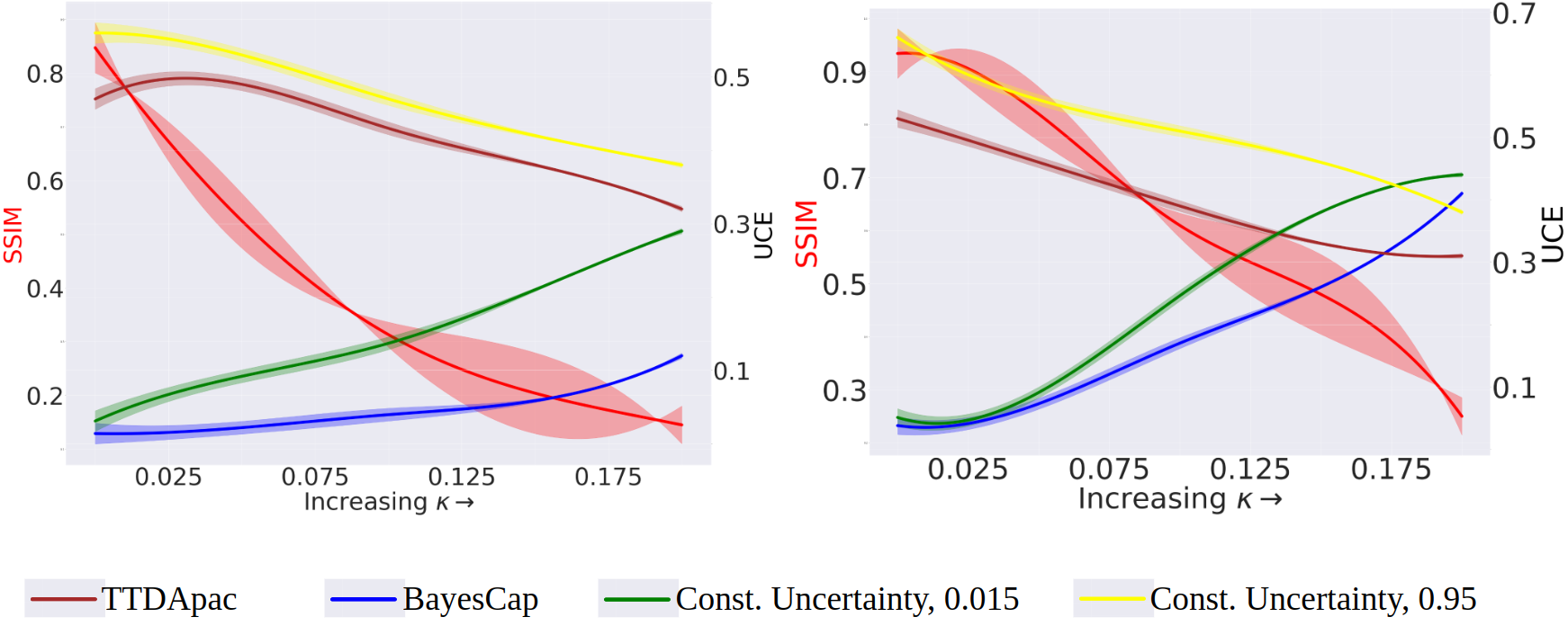
Figure 1: Impact of the identity mapping. Degrading the quality of the identity mapping (SSIM) at inference, leads to poorly calibrated uncertainty (UCE). $\kappa$ represents the magnitude of noise used for degrading the identity mapping. (Left) super-resolution on set5 dataset and (Right) Deblurring on GoPro dataset.

We notice that, at the beginning when the input samples are not degraded the UCE for TTDApac is very high, this happens because the TTDApac leads to an uncertainty map that already has a very high value at every pixel and is not in agreement with the lower per-pixel error (between the prediction and the groundtruth) as evident from Figure 4 and 5 in the main manuscript. As the input sample becomes more noisy (i.e., increasing $\kappa$), the quality of the predictions degrade sharply leading to higher error values, whereas the uncertainty values obtained using TTDApac do not change much. This leads to better agreement between the high error and the uncertainty values causing UCE to decrease with increasing $\kappa$. Moreover, this also indicates that TTDApac does not provide well-calibrated uncertainty estimates. To shed more light on this phenomena, we also study the UCE trend for two more baseline tasks, where the uncertainty maps are set to constants (0.015 and 0.95). For a low-value constant (0.015) uncertainty map, as we degrade the input samples, the quality of output prediction also deteriorates and the disagreement between per-pixel uncertainty and error increases, leading to higher UCE values, therefore there is an increasing UCE trend. For a high-value constant (0.95) uncertainty map, as we degrade the input samples, the quality of output prediction also deteriorates leading to higher error values which are also closer to higher values of per-pixel uncertainty, leading to more agreement between uncertainty and error and lower UCE values, therefore there is a decreasing UCE trend. Note that this does not indicate well-calibrated uncertainty estimates. This phenomena is observed for both the super-resolution (Figure 1-Left) and deblurring (Figure 1-Right).

1.2 Necessity of the Identity Mapping Term.

We ablate our BayesCap by removing the identity mapping loss, i.e., by using the following loss to train BayesCap

$$\phi^{*}=\underset{\phi}{\text{argmin}}\sum_{i=1}^{i=N}\underbrace{\left(\frac{|\tilde{\mathbf{y}}_{i}-\mathbf{y}_{i}|}{\tilde{\alpha}_{i}}\right)^{\tilde{\beta}_{i}}-\log\frac{\tilde{\beta}_{i}}{\tilde{\alpha}_{i}}+\log\Gamma(\frac{1}{\tilde{\beta}_{i}})}_{\text{Negative log-likelihood}}$$

and compare it with SRGAN on the BSD100 dataset for image super-resolution. Our results 0.34/0.028 UCE score and 0.23/0.45 C.Coeff (for ablation/BayesCap resp.) indicate that the identity mapping is essential to learn the calibrated uncertainties.

Model	UCE	C.Coeff
No Idenity Mapping	0.34	0.23
BayesCap	0.028	0.45

Table 1: Ablation study for the task of image super-resolution with and without the identity mapping.

1.3 Comparison with Generalized Gaussian Scratch Model.

Scratch is the model trained from scratch that corresponds to Kendall et al. [kendall2017uncertainties]. For completeness, we also perform experiments with Scratch model modified to predict the parameters of the Generalized Gaussian distribution, where the fidelity loss term is given by the following equation,

$$\mathcal{L}_{\text{fidelity}}=\sum_{i=1}^{i=N}\left(\frac{|\hat{\mathbf{y}}_{i}-\mathbf{y}_{i}|}{\hat{\alpha}_{i}}\right)^{\hat{\beta}_{i}}-\log\frac{\hat{\beta}_{i}}{\hat{\alpha}_{i}}+\log\Gamma(\frac{1}{\hat{\beta}_{i}})+\lambda_{1}*\mathcal{L}_{\text{content}}$$

where, $\mathcal{L}_{\text{content}}$ is the content loss from [Ledig_2017_CVPR] and the total loss function used for training the network is given by

$$\mathcal{L}_{\text{total}}=\lambda_{2}\mathcal{L}_{\text{fidelity}}+\lambda_{3}\mathcal{L}_{\text{adversarial}}$$

Where $\mathcal{L}_{\text{adversarial}}$ is given by,

$$\mathcal{L}_{\text{adversarial}}=\sum_{j=1}^{j=M}-\log{D_{\theta_{D}}({G_{\theta_{G}}(x^{j}))}}$$

where, $x^{j}$ represents $j^{th}$ image and $M$ is the total number of images in the dataset. For super-resolution on the BSD100 dataset, the following are the results:

Model	PSNR	UCE
GGD-Scratch	24.78	0.033
Scratch	24.39	0.057
BayesCap	25.16	0.028

Table 2: Additional model for the task of image super-resolution that models output as Generalized Gaussian Distribution (GGD)

1.4 Effect of Post-Hoc Calibration Methods.

We apply post-hoc calibration (variance scaling) from [laves2020calibration], that is, we find the optimal scale ($s^{*}$) by optimizing,

$$s^{*}=\underset{s}{\text{argmin }}N\log(s)+\frac{1}{s^{2}}\sum_{i=1}^{N}\frac{|\hat{\mathbf{y}}_{i}-\mathbf{y}_{i}|^{2}}{\hat{\sigma_{i}}^{2}}$$

We then rescale the derived variances using the optimal scale ($s^{*}$). We find that the calibration of other models remains worse compared to our BayesCap as shown in the following for super-resolution task on BSD100:

Model	UCE	C.Coeff
Scratch	0.036	0.41
BayesCap	0.028	0.45

Table 3: Variance scaling for post hoc uncertainty calibration for the task of image super-resolution

1.5 Additional Metrics for Calibration.

We additionally include the Expected Calibration Error (ECE), Sharpness and Negative Log Likelihood (NLL) metrics comparing our BayesCap with Scratch and DO respectively for image super-res. on BSD100 to measure calibration of the uncertainties [zhou2020estimating, chung2021beyond], as shown below:

Model	ECE	Sharpness	NLL
BayesCap	0.83	1.65	0.21
Scratch	1.26	2.55	0.35
DO	4.47	8.41	0.47

Table 4: Additional metrics for uncertainty calibration for the task of image super-resolution

2 Application: Out-of-Distribution Analysis

In the main paper, we provide an application for the derived uncertainties from our method to detect OOD samples in depth estimation task. We used a model trained with KITTI dataset (i.e., MonoDepth2) and evaluate the model on data from KITTI test set (i.e., in distribution), test set for Indian Driving dataset (i.e., out of distribution), and also on test set of Places365 dataset (i.e., severely out of distribution). We used the following methods to detect OOD samples.

Using pretrained features for OOD detection. We computed the mean features for the KITTI validation set images using the feature extracted from the intermediate layer of pretrained MonoDepth2 model, say $\mathscr{M}$, with intermediate feature represented by $\mathscr{M}_{l}(\cdot)$ (shown below),

$$\mathcal{F}_{\text{mean}}=\frac{1}{|\text{KITTI val}|}\sum_{i=1}^{i=|\text{KITTI val}|}\mathscr{M}_{l}(x_{i})\text{ }\forall x_{i}\in\text{KITTI val}$$ (1)

Then, at inference we extract the same intermediate feature for the image being analysed and compute the L2 distance between the KITTI validation set mean feature and the features of the analysed images.

$$f_{t}=\mathscr{M}_{l}(x_{t})\text{ }\forall x_{t}\in\text{Inference set}$$ (2)

$$d_{t}=||f_{t}-\mathcal{F}_{\text{mean}}||^{2}$$ (3)

$$\text{is }x_{t}\text{ OOD?}=\begin{cases}\text{True},&\text{if }d_{t}\geq\tau\\ \text{False},&d_{t}<\tau\end{cases}$$ (4)

Using autoencoder features for OOD detection. We computed the mean features for the KITTI validation set images using the feature extracted from the bottleneck layer of the autoencoder (say $\mathscr{A}$, with bottleneck feature represented by $\mathscr{A}_{b}(\cdot)$) trained on top of a pretrained MonoDepth2 model, i.e.,

$$\mathcal{F}_{\text{mean}}=\frac{1}{|\text{KITTI val}|}\sum_{i=1}^{i=|\text{KITTI val}|}\mathscr{A}_{b}(\mathscr{M}(x_{i}))\text{ }\forall x_{i}\in\text{KITTI val}$$ (5)

Then, at inference we extract the same bottleneck feature for the image being analysed and compute the L2 distance between the KITTI validation set mean feature and the features of the analysed images.

$$f_{t}=\mathscr{A}_{b}(\mathscr{M}(x_{t}))\text{ }\forall x_{t}\in\text{Inference set}$$ (6)

$$d_{t}=||f_{t}-\mathcal{F}_{\text{mean}}||^{2}$$ (7)

$$\text{is }x_{t}\text{ OOD?}=\begin{cases}\text{True},&\text{if }d_{t}\geq\tau\\ \text{False},&d_{t}<\tau\end{cases}$$ (8)

Using mean uncertainty for OOD detection. At inference, we computed the mean uncertainty values for the images in the inference set using the BayesCap (say $\mathscr{B}$, with uncertainty map represented by $\mathscr{B}_{u}$) trained on top of pretrained MonoDepth2 model, and use that to decide if a sample is OOD, i.e.,

$$u_{t}=\text{mean}(\mathscr{B}_{u}(\mathscr{M}(x_{t})))\text{ }\forall x_{t}\in\text{Inference set}$$ (9)

$$\text{is }x_{t}\text{ OOD?}=\begin{cases}\text{True},&\text{if }u_{t}\geq\tau\\ \text{False},&u_{t}<\tau\end{cases}$$ (10)