On the Approximation of Unbounded Convex Sets by Polyhedra

Abstract

This article is concerned with the approximation of unbounded convex sets by polyhedra. While there is an abundance of literature investigating this task for compact sets, results on the unbounded case are scarce. We first point out the connections between existing results before introducing a new notion of polyhedral approximation called $\left(\varepsilon,\delta\right)$-approximation that integrates the unbounded case in a meaningful way. Some basic results about $\left(\varepsilon,\delta\right)$-approximations are proven for general convex sets. In the last section an algorithm for the computation of $\left(\varepsilon,\delta\right)$-approximations of spectrahedra is presented. Correctness and finiteness of the algorithm are proven.

1 Introduction

The problem of approximating a convex set $C$ by a polyhedron in the Hausdorff distance has been studied systematically for at least a century [27] and has a variety of applications in mathematical programming. These include algorithms for convex optimization problems that approximate the feasible region by a sequence of polyhedra [4, 20] or solution concepts for convex vector optimization problems [32, 10, 24]. Moreover, there are multiple algorithms for mixed-integer convex optimzation problems that are based on polyhedral outer approximations, see [7, 39, 22]. Interest in this problem is fueled by the fact that polyhedra have a simple structure in the sense that they can be described by finitely many points and directions. This finite structure makes computations with polyhedra more viable than with general convex sets. Hence, it is desirable to work with polyhedra that approximate some complicated set well. If the set $C$ to be approximated is assumed to be compact, then numerous theoretical results are available. This includes asymptotic [11, 33] and explicit [3] bounds on the number of vertices that a polyhedron needs to have in order to approximate $C$ to within a prescribed accuracy. Moreover, iterative algorithms, so called augmenting and cutting schemes, for the polyhedral approximation of convex bodies are known, see [17]. Some convergence properties are discussed in [18] and [19]. An overview about combinatorial aspects of the approximation of convex bodies is collected in the survey article by Bronshteĭn [2].

If boundedness of the set $C$ is not assumed, the amount of literature on the problem is scarce, although there are various applications where unbounded convex sets arise naturally. In convex vector optimization, for example, it is known that the so-called extended feasible image or upper image contains the set of nondominated points on its boundary, see e.g. [23, 10]. Due to its geometric properties it is advantageous to work with this unbounded set instead of with the feasible image itself. Another application is in large deviations theory, which, generally speaking, is the study of the asymptotic behaviour of tails of sequences of probability distributions, see [37]. Under certain conditions bounds for this behaviour can be obtained in terms of rate functions of probability distributions. In [29] such bounds are obtained under the condition that the level sets of a specific convex rate function can be approximated by polyhedra. Moreover, the authors of [26] generalize the algorithm in [7] and consider mixed-integer convex optimization problems, whose feasible region is not necessarily bounded. The problems are solved by computing polyhedral outer approximations of the feasible region in such a fashion that reaching a globally optimal solution is guaranteed.

The most notable result about the polyhedral approximation of $C$ is due to Ney and Robinson [29] who give a characterization of the class of sets that can be approximated arbitrarily well by polyhedra in the Hausdorff distance. However, this class is relatively small as restrictive assumptions on the recession cone of $C$ have to be made, such as polyhedrality. The reason boils down to the fact that the Hausdorff distance is seldom suitable to measure the similarity between unbounded sets. In fact, the Hausdorff distance between closed and convex sets is finite only if the recession cones of the sets are equal, see Proposition 3.5 in Section 3. Due to this difficulty, additional assumptions about the structure of the problem have to be made in each of the aforementioned applications. These include polyhedrality of the ordering cone or boundedness of the problem in convex vector optimization, see e.g. [24, 8], polyhedrality of a cone generated by the rate function in large deviations theory, or strong duality when dealing with convex optimization problems. In 2018, Ulus [36] characterized the tractability of convex vector optimization problems in terms of polyhedral approximations. One important necessary condition is the so-called self-boundedness of the problem.

Considering the facts mentioned, polyhedral approximation of unbounded convex sets requires a notion that does not solely rely on the Hausdorff distance. To this end our main contribution is the introduction of the notion of $\left(\varepsilon,\delta\right)$-approximation for closed convex sets $C$ that do not contain lines. One feature of $\left(\varepsilon,\delta\right)$-approximations is that the recession cones of the involved sets play an important role. We show that $\left(\varepsilon,\delta\right)$-approximations define a meaningful notion of polyhedral approximation in the sense that a sequence of approximations converges to the set $C$ as $\varepsilon$ and $\delta$ diminish. This convergence is achieved in the sense of Painlevé-Kuratowski, who define convergence for sequences of sets, see [31]. Moreover, we present an algorithm for the computation of $\left(\varepsilon,\delta\right)$-approximations when the set $C$ is a spectrahedron, i.e. defined by a linear matrix inequality. We also prove correctness and finiteness of the algorithm. Its main purpose, however, is to show that $\left(\varepsilon,\delta\right)$-approximations can be constructed in finitely many steps theoretically.

This article is organized as follows. In the next section we introduce the necessary notation and provide definitions. In Section 3 we compare the results by Ney and Robinson [29] with the results by Ulus [36] and put them in relation. In particular, we show that self-boundedness is a special case of the property that the excess of a set over its own recession cone is finite. The concept of $\left(\varepsilon,\delta\right)$-approximations is introduced in Section 4. We prove a bound on the Hausdorff distance between truncations of an $\left(\varepsilon,\delta\right)$-approximation and truncations of $C$. The main result is Theorem 4.9. It states that a sequence of $\left(\varepsilon,\delta\right)$-approximations of $C$ converges to $C$ in the sense of Painlevé-Kuratowski as $\varepsilon$ and $\delta$ tend to zero. In the last section we present the aforementioned algorithm and prove correctness and finiteness as well as illustrate it with two examples.

2 Preliminaries

Throughout this article we denote by $\operatorname{cl}C$, $\operatorname{int}C$, $0^{+}{C}$, $\operatorname{conv}C$, and $\operatorname{cone}C$ the closure, interior, recession cone, convex hull and conical hull of a set $C$, respectively. A compact convex set with nonempty interior is called a convex body. The Euclidean ball with radius $r$ centered at a point ${c\in\mathbb{R}^{n}}$ is denoted by $B_{r}(c)$. A point $c$ of a convex set $C$ is called an extreme point of $C$, if $C\setminus\{c\}$ is convex. The set of extreme points of $C$ is denoted by $\operatorname{ext}C$. Extreme points are exactly the points of $C$ that cannot be written as a proper convex combination of elements of $C$ [30, p. 162]. For finite sets $V,D\subseteq\mathbb{R}^{n}$, the set

$$P=\operatorname{conv}V+\operatorname{cone}D$$ (1)

is called a polyhedron. The plus sign denotes Minkowski addition. The sets $V,D$ in (1) are called a $V$-representation of $P$ as it is expressed in terms of its vertices and directions. A polyhedron can equivalently be expressed as a finite intersection of closed halfspaces [30, Theorem 19.1], i.e.

$$P=\{x\in\mathbb{R}^{n}\mid Ax\leq b\}$$ (2)

for a matrix $A\in\mathbb{R}^{m\times n}$ and a vector $b\in\mathbb{R}^{m}$. The data $(A,b)$ are called a $H$-representation of $P$. The extreme points of a polyhedron $P$ are called vertices of $P$ and are denoted by $\operatorname{vert}P$. For symmetric matrices $A_{0},A_{1},\dots,A_{n}$ of arbitrary fixed size we define

$$\bar{\mathcal{A}}(x):=\sum_{i=1}^{n}x_{i}A_{i}\quad\text{and}\quad\mathcal{A}(x):=\bar{\mathcal{A}}(x)+A_{0},$$ (3)

i.e. a linear combination of the $A_{i}$ and a translation of $\bar{\mathcal{A}}(x)$ by $A_{0}$, respectively. We denote by $A\succ 0$ ($A\succcurlyeq 0$) positive (semi-)definiteness of the symmetric matrix $A$. A set of the form $\{x\in\mathbb{R}^{n}\mid\mathcal{A}(x)\succcurlyeq 0\}$ is called a spectrahedron. Spectrahedra are a generalization of polyhedra for which many geometric properties of polyhedra generalize nicely, e.g. the recession cone of a spectrahedron $C$ is obtained as $\{x\in\mathbb{R}^{n}\mid\bar{\mathcal{A}}(x)\succcurlyeq 0\}$, see [13], whereas the recession cone of a polyhedron in $H$-representation is $\{x\in\mathbb{R}^{n}\mid Ax\leq 0\}$. Given a cone $K$ the set ${K}^{\circ}=\{y\in\mathbb{R}^{n}\mid\forall x\in K:x^{\mathsf{T}}y\leq 0\}$ is called the polar cone of $K$. The polar ${(0^{+}{C})}^{\circ}$ of the recession cone of a spectrahedron $C$ is computed as

$${(0^{+}{C})}^{\circ}=\operatorname{cl}\left\{\left(-A_{1}\cdot X,\dots,-A_{n}\cdot X\right)^{\mathsf{T}}\mid X\succcurlyeq 0\right\},$$ (4)

where $A_{i}\cdot X$ means the trace of the matrix product $A_{i}X$, see [13, Section 3]. A cone $K$ is called polyhedral if ${K=\operatorname{cone}D}$ for some finite set $D$ and pointed if ${K\cap(-K)=\{0\}}$. A set whose recession cone is pointed is called line-free. It is well known, that a closed convex set contains an extreme point if and only if it is line-free, see [30, Corollary 18.5.3]. Given nonempty sets ${C_{1},C_{2}\subseteq\mathbb{R}^{n}}$ the excess of $C_{1}$ over $C_{2}$, ${e[{C_{1}},{C_{2}}]}$, is defined as

$$e[{C_{1}},{C_{2}}]=\adjustlimits{\sup}_{c_{1}\in C_{1}}{\inf}_{c_{2}\in C_{2}}\left\lVert{c_{1}-c_{2}}\right\rVert,$$ (5)

where $\left\lVert{\cdot}\right\rVert$ denotes the Euclidean norm. The Hausdorff distance between $C_{1}$ and $C_{2}$, ${d_{\mathsf{H}}\left({C_{1}},{C_{2}}\right)}$, is then expressed as

$$d_{\mathsf{H}}\left({C_{1}},{C_{2}}\right)=\max\{e[{C_{1}},{C_{2}}],e[{C_{2}},{C_{1}}]\}.$$ (6)

It is well known, that the Hausdorff distance defines a metric on the space of nonempty compact subsets of $\mathbb{R}^{n}$. Between unbounded sets the Hausdorff distance may be infinite. A polyhedron $P$ is called an $\varepsilon$-approximation of a convex set $C$ if $d_{\mathsf{H}}\left({P},{C}\right)\leq\varepsilon$.

3 Polyhedral Approximation in the Hausdorff Distance

Every convex body can be approximated arbitrarily well by a polytope in the Hausdorff distance, see e.g. [33]. Moreover, algorithms for the computation of $\varepsilon$-approximations exist for which the convergence rate is known [17]. For the approximation of unbounded convex sets only the following theorem is known, which provides a characterization of the sets that can be approximated by polyhedra in the Hausdorff distance.

Theorem 3.1 (see [29, Theorem 2.1]).

Let $C\subseteq\mathbb{R}^{n}$ be nonempty and closed. Then the following are equivalent:

1. $C$ is convex, $0^{+}{C}$ is polyhedral, and $e[{C},{0^{+}{C}}]<+\infty$.

2. There exists a polyhedral cone $K$ such that for every $\varepsilon>0$ there exists a finite set $V\subseteq\mathbb{R}^{n}$ such that ${d_{\mathsf{H}}\left({\operatorname{conv}V+K},{C}\right)\leq\varepsilon}$.

Further, if (ii) holds then $K=0^{+}{C}$.

A related result is found in [36], where the approximate solvability of convex vector optimization problems in terms of polyhedral approximations is investigated. In order to state the result and establish the relationship to Theorem 3.1 we need the following definition from [36].

Definition 3.2.

A set $C\subsetneq\mathbb{R}^{n}$, with a nontrivial recession cone is called self-bounded, if there exists $y\in\mathbb{R}^{n}$ such that ${\{y\}+0^{+}{C}\supseteq C}$.

Adjusted to our notation, the mentioned result can be stated as:

Proposition 3.3 (see [36, Proposition 3.7]).

Let $C\subseteq\mathbb{R}^{n}$ be closed and convex. If $C$ is self-bounded, then there exists a finite set $V\subseteq\mathbb{R}^{n}$ such that ${d_{\mathsf{H}}\left({\operatorname{conv}V+0^{+}{C}},{C}\right)\leq\varepsilon}$.

If $0^{+}{C}$ is polyhedral, then, clearly, $C$ can be approximated by a polyhedron. The difference to Theorem 3.1 is the self-boundedness of $C$ instead of the finiteness of ${e[{C},{0^{+}{C}}]}$. The following theorem points out the connection between these conditions and shows, that under an additional assumption, both coincide. The relationships are illustrated in Figure 1.

Theorem 3.4.

Given a nonempty, closed and convex set $C\subseteq\mathbb{R}^{n}$, consider the statements

1. $e[{C},{0^{+}{C}}]<+\infty$,

2. $C$ is self-bounded,

3. There is a compact set $K\subseteq\mathbb{R}^{n}$ such that ${K+0^{+}{C}\supseteq C}$.

Then the following implications are true: (i) $\Leftrightarrow$ (iii) and (ii) $\Rightarrow$ (iii). If, additionally, $0^{+}{C}$ is solid, then (i) – (iii) are equivalent.

Proof.

We start with the assertion (i) $\Rightarrow$ (iii). Let ${M=e[{C},{0^{+}{C}}]}$, ${c\in C}$ be arbitrary and ${r_{c}\in 0^{+}{C}}$ such that ${\left\lVert{c-r_{c}}\right\rVert=\inf_{r\in 0^{+}{C}}\left\lVert{c-r}\right\rVert}$. This infimum is uniquely attained, because $0^{+}{C}$ is closed and convex. Then ${\left\lVert{c-r_{c}}\right\rVert\leq M}$ and we conclude ${c=(c-r_{c})+r_{c}\in B_{M}(0)+0^{+}{C}}$. Therefore, ${B_{M}(0)+0^{+}{C}\supseteq C}$.

To show (iii) $\Rightarrow$ (i), let ${K+0^{+}{C}\supseteq C}$ for some compact set $K$. Then we have

$$e[{C},{0^{+}{C}}] \leq e[{K+0^{+}{C}},{0^{+}{C}}]$$

$$=\adjustlimits{\sup}_{\begin{subarray}{c}k\in K\\ r\in 0^{+}{C}\end{subarray}}{\inf}_{\bar{r}\in 0^{+}{C}}\left\lVert{(k+r)-\bar{r}}\right\rVert$$

$$\leq\sup_{\begin{subarray}{c}k\in K\\ r\in 0^{+}{C}\end{subarray}}\left\lVert{(k+r)-r}\right\rVert$$

$$=\sup_{k\in K}\left\lVert{k}\right\rVert<+\infty.$$

The implication (ii) $\Rightarrow$ (iii) is trivial with ${K=\{y\}}$. For the last part we show (iii) $\Rightarrow$ (ii), assuming $0^{+}{C}$ is solid. If ${e[{C},{0^{+}{C}}]=0}$, then ${C\subseteq 0^{+}{C}}$ and we can set ${y=0}$. Now, let ${e[{C},{0^{+}{C}}]=M>0}$ and fix ${c\in\operatorname{int}C}$. Then there exists ${\varepsilon>0}$ such that ${B_{\varepsilon}(c)\subseteq 0^{+}{C}}$. We have

$$B_{M}\left(\frac{M}{\varepsilon}c\right) =\frac{M}{\varepsilon}B_{\varepsilon}(c)$$

$$\subseteq\frac{M}{\varepsilon}0^{+}{C}$$

$$=0^{+}{C}.$$

Therefore, ${\left\{-\frac{M}{\varepsilon}c\right\}+0^{+}{C}\supseteq B_{M}(0)}$ and, since $0^{+}{C}$ is convex, $\left\{-\frac{M}{\varepsilon}c\right\}+0^{+}{C}\supseteq B_{M}(0)+0^{+}{C}$. From the first part of the proof we know, that ${B_{M}(0)+0^{+}{C}\supseteq C}$, which completes the proof. ∎

 

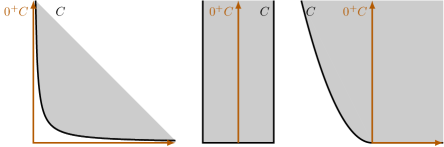
Figure 1: Illustration of Theorem 3.4. Left: The set $C$ is contained in its own recession cone. Therefore, it is self-bounded and $e[{C},{0^{+}{C}}]=0$. Center: The excess of $C$ over its recession cone is finite and attained in any of the two vertices. However, $C$ is not self-bounded, because it cannot be contained in a translation of $0^{+}{C}$. Right: A set that is neither self-bounded nor does it hold $e[{C},{0^{+}{C}}]<\infty$. Traversing the parabolic arc, the distance to $0^{+}{C}$ grows without bound.

Example 3.1.

To see that ${e[{C},{0^{+}{C}}]<+\infty}$ does not imply self-boundedness of $C$ unless $0^{+}{C}$ is solid, consider the following counterexample. In $\mathbb{R}^{2}$ let ${C=\operatorname{conv}\{\pm e_{1}\}+\operatorname{cone}\{e_{2}\}}$, where $e_{i}$ denotes the $i$-th unit vector. Then one has the equality $e[{C},{0^{+}{C}}]=1$, but $C$ is not self-bounded. The set is illustrated in the center of Figure 1.

In view of the above result, we suggest calling a set self-bounded, if it satisfies Property (iii). On one hand, this extends the notion to sets whose recession cone is not solid. And on the other hand, makes every compact set self-bounded, rather than just singletons. Since in [36] cones are assumed to be solid, Theorem 3.4 proves that a convex vector optimization problem is tractable in terms of polyhedral approximations, if and only if the upper image [36, Equation 6] of the problem satisfies (i) in Theorem 3.1.

The reason that many unbounded convex sets are beyond the scope of polyhedral approximation in the Hausdorff distance is that it is by nature designed to behave nicely only for compact sets. The following proposition specifies this.

Proposition 3.5.

For closed and convex sets $C_{1},C_{2}\subseteq\mathbb{R}^{n}$ it is true, that $d_{\mathsf{H}}\left({C_{1}},{C_{2}}\right)<+\infty$ only if ${0^{+}{C_{1}}=0^{+}{C_{2}}}$.

Proof.

Assume ${0^{+}{C_{1}}\neq 0^{+}{C_{2}}}$ and let w.l.o.g. ${r\in 0^{+}{C_{1}}\setminus 0^{+}{C_{2}}}$. Consider the equivalent definition of the Hausdorff distance:

$$d_{\mathsf{H}}\left({C_{1}},{C_{2}}\right)=\inf\left\{\varepsilon>0\mid C_{1}\subseteq C_{2}+B_{\varepsilon}(0),C_{2}\subseteq C_{1}+B_{\varepsilon}(0)\right\}.$$

Let $\varepsilon$ be large enough such that ${C_{1}\cap\left(C_{2}+B_{\varepsilon}(0)\right)\neq\emptyset}$ and let $z$ be an element of this set. Then ${z+\mu r\in C_{1}}$ for all ${\mu\geq 0}$. The recession cone of ${C_{2}+B_{e}(0)}$ is $0^{+}{C_{2}}$ according to [30, Proposition 9.1.2]. Therefore, there exists some $\mu_{\varepsilon}$ such that ${z+\mu r\notin C_{2}+B_{e}(0)}$ for all ${\mu\geq\mu_{\varepsilon}}$. This yields ${d_{\mathsf{H}}\left({C_{1}},{C_{2}}\right)\geq\varepsilon}$ and the claim follows with ${\varepsilon\to\infty}$. ∎

4 A Polyhedral Approximation Scheme for Closed Convex Line-Free Sets

We have seen that, in order to approximate a set $C$ by a polyhedron $P$ in the Hausdorff distance, their recession cones need to be identical. Theorems 3.1 and 3.4 tell us that this is achievable only for specific sets $C$. To treat a larger class of sets, a concept is needed that quantifies similarity between closed convex cones, similar to how the Hausdorff distance quantifies similarity between compact sets.

Definition 4.1.

Given nonempty closed convex cones ${K_{1},K_{2}\subseteq\mathbb{R}^{n}}$, the truncated Hausdorff distance between $K_{1}$ and $K_{2}$, ${\bar{d}_{\mathsf{H}}(K_{1},K_{2})}$, is defined as

$$\bar{d}_{\mathsf{H}}(K_{1},K_{2}):=d_{\mathsf{H}}\left({K_{1}\cap B_{1}(0)},{K_{2}\cap B_{1}(0)}\right).$$ (7)

Since every cone contains the origin, it is immediate that ${\bar{d}_{\mathsf{H}}(K_{1},K_{2})\leq 1}$. The truncated Hausdorff distance defines a metric on the set of closed convex cones in $\mathbb{R}^{n}$, see [14]. However, it is only one way among many to measure the distance between convex cones. We suggest the survey in [16] for a more thorough discussion of the topic. With the truncated Hausdorff distance we define the following notion of polyhedral approximation of convex sets that are not necessarily bounded.

Definition 4.2.

Given a nonempty closed convex and line-free set ${C\subseteq\mathbb{R}^{n}}$, a line-free polyhedron $P$ is called an ${\left(\varepsilon,\delta\right)}$-approximation of $C$ if

1. $e[{\operatorname{vert}P},{C}]\leq\varepsilon$,

2. $\bar{d}_{\mathsf{H}}(0^{+}{P},0^{+}{C})\leq\delta$,

3. $P\supseteq C$.

 

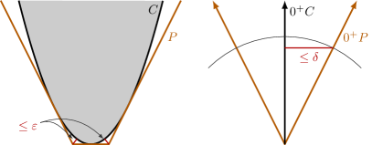
Figure 2: Left: The polyhedron $P$ is an $\left(\varepsilon,\delta\right)$-approximation of the grey set $C$. Right: The recession cones of the sets on the left. The truncated Hausdorff distance between them is at most $\delta$.

Remark 4.3.

The assumption that $P$ is line-free is equivalent to $\operatorname{vert}P\neq\emptyset$ and hence required for condition (i) in the definition. Condition (iii) means that $P$ is an outer approximation of $C$. This is required, because otherwise the roles of $P$ and $C$ would have to be interchanged in (i). However, it is not clear how to proceed with this in a meaningful fashion. The analogue of considering vertices of $P$ would be to consider extreme points of $C$ instead. The set of extreme points of $C$ may be unbounded and it is in general not possible to enforce the upper bound of $\varepsilon$. Lastly, we decided to make a distinction between $\varepsilon$ and $\delta$, because scales of these error measures may be very different depending on the sets, i.e. $\delta$ is always bounded from above by 1, but for $\varepsilon$ it may be useful to allow values larger than 1.

Figure 2 illustrates the definition. We will show that an $\left(\varepsilon,\delta\right)$-approximation of a set $C$ approximates $C$ in a meaningful way. To this end, we consider the Painlevé-Kuratowski convergence, a notion of set convergence that is suitable for a broader class of sets than convergence with respect to the Hausdorff distance.

Definition 4.4.

A sequence $\{C^{\nu}\}_{\nu\in\mathbb{N}}$ of subsets of $\mathbb{R}^{n}$ is said to converge to ${C\subseteq\mathbb{R}^{n}}$ in the sense of Painlevé-Kuratowski, denoted by ${C^{\nu}\rightarrow C}$, if the following equalities hold:

$$C =\left\{x\in\mathbb{R}^{n}\middle|\begin{matrix}\text{for all open neighbourhoods }U\text{ of }x,\\ U\cap C^{\nu}\neq\emptyset\text{ for large enough }\nu\end{matrix}\right\}$$

$$=\left\{x\in\mathbb{R}^{n}\middle|\begin{matrix}\text{for all open neighbourhoods }U\text{ of }x,\\ U\cap C^{\nu}\neq\emptyset\text{ for infinitely many }\nu\end{matrix}\right\}.$$

To conserve space and enhance readability we will denote by $C^{\nu}$ the sequence $\{C^{\nu}\}_{\nu\in\mathbb{N}}$ as well as the specific element $C^{\nu}$ of this sequence whenever there is no ambiguity. The two sets in the definition are called the inner and outer limit of $C^{\nu}$, respectively. Convergence in the sense of Painlevé-Kuratowski is weaker than convergence in the Hausdorff distance, but both concepts coincide when restricted to compact subsets, see Example 4.1 and [31, pp. 131–138]. However, for convex sets Painlevé-Kuratowski convergence can be characterized using the Hausdorff distance.

Example 4.1 (see [31, p. 118]).

Consider the sequence of sets for which $C^{\nu}=\left\{{x,y^{\nu}}\right\}$ for $x,y^{\nu}\in\mathbb{R}^{n}$ and $\left\lVert{y^{\nu}}\right\rVert\rightarrow\infty$. Then $C^{\nu}$ converges in the sense of Painlevé-Kuratowski to the singleton $C=\left\{{x}\right\}$, but does not converge in the Hausdorff distance, because $d_{\mathsf{H}}\left({C^{\nu}},{C}\right)=\left\lVert{x-y^{\nu}}\right\rVert\rightarrow\infty$.

Theorem 4.5 (see [31, p. 120]).

A sequence $C^{\nu}$ of nonempty closed and convex sets converges to $C$ in the sense of Painlevé-Kuratowski if and only if there exist $x\in\mathbb{R}^{n}$ and $r_{0}\in\mathbb{R}$, such that for all $r\geq r_{0}$ it holds, that

$$d_{\mathsf{H}}\left({C^{\nu}\cap B_{r}(x)},{C\cap B_{r}(x)}\right)\rightarrow 0.$$ (8)

In geometric terms this means that a sequence of nonempty closed and convex sets converges in the sense of Painlevé-Kuratowski if and only if it converges in the Hausdorff distance on every nonempty compact subset. In the remainder of this section we show that $\left(\varepsilon,\delta\right)$-approximations provide a meaningful notion of polyhedral approximation for unbounded sets in the sense that a sequence of approximations converges as defined in Definition 4.2 if $\varepsilon$ and $\delta$ tend to zero. To this end we need some preparatory results. The first one yields a bound on the Hausdorff distance between truncations of a set and truncations of an $\left(\varepsilon,\delta\right)$-approximation.

Proposition 4.6.

Let $C\subseteq\mathbb{R}^{n}$ be nonempty closed convex and line-free and let $P$ be an $\left(\varepsilon,\delta\right)$-approximation of $C$. Then for every $x\in\operatorname{conv}\operatorname{vert}P$ and $r\geq\varepsilon$ it holds true, that

$$d_{\mathsf{H}}\left({P\cap B_{r}(x)},{C\cap B_{r}(x)}\right)\leq 2\left(\varepsilon+\delta\left(r+\left\lVert{x-v}\right\rVert\right)\right)$$ (9)

for some $v\in\operatorname{conv}\operatorname{vert}P$. In particular, if $d_{\mathsf{H}}\left({P\cap B_{r}(x)},{C\cap B_{r}(x)}\right)$ is attained as $\left\lVert{p-c}\right\rVert$ with $p\in P$, then $p=v+td$ for some $d\in 0^{+}{P}$ and $t\geq 0$.

Proof.

Denote by $\bar{P}$, $\bar{C}$, and $V$, $P\cap B_{r}(x)$, $C\cap B_{r}(x)$, and $\operatorname{conv}\operatorname{vert}P$, respectively. Since $\bar{P},\bar{C}$ are nonempty convex and compact, $d_{\mathsf{H}}\left({\bar{P}},{\bar{C}}\right)=\left\lVert{p^{*}-c^{*}}\right\rVert$ for some $p^{*}\in\bar{P}$ and $c^{*}\in\bar{C}$. For $\lambda\in[0,1]$ let $z(\lambda)=\lambda p^{*}+(1-\lambda)x$. We distinguish two cases. First, assume $p^{*}\in V$. Then $z(\lambda)\in V$ for every ${\lambda\in[0,1]}$ and, due to (i) in Definition 4.2, there is ${c_{\lambda}\in\bar{C}}$ with ${\left\lVert{z(\lambda)-c_{\lambda}}\right\rVert\leq\varepsilon}$. If $\left\lVert{p^{*}-x}\right\rVert\leq\varepsilon$ then

$$\left\lVert{p^{*}-c^{*}}\right\rVert\leq\left\lVert{p^{*}-c_{0}}\right\rVert\leq\left\lVert{p^{*}-x}\right\rVert+\left\lVert{x-c_{0}}\right\rVert\leq 2\varepsilon.$$

If $\left\lVert{p^{*}-x}\right\rVert>\varepsilon$, set ${\lambda}^{*}=\frac{\varepsilon}{\left\lVert{p^{*}-x}\right\rVert}$. Similarly, we have

$$\left\lVert{p^{*}-c^{*}}\right\rVert\leq\left\lVert{p^{*}-c_{{\lambda}^{*}}}\right\rVert\leq\left\lVert{p^{*}-z({\lambda}^{*})}\right\rVert+\left\lVert{z({\lambda}^{*})-c_{{\lambda}^{*}}}\right\rVert\leq 2\varepsilon.$$

Now, assume ${p^{*}\notin V}$. Then there exists $\bar{\lambda}\in(0,1)$, such that $z(\bar{\lambda})\in V$ and $z(\lambda)\notin V$ for all $\lambda\in(\bar{\lambda},1]$. For ${\lambda\in(\bar{\lambda},1]}$, $z(\lambda)$ can be written as ${z(\lambda)=v_{\lambda}+t_{\lambda}d_{\lambda}}$ with $v_{\lambda}=\operatorname{argmin}\{\left\lVert{z(\bar{\lambda})-v}\right\rVert\;\mid\;$ $v\in\left(\{z(\lambda)\}-0^{+}{P}\right)\cap V\}$, $t_{\lambda}\geq 0$ and $d_{\lambda}\in 0^{+}{P}$, $\left\lVert{d_{\lambda}}\right\rVert=1$. By the definition of $\left(\varepsilon,\delta\right)$-approximation there exist $c_{\lambda}\in C$ and $\bar{d_{\lambda}}\in 0^{+}{C}$ such that $\left\lVert{v_{\lambda}-c_{\lambda}}\right\rVert\leq\varepsilon$ and $\left\lVert{d_{\lambda}-\bar{d_{\lambda}}}\right\rVert\leq\delta$. Now we have

$$\left\lVert{z(\lambda)-(c_{\lambda}+t_{\lambda}\bar{d_{\lambda}})}\right\rVert\leq\left\lVert{v_{\lambda}-c_{\lambda}}\right\rVert+t_{\lambda}\left\lVert{d_{\lambda}-\bar{d_{\lambda}}}\right\rVert\leq\varepsilon+t_{\lambda}\delta.$$ (10)

Furthermore, $t_{\lambda}=\left\lVert{z(\lambda)-v_{\lambda}}\right\rVert$, because $\left\lVert{d_{\lambda}}\right\rVert=1$. Hence,

$$t_{\lambda} \leq\left\lVert{z(\lambda)-z(\bar{\lambda})}\right\rVert+\left\lVert{z(\bar{\lambda})-v_{\lambda}}\right\rVert\leq\left\lVert{z(\lambda)-z(\bar{\lambda})}\right\rVert+\left\lVert{z(\bar{\lambda})-v_{1}}\right\rVert$$ (11)

$$\leq\left\lVert{z(\lambda)-z(\bar{\lambda})}\right\rVert+\left\lVert{z(\bar{\lambda})-x}\right\rVert+\left\lVert{x-v_{1}}\right\rVert$$

$$=\left\lVert{z(\lambda)-x}\right\rVert+\left\lVert{x-v_{1}}\right\rVert$$

$$\leq r+\left\lVert{x-v_{1}}\right\rVert.$$

If $\frac{r-\varepsilon}{r+\left\lVert{x-v_{1}}\right\rVert}<\delta\leq 1$ then

$$\left\lVert{p^{*}-c^{*}}\right\rVert\leq\left\lVert{p^{*}-c_{0}}\right\rVert\leq\left\lVert{p^{*}-x}\right\rVert+\left\lVert{x-c_{0}}\right\rVert\leq r+\varepsilon\leq 2(\varepsilon+\delta(r+\left\lVert{x-v_{1}}\right\rVert)).$$

Otherwise, the last inequality is violated. In this case, let ${\lambda}^{*}=1-\frac{\varepsilon+\delta(r\left\lVert{x-v_{1}}\right\rVert)}{\left\lVert{p^{*}-x}\right\rVert}$. If ${\lambda}^{*}\leq\bar{\lambda}$ then $z({\lambda}^{*})\in V$ and there exists $c_{{\lambda}^{*}}\in C$ with $\left\lVert{z({\lambda}^{*})-c_{{\lambda}^{*}}}\right\rVert\leq\varepsilon$. Therefore,

$$\left\lVert{p^{*}-c^{*}}\right\rVert\leq\left\lVert{p^{*}-z({\lambda}^{*})}\right\rVert+\left\lVert{z({\lambda}^{*})-c_{{\lambda}^{*}}}\right\rVert\leq 2\varepsilon+\delta(r+\left\lVert{x-v_{1}}\right\rVert).$$

If ${\lambda}^{*}>\bar{\lambda}$ then, according to (10) and (11), there exists $c\in C$ such that $\left\lVert{z({\lambda}^{*})-c}\right\rVert\leq\varepsilon+\delta(r+\left\lVert{x-v_{1}}\right\rVert)$. Altogether this yields

$$\left\lVert{p^{*}-c^{*}}\right\rVert\leq\left\lVert{p^{*}-c}\right\rVert\leq\left\lVert{p^{*}-z({\lambda}^{*})}\right\rVert+\left\lVert{z({\lambda}^{*})-c}\right\rVert\leq 2\left(\varepsilon+\delta(r+\left\lVert{x-v_{1}}\right\rVert)\right),$$

which completes the proof. ∎

We need two more results before we can prove Theorem 4.9 below.

Lemma 4.7.

Let $C\subseteq\mathbb{R}^{n}$ be nonempty closed and convex and let there be sequences $v^{\nu}$, $r^{\nu}$ such that $\inf_{c\in C}\left\lVert{v^{\nu}-c}\right\rVert\rightarrow 0$, $\inf_{r\in 0^{+}{C}}\left\lVert{r^{\nu}-r}\right\rVert\rightarrow 0$, and $v^{\nu}+r^{\nu}\in B_{M}(x)$ for some $M\geq 0$ and $x\in\mathbb{R}^{n}$. If $C$ is line-free, then $\left\lVert{v^{\nu}}\right\rVert$ is bounded.

Proof.

Assume that $\left\lVert{v^{\nu}}\right\rVert$ is unbounded. This implies that $\left\lVert{r^{\nu}}\right\rVert$ is also unbounded and $0^{+}{C}\neq\{0\}$. Without loss of generality let $r^{\nu}\neq 0$ for all $\nu$. Then $d^{\nu}:=r^{\nu}/\left\lVert{r^{\nu}}\right\rVert$ is bounded and has a convergent subsequence. Without loss of generality we can assume that $d^{\nu}\rightarrow d\in 0^{+}{C}$. We will show, that $-d\in 0^{+}{C}$. Therefore let $c\in C$, $t\geq 0$ and define $y^{\nu}=\operatorname{argmin}_{y\in C}\left\lVert{v^{\nu}-y}\right\rVert$. By the triangle inequality it holds true, that

$$\left\lVert{c-r^{\nu}-y^{\nu}}\right\rVert\leq M+\left\lVert{c-x}\right\rVert+\left\lVert{v^{\nu}-y^{\nu}}\right\rVert=:\mskip 1.5mu\overline{\mskip-1.5mu{M}\mskip-1.5mu}\mskip 1.5mu^{\nu}.$$ (12)

Note, that $\mskip 1.5mu\overline{\mskip-1.5mu{M}\mskip-1.5mu}\mskip 1.5mu^{\nu}$ is bounded from above by some $\mskip 1.5mu\overline{\mskip-1.5mu{M}\mskip-1.5mu}\mskip 1.5mu$, because $\left\lVert{v^{\nu}-y^{\nu}}\right\rVert\rightarrow 0$. For every $T\geq 0$ there exists some $\nu_{T}$, such that $\left\lVert{r^{\nu_{T}}}\right\rVert\geq T$. Let $T\geq t$ and define

$$\bar{y}:=\frac{t}{\left\lVert{r^{\nu_{T}}}\right\rVert}y^{\nu_{T}}+\left(1-\frac{t}{\left\lVert{r^{\nu_{T}}}\right\rVert}\right)c\in C.$$

Putting it all together one gets

$$\inf_{y\in C}\left\lVert{(c-td^{\nu_{T}})-y}\right\rVert \leq\left\lVert{(c-td^{\nu_{T}})-\bar{y}}\right\rVert$$

$$=\left\lVert{\frac{t}{\left\lVert{r^{\nu_{T}}}\right\rVert}c-td^{\nu_{T}}-\frac{t}{\left\lVert{r^{\nu_{T}}}\right\rVert}y^{\nu_{T}}}\right\rVert$$

$$=\frac{t}{\left\lVert{r^{\nu_{T}}}\right\rVert}\left\lVert{c-r^{\nu_{T}}-y^{\nu_{T}}}\right\rVert$$

$$\leq\frac{t}{T}\mskip 1.5mu\overline{\mskip-1.5mu{M}\mskip-1.5mu}\mskip 1.5mu,$$

where the last inequality holds due to (12) and boundedness of $\mskip 1.5mu\overline{\mskip-1.5mu{M}\mskip-1.5mu}\mskip 1.5mu^{\nu}$. Since $C$ is closed and $d^{\nu}\rightarrow d\in 0^{+}{C}$, taking the limit $T\rightarrow+\infty$ yields that $c-td\in C$. This is a contradiction to the pointedness of $0^{+}{C}$. ∎

Every closed and line-free convex set $C$ can be written as the convex hull of its extreme points plus its recession cone [15, p. 35]. In particular, Lemma 4.7 states that the set of convex combinations of extreme points for which a given point in $C$ can be decomposed in such a fashion is compact. The next result establishes a relation between extreme points of $C$ and the vertices of an $\left(\varepsilon,\delta\right)$-approximation.

Proposition 4.8.

Let $C\subseteq\mathbb{R}^{n}$ be nonempty closed convex and line-free. For $\nu\in\mathbb{N}$ let $P^{\nu}$ be an $(\varepsilon^{\nu},\delta^{\nu})$-approximation of $C$. If ${(\varepsilon^{\nu},\delta^{\nu})\rightarrow(0,0)}$, then for every extreme point $c$ of $C$ there exists a sequence ${x^{\nu}\rightarrow c}$ such that $x^{\nu}\in\operatorname{conv}\operatorname{vert}P^{\nu}$.

Proof.

Since $C$ is line-free, it has at least one extreme point. Let $c$ be one such extreme point. Assume that for every sequence $x^{\nu}$ with ${x^{\nu}\in\operatorname{conv}\operatorname{vert}P^{\nu}}$ there exists a $\gamma>0$, such that ${\left\lVert{x^{\nu}-c}\right\rVert>\gamma}$ for infinitely many $\nu$. Then, without loss of generality, there exists one such sequence such that $\left\lVert{x^{\nu}-c}\right\rVert>\gamma$ for every $\nu$ and, since $C\subseteq P^{\nu}$, $c=x^{\nu}+r^{\nu}$ for some $r^{\nu}\in 0^{+}{P^{\nu}}$. By Lemma 4.7 it holds that $\left\lVert{x^{\nu}}\right\rVert$ and $\left\lVert{r^{\nu}}\right\rVert$ are bounded. Then there exist subsequences $x^{\nu_{k}}$, $r^{\nu_{k}}$ such that

$$x^{\nu_{k}}\rightarrow x\in C,\quad r^{\nu_{k}}\rightarrow r\in 0^{+}{C}.$$

Note that $r\neq 0$, because $\left\lVert{r^{\nu}}\right\rVert>\gamma$ for all $\nu$. Finally,

$$c=x+r=\frac{1}{2}\left(x+2r\right)+\frac{1}{2}x.$$

This is a contradiction to $c$ being an extreme point of $C$. ∎

We are now ready to prove the main result.

Theorem 4.9.

Let $C\subseteq\mathbb{R}^{n}$ be nonempty closed convex and line-free. For $\nu\in\mathbb{N}$ let $P^{\nu}$ be an $(\varepsilon^{\nu},\delta^{\nu})$-approximation of $C$. If ${(\varepsilon^{\nu},\delta^{\nu})\rightarrow(0,0)}$, then ${P^{\nu}\rightarrow C}$ in the sense of Painlevé-Kuratowski.

Proof.

By Theorem 4.5 we must show that there exist $c\in\mathbb{R}^{n}$ and $r_{0}\geq 0$ such that for all $r\geq r_{0}$ it holds $d_{\mathsf{H}}\left({P^{\nu}\cap B_{r}(c)},{C\cap B_{r}(c)}\right)\rightarrow 0$. Let ${r\geq\max_{\nu\in\mathbb{N}}\varepsilon^{\nu}}$ and let $c$ be an extreme point of $C$, which exists, because $C$ contains no lines. By Proposition 4.8 there exists a sequence ${x^{\nu}\rightarrow c}$ with ${x^{\nu}\in\operatorname{conv}\operatorname{vert}P^{\nu}}$. Applying the triangle inequality and Proposition 4.6 yields

$$d_{\mathsf{H}}\left({P^{\nu}\cap B_{r}(c)},{C\cap B_{r}(c)}\right)$$

$$\leq d_{\mathsf{H}}\left({P^{\nu}\cap B_{r}(c)},{P^{\nu}\cap B_{r}(x^{\nu})}\right)$$

$$+ d_{\mathsf{H}}\left({P^{\nu}\cap B_{r}(x^{\nu})},{C\cap B_{r}(x^{\nu})}\right)$$

$$+ d_{\mathsf{H}}\left({C\cap B_{r}(x^{\nu})},{C\cap B_{r}(c)}\right)$$

$$\leq d_{\mathsf{H}}\left({P^{\nu}\cap B_{r}(c)},{P^{\nu}\cap B_{r}(x^{\nu})}\right)$$

$$+ 2(\varepsilon^{\nu}+\delta^{\nu}(r+\left\lVert{x^{\nu}-v^{\nu}}\right\rVert))$$

$$+ d_{\mathsf{H}}\left({C\cap B_{r}(x^{\nu})},{C\cap B_{r}(c)}\right),$$

for some $v^{\nu}\in\operatorname{conv}\operatorname{vert}P^{\nu}$. The first and third term in this sum converge to zero as ${x^{\nu}\rightarrow c}$. It remains to show that $\left\lVert{x^{\nu}-v^{\nu}}\right\rVert$ is bounded. Since $C\subseteq P^{\nu}$, the distance ${d_{\mathsf{H}}\left({P^{\nu}\cap B_{r}(x^{\nu})},{C\cap B_{r}(x^{\nu})}\right)}$ is attained as $e[{P^{\nu}\cap B_{r}(x^{\nu})},{C\cap B_{r}(x^{\nu})}]$. Let the supremum be attained by $p^{\nu}\in P^{\nu}$. Then $p^{\nu}=v^{\nu}+d^{\nu}$ for some $d^{\nu}\in 0^{+}{P^{\nu}}$. It holds

$$\left\lVert{p^{\nu}-c}\right\rVert\leq\left\lVert{p^{\nu}-x^{\nu}}\right\rVert+\left\lVert{x^{\nu}-c}\right\rVert\leq r+\max_{\nu\in\mathbb{N}}\left\lVert{x^{\nu}-c}\right\rVert<+\infty,$$

i.e. $v^{\nu}+d^{\nu}\in B_{M}(c)$ for some $M\geq 0$. Therefore, the sequence $\left\lVert{v^{\nu}}\right\rVert$ is bounded according to Lemma 4.7. Hence, $\left\lVert{x^{\nu}-v^{\nu}}\right\rVert$ is also bounded and $d_{\mathsf{H}}\left({P^{\nu}\cap B_{r}(c)},{C\cap B_{r}(c)}\right)\rightarrow 0$, which was to be proved. ∎

Theorem 4.9 justifies the definition of $\left(\varepsilon,\delta\right)$-approximations, i.e. it states that they define a meaningful notion of approximation. We close this section with the observation that $\left(\varepsilon,\delta\right)$-approximations reduce to $\varepsilon$-approximations in the compact case.

Corollary 4.10.

Let $C\subseteq\mathbb{R}^{n}$ be a convex body and $P\subseteq\mathbb{R}^{n}$ be a polyhedron. For $\varepsilon\geq 0$ and $\delta\in[0,1)$ the following are equivalent.

1. $P$ is an $\left(\varepsilon,\delta\right)$-approximation of $C$.

2. $P\supseteq C$ and $d_{\mathsf{H}}\left({P},{C}\right)\leq\varepsilon$.

Proof.

Since $C$ is compact, $0^{+}{C}=\{0\}$. Then $\bar{d}_{\mathsf{H}}(0^{+}{P},\{0\})<1$ implies that $0^{+}{P}=\{0\}$, i.e. $P$ is compact as well, because otherwise one would have $\bar{d}_{\mathsf{H}}(0^{+}{P},\{0\})=1$. Therefore, $P$ is the convex hull of its vertices. Because $P\supseteq C$, $d_{\mathsf{H}}\left({P},{C}\right)$ is attained as $e[{P},{C}]$. But $e[{P},{C}]$ is attained in a vertex of $P$, i.e. $e[{P},{C}]=e[{\operatorname{vert}P},{C}]$. Hence, $d_{\mathsf{H}}\left({P},{C}\right)\leq\varepsilon$. On the other hand, if $d_{\mathsf{H}}\left({P},{C}\right)\leq\varepsilon$, then $P$ must be compact by Proposition 3.5. Then $0^{+}{P}=0^{+}{C}$ and $P$ is an $(\varepsilon,0)$-approximation of $C$ and in particular an $\left(\varepsilon,\delta\right)$-approximation. ∎

5 An Algorithm for the Polyhedral Approximation of Unbounded Spectrahedra

In this section we present an algorithm for computing $\left(\varepsilon,\delta\right)$-approximations of closed convex and line-free sets $C$ whose interior is nonempty. We also prove correctness and finiteness of the algorithm. The algorithm employs a cutting scheme, a procedure for approximating convex bodies by polyhedra that is introduced in [17]. A cutting scheme is an iterative algorithm that computes a sequence of polyhedral outer approximations by successively intersecting the approximation with new halfspaces. In doing so, vertices of the current approximation are cut off, hence the name. The calculation of these halfspaces is explained in Proposition 5.2 below.

Since we are dealing with unbounded sets, we pursue the idea to reduce computations to certain compact sets and then apply a cutting scheme. Furthermore, we have to be able to assess the set $0^{+}{C}$. Since this is difficult in the general case, we only consider sets $C$ that are spectrahedra, because a representation of the recession cone is readily available.

Throughout this section we consider the following semidefinite programs related to a closed spectrahedron $C=\{x\in\mathbb{R}^{n}\mid\mathcal{A}(x)\succcurlyeq 0\}$ with nonempty interior. For a direction $w\in\mathbb{R}^{n}\setminus\{0\}$ consider

$$\max\;w^{\mathsf{T}}x \mathcal{A}(x)\succcurlyeq 0. w$$ s.t. (P₁())

Solving (P₁($w$)) is equivalent to determining the maximal shifting of a hyperplane with normal $w$ within $C$. The following result is well known in the literature, see e.g. [30, Corollary 14.2.1].

Proposition 5.1.

For every $w\in\operatorname{int}{(0^{+}{C})}^{\circ}$ an optimal solution to (P₁($w$)) exists.

The second problem we consider is

$$\min\;t \mathcal{A}(x) \succcurlyeq 0 v,d$$ s.t. (P₂())

$$x-v-td =0,$$

where $v\in\mathbb{R}^{n}$ and $d\in\mathbb{R}^{n}\setminus\{0\}$. Solving (P₂($v,d$)) can be described as the task of determining the maximum distance on can move in direction $d$ starting at point $v$ until the set $C$ is reached. If this distance is finite and $v\notin C$, then a solution to (P₂($v,d$)) yields a point on the boundary of $C$, namely one of the points that are obtained by intersecting the boundary of $C$ with the affine set $\{v+td\mid t\in\mathbb{R}\}$. The Lagrangian dual problem of (P₂($v,d$)) is

$$\max\;-\mathcal{A}(v)\cdot U A_{i}\cdot U =w_{i},\;\forall i\in\{1,\dots,n\} v,d$$ s.t. (D₂())

$$d^{\mathsf{T}}w =1$$

$$U \succcurlyeq 0.$$

Solutions to (P₂($v,d$)) and (D₂($v,d$)) give rise to a supporting hyperplane of $C$ as described in the next proposition.

Proposition 5.2.

Let $v\notin C$ and set $d=c-v$ for some $c\in\operatorname{int}C$. Then solutions $(x^{*},t^{*})$ to (P₂($v,d$)) and $(U^{*},w^{*})$ to (D₂($v,d$)) exist. Moreover, $w^{*\mathsf{T}}x\geq w^{*\mathsf{T}}v+t^{*}$ for all $x\in C$ and equality holds for $x=x^{*}$.

Proof.

Without loss of generality we can assume that $\operatorname{int}C=\{x\in\mathbb{R}^{n}\mid\mathcal{A}(x)\succ 0\}$, see [13, Corollary 5]. Then $(c,1)$ is strictly feasible for (P₂($v,d$)), which is the well known Slater’s constraint qualification in convex optimization. Since, $v\notin C$ and by convexity the first constraint is violated whenever $t\leq 0$. Since $C$ is closed, an optimal solution $(x^{*},t^{*})$ to (P₂($v,d$)) with $t^{*}\in[0,1]$ exists. Slater’s constraint qualification now implies strong duality, i.e. an optimal solution $(U^{*},w^{*})$ to (D₂($v,d$)) exists and the optimal values conincide. Next, let $x\in C$ and observe that

$$w^{*\mathsf{T}}x-w^{*\mathsf{T}}v-t^{*} =\sum_{i=1}^{n}x_{i}(A_{i}\cdot U^{*})-w^{*\mathsf{T}}v-t^{*}$$

$$=\bar{\mathcal{A}}(x)\cdot U^{*}-\sum_{i=1}^{n}v_{i}(A_{i}\cdot U^{*})-t^{*}$$

$$=\bar{\mathcal{A}}(x)\cdot U^{*}-\bar{\mathcal{A}}(v)\cdot U^{*}+\mathcal{A}(v)\cdot U^{*}$$

$$=\bar{\mathcal{A}}(x)\cdot U^{*}+A_{0}\cdot U^{*}$$

$$=\mathcal{A}(x)\cdot U^{*}\geq 0.$$

The third equality holds due to strong duality. Lastly, for $x=x^{*}$ we have equality, because $x^{*}=v+t^{*}d$ and $w^{*\mathsf{T}}d=1$. ∎

We want to describe the functioning of the algorithm geometrically before we present the details in pseudo code. The method consists of two phases. In the first phase an initial polyhedron $P_{0}$, such that $P_{0}\supseteq C$ and $\bar{d}_{\mathsf{H}}(0^{+}{P_{0}},0^{+}{C})\leq\delta$, is constructed as follows: For $w\in\operatorname{int}{(0^{+}{C})}^{\circ}$ the set

$$M:=\{x\in\mathbb{R}^{n}\mid w^{\mathsf{T}}x=-(1+\delta)\}$$ (13)

is a compact basis of $0^{+}{C}$, i.e. $0^{+}{C}=\operatorname{cone}M$. We use a cutting scheme to compute a polyhedral $\delta$-approximation $\mskip 1.5mu\overline{\mskip-1.5mu{M}\mskip-1.5mu}\mskip 1.5mu$ of $M$ with $M\subseteq\operatorname{int}\mskip 1.5mu\overline{\mskip-1.5mu{M}\mskip-1.5mu}\mskip 1.5mu$. If in (13) we set $\left\lVert{w}\right\rVert=1$, then

$$K:=\operatorname{cone}\mskip 1.5mu\overline{\mskip-1.5mu{M}\mskip-1.5mu}\mskip 1.5mu$$ (14)

is a polyhedral cone with $\bar{d}_{\mathsf{H}}(K,0^{+}{C})\leq\delta$. Next, we need to construct a polyhedron $P_{0}$ with recession cone $K$ that contains $C$. To this end we compute a $H$-representation $(R,0)$ of $K$ and solve (P₁($r$)) for every row $r$ of $R$, that is for every normal of supporting hyperplanes that define $K$. Note, that a solution always exists, because $r\in\operatorname{int}{(0^{+}{C})}^{\circ}$ by construction. For a solution $x_{r}^{*}$ to (P₁($r$)) the set

$$\{x\in\mathbb{R}^{n}\mid r^{\mathsf{T}}x=r^{\mathsf{T}}x_{r}^{*}\}$$ (15)

is a hyperplane that supports $C$ in $x_{r}^{*}$. For the initial approximation we then set

$$P_{0}=\bigcap_{r}\{x\in\mathbb{R}^{n}\mid r^{\mathsf{T}}x\leq r^{\mathsf{T}}x_{r}^{*}\}.$$ (16)

Clearly, it holds that $0^{+}{P_{0}}=K$ and that $P_{0}$ has at least one vertex, because $K$ is pointed.

In the second phase of the algorithm $P_{0}$ is refined by successively cutting of vertices until all vertices are within distance of at most $\varepsilon$ from $C$. This is achieved by iteratively intersecting $P_{0}$ with halfspaces that support $C$ in some point of its boundary. To guarantee finiteness of the algorithm we retreat with the computations to compact subsets $\mskip 1.5mu\overline{\mskip-1.5mu{P_{0}}\mskip-1.5mu}\mskip 1.5mu$ of $P_{0}$ and $\mskip 1.5mu\overline{\mskip-1.5mu{C}\mskip-1.5mu}\mskip 1.5mu$ of $C$ obtained by intersecting the sets with a halfspace, namely

$$\mskip 1.5mu\overline{\mskip-1.5mu{P_{0}}\mskip-1.5mu}\mskip 1.5mu=P_{0}\cap\{x\in\mathbb{R}^{n}\mid w^{\mathsf{T}}x\geq\min\{w^{\mathsf{T}}x\mid x\in\operatorname{conv}\operatorname{ext}\left(C+K\right)\}-\varepsilon\}$$ (17)

and

$$\mskip 1.5mu\overline{\mskip-1.5mu{C}\mskip-1.5mu}\mskip 1.5mu=C\cap\{x\in\mathbb{R}^{n}\mid w^{\mathsf{T}}x\geq\min\{w^{\mathsf{T}}x\mid x\in\operatorname{conv}\operatorname{ext}\left(C+K\right)\}-\varepsilon\},$$ (18)

where $w$ is the same as in (13). How the above halfspace can be computed will be discussed in Variant 3 below. A cutting scheme is then applied to compute an outer $\varepsilon$-approximation $\mskip 1.5mu\overline{\mskip-1.5mu{P}\mskip-1.5mu}\mskip 1.5mu$ of $\mskip 1.5mu\overline{\mskip-1.5mu{C}\mskip-1.5mu}\mskip 1.5mu$. Finally, an $\left(\varepsilon,\delta\right)$-approximation of $C$ is obtained as

$$\mskip 1.5mu\overline{\mskip-1.5mu{P}\mskip-1.5mu}\mskip 1.5mu+K.$$ (19)

We describe the aforementioned cutting scheme due to [17] that is used in the computation of an $\left(\varepsilon,\delta\right)$-approximation for the special case of spectrahedral sets in Algorithm 1.

Data: Matrix $\mathcal{A}(x)$ representing a compact spectrahedron $C$ with nonempty interior, error tolerance $\varepsilon$

Result: $V$-representation of a polyhedral $\varepsilon$-approximation $P$ of $C$

1 Compute solutions $x_{w}^{*}$ of (P₁($w$)) for $w\in\{-e,e_{1},\dots,e_{n}\}$

2 $P\leftarrow\left\{{x\in\mathbb{R}^{n}\mid\forall w\in\left\{{-e,e_{1},\dots,e_{n}}\right\}:w^{\mathsf{T}}x\leq w^{\mathsf{T}}x_{w}^{*}}\right\}$

$c\leftarrow\frac{1}{n+1}\sum_{w}x_{w}^{*}$

  // interior point of $C$

3 $\kappa\leftarrow+\infty$

4 while $\kappa>\varepsilon$ do

5       Compute the set $\operatorname{vert}P$

6       for every $v\in\operatorname{vert}P$ do

7             $d\leftarrow c-v$

8             Compute solutions $(x_{v}^{*},t_{v}^{*})$ and $(U_{v}^{*},w_{v}^{*})$ to (P₂($v,d$)) and (D₂($v,d$))

9            

10      $\bar{v}\leftarrow\operatorname{argmax}\left\{{t_{v}^{*}\left\lVert{c-v}\right\rVert\mid v\in\operatorname{vert}P}\right\}$

11       $P\leftarrow P\cap\left\{{x\in\mathbb{R}^{n}\mid w_{\bar{v}}^{*\mathsf{T}}x\geq w_{\bar{v}}^{*\mathsf{T}}\bar{v}+t_{\bar{v}}^{*}}\right\}$

12       $\kappa\leftarrow t_{\bar{v}}^{*}\left\lVert{c-\bar{v}}\right\rVert$

13      

Compute $\operatorname{vert}P$ and return

Algorithm 1 A cutting scheme algorithm for spectrahedra

The vectors $e$ and $e_{i}$, $i=1,\dots,n$, in line 1 denote the vector in $\mathbb{R}^{n}$ with components all equal to one and the $i$-th unit vector, respectively. Since $C$ is compact, it holds that $\operatorname{int}{(0^{+}{C})}^{\circ}=\mathbb{R}^{n}$. Therefore, Proposition 5.1 implies that optimal solutions $x_{w}^{*}$ in line 1 always exist. Note, that $\kappa$ in line 12 is an upper bound on the Hausdorff distance between $P$ and $C$ due to the following observation. The Hausdorff distance between $P$ and $C$ is attained in a vertex of $P$, because $C\subseteq P$. Since the part $x_{v}^{*}$ of an optimal solution of (P₂($v,d$)) is an element of the boundary of $C$, we conclude $\inf_{x\in C}\left\lVert{x-v}\right\rVert\leq\left\lVert{x_{v}^{*}-v}\right\rVert=t_{v}^{*}\left\lVert{c-v}\right\rVert$ for every $v\in\operatorname{vert}P$. Hence, the algorithm terminates with $d_{\mathsf{H}}\left({P},{C}\right)\leq t_{\bar{v}}^{*}\left\lVert{c-\bar{v}}\right\rVert\leq\varepsilon$. For the special class of spectrahedral sets the cutting scheme algorithm terminates after finitely many steps. This is proved in [5, Theorem 4.38].

Remark 5.3.

As mentioned at the beginning of this section, Algorithm 1 falls into the class of cutting scheme algorithms. In [17] convergence properties for a similar class of algorithms, called Hausdorff schemes, are established. The authors define a Hausdorff scheme as a polyhedral approximation algorithm fulfilling the condition

$$d_{\mathsf{H}}\left({P^{k}},{P^{k+1}}\right)\geq\gamma d_{\mathsf{H}}\left({P^{k}},{C}\right)$$

for a positive constant $\gamma$ in every iteration. Here, $P^{k}$ denotes the polyhedral approximation obtained in iteration $k$. They show, that for every $\varepsilon>0$ there exists an index $k_{0}$, such that for all $k\geq k_{0}$

$$d_{\mathsf{H}}\left({P^{k}},{C}\right)\leq(1+\varepsilon)\Gamma(C,n)\frac{1}{k^{1/(n-1)}}$$

holds for a positive constant $\Gamma(C,n)$. Note, that if in step 8 of Algorithm 1 we were able to choose $d$ such that $\kappa$ in line 12 was equal to $d_{\mathsf{H}}\left({P},{C}\right)$, then our algorithm would be a Hausdorff scheme with constant $\gamma=1$ and the bound would hold.

Remark 5.4.

Algorithm 1 uses similar techniques as the supporting hyperplane method introduced in [38] for the maximization of a linear function subject to quasiconvex constraints. The supporting hyperplane method also constructs a sequence of polyhedral outer approximations of a convex body by successively introducing supporting hyperplanes. In order to find the corresponding boundary points, the same geometric idea is employed, i.e. moving from vertices of the current approximation towards an interior point until the boundary is met. However, the algorithms differ in multiple aspects. Firstly, in each iteration we choose the vertex with the largest distance to the set $C$ with respect to the direction $d$, while in [38] the vertex that realizes the smallest objective function value is chosen. Secondly, we do not assume $C$ to have a continuously differentiable boundary. In particular, if $\mathcal{A}(x)$ is a diagonal matrix, then $C$ is a polyhedron. Therefore, our algorithm can handle a larger class of sets. Finally, the supporting hyperplane method approximates the set only in a neighbourhood of the optimal solution to the underlying optimization problem, while we are interested in an approximation of the whole set $C$.

We are now prepared to present Algorithm 2, an algorithm for the computation of $\left(\varepsilon,\delta\right)$-approximations of closed and line-free spectrahedra with nonempty interior.

Data: Matrix $\mathcal{A}(x)$ representing an unbounded closed and line-free spectrahedron $C$ with nonempty interior, error tolerances $\varepsilon$ and $\delta$

Result: $V$-representation of an $\left(\varepsilon,\delta\right)$-approximation $P$ of $C$

$w\leftarrow\left(-A_{1}\cdot I,\dots,-A_{n}\cdot I\right)^{\mathsf{T}}/\left\lVert{\left(-A_{1}\cdot I,\dots,-A_{n}\cdot I\right)^{\mathsf{T}}}\right\rVert$

  // interior point of ${(0^{+}{C})}^{\circ}$

1 $M\leftarrow 0^{+}{C}\cap\left\{{x\in\mathbb{R}^{n}\mid w^{\mathsf{T}}x=-(1+\delta)}\right\}$

2 Compute a $\delta/2$-approximation $\mskip 1.5mu\overline{\mskip-1.5mu{M}\mskip-1.5mu}\mskip 1.5mu$ of $M$ according to Algorithm 1

3 $\mskip 1.5mu\overline{\mskip-1.5mu{M}\mskip-1.5mu}\mskip 1.5mu\leftarrow\mskip 1.5mu\overline{\mskip-1.5mu{M}\mskip-1.5mu}\mskip 1.5mu+\left\{{x\in\mathbb{R}^{n}\mid\left\lVert{x}\right\rVert_{1}\leq\frac{\delta}{2}}\right\}$

4 $K\leftarrow\operatorname{cone}\operatorname{vert}\mskip 1.5mu\overline{\mskip-1.5mu{M}\mskip-1.5mu}\mskip 1.5mu$

5 $\mskip 1.5mu\overline{\mskip-1.5mu{C}\mskip-1.5mu}\mskip 1.5mu\leftarrow C\cap\{x\in\mathbb{R}^{n}\mid w^{\mathsf{T}}x\geq\min\{w^{\mathsf{T}}x\mid x\in\operatorname{conv}\operatorname{ext}\left(C+K\right)\}-\varepsilon\}$

6 Compute an $\varepsilon$-approximation $\mskip 1.5mu\overline{\mskip-1.5mu{P}\mskip-1.5mu}\mskip 1.5mu$ of $\mskip 1.5mu\overline{\mskip-1.5mu{C}\mskip-1.5mu}\mskip 1.5mu$ according to Algorithm 1

7 $P\leftarrow\mskip 1.5mu\overline{\mskip-1.5mu{P}\mskip-1.5mu}\mskip 1.5mu+K$

return a $V$-representation of $P$

Algorithm 2 An algorithm for $\left(\varepsilon,\delta\right)$-approximations of spectrahedra

Steps 6 and 13 in Algorithm 1 and 5 and 9 in Algorithm 2 require the computation of a $V$-representation from an $H$-representation or vice versa. These problems are known as vertex enumeration and facet enumeration, respectively, and are difficult problems on their own. It is beyond the scope of this paper to discuss these problems in more detail. Therefore, we only point out that there exist toolboxes that are able to perform these tasks numerically, such as bensolve tools [25, 6]. In practice, however, the computations often become infeasible in dimensions three and higher when the number of halfspaces defining the polyhedron is large. It is also known, that vertex enumeration for unbounded polyhedra is NP-hard, see [21]. Thus, since vertex enumeration has to be performed in every iteration of Algorithm 1 and for the unbounded polyhedron $P$ in step 9 of Algorithm 2, one cannot expect the algorithms to be computationally efficient.

In order to prove that Algorithm 2 works correctly and is finite, we need the following preliminary result.

Proposition 5.5.

Let $C\subseteq\mathbb{R}^{n}$ be a closed convex set and $K\subseteq\mathbb{R}^{n}$ be a closed convex cone such that $0^{+}{C}\setminus\{0\}\subseteq\operatorname{int}K$. Then $\operatorname{ext}\left(C+K\right)$ is bounded.

Proof.

We may assume that $C+K$ is pointed. Otherwise, $\operatorname{ext}\left(C+K\right)=\emptyset$ and the statement is vacuous. Note that $\operatorname{ext}\left(C+K\right)\subseteq\operatorname{ext}C$ because for every $x\in C$ and $d\in K\setminus\{0\}$ it is true that

$$x+d=\frac{1}{2}x+\frac{1}{2}\left(x+2d\right),$$

i.e. $x+d$ is not an extreme point of $C+K$. Now, assume that $\operatorname{ext}\left(C+K\right)$ is unbounded. Then $\operatorname{ext}C$ is unbounded as well. Let $\{x_{k}\}_{k\in\mathcal{N}}$ be an unbounded sequence of extreme points of $C+K$. Without loss of generality we assume that $\{\left\lVert{x_{k}}\right\rVert\}_{k\in\mathcal{N}}$ is strictly monotonically increasing. If this condition is not satisfied, we can pass to a suitable subsequence. Define the sequence of radial projections of $x_{k}-x_{1}$ as

$$\{d_{k}\}_{k\geq 2}=\left\{\frac{x_{k}-x_{1}}{\left\lVert{x_{k}-x_{1}}\right\rVert}\right\}_{k\geq 2}.$$

Since $d_{k}\in B_{1}(0)$ for all $k\geq 2$, it has a convergent subsequence. Again, without loss of generality, assume $\{d_{k}\}_{k\geq 2}$ is itself convergent with limit $\bar{d}$. According to [30, Theorem 8.2] it holds $\bar{d}\in 0^{+}{\left(C-\left\{{x_{1}}\right\}\right)}=0^{+}{C}$. Since $0^{+}{C}\setminus\left\{{0}\right\}\subseteq\operatorname{int}K$ and $\left\lVert{\bar{d}}\right\rVert=1$, there exists some $k_{0}\in\mathcal{N}$ such that $d_{k}\in K$ for all $k\geq k_{0}$. This implies $x_{k}-x_{1}\in K$ for all $k\geq k_{0}$ as $K$ is a cone. Therefore, $x_{k}\in\{x_{1}\}+K$ for all $k\geq k_{0}$. However, this contradicts the assumption that $x_{k}\in\operatorname{ext}\left(C+K\right)$ for all $k\in\mathcal{N}$. ∎

Theorem 5.6.

As inputs for Algorithm 2 let $\varepsilon,\delta>0$ and the spectrahedron defined by the matrix $\mathcal{A}(x)$ be closed convex line-free and with nonempty interior. Then Algorithm 2 works correctly, i.e. if it terminates it returns an $\left(\varepsilon,\delta\right)$-approximation of $C$ according to Definition 4.2.

Proof.

Since $C$ is closed and does not contain any lines, its recession cone is also closed and pointed. This implies that ${(0^{+}{C})}^{\circ}$ has nonempty interior, see e.g. [1, p. 53]. The direction $w$ defined in line 1 is an element of ${(0^{+}{C})}^{\circ}$ according to 4. Note, that $w\neq 0$, because $0^{+}{C}\neq\left\{{0}\right\}$ and the pointedness of $0^{+}{C}$ implies that the matrices $A_{1},\dots,A_{n}$ are linearly independent [28, Lemma 3.2.9]. To see that $w$ is indeed from the interior of ${(0^{+}{C})}^{\circ}$ observe that for every $x\in 0^{+}{C}\setminus\{0\}$ it holds, that

$$w^{\mathsf{T}}x=-\sum_{i=1}^{n}x_{i}(A_{i}\cdot I)=-\left(\sum_{i=1}^{n}x_{i}A_{i}\right)\cdot I=-\bar{\mathcal{A}}(x)\cdot I<0.$$

The last inequality holds, because at least one eigenvalue of $\bar{\mathcal{A}}(x)$ is positive. The set $M$ defined in line 2 is compact, because $w\in\operatorname{int}{(0^{+}{C})}^{\circ}$. Note, that $M$ is not full-dimensional, however, treating its affine hull as the ambient space, $M$ is a valid input for Algorithm 1 in line 3. By enlarging $\mskip 1.5mu\overline{\mskip-1.5mu{M}\mskip-1.5mu}\mskip 1.5mu$ in line 4 it remains polyhedral as the Minkowski sum of polyhedra. The cone $K$ is then polyhedral and it satisfies $0^{+}{C}\setminus\{0\}\subseteq\operatorname{int}K$ and $\bar{d}_{\mathsf{H}}(K,0^{+}{C})\leq\delta$. The first assertion is immediate from the observation that $0^{+}{C}=\operatorname{cone}M$ and $M\subseteq\operatorname{int}\mskip 1.5mu\overline{\mskip-1.5mu{M}\mskip-1.5mu}\mskip 1.5mu$. Secondly, it is true that $\left\lVert{x}\right\rVert\geq 1+\delta$ for every $x$ satisfying $w^{\mathsf{T}}x=-(1+\delta)$. Therefore, $\left\lVert{x}\right\rVert\geq 1$ for every $x\in\mskip 1.5mu\overline{\mskip-1.5mu{M}\mskip-1.5mu}\mskip 1.5mu$ due to the construction of the set. Assume $\bar{d}_{\mathsf{H}}(K,0^{+}{C})$ is attained as $\left\lVert{k-c}\right\rVert$ and let $\alpha$ be chosen such that $\alpha k\in\mskip 1.5mu\overline{\mskip-1.5mu{M}\mskip-1.5mu}\mskip 1.5mu$, in particular $\alpha\geq 1$. Then we obtain the second claim by the following observation:

$$\bar{d}_{\mathsf{H}}(K,0^{+}{C})=\left\lVert{k-c}\right\rVert \leq\alpha\left\lVert{k-c}\right\rVert$$

$$\leq\inf_{\begin{subarray}{c}c\in 0^{+}{C},\\ w^{\mathsf{T}}c=-(1+\delta)\end{subarray}}\left\lVert{\alpha k-c}\right\rVert$$

$$\leq d_{\mathsf{H}}\left({\mskip 1.5mu\overline{\mskip-1.5mu{M}\mskip-1.5mu}\mskip 1.5mu},{M}\right)$$

$$\leq\delta.$$

Note that $K$ is pointed because $0\notin\mskip 1.5mu\overline{\mskip-1.5mu{M}\mskip-1.5mu}\mskip 1.5mu$. Since $0^{+}{C}\setminus\left\{{0}\right\}\subseteq\operatorname{int}K$, $\operatorname{ext}\left(S+K\right)$ is bounded according to Proposition 5.5. Therefore, its convex hull is bounded as well. Moreover, it is nonempty because $C+K$ is closed according to [30, Corollary 9.1.1] and line-free due to $K$ being pointed. Thus, [30, Corollary 18.5.2] guarantees the existence of an extreme point. Moreover, the set $\operatorname{conv}\operatorname{ext}\left(C+K\right)$ is closed, cf. [15]. Together this implies that $\inf\left\{{w^{\mathsf{T}}x}\right\}{x\in\operatorname{conv}\operatorname{ext}\left(C+K\right)}$ is finite and attained, i.e. line 6 of the algorithm is well-defined. The additional shift of $-\varepsilon$ on the right hand side of the halfspace ensures that the intersection with $C$ has nonempty interior. Furthermore, $\mskip 1.5mu\overline{\mskip-1.5mu{C}\mskip-1.5mu}\mskip 1.5mu$ is compact, see [12, Theorem 12]. Hence, it is a valid input to Algorithm 1 in line 7 and an $\varepsilon$-approximation $\mskip 1.5mu\overline{\mskip-1.5mu{P}\mskip-1.5mu}\mskip 1.5mu$ of $\mskip 1.5mu\overline{\mskip-1.5mu{C}\mskip-1.5mu}\mskip 1.5mu$ is computed correctly.

Now, we show that $P=\mskip 1.5mu\overline{\mskip-1.5mu{P}\mskip-1.5mu}\mskip 1.5mu+K$ is an $\left(\varepsilon,\delta\right)$-approximation of $C$. Since $\mskip 1.5mu\overline{\mskip-1.5mu{P}\mskip-1.5mu}\mskip 1.5mu$ is compact, it holds $0^{+}{P}=K$ and $P$ is pointed. We have already demonstrated $\bar{d}_{\mathsf{H}}(K,0^{+}{C})\leq\delta$. As $\operatorname{vert}P\subseteq\operatorname{vert}\mskip 1.5mu\overline{\mskip-1.5mu{P}\mskip-1.5mu}\mskip 1.5mu$, it holds

$$e[{\operatorname{vert}P},{C}]\leq e[{\operatorname{vert}\mskip 1.5mu\overline{\mskip-1.5mu{P}\mskip-1.5mu}\mskip 1.5mu},{C}]\leq e[{\operatorname{vert}\mskip 1.5mu\overline{\mskip-1.5mu{P}\mskip-1.5mu}\mskip 1.5mu},{\mskip 1.5mu\overline{\mskip-1.5mu{C}\mskip-1.5mu}\mskip 1.5mu}]\leq\varepsilon.$$

It remains to show $C\subseteq P$. From the fact that $\operatorname{conv}\operatorname{ext}\left(C+K\right)\subseteq\mskip 1.5mu\overline{\mskip-1.5mu{C}\mskip-1.5mu}\mskip 1.5mu$ one obtains the decomposition

$$C+K=\left(\left(C+K\right)\cap H^{+}\right)+K,$$

where $H^{+}$ denotes the halfspace utilized in line 6, see [12, Corollary 2]. Moreover, it is easy to verify that

$$\left(\left(C+K\right)\cap H^{+}\right)+K=\mskip 1.5mu\overline{\mskip-1.5mu{C}\mskip-1.5mu}\mskip 1.5mu+K$$

is true because the normal vector $w$ of $H^{+}$ satisfies $w\in K^{\circ}$. We conclude

$$C\subseteq C+K=\mskip 1.5mu\overline{\mskip-1.5mu{C}\mskip-1.5mu}\mskip 1.5mu+K\subseteq\mskip 1.5mu\overline{\mskip-1.5mu{P}\mskip-1.5mu}\mskip 1.5mu+K=P.$$

This completes the proof of correctness. ∎

Corollary 5.7.

Algorithm 2 terminates after finitely many steps.

Proof.

This is a consequence of the finiteness of Algorithm 1, see [5, Theorem 4.38]. Therefore, the executions of Algorithm 1 in lines 3 and 7 of Algorithm 2 terminate after finitely many steps, which implies that Algorithm 2 itself is finite. ∎

The difficulty of Algorithm 2 is the determination of the halfspace

$$\left\{x\in\mathbb{R}^{n}\mid w^{\mathsf{T}}x\geq\min\left\{w^{\mathsf{T}}x\mid x\in\operatorname{conv}\operatorname{ext}\left(C+K\right)\right\}-\varepsilon\right\}$$ (20)

in line 6. The reason is that, although $\min\left\{{w^{\mathsf{T}}x}\right\}{x\in\operatorname{conv}\operatorname{ext}\left(C+K\right)}$ is a convex program, a representation of $\operatorname{conv}\operatorname{ext}\left(C+K\right)$ as a spectrahedron or a more general description in terms of convex functions is not readily available. In fact, it is an open question whether $\operatorname{conv}\operatorname{ext}\left(C+K\right)$ is a spectrahedron in the first place.

So far, the only knowledge we have about $\operatorname{conv}\operatorname{ext}\left(C+K\right)$ is acquired from Proposition 5.5, which implies its compactness and the existence of the halfspace (20). In order to deal with this limitation from a computational perspective, we suggest a modification of Algorithm 2. Note that in line 6 of the algorithm it suffices to intersect $C$ with a halfspace $H^{+}$ such that their intersection is bounded and the containment

$$\operatorname{conv}\operatorname{ext}\left(C+K\right)\subseteq H^{+}$$

is satisfied, cf. [12, Corollary 2]. The following variant of Algorithm 2 computes such a halfspace iteratively. It replaces lines 6–8 of the original algorithm.

1 Compute the set $R$ of extreme directions of $K^{\circ}$

2 for every $r\in R$ do

3       Compute a solution $x^{*}_{r}$ of (P₁($r$))

4      

5$\alpha\leftarrow\min\left(\{w^{\mathsf{T}}x^{*}_{r}\mid r\in R\}\cup\{0\}\right)-\varepsilon$

6 repeat

7       $\mskip 1.5mu\overline{\mskip-1.5mu{C}\mskip-1.5mu}\mskip 1.5mu\leftarrow C\cap\{x\in\mathbb{R}^{n}\mid w^{\mathsf{T}}x\geq\alpha\}$

8       Compute an $\varepsilon$-approximation $\mskip 1.5mu\overline{\mskip-1.5mu{P}\mskip-1.5mu}\mskip 1.5mu$ of $\mskip 1.5mu\overline{\mskip-1.5mu{C}\mskip-1.5mu}\mskip 1.5mu$ according to Algorithm 1

9       $\alpha\leftarrow 2\alpha$

10       $P\leftarrow\mskip 1.5mu\overline{\mskip-1.5mu{P}\mskip-1.5mu}\mskip 1.5mu+K$

11      

12until $C\subseteq P$

Algorithm 3 Variant of lines 6–8 of Algorithm 2

After computing the set of extreme directions of $K^{\circ}$ via vertex enumeration, problem (P₁($r$)) is solved for every extreme direction $r$ of $K^{\circ}$. Solutions $x^{*}_{r}$ exist according to Proposition 5.1. These solutions give rise to an initial halfspace $H^{+}$ with normal being the direction $w$ computed in line 1 of Algorithm 2 and right and side

$$\alpha=\min\left(\{w^{\mathsf{T}}x^{*}_{r}\mid r\in R\}\cup\{0\}\right)-\varepsilon.$$

A compact subset $\mskip 1.5mu\overline{\mskip-1.5mu{C}\mskip-1.5mu}\mskip 1.5mu$ of $C$ is obtained as the intersection of $C$ and $H^{+}$. It has nonempty interior because $x^{*}_{r}\in\operatorname{int}H^{+}$ and $\operatorname{int}C\neq\emptyset$. Moreover, $\alpha<0$. Now, Algorithm 1 is used to compute a polyhedral outer approximation $\mskip 1.5mu\overline{\mskip-1.5mu{P}\mskip-1.5mu}\mskip 1.5mu$ of $\mskip 1.5mu\overline{\mskip-1.5mu{C}\mskip-1.5mu}\mskip 1.5mu$ with tolerance $\varepsilon$ and it is checked whether $P=\mskip 1.5mu\overline{\mskip-1.5mu{P}\mskip-1.5mu}\mskip 1.5mu+K$ is an $\left(\varepsilon,\delta\right)$-approximation of $C$ by verifying the containment $C\subseteq P$. If the containment holds, the algorithm is terminated and $P$ is returned as a solution. Otherwise, a new compact subset is obtained by doubling the value of $\alpha$ in the definition of $H^{+}$, which corresponds to a shift of $H^{+}$ in the direction $-w$, and the approximation is repeated.

The containment $C\subseteq P$ can easily be verified using semidefinite programming. Suppose $(A,b)$ is an H-representation of $P$ for $A\in\mathbb{R}^{m\times n}$ and $b\in\mathbb{R}^{m}$. Let $a^{i}\in\mathbb{R}^{n}$ denote the $i$-th row of $A$. Then $C\subseteq P$ if and only if $\sup_{x\in C}a^{i\mathsf{T}}x\leq b_{i}$ for every $i=1,\dots,m$. This follows from the fact that the hyperplane $\{x\in\mathbb{R}^{n}\mid a^{i\mathsf{T}}x\leq\sup_{x\in C}a^{i\mathsf{T}}x\}$ is a supporting hyperplane of $C$ whenever $a^{i}\neq 0$ and the right hand side is finite. The value $\sup{x\in C}a^{i\mathsf{T}}x$ is obtained by solving problem (P₁($a^{i}$)). Thus, the containment in line 10 can be verified by computing an H-representation of $P$ and solving $m$ semidefinite programs. Since the set $\operatorname{conv}\operatorname{ext}\left(C+K\right)$ is bounded according to Proposition 5.5, it will eventually be contained in $\mskip 1.5mu\overline{\mskip-1.5mu{C}\mskip-1.5mu}\mskip 1.5mu$ and the algorithm terminates.

We close this section by illustrating Algorithm 2 with the following two examples.

Example 5.1.

Consider the spectrahedron $C\subseteq\mathbb{R}^{2}$ defined by the matrix inequality

$$\begin{pmatrix}x_{1}&1&0&0\\ 1&x_{2}&0&0\\ 0&0&1&x_{1}\\ 0&0&x_{1}&x_{2}\end{pmatrix}\succcurlyeq 0.$$

It is the intersection of the epigraphs of the functions $x\mapsto 1/x$, restricted to the positive real line, and $x\mapsto x^{2}$. We use the solver SDPT3 [34, 35] and the software bensolve tools [25, 6] to solve the semidefinite subproblems and perform vertex and facet enumeration, respectively. The algorithm is implemented in GNU Octave [9]. Figure 3 shows the polyhedral approximations of $C$ at different stages of Algorithm 2 for the tolerances $\left(\varepsilon,\delta\right)=(0.1,0.1)$.

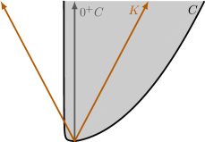
(a) The approximate recession cone $K$ as computed in lines 1-5.

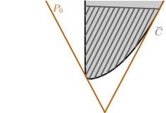
(b) $P_{0}$ is the initial approximation of $C$ according to (16). The grey hatched area is the compact subset $\mskip 1.5mu\overline{\mskip-1.5mu{C}\mskip-1.5mu}\mskip 1.5mu$ of $C$ computed in line 6.

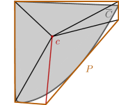
(c) One iteration of Algorithm 1 applied to $\mskip 1.5mu\overline{\mskip-1.5mu{C}\mskip-1.5mu}\mskip 1.5mu$ in line 7. The line segments connecting vertices of the current approximation $P$ with the interior point $c$ correspond to the directions for which the subproblems (P₂($v,d$)) are solved. The vertex from which the red line segment is emanating yields the largest distance to $\mskip 1.5mu\overline{\mskip-1.5mu{C}\mskip-1.5mu}\mskip 1.5mu$.

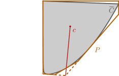
(d) The updated approximation after a vertex of the approximation in Figure 3(c) is cut off. The red line segment and the new facet of $P$ intersect the boundary of $\mskip 1.5mu\overline{\mskip-1.5mu{C}\mskip-1.5mu}\mskip 1.5mu$ in the same point.

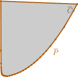
(e) $\mskip 1.5mu\overline{\mskip-1.5mu{P}\mskip-1.5mu}\mskip 1.5mu$ is the computed $\varepsilon$-approximation of $\mskip 1.5mu\overline{\mskip-1.5mu{C}\mskip-1.5mu}\mskip 1.5mu$ after Algorithm 1 terminates in line 7. The orange dots are the vertices of $\mskip 1.5mu\overline{\mskip-1.5mu{C}\mskip-1.5mu}\mskip 1.5mu$.

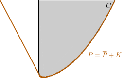
(f) The $\left(\varepsilon,\delta\right)$-approximation $P$ of $C$ that is computed by the algorithm.

 

Figure 3: The computed polyhedra at different steps of Algorithm 2 for the error tolerances $\left(\varepsilon,\delta\right)=(0.1,0.1)$. Figures 3(a) and 3(c)-3(f) are scaled vertically by a factor of 0.077, Figure 3(b) by a factor of 0.054 for visibility.

Table 1: Computational results for Example 5.1 and different values of $\varepsilon$ and $\delta$. Every cell shows the number of solved semidefinite subproblems, the number of vertices of the polyhedral approximation, as well as the elapsed CPU time.

	0.1	0.15	0.2
0.1	603 26 230.98	359 20 139.92	261 16 100.22
0.3	239 15 93.57	161 12 62.79	99 9 39.15
0.5	198 14 76.38	99 9 38.76	99 9 39.85

Computational results for different values of $\varepsilon$ and $\delta$ are presented in Table 1. It can be seen that the number of subproblems that have to be solved is larger than the number of vertices the polyhedral approximation has. The reason is that one instance of (P₂($v,d$)) is solved for every vertex of the current approximation in every iteration of Algorithm 1, but only one of these vertices is cut off. Moreover, the number of solved subproblems grows quickly as $\varepsilon$ decreases, because more iterations of Algorithm 1 are needed to reach the desired accuracy and the number of solved subproblems grows with every iteration. Since the recession cone of $C$ is just a ray and easy to approximate, most of the computational effort is put into approximating $\mskip 1.5mu\overline{\mskip-1.5mu{C}\mskip-1.5mu}\mskip 1.5mu$ in line 7. However, for fixed $\varepsilon$ and decreasing $\delta$ the number of solved subproblems grows. This is due to the fact that $\mskip 1.5mu\overline{\mskip-1.5mu{C}\mskip-1.5mu}\mskip 1.5mu$ depends on the approximate recession cone $K$. As $\delta$ decreases the rays generating $K$ will be closer to each other with respect to the truncated Hausdorff distance. Therefore, the set $\mskip 1.5mu\overline{\mskip-1.5mu{C}\mskip-1.5mu}\mskip 1.5mu$ will have a larger area and it takes more iterations to compute an $\varepsilon$-approximation of it. Note, that for $\left(\varepsilon,\delta\right)$ equal to $(0.3,0.2)$, $(0.5,0.15)$ or $(0.5,0.2)$ the same number of subproblems are solved and the approximations have the same number of vertices. For the tolerances $(0.3,0.2)$ and $(0.5,0.2)$ the values are identical, because during the approximation of $\mskip 1.5mu\overline{\mskip-1.5mu{C}\mskip-1.5mu}\mskip 1.5mu$ the approximation error in Algorithm 1 changes from a value larger than 0.5 to a value smaller than 0.3 in one iteration. Therefore, the resulting $\left(\varepsilon,\delta\right)$-approximations are identical. For $\left(\varepsilon,\delta\right)=(0.5,0.15)$ the approximation is different and it is a coincidence that the values coincide.

Example 5.2.

Algorithm 2 can also be used to compute polyhedral approximations of closed and pointed convex cones. Consider for example the positive semidefinite cone of $2\times 2$ matrices

$$S=\left\{x\in\mathbb{R}^{3}\middle|\begin{pmatrix}x_{1}&x_{3}\\ x_{3}&x_{2}\end{pmatrix}\succcurlyeq 0\right\}.$$

It is a closed and pointed convex cone with nonempty interior. Thus, we can apply Algorithm 2 to it. Since $S$ is a cone, its only vertex is the origin and we can terminate the algorithm after $K$ has been computed in line 5. Then $K$ is a polyhedral cone and it holds $\bar{d}_{\mathsf{H}}(K,S)\leq\delta$. Figure 4 shows a polyhedral approximation of $S$ with 20 extreme rays and $\bar{d}_{\mathsf{H}}(K,S)\leq 0.1$.

 

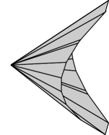
Figure 4: A polyhedral approximation of the cone of $2\times 2$ positive semidefinite matrices obtained by Algorithm 2 for $\delta=0.1$, see Example 5.2.

6 Conclusion

We have introduced the notion of $\left(\varepsilon,\delta\right)$-approximations for the polyhedral approximation of unbounded convex sets. Since polyhedral approximation in the Hausdorff distance can only be achieved for unbounded sets under restrictive assumptions, $\left(\varepsilon,\delta\right)$-approximations are of particular interest, because they allow treatment of a larger class of sets. An important observation is that the recession cones of the involved sets must play a crucial role in a meaningful concept of approximation for unbounded sets. We have shown that $\left(\varepsilon,\delta\right)$-approximations define a suitable notion of approximation in the sense that a sequence of such approximations convergences and that $\left(\varepsilon,\delta\right)$-approximations generalize the polyhedral approximation of compact sets with respect to the Hausdorff distance. Finally, we have presented an algorithm that allows for the computation of $\left(\varepsilon,\delta\right)$-approximations of spectrahedra and have shown that the algorithm is finite.

Data Availability Statement

Data sharing is not applicable to this article as no datasets were generated or analysed during the current study.

References

- Boyd and Vandenberghe [2004] S. Boyd and L. Vandenberghe. Convex Optimization. Cambridge University Press, Cambridge, 2004.
- Bronshteĭn [2007] E. M. Bronshteĭn. Approximation of convex sets by polyhedra. Sovrem. Mat. Fundam. Napravl. 22 (2007), pp. 5–37.
- Bronshteĭn and Ivanov [1975] E. M. Bronshteĭn and L. D. Ivanov. The approximation of convex sets by polyhedra. Sibirsk. Mat. Ž. 16 (1975), pp. 1110–1112, 1132.
- Cheney and Goldstein [1959] E. W. Cheney and A. A. Goldstein. Newton’s method for convex programming and Tchebycheff approximation. Numer. Math. 1 (1959), pp. 254–268.
- Ciripoi [2019] D. Ciripoi. Approximation of Spectrahedral Shadows and Spectrahedral Calculus. Ph.D. thesis, Friedrich Schiller University Jena, 2019.
- Ciripoi et al. [2018] D. Ciripoi, A. Löhne, and B. Weißing. A vector linear programming approach for certain global optimization problems. J. Global Optim. 72 (2018), pp. 347–372.
- Duran and Grossmann [1986] M. A. Duran and I. E. Grossmann. An outer-approximation algorithm for a class of mixed-integer nonlinear programs. Math. Programming 36 (1986), pp. 307–339.
- Dörfler et al. [2021] D. Dörfler, A. Löhne, C. Schneider, and B. Weißing. A benson-type algorithm for bounded convex vector optimization problems with vertex selection. Optimization Methods and Software 0 (2021), pp. 1–21.
- Eaton et al. [2021] J. W. Eaton, D. Bateman, S. Hauberg, and R. Wehbring. GNU Octave version 6.3.0 manual: a high-level interactive language for numerical computations, 2021. URL https://www.gnu.org/software/octave/doc/v6.3.0/.
- Ehrgott et al. [2011] M. Ehrgott, L. Shao, and A. Schöbel. An approximation algorithm for convex multi-objective programming problems. J. Global Optim. 50 (2011), pp. 397–416.
- Fejes Tóth [1948] L. Fejes Tóth. Approximation by polygons and polyhedra. Bull. Amer. Math. Soc. 54 (1948), pp. 431–438.
- Goberna et al. [2013] M. A. Goberna, A. Iusem, J. E. Martínez-Legaz, and M. I. Todorov. Motzkin decomposition of closed convex sets via truncation. J. Math. Anal. Appl. 400 (2013), pp. 35–47.
- Goldman and Ramana [1995] A. J. Goldman and M. Ramana. Some geometric results in semidefinite programming. J. Global Optim. 7 (1995), pp. 33–50.
- Gurariĭ [1965] V. I. Gurariĭ. Openings and inclinations of subspaces of a Banach space. Teor. Funkciĭ Funkcional. Anal. i Priložen. Vyp. 1 (1965), pp. 194–204.
- Holmes [1975] R. B. Holmes. Geometric Functional Analysis and its Applications. Springer-Verlag, New York-Heidelberg, 1975. Graduate Texts in Mathematics, No. 24.
- Iusem and Seeger [2010] A. Iusem and A. Seeger. Distances between closed convex cones: old and new results. J. Convex Anal. 17 (2010), pp. 1033–1055.
- Kamenev [1992] G. K. Kamenev. A class of adaptive algorithms for the approximation of convex bodies by polyhedra. Zh. Vychisl. Mat. i Mat. Fiz. 32 (1992), pp. 136–152.
- Kamenev [1993] G. K. Kamenev. Efficiency of Hausdorff algorithms for polyhedral approximation of convex bodies. Zh. Vychisl. Mat. i Mat. Fiz. 33 (1993), pp. 796–805.
- Kamenev [1994] G. K. Kamenev. Analysis of an algorithm for approximating convex bodies. Zh. Vychisl. Mat. i Mat. Fiz. 34 (1994), pp. 608–616.
- Kelley [1960] J. E. Kelley, Jr. The cutting-plane method for solving convex programs. J. Soc. Indust. Appl. Math. 8 (1960), pp. 703–712.
- Khachiyan et al. [2008] L. Khachiyan, E. Boros, K. Borys, K. Elbassioni, and V. Gurvich. Generating all vertices of a polyhedron is hard. Discrete Comput. Geom. 39 (2008), pp. 174–190.
- Kronqvist et al. [2016] J. Kronqvist, A. Lundell, and T. Westerlund. The extended supporting hyperplane algorithm for convex mixed-integer nonlinear programming. J. Global Optim. 64 (2016), pp. 249–272.
- Löhne [2011] A. Löhne. Vector Optimization with Infimum and Supremum. Vector optimization. Springer, Heidelberg, 2011.
- Löhne et al. [2014] A. Löhne, B. Rudloff, and F. Ulus. Primal and dual approximation algorithms for convex vector optimization problems. J. Global Optim. 60 (2014), pp. 713–736.
- Löhne and Weißing [2016] A. Löhne and B. Weißing. Equivalence between polyhedral projection, multiple objective linear programming and vector linear programming. Math. Methods Oper. Res. 84 (2016), pp. 411–426.
- Lubin et al. [2018] M. Lubin, E. Yamangil, R. Bent, and J. P. Vielma. Polyhedral approximation in mixed-integer convex optimization. Math. Program. 172 (2018), pp. 139–168.
- Minkowski [1903] H. Minkowski. Volumen und Oberfläche. Math. Ann. 57 (1903), pp. 447–495.
- Netzer [2011] T. Netzer. Spectrahedra and their Shadows. Habilitation thesis, University of Leipzig, 2011.
- Ney and Robinson [1995] P. E. Ney and S. M. Robinson. Polyhedral approximation of convex sets with an application to large deviation probability theory. J. Convex Anal. 2 (1995), pp. 229–240.
- Rockafellar [1997] R. T. Rockafellar. Convex Analysis. Princeton Landmarks in Mathematics. Princeton University Press, Princeton, NJ, 1997. Reprint of the 1970 original, Princeton Paperbacks.
- Rockafellar and Wets [1998] R. T. Rockafellar and R. J.-B. Wets. Variational Analysis, vol. 317 of Grundlehren der Mathematischen Wissenschaften [Fundamental Principles of Mathematical Sciences]. Springer-Verlag, Berlin, 1998.
- Ruzika and Wiecek [2005] S. Ruzika and M. M. Wiecek. Approximation methods in multiobjective programming. J. Optim. Theory Appl. 126 (2005), pp. 473–501.
- Schneider [1981] R. Schneider. Zur optimalen Approximation konvexer Hyperflächen durch Polyeder. Math. Ann. 256 (1981), pp. 289–301.
- Toh et al. [1999] K. C. Toh, M. J. Todd, and R. H. Tütüncü. SDPT3—a MATLAB software package for semidefinite programming, version 1.3. Optim. Methods Softw. 11/12 (1999), pp. 545–581.
- Tütüncü et al. [2003] R. H. Tütüncü, K. C. Toh, and M. J. Todd. Solving semidefinite-quadratic-linear programs using SDPT3. Math. Program. 95 (2003), pp. 189–217.
- Ulus [2018] F. Ulus. Tractability of convex vector optimization problems in the sense of polyhedral approximations. J. Global Optim. 72 (2018), pp. 731–742.
- Varadhan [1984] S. R. S. Varadhan. Large deviations and applications, vol. 46 of CBMS-NSF Regional Conference Series in Applied Mathematics. Society for Industrial and Applied Mathematics (SIAM), Philadelphia, PA, 1984.
- Veinott [1967] A. F. Veinott, Jr. The supporting hyperplane method for unimodal programming. Operations Res. 15 (1967), pp. 147–152.
- Westerlund and Pettersson [1995] T. Westerlund and F. Pettersson. An extended cutting plane method for solving convex minlp problems. Computers & Chemical Engineering 19 (1995), pp. 131–136.