Estimating Entropy Production Rates with First-Passage Processes

Abstract

We consider the problem of estimating the mean entropy production rate in a nonequilibrium process from the measurements of first-passage quantities associated with a single current. For first-passage processes with large thresholds, Refs. [1, 2] identified a ratio of first-passage observables — involving the mean first-passage time, the splitting probability, and the first-passage thresholds— that lower bounds the entropy production rate and is an unbiased estimator of the entropy production rate when applied to a current that is proportional to the stochastic entropy production. Here, we show that also at finite thresholds, a finite number of realisations of the nonequilibrium process, and for currents that are not proportional to the stochastic entropy production, first-passage ratios can accurately estimate the rate of dissipation. In particular, first-passage ratios capture a finite fraction of the total entropy production rate in regimes far from thermal equilibrium where thermodynamic uncertainty ratios capture a negligible fraction of the total entropy production rate. Moreover, we show that first-passage ratios incorporate nonMarkovian statistics in the estimated value of the dissipation rate, which are difficult to include in estimates based on Kullback-Leibler divergences. Taken together, we show that entropy production estimation with first-passage ratios is complementary to estimation methods based on thermodynamic uncertainty ratios and Kullback-Leibler divergences.

1 Introduction

Empirical measurements of dissipated heat in nonequilibrium, mesoscopic systems are challenging. The obstacle is that heat, defined as the remainder energy required to satisfy the first law of thermodynamics [3], is microscopically the energy exchanged between a system and its environment through interactions with a large number of microscopic degrees of freedom [4]. Therefore, contrarily to the work performed on a system, heat cannot be measured directly.

To illustrate the empirical difficulty of measuring heat in small systems, let us consider the example of a molecular motor in a living cell. A molecular motor dissipates at a power of $10^{-18}W$ [5, 6, 7], which is several orders of magnitude smaller than the $10^{-6}W$ sensitivity of calorimeters [8, 9]. Nevertheless, even if it were possible to measure heat at an accuracy of $10^{-18}W$, then still it would not be possible to measure the rate of dissipation of a molecular motor in a living cell, as in living cells a large number of dissipative processes take place at once. Therefore, it is important to develop alternative methods to measure dissipation in nonequilibrium, mesoscopic systems.

Instead of measuring the rate $\dot{s}$ of dissipation, also known as the entropy production rate, with calorimeters, the entropy production rate can be estimated from the trajectories of slow, coarse-grained degrees of freedom, which is an example of a thermodynamic inference problem [10]. In this paper, we consider entropy production estimation based on the trajectories of a single current $J$ in a stationary process. An observer measures, e.g., the current in an electrical wire or the position of a molecular motor bound to a biofilament, and aims to estimate the rate of dissipation from the obtained trajectories. If the average current $\langle J(t)\rangle\neq 0$, then the system is driven out of equilibrium. However, in general, it is not possible to estimate the rate of dissipation from the average current, except when the thermodynamic affinity is known. On the other hand, when the whole trajectory of the current $J$ is available, then it is possible to estimate the entropy production rate from fluctuations in the current [11].

An estimator of dissipation is a real-valued functional evaluated on the trajectories of a nonequilibrium process. In the present paper we limit ourselves to estimators that are evaluated on the trajectories of a single current $J$, and we also consider estimators that do not require knowledge about the model that determines the statistics of the nonequilibrium process $X$. These two limitations model physical scenarios for which only partial information about the nonequilibrium process is available, such as, the case when the position of a molecular motor is measured, but the chemical states of its motor heads are not known.

The quality of an estimator is determined by its bias, i.e., the distance between the average value of the estimator and the rate of dissipation. Since we consider problems with partial information, it is in general not possible to obtain an unbiased estimator. In fact, when observing a single current, a good estimator of dissipation will underestimate the amount of dissipation in the process, as in general there exist other dissipative processes that do not directly influence the measured current. A notable exception is when the current $J$ is proportional to the stochastic entropy production. In this case, we expect a good estimator to be unbiased. Lastly, let us mention that the bias of an estimator can depend on the number of trajectories available. In other words, an estimator may have a small bias in the limit of an infinite number of realisations of a nonequilibrium process, while in situations of finite data the same estimator may have a large bias.

As the entropy production estimation problem has been considered before, we first review two estimators that have been well studied in the literature. Subsequently, we present an estimator based on first-passage processes that has been less studied, and which constitutes the main topic of this paper.

The first estimator that we review is the Kullback-Leibler divergence between the probability to observe a trajectory of a current and the probability to observe its time-reversed trajectory, see e.g., Refs. [12, 13, 14, 15, 16, 17]. In general, it is however impractical to evaluate the Kullback-Leibler divergence. This because the statistics of a single current $J$ are nonMarkovian, which complicates significantly the evaluation of the probability to observe a certain trajectory. Because of this complication, nonMarkovian effects in the current are often neglected by evaluating [12, 13, 14]

$$\hat{s}_{\rm KL}:=\sum_{j\in\mathcal{J}}\dot{n}_{j}\log\frac{\dot{n}_{j}}{\dot{n}_{-j}},$$ (1)

where $\dot{n}_{j}$ is the rate at which the current $J$ makes a jump of size $j$, and $\mathcal{J}$ is the set of possible jump sizes. The estimator (1) neglects nonMarkovian statistics in $J$’s trajectory, and consequently the estimator is biased, i.e., $\hat{s}_{\rm KL}\leq\dot{s}$.

A second estimator of dissipation that we review is the Thermodynamic Uncertainty Ratio (TUR) [18, 11, 10, 19, 20]

$$\hat{s}_{\rm TUR}:=\frac{2\overline{j}^{2}t}{\sigma^{2}_{J(t)}},$$ (2)

where $J(t)$ is a stochastic current at time $t$, $\overline{j}=\langle J(t)\rangle/t$ is the average current rate, and $\sigma^{2}_{J(t)}=\langle J^{2}(t)\rangle-\langle J(t)\rangle^{2}$ is the variance of the current. The TUR has been proposed as an estimator of dissipation as it lower bounds the entropy production rate in stationary Markov jump processes and overdamped Langevin processes, i.e., $\hat{s}_{\rm TUR}\leq\dot{s}$. However, the bias of the TUR is large for systems far from thermal equilibrium. For example, it was shown that $\hat{s}_{\rm TUR}$ captures 20 % of the total dissipation of molecular motors, such as kinesin and myosin [6, 7], and the bias of the TUR remains large when $J$ equals the stochastic entropy production [21].

In an attempt of resolving the issues in the bias of the Kullback-Leibler divergence and the TUR, we study in this paper the First-Passage Ratio (FPR) [1, 2]

$$\hat{s}_{\rm FPR}(\ell_{+},\ell_{-}):=\left\{\begin{array}[]{ccc}\frac{\ell_{+}}{\ell_{-}}\frac{1}{\langle T_{J}\rangle}\left|\ln p_{-}\right|,&&\overline{j}>0,\\ \frac{\ell_{-}}{\ell_{+}}\frac{1}{\langle T_{J}\rangle}\left|\ln p_{+}\right|,&&\overline{j}<0,\end{array}\right.$$ (3)

where $T_{J}$ is the first time when the stochastic current $J$ leaves the open interval $(-\ell_{-},\ell_{+})$ with $\ell_{-},\ell_{+}>0$, $p_{-}$ is the probability that $J$ first goes below the negative threshold $-\ell_{-}$ before exceeding the positive value $\ell_{+}$, and $p_{+}=1-p_{-}$. For stationary Markov jump processes and in the limit of large thresholds $\ell_{-}$ and $\ell_{+}$, the FPR bounds the dissipation rate from below, i.e., $\hat{s}_{\rm FPR}\leq\dot{s}$[1, 2]. In addition, the FPR is an unbiased estimator when $J$ is proportional to the stochastic entropy production [1, 2], i.e., $\hat{s}_{\rm FPR}=\dot{s}$, a result that also holds in the limit of large thresholds.

Although it was established that $\hat{s}_{\rm FPR}$ equals $\dot{s}$ for large thresholds and for currents that are proportional to the stochastic entropy production, this is not sufficient to conclude that $\hat{s}_{\rm FPR}$ is a useful estimator of dissipation. Therefore, in the present paper, we determine the bias in the estimator $\hat{s}_{\rm FPR}$ for: (i) generic currents that are not proportional to the entropy production; (ii) finite thresholds $\ell_{+}$ and $\ell_{-}$; and (iii) a finite number of realisations of the nonequilibrium process. To this aim, we estimate dissipation based on the FPR in two paradigmatic examples of nonequilibrium Markov jump processes, namely, a random walker on a two-dimensional lattice [see Fig. 1(a)] and a model for a molecular motor with two motor heads [see Fig. 1(b)]. To evaluate the quality of $\hat{s}_{\rm FPR}$, we compare the bias in the estimates of dissipation based on the FPR with those based on the TUR and the Kullback-Leibler divergence.

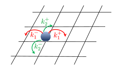
(a) Random walk on a two-dimensional lattice

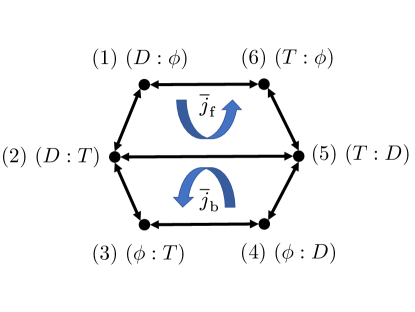
(b) Six state model for molecular motors with two motor heads, such as, conventional kinesin

Figure 1: Illustration of the two paradigmatic examples of nonequilibrium processes that we consider in this paper. Subfigure (a): Random walker jumping on a two-dimensional lattice at rates $k^{+}_{1}$, $k^{-}_{1}$, $k^{+}_{2}$, and $k^{-}_{2}$. Subfigure (b): Markov jump process with six states, representing the different chemical configurations of the two motor heads of a molecular motor bound to a biofilament [22, 6]. The different motor states are ATP bound (T), ADP bound (D), and nucleotide free ($\phi$). Since there are six states, we also label them with $\left\{1,2,3,4,5,6\right\}$ as indicated in the figure. The motor moves forwards along the cycle ($2\rightarrow 5\rightarrow 6\rightarrow 1\rightarrow 2$) and moves backwards along the cycle ($5\rightarrow 2\rightarrow 3\rightarrow 4\rightarrow 5$) at rates $\overline{j}_{\rm f}$ and $\overline{j}_{\rm b}$, respectively.

The paper is organised as follows: In Sec. 2, we introduce the setup of stationary Markov jump processes that we use in this paper, and we define entropy production in this setup. In Sec. 3, we define estimators of entropy production based on the FPR, the TUR, and the Kullback-Leibler divergence. In Sec. 4, we make a study of $\hat{s}_{\rm FPR}$ as an estimator of the entropy production rate in a two-dimensional random walk process, and in Sec. 5, we make an analogous study for a model of a molecular motor with two motor heads, such as, conventional kinesin. We end the paper with a discussion in Sec. 6, where we compare the advantages and disadvantages of the different estimators for dissipation. The paper also contains three appendices with detailed information on some of the calculations and the parameters used in the models.

2 Entropy production in stationary Markov jump processes

We first present in Sec. 2.1 the mathematical setup on which we work in this paper, and in Sec. 2.2 we discuss the physical context of the mathematical setup.

2.1 General system setup

We focus in this paper on stationary Markov jump processes [23], which play an important role in stochastic thermodynamics [24, 25]; doing so, we neglect the possibility of a Hamiltonian evolution [26].

Let $X(t)$ be a Markov jump process taking values in a discrete set $\mathcal{X}$ [23], with $t\geq 0$ a time index. We denote by $\mathbb{P}$ the probability measure that generates the statistics of $X$, and averages with respect to $\mathbb{P}$ are denoted by $\langle\cdot\rangle_{\mathbb{P}}$, or more briefly $\langle\cdot\rangle$. Trajectories of $X(t)$ are denoted by $X^{t}_{0}$.

We assume that the process $X$ is regular, i.e., it has a finite number of jumps within each time interval of finite length. The probability distribution $p_{X(t)}(x)=p(x;t)$ of $X(t)$ solves Kolmogorov’s backward differential system [23]

$$\partial_{t}p(x;t)=\sum_{y\in\mathcal{X}\setminus x}p(y;t)w_{y\rightarrow x}-p(x;t)\sum_{y\in\mathcal{X}\setminus x}w_{x\rightarrow y},\quad{\rm for}\quad x\in\mathcal{X},$$ (4)

where $w_{x\rightarrow y}\in\mathbb{R}^{+}$ are the transition rates to jump from $x$ to $y$. We consider time-homogeneous Markov jump processes for which the rates $w_{y\rightarrow x}$ are independent of time $t$.

We assume that $X$ admits a unique stationary probability distribution $p_{\rm ss}(x)$ with $p_{\rm ss}(x)>0$ for all $x\in\mathcal{X}$, and we set $p_{X(0)}(x)=p_{\rm ss}(x)$, so that the process is stationary. As shown in Ref. [23], in this setup it holds that for generic initial conditions the stationary state is reached in a finite time, i.e., $\lim_{t\rightarrow\infty}p(x;t)=p_{\rm ss}(x)$, and moreover the ergodic theorem implies that $\lim_{t\rightarrow\infty}t^{-1}\int^{t}_{0}f(X(s)){\rm d}s=\sum_{x\in\mathcal{X}}f(x)p_{\rm ss}(x)$ for all initial distributions and real-valued functions $f$ with $\sum_{x\in\mathcal{X}}|f(x)|p_{\rm ss}(x)<\infty$ [23]. Note that for finite sets $\mathcal{X}$, a sufficient requirement for the uniqueness of the stationary probability distribution is that the graph of nonzero transitions $w_{x\rightarrow y}$ is strongly connected — a property that is often called irreducibility— and for countable sets $\mathcal{X}$ we also require that the process is $t$-positive recurrent, i.e., the mean time for $X$ to return to its initial state is finite [23].

The last assumption we require is that the Markov jump process is reversible in the sense that

$$w_{x\rightarrow y}=0\Leftrightarrow w_{y\rightarrow x}=0,\quad\forall x,y\in\mathcal{X}.$$ (5)

Given the above assumptions, we can define the stochastic entropy production by [27, 25]

$$S(t):=\frac{1}{2}\sum_{x,y\in\mathcal{X}}J_{x\rightarrow y}(t)\ln\frac{p_{\rm ss}(x)w_{x\rightarrow y}}{p_{\rm ss}(y)w_{y\rightarrow x}},$$ (6)

where the edge currents

$$J_{x\rightarrow y}(t)=N_{x\rightarrow y}(t)-N_{y\rightarrow x}(t)$$ (7)

denote the difference between the number of times $N_{x\rightarrow y}(t)$ the process $X$ has jumped from $x$ to $y$ in the time interval $[0,t]$ and the number of times $N_{y\rightarrow t}(t)$ the process $X$ has jumped from $y$ to $x$ in the same time interval. We denote the mean entropy production rate by

$$\dot{s}:=\langle S(t)\rangle_{\mathbb{P}}/t=\sum_{x,y\in\mathcal{X}}p_{\rm ss}(x)w_{x\rightarrow y}\ln\frac{p_{\rm ss}(x)w_{x\rightarrow y}}{p_{\rm ss}(y)w_{y\rightarrow x}},$$ (8)

which will be the main quantity of interest in this paper.

2.2 Physical interpretation of $\dot{s}$ based on local detailed balance

To give physical content to the entropy production rate $\dot{s}$— in the sense of dissipation or the entropy production of the second law of thermodynamics — it is necessary to make physical assumptions about the nature of the environment and the interactions between the system and its environment. It should be emphasised that these physical assumptions are mathematically superfluous, as they do not alter the model setup given by Eq. (4). Indeed, Eq. (4) provides a coarse-grained description of a system for which environmental degrees of freedom have already been integrated out. Nevertheless, to understand the physical relevance of $\dot{s}$, it is necessary to consider how Eq. (8) appears in the broader picture of a system coupled to an environment.

We assume that $X\in\mathcal{X}$ represents the slow, coarse-grained degrees of freedom of a mesoscopic system that is in contact with one or more equilibrium reservoirs. A given mesoscopic configuration $x\in\mathcal{X}$ has an energy $u(x)$ and an entropy $s_{\rm int}(x)$ due to the existence of fast, internal degrees of freedom.

Following Refs. [28, 24, 29, 25], we use the principle of local detailed balance, which states that

$$\frac{w_{x\rightarrow y}}{w_{y\rightarrow x}}=e^{s_{xy}},\quad{\rm with}\quad x,y\in\mathcal{X},$$ (9)

where $s_{xy}(=-s_{yx})$ is the change of entropy in the environment and the fast, internal degrees of freedom of the system when $X$ jumps from $x$ to $y$. Note that Eq. (9) does not require that the system is near equilibrium — as $\dot{s}$ can be large — but it does require that the environment is equilibrated. To have a system far from thermal equilibrium that interacts with an environment in equilibrium, we require, in general, weak coupling between system and environment and fast relaxation of the degrees of freedom in the environment.

The precise form of $s_{xy}$ depends on the physical problem of interest. For a system in thermal equilibrium,

$$s_{xy}=\frac{f(x)-f(y)}{\mathsf{T}_{\rm env}},$$ (10)

where $f(x)=u(x)-\mathsf{T}_{\rm env}\>s_{\rm int}(x)$ is the free energy of the $x$-th state, and $\mathsf{T}_{\rm env}$ is the temperature of the environment. Note that we use natural units for which Boltzmann’s constant is set to one. For a nonequilibrium system in contact with a thermal reservoir, Eq. (10) extends to

$$s_{xy}=s_{\rm int}(y)-s_{\rm int}(x)-\frac{Q}{\mathsf{T}_{\rm env}},$$ (11)

where $Q$ is the net heat absorbed by the system from the environment. Equation (11) provides a direct link between the entropy production rate $\dot{s}$, as defined in Eq. (8), and the rate of heat dissipated to the environment,

$$\dot{s}=-\frac{\langle Q(t)\rangle}{t\mathsf{T}_{\rm env}}.$$ (12)

Therefore, in this paper, we call $\dot{s}$ the entropy production rate, as well as, the rate of dissipation.

As a last example, let us consider the case of a molecular motor that interacts with $m$ chemostats at chemical potentials $\mu_{\alpha}$, with $\alpha=1,2,\ldots,m$, and an external agent that exerts a mechanical force $f_{\rm mech}$ on the motor. In this example [18]

$$s_{xy}=\frac{f(x)-f(y)}{\mathsf{T}_{\rm env}}+\sum^{m}_{\alpha=1}\frac{\mu_{\alpha}}{\mathsf{T}_{\rm env}}n_{\alpha}(x,y)-\frac{f_{\rm mech}\delta(x,y)}{\mathsf{T}_{\rm env}},$$ (13)

where $n_{\alpha}(x,y)$ is the number of particles exchanged with the $\alpha$-th reservoir when $X$ jumps for $x$ to $y$, and $\delta(x,y)$ is the distance moved by the motor when $X$ jumps for $x$ to $y$. We follow the usual convention that $n_{\alpha}>0$ when the system binds particles and $n_{\alpha}<0$ when the system releases particles [3]. The minus sign in front of $f_{\rm mech}$ implies that the mechanical force opposes the motion of the motor when it moves forward.

3 Estimators of $\dot{s}$ that rely on the measurement of a single current

We aim to infer $\dot{s}$ based on the measurements of a single stochastic current of the form

$$J(t):=\sum_{x,y\in\mathcal{X}}c_{x,y}J_{x\rightarrow y}(t),$$ (14)

where $c_{x,y}\in\mathbb{R}$; observe that the stochastic entropy production $S$, as defined in (6), is a specific example of a current. If $J=cS$, with $c$ a constant, then this is equivalent to an estimation problem with complete information, while otherwise, this is an estimation problem with partial information. Without loss of generality, we assume in what follows that $\langle J(t)\rangle/t=\overline{j}>0$.

3.1 Estimators of dissipation: general definitions

Given $n_{s}$ independent realisations $J^{(i)}(t)$ of a current $J(t)$, with $i=1,2,\ldots,n_{\rm s}$, an estimator $\mathcal{F}(\vec{J}^{t}_{0})$ of $\dot{s}$ is a functional defined on the set of trajectories $\vec{J}^{t}_{0}=([J^{(1)}]^{t}_{0},[J^{(2)}]^{t}_{0},\ldots,[J^{(n_{\rm s})}]^{t}_{0})$.

The bias of the estimator $\mathcal{F}$ is its average value

$$\langle\mathcal{F}(\vec{J}^{t}_{0})\rangle=\hat{s}+g(n_{\rm s}),$$ (15)

where

$$\hat{s}=\lim_{n_{\rm s}\rightarrow\infty}\langle\mathcal{F}(\vec{J}^{t}_{0})\rangle$$ (16)

is the bias of the estimator in the asymptotic limit of an infinite number of realisations, and $g(n_{\rm s})$ is a function that determines how the bias depends on $n_{\rm s}$; note that $g(n_{\rm s})\rightarrow 0$ for $n_{\rm s}\gg 1$. An estimator is unbiased in the limit of an infinite number of realisations when $\hat{s}=\dot{s}$, and it is an unbiased estimator, tout court, when both $\hat{s}=\dot{s}$ and $g=0$.

In what follows, we define three estimators of $\dot{s}$, namely, $\mathcal{F}_{\rm FPR}$ based on the FPR, $\mathcal{F}_{\rm TUR}$ based on the TUR, and $\mathcal{F}_{\rm KL}$ based on the Kullback-Leibler divergence. As we discuss, all the estimators capture a finite fraction of the dissipation, i.e.

$$\hat{s}\leq\dot{s},$$ (17)

but the equality is attained in different circumstances. Consequently, all the functionals we introduce are useful as estimators of dissipation, but they capture dissipation in different scenarios.

3.2 An estimator based on the first-passage ratio $\hat{s}_{\rm FPR}$ (FPR)

3.2.1 Definition.

We define an estimator $\mathcal{F}_{\rm FPR}$ of $\dot{s}$ for which it holds that

$$\lim_{n_{\rm s}\rightarrow\infty}\mathcal{F}_{\rm FPR}=\hat{s}_{\rm FPR},$$ (18)

where $\hat{s}_{\rm FPR}$ is the first-passage ratio Eq. (3), with

$$T_{J}={\rm inf}\left\{t>0:J(t)\notin(-\ell_{-},\ell_{+})\right\}$$ (19)

and

$$p_{-}=\mathbb{P}\left(J(T_{J})\leq-\ell_{-}\right).$$ (20)

Since an estimator $\mathcal{F}$ is defined on $n_{\rm s}$ trajectories of the current $J$, we consider the first-passage times

$$T^{(i)}_{J}={\rm inf}\left\{t>0:J^{(i)}(t)\notin(-\ell_{-},\ell_{+})\right\}\quad{\rm with}\quad i\in\left\{1,2,\ldots,n_{\rm s}\right\},$$ (21)

associated with the different trajectories $[J^{(i)}]^{t}_{0}$ of the current, and the decision variables

$$D^{(i)}=\left\{\begin{array}[]{ccc}1&{\rm if}&J^{(i)}(T^{(i)})\geq\ell_{+},\\ -1&{\rm if}&J^{(i)}(T^{(i)})\leq-\ell_{-},\end{array}\right.$$ (22)

that determine for each trajectory whether the current crosses first the positive threshold ($D^{(i)}=1$) or crosses first the negative threshold ($D^{(i)}=-1$).

Using $T^{(i)}$ and $D^{(i)}$, we define, assuming $\langle J(t)\rangle>0$, the estimator

$$\mathcal{F}_{\rm FPR}:=\frac{\ell_{+}}{\ell_{-}}\frac{1}{\hat{T}_{J}}\left|\ln\hat{p}_{-}\right|,$$ (23)

where

$$\hat{T}_{J}=\frac{1}{n_{\rm s}}\sum^{n_{\rm s}}_{i=1}T^{(i)}_{J}$$ (24)

is the empirical mean of the first-passage time, and

$$\hat{p}_{-}=\frac{1}{n_{\rm s}}{\rm max}\left\{\sum^{n_{\rm s}}_{i=1}\delta_{D^{(i)},-1},1\right\}$$ (25)

is the empirical estimate of the splitting probability $p_{-}$. Analogously, we can define the estimator $\mathcal{F}_{\rm FPR}$ for $\langle J(t)\rangle<0$.

3.2.2 Bias.

For stationary Markov jump processes, it holds that [1, 2]

$$\frac{\hat{s}_{\rm FPR}}{\dot{s}}\leq 1+o_{\ell_{\rm min}}(1),$$ (26)

where we added $o_{\ell_{\rm min}}(1)$ to indicate that the inequality holds asymptotically for large thresholds $\ell_{\rm min}={\rm min}\left\{\ell_{+},\ell_{-}\right\}$; here $o_{\ell_{\rm min}}(1)$ represents the small-o notation, i.e., a function that converges to zero for large values of $\ell_{\rm min}$.

The equality in Eq. (26) is attained when $J=cS$, with $c$ a constant [1, 2], while for currents that are not proportional to $S$ the estimate is in general biased.

Now, let us discuss how the bias depends on the number of realisations in the process. For small values of $n_{\rm s}$ it holds that

$$\hat{p}_{-}\approx\frac{1}{n_{\rm s}},$$ (27)

as the number of events with $D^{(i)}=-1$ is negligible. Consequently, for $n_{\rm s}\ll 1/p_{-}$, $\langle\mathcal{F}_{\rm FPR}\rangle$ grows logarithmically in $n_{\rm s}$, i.e.,

$$\Big{\langle}\mathcal{F}_{\rm FPR}\Big{\rangle}\approx\frac{\ell_{+}}{\ell_{-}}\frac{1}{\langle T_{J}\rangle}\ln n_{\rm s}\leq\hat{s}_{\rm FPR}.$$ (28)

Notice that in Eq. (28), for our convenience, we have assumed $\langle 1/\hat{T}_{J}\rangle\approx 1/\langle T_{J}\rangle$, as this will not effect the scaling arguments in $n_{\rm s}$. At larger values $n_{\rm s}\gg 1/p_{-}$, the mean value $\langle\mathcal{F}_{\rm FPR}\rangle$ saturates to

$$\langle\mathcal{F}_{\rm FPR}\rangle\approx\hat{s}_{\rm FPR}.$$ (29)

Combining Eq. (28) with Eq. (3), and considering that we assumed $\overline{j}>0$, we obtain

$$\langle\mathcal{F}_{\rm FPR}\rangle=\left\{\begin{array}[]{ccc}\frac{\ell_{+}}{\ell_{-}}\frac{1}{\langle T_{J}\rangle}\ln n_{\rm s}&{\rm if}&n_{\rm s}\ll 1/p_{-},\\ \frac{\ell_{+}}{\ell_{-}}\frac{1}{\langle T_{J}\rangle}|\ln p_{-}|&{\rm if}&n_{\rm s}\gg 1/p_{-}.\end{array}\right.$$ (30)

Equation (30) implies that around $n_{\rm s}\approx 1/p_{-}$ the bias of the estimator saturates to its asymptotic value, and the bias grows logarithmically at smaller values smaller of $n_{\rm s}$.

For the case when $J=S$, martingale theory for $e^{-S}$ provides exact expressions for $p_{-}$ in terms of the thresholds $\ell_{-}$ and $\ell_{+}$ [30, 31, 32]. As shown in A, for Markov jump processes near equilibrium ($\dot{s}\approx 0$),

$$p_{-}=\frac{1-e^{-\ell_{+}}}{e^{\ell_{-}}-e^{-\ell_{+}}},$$ (31)

so that we require a number

$$n_{\rm s}\gg\frac{e^{\ell_{-}}-e^{-\ell_{+}}}{1-e^{-\ell_{+}}}\sim e^{\ell_{-}}$$ (32)

of samples, which grows exponentially in the depth of the negative threshold $\ell_{-}$. For process that are governed far from thermal equilibrium, we obtain instead (see A)

$$p_{-}\leq\frac{1}{e^{{\rm max}\left\{\ell_{-},\Delta s\right\}}-e^{-\ell_{+}}}$$ (33)

where

$$\Delta s={\rm inf}|S(t)-\lim_{\epsilon\rightarrow 0^{+}}S(t-\epsilon)|$$ (34)

is the infimum of the jumps sizes in $S(t)$. Equation (33) implies that the number of samples required grows as

$$n_{\rm s}\gg e^{{\rm max}\left\{\ell_{-},\Delta s\right\}}-e^{-\ell_{+}}\sim e^{{\rm max}\left\{\ell_{-},\Delta s\right\}},$$ (35)

which is exponential in either the depth of the negative threshold $\ell_{-}$ or the minimal jump size $\Delta s$, depending on which one is larger. Hence, for processes that are governed far from thermal equilibrium, the number of samples required is independent of the thresholds, but instead depends on the jumps size $\Delta s$.

3.3 An estimator based on the thermodynamic uncertainty ratio $\hat{s}_{\rm TUR}$ (TUR)

3.3.1 Definition.

We define an estimator $\mathcal{F}_{\rm TUR}$ of $\dot{s}$ for which it holds that

$$\lim_{n_{\rm s}\rightarrow\infty}\mathcal{F}_{\rm TUR}=\hat{s}_{\rm TUR},$$ (36)

where $\hat{s}_{\rm TUR}$ is the thermodynamic uncertainty ratio (2). The corresponding estimator $\mathcal{F}_{\rm TUR}$, defined on a finite number $n_{\rm s}$ of realisations of $X$, is

$$\mathcal{F}_{\rm TUR}:=\frac{2}{t}\frac{\left(\sum^{n_{\rm s}}_{i=1}J^{(i)}(t)\right)^{2}}{n_{\rm s}\sum^{n_{\rm s}}_{i=1}\left(J^{(i)}(t)\right)^{2}-\left(\sum^{n_{\rm s}}_{i=1}J^{(i)}(t)\right)^{2}}.$$ (37)

3.3.2 Bias.

For stationary Markov jump processes, the TUR-relation implies that the bias [33, 34, 35, 36]

$$\frac{\hat{s}_{\rm TUR}}{\dot{s}}\leq 1,$$ (38)

and hence also the TUR captures a finite fraction of the total dissipation.

The equality in Eq. (38) is attained by processes near equilibrium. On the other hand, for processes driven away far from thermal equilibrium, the bias in $\mathcal{F}_{\rm TUR}$ is large, i.e., $\hat{s}_{\rm TUR}\ll\dot{s}$ [21, 37]. Improvements on the TUR exist, but these rely on measurements of both currents and time-integrated empirical measures [38, 39], and thus require more information about the process $X$.

To determine the dependence of $\langle\mathcal{F}_{\rm TUR}\rangle$ on $n_{\rm s}$, we rely on the central limit theorem, from which it follows that

$$\langle\mathcal{F}_{\rm TUR}\rangle=\hat{s}_{\rm TUR}+O\left(\frac{1}{\sqrt{n_{\rm s}}}\right),$$ (39)

where $O$ denotes the big-O notation. The correction term in Eq. (39) is due to sample-to-sample fluctuations in the current.

3.4 An estimator based on the Kullback-Leibler divergence $\hat{s}_{\rm KL}$

3.4.1 Definition.

We define an estimator $\mathcal{F}_{\rm KL}$ of $\dot{s}$ for which it holds that

$$\lim_{n_{\rm s}\rightarrow\infty}\mathcal{F}_{\rm KL}=\dot{s}_{\rm KL},$$ (40)

where $\dot{s}_{\rm KL}$ is defined in Eq. (1).

Consider the set $\mathcal{J}$ of all possible jump sizes $\Delta J(t)=J(t)-\lim_{\epsilon\rightarrow 0^{+}}J(t-\epsilon)$ in $J(t)$, excluding the $\Delta J(t)=0$ case as it does not count as a jump. Let $N^{(i)}_{j}(t)$ denote the number of $\Delta J^{(i)}(t)=j$ occurrences in the trajectory $[J^{(i)}]^{t}_{0}$. Since we assumed that the process is reversible, see Eq. (5), it holds that $-j\in\mathcal{J}$ whenever $j\in\mathcal{J}$. Therefore, we define the estimator

$$\mathcal{F}_{\rm KL}(t):=\sum_{j\in\mathcal{J}}\frac{\sum^{n_{\rm s}}_{i=1}N^{(i)}_{j}(t)}{t\>n_{\rm s}}\ln\frac{\sum^{n_{\rm s}}_{i=1}N^{(i)}_{j}(t)}{{\rm max}\left\{\sum^{n_{\rm s}}_{i=1}N^{(i)}_{-j}(t),1\right\}}$$ (41)

that estimates the entropy production rate assuming that the process is Markovian; $\mathcal{F}_{\rm KL}(t)$ is closely related to the apparent entropy production considered in Refs. [40, 16]. In Eq. (43), it should be understood that $0\log(0)=0$.

3.4.2 Bias.

It holds that [40, 16]

$$\frac{\hat{s}_{\rm KL}}{\dot{s}}\leq 1,$$ (42)

which follows from applying Jensen’s inequality to the definition of $\dot{s}$, which states that $\dot{s}$ is a Kullback-Leibler divegence. The equality is attained when the current $J$ is Markovian and a linear combination of all independent currents in $X$.

We discuss how the bias $\langle\mathcal{F}_{\rm KL}\rangle$ depends on $n_{\rm s}$. Let us assume that $\langle J\rangle>0$, $n_{\rm s}t$ is small, and $\dot{s}$ is large enough, so that $N^{(i)}_{-j}=0$ for $j>0$. In this case,

$$\langle\mathcal{F}_{\rm KL}(t)\rangle\approx\frac{N(t)}{t\>n_{\rm s}}\sum_{j\in\mathcal{J}\cap\mathbb{R}^{+}}w_{j}\ln w_{j}+\frac{N(t)}{t\>n_{\rm s}}\ln N(t).$$ (43)

where

$$N(t)=\sum_{j\in\mathcal{J}}\sum^{n_{\rm s}}_{i=1}N^{(i)}_{j}(t)$$ (44)

is the total number of jumps observed, and

$$w_{j}=\frac{\sum^{n_{\rm s}}_{i=1}N^{(i)}_{j}(t)}{N(t)}$$ (45)

is the fraction of jumps of size $j$. Setting $N(t)/t\approx\dot{n}\>n_{\rm s}$, we obtain that

$$\langle\mathcal{F}_{\rm KL}(t)\rangle\approx\dot{n}\>\sum_{j\in\mathcal{J}\cap\mathbb{R}^{+}}w_{j}\ln w_{j}+\dot{n}\ln\left(\dot{n}\>n_{\rm s}t\right).$$ (46)

Hence, analogous to the FPR, the bias of $\langle\mathcal{F}_{\rm KL}(t)\rangle$ grows logarithmically in the number of samples $n_{\rm s}$ until it reaches its asymptotic value $\hat{s}_{\rm KL}$, and therefore $\langle\mathcal{F}_{\rm KL}(t)\rangle$ takes a form similar to Eq. (30).

In what follows, we compare estimation of dissipation with the three estimators $\mathcal{F}_{\rm FPR}$, $\mathcal{F}_{\rm TUR}$ and $\mathcal{F}_{\rm KL}$, in two paradigmatic examples of nonequilibrium processes. As discussed, this boils down to determining $\hat{s}/\dot{s}$ and $g(n_{\rm s})$, as defined in Eq. (15), for these three estimators.

4 Random walker on a two-dimensional lattice

We use first-passage processes for currents to infer the rate at which a random walker on a two-dimensional lattice produces entropy. In particular, we compare estimates based on $\mathcal{F}_{\rm FPR}$ with those based on $\mathcal{F}_{\rm TUR}$ and $\mathcal{F}_{\rm KL}$.

In Sec. 4.1 we define the model. Subsequently, we analyse in Sec. 4.2 the bias in the estimator $\mathcal{F}_{\rm FPR}$ for currents that are not proportional to $S$, and in Secs. 4.3 and 4.4 we analyse the effect of finite thresholds and a finite number of realisations, respectively, on the bias of $\mathcal{F}_{\rm FPR}$.

4.1 Model definition

We consider a two-dimensional hopping process $X=(X_{1},X_{2})$, with $X_{1},X_{2}\in\left\{1,2,\ldots,n\right\}$ the coordinates of a random walker on a two-dimensional lattice of length $n$ with periodic boundary conditions [see Fig. 1(a) for an illustration]. The coordinates evolve according to

$${\rm d}X_{i}(t)={\rm d}N^{+}_{i}(t)-{\rm d}N^{-}_{i}(t),\quad i\in\left\{1,2\right\},$$ (47)

where $N^{+}_{i}$ and $N^{-}_{i}$ are two counting process with rates $k^{+}_{i}$ and $k^{-}_{i}$, respectively, and the boundary conditions are implemented by setting $X_{i}\pm n=X_{i}$.

We parameterise the rates as

$$k^{+}_{1}=\frac{e^{\nu/2}}{4\cosh(\nu/2)},\quad k^{-}_{1}=\frac{e^{-\nu/2}}{4\cosh(\nu/2)},$$ (48)

and

$$k^{+}_{2}=\frac{e^{\nu\rho/2}}{4\cosh(\nu\rho/2)},\quad k^{-}_{2}=\frac{e^{-\nu\rho/2}}{4\cosh(\nu\rho/2)},$$ (49)

so that the total rate

$$k_{\rm total}=k^{+}_{1}+k^{-}_{1}+k^{+}_{2}+k^{-}_{2}=1.$$ (50)

Notice that the total rate fixes the characteristic time scale of the process. We assume, without loss of generality, that $\nu\geq 0$ and $\rho\geq 1$.

The stochastic entropy production, as defined by (6), is in the present example given by

$$S(t)=\nu X_{1}(t)+\nu\rho X_{2}(t),$$ (51)

as $p_{\rm ss}(x)=1/n^{2}$ independent of $x$. Consequently, the entropy production rate

$$\dot{s}=\nu(k^{+}_{1}-k^{-}_{1})+\nu\rho(k^{+}_{2}-k^{-}_{2}).$$ (52)

From Eqs. (51) and (52) it follows that $\nu$ is the affinity associated with $X_{1}$ and $\rho$ is the ratio between the affinities of $X_{2}$ and $X_{1}$. From a geometric point of view, the stochastic process $S$ in Eq. (51) can be represented as a vector in the $(X_{1},X_{2})$-plane. The parameter $\rho$ fixes the direction of this vector and $\nu$ its magnitude.

Without loss of generality, we can parametrise stochastic currents in this model by

$$J(t)=c(1-\Delta)X_{1}(t)+c(1+\Delta)X_{2}(t).$$ (53)

Since the FPR and TUR are independent of $c$, we set $c=1$. If

$$\Delta=\frac{\rho-1}{\rho+1},$$ (54)

then $J(t)$ is proportional to $S(t)$, which is independent of $\nu$.

In the present model, the currents $J$ are Markovian. This is a peculiar feature of the random walk model as, in general, currents in Markov jump processes are nonMarkovian.

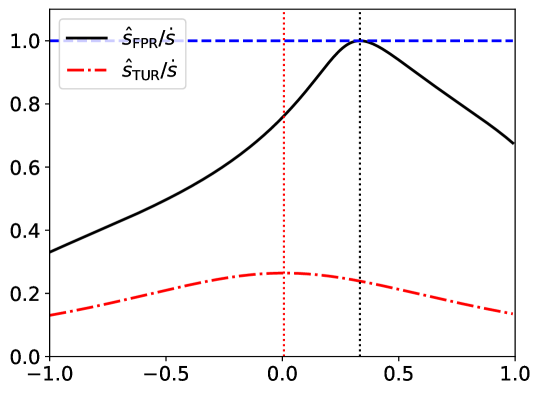
Figure 2: Comparing the bias of FPRs and TURs evaluated on currents in a random walk process on a two-dimensional lattice. The ratios $\hat{s}_{\rm FPR}/\dot{s}$ [in the limit of $\ell_{\rm min}\rightarrow\infty$, given by Eq. (58)] and $\hat{s}_{\rm TUR}/\dot{s}$ [Eq. (60)] are plotted as a function of the parameter $\Delta$ that determines the current $J$. The vertical dotted lines determine the values of $\Delta$ at which $\hat{s}_{\rm FPR}$ and $\hat{s}_{\rm TUR}$ reach their maximum, which are given by $1/3$ [according to Eq. (54)] and $0.0067$ [Eq. (64)], respectively. The rates $k^{+}_{1}$, $k^{-}_{1}$, $k^{+}_{2}$, and $k^{-}_{2}$ are parametrised according to Eqs. (48) and (49), with $\rho=2$ and $\nu=5$; the corresponding value of $\dot{s}\approx 7.5k_{\rm total}$. The ratio $\hat{s}_{\rm TUR}$ is evaluated at $t=20/k_{\rm total}$. The dashed, blue, horizontal line is a guide to the eye that indicates the value $1$ corresponding to optimal thermodynamic inference.

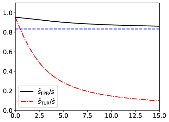
Figure 3: The bias in the FPR and TUR as a function of the rate of dissipation. The ratios $\hat{s}_{\rm FPR}/\dot{s}$ (in the limit of $\ell_{\rm min}\rightarrow\infty$) and $\hat{s}_{\rm TUR}/\dot{s}$ are plotted as a function of the rate of dissipation $\dot{s}/k_{\rm total}$ for the current with $\Delta=0.6$ in the random walk model defined on a two-dimensional lattice. The rates $k^{+}_{1}$, $k^{-}_{1}$, $k^{+}_{2}$, and $k^{-}_{2}$ are parametrised according to Eqs. (48) and (49), with $\rho=2$, while the parameter $\nu$ depends on the rate $\dot{s}$ of dissipation. The horizontal dashed line denotes the asymptotic limit $\lim_{\nu\rightarrow\infty}\hat{s}_{\rm FPR}$ given by Eq. (62).

4.2 Entropy production estimation with currents that are not proportional to $S$

When $J$ is proportional to $S$, then $\hat{s}_{\rm FPR}$ is unbiased in the limit of large thresholds, and hence in this case the FPR is an optimal estimator of dissipation. However, for currents that are not proportional to $S$, $\hat{s}_{\rm FPR}$ is biased. We analyse here the effect of the parameter $\Delta$ that determines the current $J$ on the biases in $\hat{s}_{\rm FPR}$ (in the limit of large thresholds), $\hat{s}_{\rm TUR}$ and $\hat{s}_{\rm KL}$.

In the limit of large thresholds, the mean first-passage time (see Eq. (17) of Ref. [2])

$$\langle T_{J}\rangle=\frac{\ell_{+}}{\overline{j}}=\frac{\ell_{+}}{(1-\Delta)(k^{+}_{1}-k^{-}_{1})+(1+\Delta)(k^{+}_{2}-k^{-}_{2})}$$ (55)

and the splitting probability (see Proposition 7 of Appendix E of [2])

$$p_{-}=e^{\ell_{-}z^{\ast}},$$ (56)

where $z^{\ast}<0$ is the nonzero solution to

$$(1-e^{(1-\Delta)z^{\ast}})k^{+}_{1}+(1-e^{-(1-\Delta)z^{\ast}})k^{-}_{1}+(1-e^{(1+\Delta)z^{\ast}})k^{+}_{2}+(1-e^{-(1+\Delta)z^{\ast}})k^{-}_{2}=0.$$ (57)

Hence, for $\ell_{\rm min}={\rm min}\left\{\ell_{-},\ell_{+}\right\}\gg 1$ the ratio Eq. (3) reads

$$\frac{\hat{s}_{\rm FPR}}{\dot{s}}=\frac{|z^{\ast}|}{\nu}\frac{(1-\Delta)(k^{+}_{1}-k^{-}_{1})+(1+\Delta)(k^{+}_{2}-k^{-}_{2})}{k^{+}_{1}-k^{-}_{1}+\rho(k^{+}_{2}-k^{-}_{2})},$$ (58)

which is independent of the ratio $\ell_{+}/\ell_{-}$.

Figure 2 plots $\hat{s}_{\rm FPR}$ as a function of $\Delta$ and shows graphically that $\hat{s}_{\rm FPR}\leq\dot{s}$, in correspondence with the general bound (26). Moreover, the equality $\hat{s}_{\rm FPR}=\dot{s}$ is attained when $\Delta$ is given by Eq. (54), as indicated by the vertical, black, dotted line in Fig. 2, and hence $\hat{s}_{\rm FPR}$ is an unbiased estimator when $J(t)=S(t)$. Indeed, this can be verified analytically, as

$$z^{\ast}=-\frac{\nu(\rho+1)}{2}$$ (59)

solves the Eq. (57) when $\Delta$ is given by Eq. (54). Substituting the values of $\Delta$ and $z^{\ast}$ given by (54) and (59) in Eq. (58), we recover (52), and hence we obtain in this case that $\hat{s}_{\rm FPR}=\dot{s}$.

Let us now compare the biases of $\hat{s}_{\rm FPR}$ and $\hat{s}_{\rm TUR}$. A direct computation of $\overline{j}$ and $\sigma^{2}_{J(t)}$ for a random walker on a two dimensional lattice gives

$$\frac{\hat{s}_{\rm TUR}}{\dot{s}}=\frac{1}{\nu}\frac{2\left[(1-\Delta)(k^{+}_{1}-k^{-}_{1})+(1+\Delta)(k^{+}_{2}-k^{-}_{2})\right]^{2}}{[k^{+}_{1}-k^{-}_{1}+\rho(k^{+}_{2}-k^{-}_{2})][(1-\Delta)^{2}(k^{+}_{1}+k^{-}_{1})+(1+\Delta)^{2}(k^{+}_{2}+k^{-}_{2})]}.$$ (60)

Figure 2 plots $\hat{s}_{\rm TUR}/\dot{s}$ as a function of $\Delta$, demonstrating graphically that $\hat{s}_{\rm TUR}<\dot{s}$ in correspondence with the bound Eq. (38). However, contrarily to $\hat{s}_{\rm FPR}$, the TUR captures at most 25% of the total dissipation. This is due to the fact that the rate of dissipation $\dot{s}\approx 7.5k_{\rm total}$ is large enough, and the TUR does not estimate well dissipation far from thermal equilibrium.

To demonstrate that at high values of $\dot{s}$ the FPR estimates better the entropy production rate than the TUR, we consider the asymptotic limit of $\nu\gg 1$, corresponding with large dissipation rates $\dot{s}$. In this limit, the nonzero solution to Eq. (57) is

$$z^{\ast}=\left\{\begin{array}[]{ccc}\frac{\nu}{\Delta-1}&{\rm if}&\Delta<\frac{\rho-1}{\rho+1},\\ -\frac{\nu\rho}{1+\Delta}&{\rm if}&\Delta>\frac{\rho-1}{\rho+1},\end{array}\right.$$ (61)

so that the FPR captures a nonzero fraction of the dissipation in the limit of large entropy production rates, viz.,

$$\lim_{\nu\rightarrow\infty}\frac{\hat{s}_{\rm FPR}}{\dot{s}}=\left\{\begin{array}[]{ccc}\frac{2}{(1+\rho)(1-\Delta)}&{\rm if}&\Delta<\frac{\rho-1}{\rho+1},\\ \frac{2\rho}{(1+\rho)(1+\Delta)}&{\rm if}&\Delta>\frac{\rho-1}{\rho+1}.\end{array}\right.$$ (62)

On the other hand, in the limit of large $\nu$, Eq. (60) implies that

$$\lim_{\nu\rightarrow\infty}\frac{\hat{s}_{\rm TUR}}{\dot{s}}=\frac{1}{\nu}\frac{4}{(1+\Delta^{2})(1+\rho)}+O(\nu^{-2}),$$ (63)

and hence in the limit of $\dot{s}\gg 1$ the TUR captures a zero fraction of the total dissipation.

The fact that $\hat{s}_{\rm FPR}$ captures a nonzero fraction of the entropy production rate far from thermal equilibrium, while $\hat{s}_{\rm TUR}$ captures in this limit a zero fraction of the entropy production rate, is demonstrated graphically in Fig. 3.

Another aspect of $\hat{s}_{\rm FPR}$ that is well illustrated with Fig. 2 is that the maximum value of $\hat{s}_{\rm FPR}$ is attained when $J=cS$. Instead, for $\hat{s}_{\rm TUR}$ the most precise current is determined by

$$\Delta=\frac{\tanh(\nu\rho/2)-\tanh(\nu/2)}{\tanh(\nu\rho/2)+\tanh(\nu/2)}.$$ (64)

Hence, the most precise current that maximises $\hat{s}_{\rm TUR}$ is in general not proportional to the stochastic entropy production [37, 41]. For example, in Fig. 2, the most precise current has a value $\Delta\approx 0.0067$, which is different from $\Delta=1/3$ corresponding with $J=S$ (both are indicated by the vertical dotted lines).

Lastly, let us compare $\hat{s}_{\rm FPR}$ with $\hat{s}_{\rm KL}$. Since $J$ is Markovian, it holds that $\hat{s}_{\rm KL}=\dot{s}$, and hence in the present example estimates based on the Kullback-Leibler divergence are unbiased. This is a specific feature of the random walk model that does not extend to other models, as currents in Markov jump processes are in general nonMarkovian, such that, $\hat{s}_{\rm KL}<\dot{s}$ (see Sec. 5 for a general example). For this reason, the random walk model studied in this section is mainly useful to compare entropy production estimates based on FPRs with those based on TURs.

4.3 Effect of finite thresholds

So far, we have considered $\hat{s}_{\rm FPR}(\ell_{-},\ell_{+})$ in the limit of large thresholds $\ell_{+},\ell_{-}\gg 1$. We determine now the effect of finite thresholds on $\hat{s}_{\rm FPR}(\ell_{-},\ell_{+})/\dot{s}$. For finite thresholds, we solve numerically a recursion formula to determine $\hat{s}_{\rm FPR}(\ell_{-},\ell_{+})$, as explained in B. Although there is no conceptually difficulty in considering asymmetric thresholds, to reduce the number of parameters, we consider symmetric thresholds $\ell_{-}=\ell_{+}=\ell$.

Figure 4 plots the ratio $\hat{s}_{\rm FPR}(\ell_{-},\ell_{+})/\dot{s}$ for parameters that are the same as in Fig. 2, but now for finite values of $\ell$. It is evident from Fig. 4 that even at relatively small values of the thresholds, $\hat{s}_{\rm FPR}(\ell_{-},\ell_{+})$ estimates dissipation more accurately than $\hat{s}_{\rm TUR}$. For example, for $\ell=0.1$ the estimator $\hat{s}_{\rm FPR}(\ell_{-},\ell_{+})$ captures for $\Delta\approx 0$ about 75% of $\dot{s}$, which should be compared with the 25% captured by the TUR.

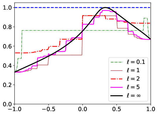
Figure 4: Effect of finite thresholds on the estimator $\hat{s}_{\rm FPR}$ (part I). The function $\hat{s}_{\rm FPR}/\dot{s}$ is plotted as a function of $\Delta$ for finite values of the thresholds $\ell_{-}=\ell_{+}=\ell$. Parameters are the same as in Fig. 2, except that the thresholds are finite, as given in the legend. The dashed, blue, horizontal line is a guide to the eye that indicates the value $1$ corresponding to optimal inference.

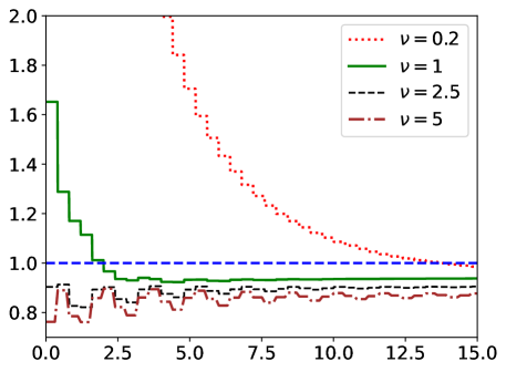
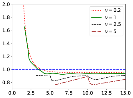
Figure 5: Effect of finite thresholds on the estimator $\hat{s}_{\rm FP}$ (part II). The ratio $\hat{s}_{\rm FPR}/\dot{s}$ is plotted as a function of $\ell_{-}$ (top) and $|\ln p_{-}|$ (bottom) for the current $J$ with $\Delta=0.6$ (defined in Eq. (53)) in the random walk process on a two-dimensional lattice. The rates $k^{+}_{1}$, $k^{-}_{1}$, $k^{+}_{2}$, and $k^{-}_{2}$ are parametrised according to Eqs. (48) and (49), with $\rho=2$ and $\nu=0.2,1,2.5,5$, as given in the legend; the corresponding values of $\dot{s}/k_{\rm total}$ are $0.05$, $1$, $3.5$, and $7.5$, respectively. The thresholds are symmetric, $\ell_{-}=\ell_{+}$. The blue, horizontal, dashed line is a guide to the eye that indicates the value $1$.

In Fig. 5, we analyse $\hat{s}_{\rm FPR}(\ell_{-},\ell_{+})$ as a function of $\ell$ for a fixed value of $\Delta=0.6$; note that this is a generic example for which $J$ is not proportional to $S$, and hence $\hat{s}_{\rm FPR}$ does not capture all the dissipation in the process, not even in the limit of large thresholds. The top panel of Fig. 5 plots $\hat{s}_{\rm FPR}(\ell_{-},\ell_{+})/\dot{s}$ as a function of $\ell$ for different values of $\nu$, which is the parameter that determines the hopping rates according to Eqs. (48) and (49). At large values $\nu\gg 1$ the rate of dissipation is large, and at small values $\nu\approx 0$ the system is almost at equilibrium. In Fig. 5, we observe that asymptotically for large $\ell$, $\hat{s}_{\rm FPR}(\ell_{-},\ell_{+})/\dot{s}<1$, in accordance with the universal first-passage bound (26). However, how fast $\hat{s}_{\rm FPR}(\ell_{-},\ell_{+})/\dot{s}$ converges to its asymptotic limit depends on $\nu$: near equilibrium, e.g., for $\nu=0.2$, large values of $\ell\approx 15$ are required to estimate $\dot{s}$ accurately, while far from thermal equilibrium, e.g., for $\nu>2.5$, the ratio $\hat{s}_{\rm FPR}$ captures about 90% of the dissipation for any value of $\ell$. Hence, for systems far from thermal equilibrium, $\hat{s}_{\rm FPR}$ estimates dissipation well, even at very small values of the thresholds.

In order to better understand what value of $\ell$ is required to estimate dissipation, we plot in the bottom panel of Fig. 5 the ratio $\hat{s}_{\rm FPR}(\ell_{-},\ell_{+})/\dot{s}$ as a function of $|\ln p_{-}|$. This figure shows that $\hat{s}_{\rm FPR}(\ell_{-},\ell_{+})$ estimates well the entropy production rate whenever $|\ln p_{-}|>3$, and hence the relevant asymptotic parameter is $p_{-}$, rather than the threshold value $\ell$. Accordingly, for systems near equilibrium, a large threshold is needed to bring $p_{-}<0.05=e^{-3}$, while for systems far from thermal equilibrium $p_{-}<0.05=e^{-3}$ is reached for any value of the thresholds, as described by Eq. (33).

4.4 Effect of a finite number of realisations

So far, we have analysed $\hat{s}_{\rm FPR}(\ell_{-},\ell_{+})$, which is the value of the estimator $\mathcal{F}_{\rm FPR}$ when an infinite number of realisations are available. However, in experimental situations, we have to deal with a finite amount of data, and hence it is crucial to understand how fast $\mathcal{F}_{\rm FPR}$ converges to $\hat{s}_{\rm FPR}(\ell_{-},\ell_{+})$ as a function of $n_{\rm s}$, the number of realisations of the process $X$. We address this question here by simulating the process $X$ with a continuous-time Monte Carlo algorithm..

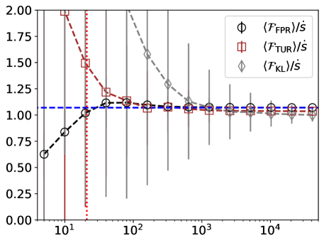
(a) $\nu=0.2$

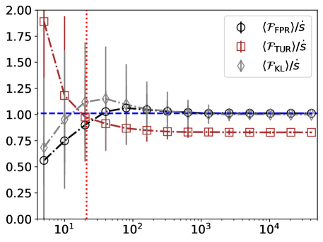
(b) $\nu=1$

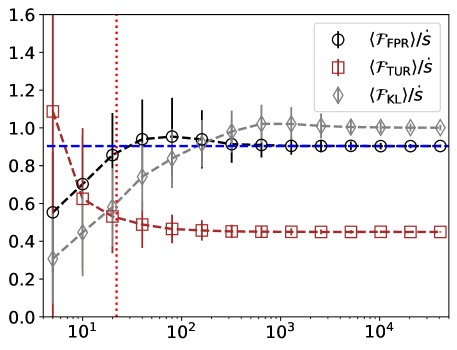
(c) $\nu=2.5$

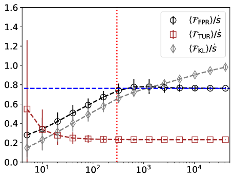
(d) $\nu=5$

Figure 6: Effect of the sample size $n_{\rm s}$ on the bias of estimators of dissipation. Circles, squares, and diamonds denote, respectively, the expected values of $\langle\mathcal{F}_{\rm FRP}\rangle$, $\langle\mathcal{F}_{\rm TUR}\rangle$ and $\langle\mathcal{F}_{\rm KL}\rangle$ ; error bars denote the standard deviations of $\mathcal{F}_{\rm FRP}$ and $\mathcal{F}_{\rm TUR}$. Results shown are for the current $J$ with $\Delta=0.6$ in the random walk process on a two-dimensional lattice. Different figures represent different values of $\nu$, corresponding with increasingly large rates of dissipation, ranging from $\dot{s}=0.05k_{\rm total}$ when $\nu=0.2$ to $\dot{s}=7.5k_{\rm total}$ when $\nu=5$. The same parameters have been selected as in Fig. 5, albeit for a fixed threshold $\ell_{-}=\ell_{+}=\ell$. The thresholds are set at $\ell=10.41,1.61,0.01,0.01$ for $\nu=0.2,1,2.5,5$, respectively, and the TUR and the Kullback-Leibler divergence are evaluated at $t=1/k_{\rm total}$. Markers are empirical averages over $1{\rm e}+3$ runs, each consisting of $n_{\rm s}$ simulated realisations of $X$. The horizontal, blue, dashed lines denote $\hat{s}_{\rm FRP}/\dot{s}$, and the vertical, red, dotted lines denote the value $n_{s}=1/p_{-}$.

Figure 6 shows $\mathcal{F}_{\rm FPR}/\dot{s}$ as a function of $n_{s}$ for the same parameters as in Fig. 5 and for a fixed value of $\ell$. The value of $\ell$ is set to the smallest threshold value so that $p_{-}<0.05$, in particular, $\ell=10.41,1.61,0.01,0.01$ for $\nu=0.2,1,2.5,5$, respectively; note that for $\nu=2.5$ and $\nu=5$, we have set $\ell=0.01$, as setting $\ell=0$ would terminate the process immediately.

We observe two regimes in Fig. 6: (a) when $n_{\rm s}<1/p_{-}$, then $\langle\mathcal{F}_{\rm FPR}\rangle$ grows logarithmically in $n_{\rm s}$; (b) when $n_{\rm s}>1/p_{-}$, then $\langle\mathcal{F}_{\rm FPR}\rangle$ saturates to its asymptotic value $\hat{s}_{\rm FPR}$. To make it easier to differentiate these two regimes, Fig. 6 shows the value $n_{\rm s}=1/p_{-}$ with the vertical dotted lines. Hence, we conclude that, in correspondence with Eq. (30), a number $n_{\rm s}\sim 1/p_{-}$ of samples are required to optimally estimate the rate of dissipation. The saturation of $\langle\mathcal{F}_{\rm FPR}\rangle$ at $n_{\rm s}\sim 1/p_{-}$ has the following intuitive explanation: to determine the magnitude of $p_{-}$, it is necessary to observe the frequency of events that hit the negative threshold first. In the regime $n_{\rm s}\ll/p_{-}$ the experimenter does not observe events for which the current hits the negative threshold first, while for $n_{\rm s}\gg/p_{-}$ the experimenter observes several such events.

Comparing estimates of dissipation based on the FPR with those based on the TUR, we observe that for small values of $\nu$ (or $\dot{s}$) both estimators are equivalent: their asymptotic values for $n_{\rm s}\gg 1$ are almost identical, in correspondence with Fig. 3, and the estimators converge equally fast to the asymptotic limit, viz., about $n_{\rm s}\sim 10^{2}$ realisations are required. On other hand, for large values of $\nu$ (or $\dot{s}$), the FPR captures asymptotically a finite fraction of the entropy production rate, while the TUR captures a negligible fraction of the entropy production rate. However, the small bias of the FPR comes at the expense of a large sample size $n_{\rm s}$ that is required to reach the asymptotic limit (about $n_{\rm s}\sim 10^{3}$ realisations are required for the FPR compared to $n_{\rm s}\sim 30$ for the TUR).

Comparing estimations of dissipation based on $\mathcal{F}_{\rm FPR}$ with those based on $\mathcal{F}_{\rm KL}$, we observe that the bias in $\mathcal{F}_{\rm KL}$ is smaller than the bias in $\mathcal{F}_{\rm FPR}$. This is because in the present model the current is Markovian, and consequently the estimator $\mathcal{F}_{\rm KL}$ is unbiased. However, the dependence on $n_{\rm s}$ is similar for both estimators, viz., for large values of $\nu$ the bias grows logarithmically until it reaches its asymptotic value.

Taken together, Fig. 6 confirms the Eq. (30), and hence although far from thermal equilibrium the FPR estimates a finite fraction of the total dissipation, this comes at the expense of a possibly large number of samples $n_{\rm s}\gtrsim 1/p_{-}$, depending on how small the splitting probability $p_{-}$ is.

5 Inference of the efficiency of molecular motors

As an application, we use first-passage processes to estimate the efficiency at which a molecular motor converts chemical fuel into mechanical work. We assume that the position of the molecular motor, which we denote by $Y$, is observed. Instead, the internal degrees of freedom, such as the chemical states of the motor heads, are not known, and hence this is a problem with partial information. Moreover, in this example the observed current $Y$ is nonMarkovian, and hence with this model we can quantify the influence of nonMarkovian statistics on entropy production estimates. In particular, it will be interesting to compare the biases of $\mathcal{F}_{\rm FPR}$ and $\mathcal{F}_{\rm KL}$.

5.1 General setup: dissipation and efficiency of molecular motors

Consider a molecular motor that moves on a one-dimensional biofilament at mean velocity $v$ in steps of length $\delta$. We denote by $f_{\rm mech}$ the mechanical load felt by the molecular motor ($f_{\rm mech}>0$ denotes a hindering load, while $f_{\rm mech}<0$ is an assisting load). When $f_{\rm mech}v>0$, then the molecular motor consumes chemical fuel in the hydrolysis of adenosine triphosphate (ATP) into adenosine diphopshate (ADP) and an inorganic phosphate (P) to perform work on an external cargo. Following [18], we define the efficiency of the molecular motor as the ratio

$$\eta:=\frac{f_{\rm mech}v}{\dot{w}_{\rm chem}},$$ (65)

between the output power $f_{\rm mech}v$ and the rate $\dot{w}_{\rm chem}$ of consumption of free energy input due to the hydrolysis of ATP into ADP and P.

The rate of dissipation is the sum of the rate of entropy change in the chemostats, given by $\dot{w}_{\rm chem}/\mathsf{T}_{\rm env}$, and in the thermal reservoir, given by $-f_{\rm mech}v/\mathsf{T}_{\rm env}$, viz.,

$$\dot{s}=\frac{\dot{w}_{\rm chem}}{\mathsf{T}_{\rm env}}-\frac{f_{\rm mech}v}{\mathsf{T}_{\rm env}}.$$ (66)

Combining the Eqs. (65) and (66), we obtain the relation

$$\dot{s}=\frac{f_{\rm mech}v}{\mathsf{T}_{\rm env}}\left(\frac{1-\eta}{\eta}\right)$$ (67)

between the rate of dissipation $\dot{s}$ and the motor efficiency.

5.2 A back-of-the-envelope estimate of the efficiency of molecular motors with first-passage processes

Combining the FPR-inequality Eq. (29) with the expression (67), we obtain the upper bound

$$\eta\leq\eta_{\rm FPR}=\left(1+\frac{\mathsf{T}_{\rm env}}{f_{\rm mech}v}\frac{\ell_{+}}{\ell_{-}}\frac{\left|\ln p_{-}\right|}{\langle T_{Y}\rangle}(1+o_{\ell_{\rm min}}(1))\right)^{-1},$$ (68)

on the efficiency of a molecular motor. The bound Eq. (68) is the FPR equivalent of the bound [18],

$$\eta\leq\eta_{\rm TUR}=\left(1+\frac{\mathsf{T}_{\rm env}}{f_{\rm mech}\delta}\frac{2\langle Y(t)\rangle}{\sigma^{2}_{Y(t)}}\right)^{-1}$$ (69)

that follows from the TUR inequality, given by Eq. (38). Analogously, there is the bound

$$\eta\leq\eta_{\rm KL}=\left(1+\frac{\mathsf{T}_{\rm env}}{f_{\rm mech}v}\left(\overline{j}_{\rm f}-\overline{j}_{\rm b}\right)\log\frac{\overline{j}_{\rm f}}{\overline{j}_{\rm b}}\right)^{-1}$$ (70)

based on the Kullback-Leibler divergence.

We estimate $\eta_{\rm FPR}$ based on the experimental data for Kinesin-1 published in Ref. [42]. For forces $f_{\rm mech}=3\>{\rm pN}$ and $[{\rm ATP}]=10\>\mu{\rm M}$, a number of 2-8% of backward steps were observed [42]. Hence, if we set the thresholds $\ell_{-}=\ell_{+}=\delta=8\>{\rm nm}$, then $p_{-}\sim 0.02$, and we are in the asymptotic regime of $p_{-}\lesssim 0.05$ that was identified in Fig. 5(b), albeit for a different model. Setting $\langle T_{Y}\rangle\approx\delta/v$, with $\delta=8{\rm nm}$ the step size of the molecular motor, and considering room temperatures $\mathsf{T}_{\rm env}=298\times 1.38\times 10^{-23}{\rm J}$, we obtain

$$\eta\leq\eta_{\rm FPR}=\frac{1}{1+\frac{298\times 1.38\times 0.01}{24}\times\left|\ln 0.02\right|}\approx 0.6.$$ (71)

As this simple back-of-the-envelope calculation illustrates, we can estimate dissipation in nonequilibrium processes with $\hat{s}_{\rm FPR}$. In the following sections, we use a more detailed analysis that relies on a model for Kinesin-1 dynamics to determine the accuracy of this estimate.

5.3 Model for molecular motors with two motor heads

In the previous section, we have used the FPR to estimate the rate of dissipation of a Kinesin-1 motor. In this section, we consider a molecular motor model for Kinesin-1 to determine the accuracy of this estimate.

We describe the dynamics of Kinesin-1 with a model for two-headed molecular motors. This model is a Markov jump process that determines the transitions between the chemical states of the motor heads, and the model includes also one mechanical step. Each motor head can take three different chemical states, namely, the ADP-bound (${\rm D}$), ATP-bound (${\rm T}$), and nucleotide-free APO states ($\phi$), leading to nine possible states. However, since the kinetics of the two heads are coordinated, see Refs. [22, 6], a six state model with the states

$$X(t)\in\left\{({\rm D}:\phi),({\rm T}:\phi),({\rm T}:D),(\phi:{\rm D}),(\phi:{\rm T}),({\rm D}:{\rm T})\right\}$$ (72)

suffices to describe the dynamics of two-headed molecular motors. For convenience, we also number the states from $1$ to $6$, as shown in Fig. 1(b).

In Fig. 1(b) we show all the possible chemical/mechanical transitions in the six-state model for two-headed molecular motors. As argued in Ref. [22], the mechanical step, corresponding with the interchange of the front and rear head, takes place during the transition from $({\rm D}:{\rm T})$ to $({\rm T}:{\rm D})$, and therefore the position of the motor equals the current

$$Y(t):=J_{2\rightarrow 5}(t),$$ (73)

where for convenience we have set $Y(0)=0$.

The model contains three cycles: a forward cycle at rate $\overline{j}_{\rm f}$ corresponding to an ATP-hydrolysis-induced forward step, a backward cycle at rate $\overline{j}_{\rm b}$ corresponding to an ATP-hydrolysis-induced backward step, and a third cycle with rate $\overline{j}_{0}$ that hydrolysis two ATP molecules but does not change the position of the motor. The total rate of dissipation is

$$\dot{s}=\overline{j}_{\rm f}\frac{a_{\rm f}}{\mathsf{T}_{\rm env}}+\overline{j}_{\rm b}\frac{a_{\rm b}}{\mathsf{T}_{\rm env}}+\overline{j_{0}}\frac{a_{0}}{\mathsf{T}_{\rm env}}$$ (74)

where

$$\frac{a_{\rm f}}{\mathsf{T}_{\rm env}}=\ln\frac{k_{1\rightarrow 2}k_{2\rightarrow 5}k_{5\rightarrow 6}k_{6\rightarrow 1}}{k_{1\rightarrow 6}k_{6\rightarrow 5}k_{5\rightarrow 2}k_{2\rightarrow 1}}=\frac{\Delta\mu}{\mathsf{T}_{\rm env}}-\frac{f_{\rm mech}\delta}{\mathsf{T}_{\rm env}},$$ (75)

$$\frac{a_{\rm b}}{\mathsf{T}_{\rm env}}=\ln\frac{k_{2\rightarrow 3}k_{3\rightarrow 4}k_{4\rightarrow 5}k_{5\rightarrow 2}}{k_{2\rightarrow 5}k_{5\rightarrow 4}k_{4\rightarrow 3}k_{3\rightarrow 2}}=\frac{\Delta\mu}{\mathsf{T}_{\rm env}}+\frac{f_{\rm mech}\delta}{\mathsf{T}_{\rm env}},$$ (76)

are the affinities of the forward and backward cycles, and

$$a_{0}=a_{\rm f}+a_{\rm b}$$ (77)

is the affinity of the third cycle. Here

$$\Delta\mu=\mathsf{T}_{\rm env}\ln\left(K_{\rm eq}\frac{[{\rm ATP}]}{[{\rm ADP}][{\rm P}]}\right)$$ (78)

is the supplied chemical energy due to the hydrolysis of ATP into ADP and P, and $f_{\rm mech}\delta$ is the mechanical work done by the system on an external cargo during one molecular motor step of length $\delta$. In Eq. (78), [ATP], [ADP], and [P], are the concentrations in the surrounding chemostat of ATP, ADP, and P, respectively, and $K_{\rm eq}$ is the equilibrium constant of the hydrolysis reaction.

Following [22, 6], we use for the rates of the chemomechanical transitions between states $2$ and $5$ the formulae

$$k_{2\rightarrow 5}(f_{\rm mech})=k_{2\rightarrow 5}(0)e^{-\theta\frac{f_{\rm mech}\delta}{\mathsf{T}_{\rm env}}}$$ (79)

and

$$k_{5\rightarrow 2}(f_{\rm mech})=k_{5\rightarrow 2}(0)e^{(1-\theta)\frac{f_{\rm mech}\delta}{\mathsf{T}_{\rm env}}}.$$ (80)

For the other rates we set

$$k_{i\rightarrow j}(f_{\rm mech})=\frac{2k_{i\rightarrow j}(0)}{1+e^{\chi_{ij}\frac{f_{\rm mech}\delta}{\mathsf{T}_{\rm env}}}}$$ (81)

with $\chi_{ij}=\chi_{ji}$. The concentration $[{\rm ATP}]$ determines the rates

$$k_{1\rightarrow 2}(0)=k^{\rm bi}_{1\rightarrow 2}[{\rm ATP}]$$ (82)

and

$$k_{4\rightarrow 5}(0)=k^{\rm bi}_{4\rightarrow 5}[{\rm ATP}],$$ (83)

and the explicit dependence on the concentrations $[{\rm ADP}]$ and $[{\rm P}]$ is not considered. Due to the equivalence of the two cycles, we also set $k_{3\rightarrow 2}(0)=k_{6\rightarrow 5}(0)$, $k_{2\rightarrow 3}(0)=k_{5\rightarrow 6}(0)$, $k_{3\rightarrow 4}(0)=k_{6\rightarrow 1}(0)$, $k_{4\rightarrow 3}(0)=k_{1\rightarrow 6}(0)$, $k_{4\rightarrow 5}(0)=k_{1\rightarrow 2}(0)$, $\chi_{23}=\chi_{56}$, $\chi_{34}=\chi_{61}$, and $\chi_{45}=\chi_{12}$. Moerover, we set

$$k_{5\rightarrow 2}(0)=k_{2\rightarrow 5}(0)\sqrt{\frac{k_{5\rightarrow 4}(0)}{k_{2\rightarrow 1}(0)}},$$ (84)

such that the six-state model satisfies detailed balance when

$$f_{\rm mech}=0\quad{\rm and}\quad[{\rm ATP}]=\frac{k_{1\rightarrow 6}(0)}{k_{6\rightarrow 1}(0)}\frac{k_{6\rightarrow 5}(0)}{k_{5\rightarrow 6}(0)}\frac{\sqrt{k_{5\rightarrow 4}(0)k_{2\rightarrow 1}(0)}}{k^{\rm bi}_{4\rightarrow 5}}.$$ (85)

For these values of the control parameters, there is neither a chemical driving force ($\Delta\mu=0$) nor a mechanical force ($f_{\rm mech}=0$).

The remaining parameters $k_{i\rightarrow j}(0)$, $\theta$, $\chi_{ij}$, $k^{\rm bi}_{1\rightarrow 2}$, and $k^{\rm bi}_{4\rightarrow 5}$ are motor specific, and for Kinesin-1 they have been obtained in Refs. [6, 7] from fitting single molecule motility data to the six-state model. Here, we will use these fitted parameters for Kinesin-1, and for convenience we summarise the exact numerical values in C.

The concentration $[{\rm ATP}]$ and the mechanical load $f_{\rm mech}\delta/\mathsf{T_{\rm env}}$ are external, control parameters that can be modified by the experimenter.

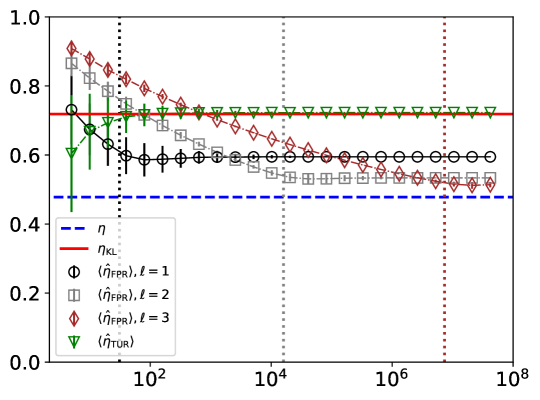
Figure 7: Simulation results for estimated molecular motor efficiencies. The estimated efficiencies $\langle\hat{\eta}_{\rm FPR}\rangle$, based on first-passage processes for the position $Y(t)$ in the molecular motor model described in Sec. 5.3, as a function of the number of realisations $n_{\rm s}$ for three different values of the thresholds $\ell_{-}=\ell_{+}=\ell$ (as indicated by the legend), $[\rm ATP]=10\mu{\rm M}$, and $f_{\rm mech}=3{\rm pN}$. For reference, the efficiency $\eta=4.78$ is shown with the horizontal, blue dashed line; the estimate $\eta_{\rm KL}$ based on the Kullback-Leibler divergence in the limit of $n_{\rm s}\gg 1$ is shown by the horizontal, red, solid line; and the estimates $\langle\hat{\eta}_{\rm TUR}\rangle$ based on the TUR evaluated at $t=1{\rm s}$ are shown by the green triangles. Each marker is an average over $1000$ or $100$ (for large values of $n_{\rm s}$) realisations and the error bars denote the standard deviations of $\hat{\eta}_{\rm FPR}$ and $\hat{\eta}_{\rm TUR}$. The vertical, dotted lines denote the values of $n_{\rm s}=1/p_{-}$.

5.4 Estimating the efficiency of a molecular motor based on the measurement of its position

We estimate the efficiency $\eta$ from the measurement of the position $Y$ of the molecular motor, which according to Eq. (67) is equivalent to an entropy production estimation problem. We consider the case of $[{\rm ATP}]=10\mu{\rm M}$ and $f_{\rm mech}=3{\rm pN}$, corresponding with the calculation in Sec. 5.2 based on experimental data.

We define two estimators $\hat{\eta}_{\rm FPR}$, and $\hat{\eta}_{\rm TUR}$ for the efficiency of $\eta$ that are equivalent to the estimators $\mathcal{F}_{\rm FPR}$ and $\mathcal{F}_{\rm TUR}$ for the rate of dissipation, i.e., they are estimates for the efficiency when a finite number of trajectories are available. For estimation based on first-passage processes, we consider

$$\hat{\eta}_{\rm FPR}:=\left(1+\frac{\mathsf{T}_{\rm env}}{f_{\rm mech}v}\frac{\ell_{+}}{\ell_{-}}\frac{\left|\ln\hat{p}_{-}\right|}{\langle\hat{T}_{Y}\rangle}\right)^{-1},$$ (86)

where $\hat{p}_{-}$ and $\hat{T}_{Y}$ are the estimates of $p_{-}$ and $\langle T_{Y}\rangle$ based on a finite number of realisations of the process, as in Eqs. (24) and (25); note that we assume that $v=\delta\langle Y(t)\rangle/t$ is known, although we could also take an estimated value for this quantity leading to almost identical results. To estimate the motor efficiency based on the TUR, we use

$$\hat{\eta}_{\rm TUR}:=\left(1+\frac{\mathsf{T}_{\rm env}}{f_{\rm mech}\delta\>}\frac{2\hat{Y}(t)}{\hat{\sigma}^{2}_{Y(t)}}\right)^{-1},$$ (87)

where $\hat{Y}(t)=n_{\rm s}^{-1}\sum^{n_{\rm s}}_{i=1}Y^{(i)}(t)$ and $\hat{\sigma}^{2}_{Y(t)}=n^{-1}_{\rm s}\sum^{n_{\rm s}}_{i=1}\left(Y^{(i)}(t)\right)^{2}-n^{-2}_{\rm s}\left(\sum^{n_{\rm s}}_{i=1}Y^{(i)}(t)\right)^{2}$.

Figure 7 plots $\langle\hat{\eta}_{\rm FPR}\rangle$ as a function of $n_{\rm s}$ for three values of $\ell=\ell_{-}=\ell_{+}$, namely, $\ell=1$, $\ell=2$, and $\ell=3$, and compares the estimate $\langle\hat{\eta}_{\rm FPR}\rangle$ with the efficiency $\eta=0.478$ and the estimate $\langle\hat{\eta}_{\rm TUR}\rangle$ based on the TUR.

Just as for the $\mathcal{F}_{\rm FPR}$ in Fig. 6, we can differentiate two regimes: (i) for $n_{s}<1/p_{-}$, the estimator $\langle\hat{\eta}_{\rm FPR}\rangle$ decreases logarithmically; and (ii) for $n_{s}>1/p_{-}$, the estimator $\langle\hat{\eta}_{\rm FPR}\rangle$ has reached its asymptotic value. The values $n_{\rm s}=1/p_{-}$ that separate the two regimes are indicated for different values of $\ell$ by the vertical dotted lines.

For $\ell=1$, $\langle\hat{\eta}_{\rm FPR}\rangle$ converges to its asymptotic value $0.6$, which is similar to the value we estimated in Sec. 5.2 based on experimental data. The simulation results in Fig. 7 show that this estimate can be improved by considering larger values of $\ell$, but this comes at a significant expense in the number of realisations $n_{s}$ required. Nevertheless, the estimate $\langle\hat{\eta}_{\rm FPR}\rangle$ at small thresholds $\ell=1$ is better than the estimate $\langle\hat{\eta}_{\rm TUR}\rangle$, indicating again that small thresholds are sufficient to obtain accurate estimates of dissipation with FPRs.

Interestingly, Fig. 7 shows that the estimates $\langle\hat{\eta}_{\rm FPR}\rangle$ are less biased than the estimate $\eta_{\rm KL}$, given by Eq. (70), based on the Kullback-Leibler divergence. Note that in the present example $Y$ is a nonMarkovian current. Since $\eta_{\rm KL}$ does not account for nonMarkovian effects in the current, we can attribute the smaller bias in the FPR due to the nonMarkovian statistics of $Y$ that are accounted for by the FPR.

6 Discussion

We have studied the problem of inferring the rate of entropy production $\dot{s}$ from the measurement of repeated realisations of a first-passage process of a single current. To this aim, we have used the estimator $\mathcal{F}_{\rm FPR}$ [Eq. (23)] that converges in the limit of an infinite number of realisations of the process to the first-passage ratio $\hat{s}_{\rm FPR}$ [Eq. (3)]. We have compared this estimator with $\mathcal{F}_{\rm TUR}$, an estimator based on the TUR, and with $\mathcal{F}_{\rm KL}$, an estimator based on the Kullback-Leibler divergence. We discuss now the strengths and weakness of these different estimators, and we also provide an outlook on future challenges.

Comparing $\mathcal{F}_{\rm FPR}$ with $\mathcal{F}_{\rm TUR}$, we conclude that far from thermal equilibrium the FPR is a better estimator of dissipation. Indeed, as shown in Fig. 3, far from thermal equilibrium the FPR captures a finite fraction of $\dot{s}$, while the TUR captures a negligible fraction $\dot{s}$; note that in the literature modifications of the TUR have been derived that have a smaller bias than $\hat{s}_{\rm TUR}$ [38, 39], but these modified TURs rely on measurements of both currents and time-integrated empirical measures, and hence require more information about the process $X$ than the trajectories of a single current. The estimation of dissipation with $\hat{s}_{\rm FPR}$ does require a number $n_{\rm s}\gg 1/p_{-}$ of realisations of the nonequilibrium process, which can be large for processes far from thermal equilibrium; in particular, we have shown that the number of realisations $n_{\rm s}$ increases exponentially as a function of $\Delta s$, the minimal jump size of $S$. Nevertheless, since far from thermal equilibrium $\mathcal{F}_{\rm TUR}/\dot{s}\approx 0$, it holds that the bias of the FPR is smaller than the bias of the TUR, even for values of $n_{\rm s}$ that are smaller than $1/p_{-}$.

Comparing $\mathcal{F}_{\rm FPR}$ with $\mathcal{F}_{\rm KL}$, we conclude that for generic Markov jump processes the bias in $\mathcal{F}_{\rm FPR}$ is smaller than the bias in $\mathcal{F}_{\rm KL}$, as the FPR captures nonMarkovian effects in the current (see Fig. 7). An exception is when the current $J$ is Markovian, as was the case for the random walk process discussed in Sec. 4. Note that it is possible to include memory effects in the Kullback-Leibler divergence, e.g., by assuming the current is a semi-Markov process [14], but in general this still leads to a biased estimator of dissipation

Taken together, the three estimators $\mathcal{F}_{\rm FPR}$, $\mathcal{F}_{\rm TUR}$, and $\mathcal{F}_{\rm KL}$ are valid estimators of dissipation, as they can be used to estimate dissipation in different circumstances. Near equilibrium and with limited data available, the TUR is a good estimator of dissipation; for Markovian currents the Kullback-Leibler divergence is the best estimator; and for processes far from equilibrium with nonMarkovian currents the FPR is the estimator with the least bias.

In the present paper, we have considered entropy production estimation based on the measurement of a single current. Since all estimators are bounded from above by the rate $\dot{s}$ of entropy production, we can reduce the bias in the estimators by measuring multiple currents, and maximising the estimator towards linear combinations of these currents. In this regard, the FPR has the appealing property that the maximum of this variational problem is attained by a current that is proportional to the entropy production, and hence the affinities of the process can be inferred from a variational principle.

The purpose of the present paper was to highlight the potential of a first-passage approach to the entropy-production estimation problem. To this aim, we have performed a comparative study using two simple examples of nonequilibrium processes. However, to better understand estimation theory for entropy production rates, we think it will be important to take the present study one step further and make an extensive comparison of the different methods for the estimation of entropy production used in the literature, e.g., by using a larger pool of estimators for entropy production and a larger pool of models representing nonequilibrium systems. In this regard, one should be careful to make a fair comparison of the different methods based on the knowledge they require about the nonequilibrium process and the amount of data used. Also, we hope the present manuscript highlights the importance of developing further the mathematics underlying the estimator $\hat{s}_{\rm FPR}$ through extensions of the results in Ref. [2].

We end the paper with the discussion of an interesting, potential application in cell biology. Proteins in living cells produce entropy, as they are involved in chemical reactions that operate far from chemical equilibrium. However, due to the diffraction limit, it is challenging to measure the trajectories of individual proteins in living cells at high enough spatial and temporal resolution. Nevertheless, in recent years significant advances have been made in super-resolution live cell imaging, see e.g. Refs. [43, 45, 46]. If the resolution of these imaging methods can be further improved, then it will certainly be possible to infer entropy production rates of individual proteins in living cells from the measurements of their trajectories.

Appendix A Splitting probabilities of $S$

To derive an exact expression for the splitting probabilities $p_{-}$ and $p_{+}$ of $S(t)$, we use the integral fluctuation relation at stopping times [32]

$$\langle e^{-S(T_{J})}\rangle=1,$$ (88)

where $T_{J}$ is a first-passage time of a current $J$ with two thresholds, as defined in Eq. (19). The derivations below follow the Refs. [31, 32].

Since the interval $(-\ell_{-},\ell_{+})$ is finite,

$$\mathbb{P}\left(T_{J}<\infty\right)=1,$$ (89)

and therefore

$$p_{-}+p_{+}=1$$ (90)

and

$$p_{-}\langle e^{-S(T_{J})}|S(T_{J})\leq-\ell_{-}\rangle+p_{+}\langle e^{-S(T_{J})}|S(T_{J})\geq\ell_{+}\rangle=1,$$ (91)

where $\langle\cdot|\cdot\rangle$ are conditional expectations. Equations (90) and (91) imply that

$$p_{-}=\frac{1-\langle e^{-S(T_{J})}|S(T_{J})\geq\ell_{+}\rangle}{\langle e^{-S(T_{J})}|S(T_{J})\leq-\ell_{-}\rangle-\langle e^{-S(T_{J})}|S(T_{J})\geq\ell_{+}\rangle}.$$ (92)

Hence, when the stochastic entropy production $S(t)$ has continuous trajectories — for Markov jump processes this is the near-equilibrium limit — Eq. (92) implies

$$p_{-}=\frac{1-e^{-\ell_{+}}}{e^{\ell_{-}}-e^{-\ell_{+}}}.$$ (93)

On the other hand, when the stochastic entropy production $S(t)$ has jumps — for Markov jump processes this is the general case — this gives

$$p_{-}\leq\frac{1}{e^{\ell_{-}}-e^{-\ell_{+}}}.$$ (94)

In addition, when the depth $\ell_{-}$ of the negative thresholds is small, the bound (94) can be improved. Particularily, defining

$$\Delta s={\rm inf}\left\{|S(t)-\lim_{\epsilon\rightarrow 0^{+}}S(t-\epsilon)|:t\geq 0\right\},$$ (95)

the infimum value of the jump size in $S(t)$, we obtain

$$p_{-}\leq\frac{1}{e^{{\rm max}\left\{\ell_{-},\Delta s\right\}}-e^{-\ell_{+}}}.$$ (96)

Hence, for processes governed far from thermal equilibrium so that $\Delta s\gg 1$, we obtain

$$p_{-}\leq e^{-\Delta s}.$$ (97)

Appendix B Recursion equations for $\langle T_{J}\rangle$ and $p_{-}$ for a random walker on a two-dimensional lattice

We derive a set of recursion equations that determine $\langle T_{J}\rangle$ and $p_{-}$ for currents $J$, as given by Eq. (53), in random walkers on a two-dimensional lattice.

B.1 Recursion equations for $p_{-}$

Let $p_{-}(x_{1},x_{2})$ be the probability for $X=(X_{1},X_{2})$ to reach the region

$$(1-\Delta)X_{1}+(1+\Delta)X_{2}\leq-\ell_{-}$$ (98)

before reaching

$$(1-\Delta)X_{1}+(1+\Delta)X_{2}\geq\ell_{+},$$ (99)

when the initial values $X_{1}(0)=x_{1}$ and $X_{2}(0)=x_{2}$.

Let

$$\mathcal{D}_{-}=\left\{(x,y)\in\mathbb{R}^{2}:(1-\Delta)x+(1+\Delta)y\leq-\ell_{-}\right\}$$ (100)

and

$$\mathcal{D}_{+}=\left\{(x,y)\in\mathbb{R}^{2}:(1-\Delta)x+(1+\Delta)y\geq\ell_{+}\right\}.$$ (101)

It holds for all $(x,y)\notin\mathcal{D}_{-}\cup\mathcal{D}_{+}$ that [47]

$$p_{-}(x,y)=\frac{k^{-}_{1}}{k_{\rm tot}}p_{-}(x-1,y)+\frac{k^{+}_{1}}{k_{\rm tot}}p_{-}(x+1,y)+\frac{k^{-}_{2}}{k_{\rm tot}}p_{-}(x,y-1)+\frac{k^{+}_{2}}{k_{\rm tot}}p_{-}(x,y+1),$$

(102)

where $k_{\rm tot}=k^{+}_{1}+k^{-}_{1}+k^{+}_{2}+k^{-}_{2}$, and with boundary conditions

$$p_{-}(x,y)=1\quad{\rm if}\quad(x,y)\in\mathcal{D}_{-}$$ (103)

and

$$p_{-}(x,y)=0\quad{\rm if}\quad(x,y)\in\mathcal{D}_{+}.$$ (104)

The Eqs. (102-104) admit a unique solution $p_{-}(x,y)$ [47], which can be found by solving the iterative equations

$$p_{-}(x,y;n)=\frac{k^{-}_{1}}{k_{\rm tot}}p_{-}(x-1,y;n-1)+\frac{k^{+}_{1}}{k_{\rm tot}}p_{-}(x+1,y;n-1)$$

$$+\frac{k^{-}_{2}}{k_{\rm tot}}p_{-}(x,y-1;n-1)+\frac{k^{+}_{2}}{k_{\rm tot}}p_{-}(x,y+1;n-1),$$ (105)

for $(x,y)\in\mathbb{R}^{2}\setminus\mathcal{D}^{-}\cup\mathcal{D}^{+}$ and $n\in\mathbb{N}$, and with boundary conditions

$$p_{-}(x,y;n)=1\quad{\rm if}\quad(x,y)\in\mathcal{D}_{-}$$ (106)

and

$$p_{-}(x,y;n)=0\quad{\rm if}\quad(x,y)\in\mathcal{D}_{+},$$ (107)

also for $n\in\mathbb{N}$. In the limit of large $n$, the stationary solution to the Eqs. (105-107) converges to the solution of (102-104).

B.2 Recursion equations for $\langle T_{J}\rangle$

The mean first-passage time $t(x,y)=\langle T_{J}|X(0)=x,Y(0)=y\rangle$ solves for all $(x,y)\notin\mathcal{D}_{-}\cup\mathcal{D}_{+}$ the equations [47]

$$t(x,y)=\frac{k^{-}_{1}}{k_{\rm tot}}t(x-1,y)+\frac{k^{+}_{1}}{k_{\rm tot}}t(x+1,y)+\frac{k^{-}_{2}}{k_{\rm tot}}t(x,y-1)+\frac{k^{+}_{2}}{k_{\rm tot}}t(x,y+1)+1$$ (108)

and with boundary conditions

$$t(x,y)=0\quad{\rm if}\quad(x,y)\in\mathcal{D}_{-}$$ (109)

and

$$t(x,y)=0\quad{\rm if}\quad(x,y)\in\mathcal{D}_{+}.$$ (110)

Just as before, we can solve these equations iteratively by introducing a time-index

$$t(x,y;n)=\frac{k^{+}_{1}}{k_{\rm tot}}t(x-1,y;n-1)+\frac{k^{-}_{1}}{k_{\rm tot}}t(x+1,y;n-1)$$

$$+\frac{k^{+}_{2}}{k_{\rm tot}}t(x,y-1;n-1)+\frac{k^{-}_{2}}{k_{\rm tot}}t(x,y+1;n-1)+\frac{1}{k_{\rm tot}},$$ (111)

for $(x,y)\in\mathbb{R}^{2}\setminus\mathcal{D}^{-}\cup\mathcal{D}^{+}$ and $n\in\mathbb{N}$, and with

$$t(x,y;n)=0\quad{\rm if}\quad(x,y)\in\mathcal{D}_{-}$$ (112)

and

$$t(x,y;n)=0\quad{\rm if}\quad(x,y)\in\mathcal{D}_{+},$$ (113)

also for all $n\in\mathbb{N}$.

Appendix C Parameters used for the six-state model of Kinesin-1

We specify the parameters that we use in Sec. 5 for the six-state model for two-headed molecular motors, as visualised in Fig. 1.

The rates are parametrised as in Eqs. (79), (80), and (81), and we thus need to specify the $k_{i\rightarrow j}(0)$, $\theta$, and $\chi_{ij}$. All parameters, except for $k_{5\rightarrow 2}(0)$, are set identical as those in Ref. [6], which were obtained by fitting numerical result to single molecule motility data. In particular we set $\theta=0.61$, $\chi_{12}=0.15$, $\chi_{56}=0.0015$, $\chi_{61}=0.11$, $k_{2\rightarrow 1}(0)=4200\>s^{-1}$, $k_{2\rightarrow 5}(0)=1.6\times 10^{6}\>s^{-1}$,$k_{5\rightarrow 6}(0)=190\>s^{-1}$, $k_{6\rightarrow 5}(0)=10\>s^{-1}$, $k_{6\rightarrow 1}(0)=250\>s^{-1}$, $k_{1\rightarrow 6}(0)=230\>s^{-1}$, $k_{5\rightarrow 4}(0)=2.1\times 10^{-9}\>s^{-1}$, and we set $k_{1\rightarrow 2}(0)=k^{\rm bi}_{1\rightarrow 2}(0)[{\rm ATP}]$ with $k^{\rm bi}_{1\rightarrow 2}(0)=2.8\>\mu M^{-1}s^{-1}$. Note that due to the equivalence of the two cycles, we have set $k_{3\rightarrow 2}=k_{6\rightarrow 5}$, $k_{2\rightarrow 3}=k_{5\rightarrow 6}$, $k_{3\rightarrow 4}=k_{6\rightarrow 1}$, $k_{4\rightarrow 3}=k_{1\rightarrow 6}$, $k_{4\rightarrow 5}=k^{\rm bi}_{4\rightarrow 5}[{\rm ATP}]=k_{1\rightarrow 2}=k^{\rm bi}_{1\rightarrow 2}[{\rm ATP}]$, $\chi_{23}=\chi_{56}$, $\chi_{34}=\chi_{61}$, and $\chi_{45}=\chi_{12}$.

For the rate $k_{5\rightarrow 2}(0)$ we have used Eq. (84) instead of the value

$$k_{5\rightarrow 2}(0)=1.1s^{-1}$$ (114)

used in Ref. [6]. The reason we prefer to use Eq. (84) is because then the model satisfies detailed balance when the control parameters are given by Eq. (85). Moreover, since

$$k_{2\rightarrow 5}(0)\sqrt{\frac{k_{5\rightarrow 4}(0)}{k_{2\rightarrow 1}(0)}}\approx 1.13{\rm s}^{-1}$$ (115)

this will make no discernible difference in the model fits.

At equilibrium, i.e. for the control parameters given by Eq. (85), the stationary state is

$$p_{\rm eq}(1)=\frac{1}{\mathcal{N}},\quad p_{\rm eq}(2)=\frac{1}{\mathcal{N}}\sqrt{\frac{k_{5\rightarrow 4}(0)}{k_{2\rightarrow 1}(0)}}\frac{k_{4\rightarrow 3}(0)}{k_{3\rightarrow 4}(0)}\frac{k_{3\rightarrow 2}(0)}{k_{2\rightarrow 3}(0)},\quad p_{\rm eq}(3)=\frac{1}{\mathcal{N}}\sqrt{\frac{k_{5\rightarrow 4}(0)}{k_{2\rightarrow 1}(0)}}\frac{k_{4\rightarrow 3}(0)}{k_{3\rightarrow 4}(0)},$$

$$p_{\rm eq}(4)=\frac{1}{\mathcal{N}}\sqrt{\frac{k_{5\rightarrow 4}(0)}{k_{2\rightarrow 1}(0)}},\quad p_{\rm eq}(5)=\frac{1}{\mathcal{N}}\frac{k_{4\rightarrow 3}(0)}{k_{3\rightarrow 4}(0)}\frac{k_{3\rightarrow 2}(0)}{k_{2\rightarrow 3}(0)},\quad p_{\rm eq}(6)=\frac{1}{\mathcal{N}}\frac{k_{4\rightarrow 3}(0)}{k_{3\rightarrow 4}(0)},$$ (116)

where the normalisation constant is

$$\mathcal{N}=1+\sqrt{\frac{k_{5\rightarrow 4}(0)}{k_{2\rightarrow 1}(0)}}\frac{k_{4\rightarrow 3}(0)}{k_{3\rightarrow 4}(0)}\frac{k_{3\rightarrow 2}(0)}{k_{2\rightarrow 3}(0)}+\sqrt{\frac{k_{5\rightarrow 4}(0)}{k_{2\rightarrow 1}(0)}}\frac{k_{4\rightarrow 3}(0)}{k_{3\rightarrow 4}(0)}$$

$$+\sqrt{\frac{k_{5\rightarrow 4}(0)}{k_{2\rightarrow 1}(0)}}+\frac{k_{4\rightarrow 3}(0)}{k_{3\rightarrow 4}(0)}\frac{k_{3\rightarrow 2}(0)}{k_{2\rightarrow 3}(0)}+\frac{k_{4\rightarrow 3}(0)}{k_{3\rightarrow 4}(0)}.$$ (117)

References

References

- [1] É. Roldán, I. Neri, M. Dörpinghaus, H. Meyr, and F. Jülicher, “Decision making in the arrow of time,” Physical review letters, vol. 115, no. 25, p. 250602, 2015.
- [2] I. Neri, “Universal tradeoff relation between speed, uncertainty, and dissipation in nonequilibrium stationary states,” SciPost Phys., vol. 12, p. 139, 2022.
- [3] H. B. Callen, Thermodynamics and an Introduction to Thermostatistics. John Wiley & Sons, 2nd ed., 1985.
- [4] K. Sekimoto, Stochastic energetics.
- [5] W. Hwang and C. Hyeon, “Quantifying the heat dissipation from a molecular motor’s transport properties in nonequilibrium steady states,” The journal of physical chemistry letters, vol. 8, no. 1, pp. 250–256, 2017.
- [6] W. Hwang and C. Hyeon, “Energetic costs, precision, and transport efficiency of molecular motors,” The journal of physical chemistry letters, vol. 9, no. 3, pp. 513–520, 2018.
- [7] W. Hwang and C. Hyeon, “Correction to “energetic costs, precision, and transport efficiency of molecular motors”,” The journal of physical chemistry letters, vol. 10, no. 12, pp. 3472–3472, 2019.
- [8] A. Zogg, F. Stoessel, U. Fischer, and K. Hungerbühler, “Isothermal reaction calorimetry as a tool for kinetic analysis,” Thermochimica acta, vol. 419, no. 1-2, pp. 1–17, 2004.
- [9] T. Maskow and S. Paufler, “What does calorimetry and thermodynamics of living cells tell us?,” Methods, vol. 76, pp. 3–10, 2015.
- [10] U. Seifert, “From stochastic thermodynamics to thermodynamic inference,” Annual Review of Condensed Matter Physics, vol. 10, pp. 171–192, 2019.
- [11] T. R. Gingrich, G. M. Rotskoff, and J. M. Horowitz, “Inferring dissipation from current fluctuations,” Journal of Physics A: Mathematical and Theoretical, vol. 50, no. 18, p. 184004, 2017.
- [12] A. Gomez-Marin, J. M. Parrondo, and C. Van den Broeck, “Lower bounds on dissipation upon coarse graining,” Physical Review E, vol. 78, no. 1, p. 011107, 2008.
- [13] E. Roldán and J. M. R. Parrondo, “Estimating dissipation from single stationary trajectories,” Phys. Rev. Lett., vol. 105, p. 150607, Oct 2010.
- [14] I. A. Martínez, G. Bisker, J. M. Horowitz, and J. M. Parrondo, “Inferring broken detailed balance in the absence of observable currents,” Nature communications, vol. 10, no. 1, pp. 1–10, 2019.
- [15] É. Roldán, J. Barral, P. Martin, J. M. Parrondo, and F. Jülicher, “Quantifying entropy production in active fluctuations of the hair-cell bundle from time irreversibility and uncertainty relations,” New Journal of Physics, vol. 23, no. 8, p. 083013, 2021.
- [16] J. Ehrich, “Tightest bound on hidden entropy production from partially observed dynamics,” Journal of Statistical Mechanics: Theory and Experiment, vol. 2021, no. 8, p. 083214, 2021.
- [17] P. E. Harunari, A. Dutta, M. Polettini, and É. Roldán, “What to learn from few visible transitions’ statistics?,” arXiv preprint arXiv:2203.07427, 2022.
- [18] P. Pietzonka, A. C. Barato, and U. Seifert, “Universal bound on the efficiency of molecular motors,” Journal of Statistical Mechanics: Theory and Experiment, vol. 2016, no. 12, p. 124004, 2016.
- [19] T. Van Vu, V. T. Vo, and Y. Hasegawa, “Entropy production estimation with optimal current,” Phys. Rev. E, vol. 101, p. 042138, Apr 2020.
- [20] S. K. Manikandan, D. Gupta, and S. Krishnamurthy, “Inferring entropy production from short experiments,” Phys. Rev. Lett., vol. 124, p. 120603, Mar 2020.
- [21] S. Pigolotti, I. Neri, E. Roldán, and F. Jülicher, “Generic properties of stochastic entropy production,” Phys. Rev. Lett., vol. 119, p. 140604, Oct 2017.
- [22] S. Liepelt and R. Lipowsky, “Kinesin’s network of chemomechanical motor cycles,” Phys. Rev. Lett., vol. 98, p. 258102, Jun 2007.
- [23] P. Brémaud, Markov chains: Gibbs fields, Monte Carlo simulation, and queues, vol. 31. Springer Science & Business Media, 2013.
- [24] U. Seifert, “Stochastic thermodynamics, fluctuation theorems and molecular machines,” Reports on Progress in Physics, vol. 75, no. 12, p. 126001, 2012.
- [25] L. Peliti and S. Pigolotti, Stochastic Thermodynamics: An Introduction. Princeton University Press, 2021.
- [26] P. G. Bergmann and J. L. Lebowitz, “New approach to nonequilibrium processes,” Phys. Rev., vol. 99, pp. 578–587, Jul 1955.
- [27] J. Schnakenberg, “Network theory of microscopic and macroscopic behavior of master equation systems,” Rev. Mod. Phys., vol. 48, pp. 571–585, Oct 1976.
- [28] C. Maes and K. Netočnỳ, “Time-reversal and entropy,” Journal of statistical physics, vol. 110, no. 1, pp. 269–310, 2003.
- [29] C. Maes, “Local detailed balance,” SciPost Phys. Lect. Notes, p. 32, 2021.
- [30] R. Chetrite and S. Gupta, “Two refreshing views of fluctuation theorems through kinematics elements and exponential martingale,” Journal of Statistical Physics, vol. 143, no. 3, pp. 543–584, 2011.
- [31] I. Neri, E. Roldán, and F. Jülicher, “Statistics of infima and stopping times of entropy production and applications to active molecular processes,” Phys. Rev. X, vol. 7, p. 011019, Feb 2017.
- [32] I. Neri, É. Roldán, S. Pigolotti, and F. Jülicher, “Integral fluctuation relations for entropy production at stopping times,” Journal of Statistical Mechanics: Theory and Experiment, vol. 2019, no. 10, p. 104006, 2019.
- [33] A. C. Barato and U. Seifert, “Thermodynamic uncertainty relation for biomolecular processes,” Phys. Rev. Lett., vol. 114, p. 158101, Apr 2015.
- [34] T. R. Gingrich, J. M. Horowitz, N. Perunov, and J. L. England, “Dissipation bounds all steady-state current fluctuations,” Phys. Rev. Lett., vol. 116, p. 120601, Mar 2016.
- [35] P. Pietzonka, F. Ritort, and U. Seifert, “Finite-time generalization of the thermodynamic uncertainty relation,” Phys. Rev. E, vol. 96, p. 012101, Jul 2017.
- [36] J. M. Horowitz and T. R. Gingrich, “Proof of the finite-time thermodynamic uncertainty relation for steady-state currents,” Phys. Rev. E, vol. 96, p. 020103, Aug 2017.
- [37] D. M. Busiello and S. Pigolotti, “Hyperaccurate currents in stochastic thermodynamics,” Phys. Rev. E, vol. 100, p. 060102, Dec 2019.
- [38] N. Shiraishi, “Optimal thermodynamic uncertainty relation in markov jump processes,” Journal of Statistical Physics, vol. 185, no. 3, pp. 1–15, 2021.
- [39] A. Dechant and S.-i. Sasa, “Improving thermodynamic bounds using correlations,” Phys. Rev. X, vol. 11, p. 041061, Dec 2021.
- [40] M. Uhl, P. Pietzonka, and U. Seifert, “Fluctuations of apparent entropy production in networks with hidden slow degrees of freedom,” Journal of Statistical Mechanics: Theory and Experiment, vol. 2018, no. 2, p. 023203, 2018.
- [41] D. M. Busiello and C. Fiore, “Hyperaccurate bounds in discrete-state markovian systems,” arXiv preprint arXiv:2205.00294, 2022.
- [42] H. Kojima, E. Muto, H. Higuchi, and T. Yanagida, “Mechanics of single kinesin molecules measured by optical trapping nanometry,” Biophysical journal, vol. 73, no. 4, pp. 2012–2022, 1997.
- [43] M. Fernández-Suárez and A. Y. Ting, “Fluorescent probes for super-resolution imaging in living cells,” Nature reviews Molecular cell biology, vol. 9, no. 12, pp. 929–943, 2008.
- [44] I. Di Terlizzi and M. Baiesi, “Kinetic uncertainty relation,” Journal of Physics A: Mathematical and Theoretical, vol. 52, no. 2, p. 02LT03, 2018.
- [45] M. Lelek, M. T. Gyparaki, G. Beliu, F. Schueder, J. Griffié, S. Manley, R. Jungmann, M. Sauer, M. Lakadamyali, and C. Zimmer, “Single-molecule localization microscopy,” Nature Reviews Methods Primers, vol. 1, no. 1, pp. 1–27, 2021.
- [46] R. Ranjan and X. Chen, “Super-resolution live cell imaging of subcellular structures,” JoVE (Journal of Visualized Experiments), no. 167, p. e61563, 2021.
- [47] P. G. Doyle and J. L. Snell, Random walks and electric networks, vol. 22. American Mathematical Soc., 1984.