Near-Optimal Bounds for Testing Histogram Distributions

Abstract

We investigate the problem of testing whether a discrete probability distribution over an ordered domain is a histogram on a specified number of bins. One of the most common tools for the succinct approximation of data, $k$-histograms over $[n]$, are probability distributions that are piecewise constant over a set of $k$ intervals. The histogram testing problem is the following: Given samples from an unknown distribution $\mathbf{p}$ on $[n]$, we want to distinguish between the cases that $\mathbf{p}$ is a $k$-histogram versus $\varepsilon$-far from any $k$-histogram, in total variation distance. Our main result is a sample near-optimal and computationally efficient algorithm for this testing problem, and a nearly-matching (within logarithmic factors) sample complexity lower bound. Specifically, we show that the histogram testing problem has sample complexity $\widetilde{\Theta}(\sqrt{nk}/\varepsilon+k/\varepsilon^{2}+\sqrt{n}/\varepsilon^{2})$.

1 Introduction

1.1 Background and Motivation

A classical approach for the efficient exploration of massive datasets involves the construction of succinct data representations, see, e.g., the survey [CGHJ12]. One of the most useful and commonly used compact representations are histograms. For a dataset $S$, whose elements are from the universe $[n]\coloneqq\{1,\ldots,n\}$, a $k$-histogram is a function that is piecewise constant over $k$ interval pieces. Histograms constitute the oldest and most popular synopsis structure in databases and have been extensively studied in the database community since their introduction in the 1980s [Koo80], see, e.g., [GMP97, JKMPSS98, CMN98, TGIK02, GGIKMS02, GKS06, ILR12, ADHLS15, Can16], for a partial list of references. In both the statistics and computer science literatures, several methods have been proposed to estimate histogram distributions in a range of natural settings [Sco79, FD81, DL04, LN96, Kle09, CDSS13, CDSS14a, CDSS14, ADHLS15, ADLS17, DLS18].

In this work, we study the algorithmic task of deciding whether a (potentially very large) dataset $S$ over the domain $[n]$ is a $k$-histogram (i.e., it has a succinct histogram representation with $k$ interval pieces) or is “far” from any $k$-histogram representation (in a well-defined technical sense). Our focus is on sublinear time algorithms [Rub06]. Instead of reading the entire dataset $S$, which could be highly impractical, one can instead use randomness to sample a small subset of the dataset. Note that sampling a (uniformly) random element from $S$ is equivalent to drawing a sample from the underlying probability distribution $\mathbf{p}$ of relative empirical frequencies. This observation brings our algorithmic problem of “histogram testing” in the framework of distribution property testing (statistical hypothesis testing) [BFRSW00, BFRSW13]; see, e.g., [Can20] for a survey.

For an integer $1\leq k\leq n$, denote by $\mathcal{H}_{k}^{n}$ the set of $k$-histogram distributions over $\{1,2,\dots,n\}$, i.e., the set of all distributions $\mathbf{p}$ such that there exists a partition of $[n]$ into $k$ consecutive intervals (not necessarily of the same size) with $\mathbf{p}$ being uniform on each interval. Formally, we study the following task: Given access to i.i.d. samples from an unknown distribution $\mathbf{p}$ on $[n]$ and a desired error tolerance $0<\varepsilon<1$, we want to correctly distinguish (with high probability) between the cases that $\mathbf{p}$ is a $k$-histogram versus $\varepsilon$-far from any $k$-histogram, in total variation distance (or, equivalently, $\ell_{1}$-norm). It should be noted that the histogram testing problem studied here is not new. Prior work within the algorithms and database theory communities has investigated the complexity of the problem in the past ten years (see, e.g., [ILR12, ADHLS15, Can16] and Section 1.4 for a detailed summary of prior work). However, known algorithms for this task are highly suboptimal; in particular, there is a polynomial gap between the best known upper and lower bounds on the sample complexity of the problem. At a high level, the difficulty of our histogram testing problem in the sublinear regime lies in the fact that the location and “length” of the $k$ intervals defining the histogram representation (if one exists) is a priori unknown to the algorithm.

We believe that the histogram testing problem is natural and interesting in its own right. Moreover, a sample-efficient algorithm for this testing task can be used as a key primitive in the context of model selection, where the goal is to identify the “most succinct” data representation. Indeed, various algorithms are known for learning $k$-histograms from samples whose sample complexities (and running times) scale proportionally to the succinctness parameter $k$ (and are completely independent of the domain size $n$) [CDSS14, ADHLS15, ADLS17]. Combined with an efficient tester for the property of being a $k$-histogram (used to identify the smallest possible value of $k$ such that $\mathbf{p}$ is a $k$-histogram, e.g., via binary search), one can obtain a sketch of the underlying dataset. See Appendix C for a detailed description.

1.2 Our Results

Our main contribution is a near-characterization of the sample complexity of the histogram testing problem. Specifically, we provide (1) a sample near-optimal and computationally efficient testing algorithm for the problem, and (2) a nearly-matching sample complexity lower bound (within logarithmic factors). Specifically, we establish the following theorem:

Theorem 1 (Main Result).

There exists a testing algorithm for the class $\mathcal{H}_{k}^{n}$ of $k$-histograms on $[n]$ with sample complexity $m=\widetilde{O}(\sqrt{nk}/\varepsilon+k/\varepsilon^{2}+\sqrt{n}/\varepsilon^{2})$ and running time $\operatorname{poly}(m)$. Moreover, for any $k\in[n]$ and $0<\varepsilon<1$, any testing algorithm for the class $\mathcal{H}_{k}^{n}$ requires at least $\widetilde{\Omega}(\sqrt{nk}/\varepsilon+k/\varepsilon^{2}+\sqrt{n}/\varepsilon^{2})$ samples.

(The $\tilde{O}(\cdot)$ and $\tilde{\Omega}(\cdot)$ notation hides polylogarithmic factors in the argument.) Theorem 1 thus characterizes the complexity of the histogram testing problem within polylogarithmic factors.

Note that there are three terms in the sample complexity; namely, $\sqrt{nk}/\varepsilon$, $k/\varepsilon^{2}$, and $\sqrt{n}/\varepsilon^{2}$. The sample complexity of the problem is dominated by one of these three different terms, depending on the relative sizes of $n,k$ and $1/\varepsilon$. An illustration is given in Figure 1.

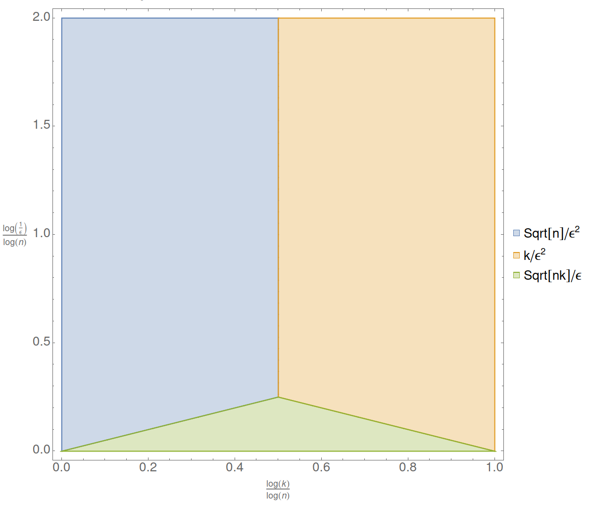
Figure 1: The $x$-axis and $y$-axis represent the quantities $\log(k)/\log(n)$ and $\log(1/\varepsilon)/\log(n)$ respectively. Each point in the graph corresponds to a setting of the parameters $n,k,\varepsilon$, and is colored based on the corresponding dominating term.

The best previous histogram testing algorithm had sample complexity $\widetilde{O}(\sqrt{kn}/\varepsilon^{3})$ [CDGR18], while the best known lower bound was $\widetilde{\Omega}(\sqrt{n}/\varepsilon^{2}+k/\varepsilon)$ [Can16]. We note that the previously best known upper and lower bounds exhibit a polynomial gap, even for constant values of $\varepsilon$ or $k$. For example, in the “large-$k$” regime, where $k=n^{c}$ for some constant $0<c<1$, there was a gap between $\widetilde{O}(n^{1/2+c/2})$ and $\tilde{\Omega}(n^{1/2})$ in the sample complexity. In this regime, Theorem 1 gives the near-optimal bound of $\widetilde{\Theta}(n^{1/2+c/2})$. Similarly, in the “high-accuracy” regime, where $\varepsilon=1/n^{c}$ for some constant $c>0$ (and, say, constant $k$), previous bounds imply that the sample complexity lies between $\widetilde{O}(n^{1/2+3c})$ and $\widetilde{\Omega}(n^{1/2+2c})$, while our result again gives the nearly-tight bound of $\widetilde{\Theta}(n^{1/2+2c})$. These are only two specific examples: more generally, the previously known bounds are suboptimal by polynomial factors in $1/\varepsilon$ when $\varepsilon\geq\sqrt{k/n}$; and by polynomial factors in all parameters $k,n,1/\varepsilon$ when $\varepsilon\leq\sqrt{k/n}$. Theorem 1 settles the sample complexity of the problem, up to logarithmic factors, for every parameter setting.

At a technical level, our sample complexity lower bound construction conceptually differs from previous work in distribution testing, drawing instead from sophisticated techniques from the distribution estimation literature. Our upper bound leverages the “Testing-via-Learning” framework proposed in [ADK15]. The main technical innovation enabling our algorithm is a sample and computationally efficient adaptive algorithm which can simultaneously (1) learn an unknown histogram distribution with unknown interval structure, and (2) identify a domain where the learned result is accurate. We elaborate on these aspects next.

1.3 Overview of Techniques

Sample Complexity Lower Bound.

We begin by discussing our lower bound techniques. We follow the typical high-level approach in proving sample complexity lower bounds in this setting. Namely, we define two ensembles of distributions $D_{\text{YES}}$ and $D_{\text{NO}}$ such that, with high probability, the following conditions are satisfied: (1) a random distribution from $D_{\text{YES}}$ is a $k$-histogram, (2) a random distribution from $D_{\text{NO}}$ is $\varepsilon$-far from any $k$-histogram, and (3) given samples of appropriate size, it is information-theoretically impossible to distinguish a random distribution drawn from $D_{\text{YES}}$ from a random distribution drawn from $D_{\text{NO}}$.

We start by describing our hard instances for the case that the accuracy parameter $\varepsilon$ is a small universal constant. On the one hand, we define $D_{\text{YES}}$ so that all $\mathbf{p}_{i}$’s are the same, except for a “small” number of domain elements, i.e., $c\cdot k$ for a small constant $c\in(0,1)$. On the other hand, for a distribution $\mathbf{p}$ drawn from $D_{\text{NO}}$, $\mathbf{p}_{i}$ will be randomly $0$ or roughly $2/n$, except for at most a constant fraction of the elements. It is not hard to see that, with high probability, a distribution drawn from $D_{\text{YES}}$ (resp. $D_{\text{NO}}$) will be a $k$-histogram (resp. far from being a $k$-histogram).

To ensure that the underlying distributions are indistinguishable using a small sample size, we want to guarantee that for all small values of $t$ the number of elements with exactly $t$ samples will be roughly the same for $D_{\text{YES}}$ and $D_{\text{NO}}$; this property rules out any test statistic relying on counting the number of $t$-way collisions among the samples. Following [Val11, VV13, JVYW15, WY16], this is essentially equivalent to showing that distributions drawn from $D_{\text{YES}}$ and $D_{\text{NO}}$ match their low-degree moments. In particular, for a random pair of distributions $\mathbf{p}$, $\mathbf{p}^{\prime}$ drawn from $D_{\text{YES}}$ and $D_{\text{NO}}$ respectively, we want that $\sum_{i}\mathbf{p}_{i}^{t}$ and $\sum_{i}{\mathbf{p}^{\prime}}^{t}_{i}$ are roughly the same for all small values $t$. We note that the non-exceptional elements of a distribution $\mathbf{p}^{\prime}$ drawn from $D_{\text{NO}}$ — which have probability mass either $0$ or roughly $2/n$ — will have second moment larger than the non-exceptional elements of a distribution $\mathbf{p}$ drawn from $D_{\text{YES}}$ — which have probability mass roughly $1/n$ — by approximately $1/n$. To counteract this discrepancy, the (fewer than $k$) exceptional elements in $D_{\text{YES}}$ must have average mass at least $1/\sqrt{kn}$. Fortunately, using techniques from [VV13, WY19], we are able to construct distributions that match $t=\Theta(\log n)$ moments in which no individual bin has mass more than $\widetilde{O}(1/\sqrt{kn})$. Combining this construction with basic information-theoretic arguments gives us an $\widetilde{\Omega}(\sqrt{kn})$ sample complexity lower bound. We note that this lower bound is tight in the sense that with more than $\widetilde{\Omega}(\sqrt{kn})$ samples one can reliably identify the exceptional elements, as they will each have relatively large numbers of samples with high probability; this allows us to distinguish $D_{\text{YES}}$ from $D_{\text{NO}}$ simply based on the subdistributions over these elements.

Given the aforementioned construction (for constant $\varepsilon$), it is easy to obtain a sample lower bound of $\widetilde{\Omega}(\sqrt{kn}/\varepsilon)$ by mixing our hard instances with the uniform distribution (with mixing weights $\varepsilon$ and $1-\varepsilon$ respectively). In fact, even if the testing algorithm knows in advance which samples come from the uniform part and which samples come from the original hard instance, distinguishing would still require $\widetilde{\Omega}(\sqrt{kn})$ samples from the original hard instance, and therefore $\widetilde{\Omega}(\sqrt{kn}/\varepsilon)$ samples overall. This sample size lower bound turns out to be tight for $\varepsilon$ relatively large, as one can still reliably identify the exceptional bins with only $\widetilde{\Omega}(\sqrt{kn}/\varepsilon)$ samples. However, when $\varepsilon$ becomes sufficiently small, identifying the exceptional bins becomes more challenging. Indeed, if we take $m$ samples, we expect that an exceptional bin has roughly $m\varepsilon/\sqrt{kn}$ more samples than a non-exceptional bin. On the other hand, a non-exceptional bin will have roughly $m/n$ samples with standard deviation $\sqrt{m/n}$. When $m/n\gg m\varepsilon/\sqrt{kn}$ (which happens in the regime $\varepsilon\ll\sqrt{k/n}$), in order for the exceptional bins to be distinguishable, we would need that $m\varepsilon/\sqrt{kn}\gg\sqrt{m/n}$ or $m\gg k/\varepsilon^{2}$ many samples. Using a careful information-theoretic argument, we formalize this intuition to show that $\widetilde{\Omega}(k/\varepsilon^{2})$ is indeed a sample lower bound in this regime.

Sample-Efficient Tester.

The starting point of our efficient tester is the “Testing-via-Learning” approach of [ADK15]. Very roughly speaking, we first design a learning procedure which outputs a distribution $\hat{\mathbf{p}}$ that would be close to $\mathbf{p}$ in $\chi^{2}$ divergence, assuming that $\mathbf{p}$ was in fact a $k$-histogram. Then we use a $\chi^{2}$/$\ell_{1}$ tolerant tester, in the spirit of the one introduced in [ADK15], to distinguish between the cases that $\mathbf{p}$ is close to $\hat{\mathbf{p}}$ in $\chi^{2}$-divergence versus far from $\hat{\mathbf{p}}$ in $\ell_{1}$-distance. We emphasize that the latter step is significantly more challenging than this rough outline suggests, as it is unclear how to perform the first step exactly. Instead, we design a specific learning algorithm with an implicit “hybrid” learning guarantee (see Lemma 5), which in turns requires us to considerably generalize and adapt the “tolerant testing part” to avoid spurious discrepancies (introduced in the imperfect learning stage) which may lead to false negatives.

To implement the first step, we follow the general “learn-and-sieve” idea suggested in [Can16], with important modifications to address the flaw in their approach and its analysis. In particular, suppose that $\mathbf{p}$ is a $k$-histogram. Then, if we knew the corresponding $k$ intervals (that make up the partition for the $k$-histogram), it suffices to learn the mass of $\mathbf{p}$ on each interval, and let $\hat{\mathbf{p}}$ be uniform on each interval (with the appropriate total mass). Of course, a key source of difficulty arises from the fact that we do not know the partition a priori. To circumvent this issue, we divide $[n]$ into (roughly) $K=\Theta(k)$ intervals and try to detect if $\mathbf{p}$ is far in $\chi^{2}$ divergence from being uniform on any of these intervals. If an interval from our partition incurs large $\chi^{2}$ error (we call such an interval bad), we know that $\mathbf{p}$ must not be constant within this interval. Therefore, we proceed to subdivide these bad intervals into roughly equal parts, and recurse on the $\Theta(k)$ intervals in our new partition. Assuming $\mathbf{p}$ is a $k$-histogram, we subdivide at most $k$ intervals in each iteration, since there could be at most $k$ intervals from any interval partition of $[n]$ where $\mathbf{p}$ is not constant. Hence, in each iteration, we decrease the mass of the bad intervals by at least a constant factor. We repeat the process for at most $O(\log(1/\varepsilon))$ many iterations; after this many iterations, the total mass of the bad intervals will become $O(\varepsilon)$, and thus they may be safely ignored.

A significant difference between our method and the approach from [Can16] lies in the method of sieving. In [Can16], it was only said that the algorithm would filter out a subset of breakpoint intervals based on the $\chi^{2}$ statistics (see, e.g., [ADK15]) with the goal of reducing discrepancy; this is where the main gap in their analysis lies, and the particular (flawed) approach they suggested does not seem to be fixable [Can22]. On the contrary, we characterize the exact set of intervals that need to (and can) be removed with a new definition of bad intervals with respect to a given partition $\mathcal{I}$ of $[n]$ (see Definition 2). Based on that, our approach is to search for any subintervals $J$ (not necessarily an interval in $\mathcal{I}$) on which the $\chi^{2}$ divergence between $\mathbf{p}$ and $\hat{\mathbf{p}}$ — an approximation of $\mathbf{p}$ assuming $\mathbf{p}$ is uniform over intervals within the given partition — is more than $\widetilde{\Omega}(\varepsilon^{2}/k)$. For an interval $I$ from the partition $\mathcal{I}$, we show the inclusion of such a “bad subinterval” $J\subseteq I$ then certifies the “badness” of $I$ itself. To find such a $J$, we need a technique for accurately approximating $\mathbf{p}(J)$ simultaneously for all intervals $J\subseteq[n]$, in both absolute and relative error. We note that this is a notion of approximation much stronger than what classical tools from empirical process theory, such as the VC inequality (see, e.g., [DL01]), provide. Notice that for a fixed interval $J\subseteq[n]$, taking the empirical distribution over $b$ samples gives an estimate $\mathbf{q}$ of $\mathbf{p}$ such that $\left|\mathbf{q}(J)-\mathbf{p}(J)\right|<\sqrt{\mathbf{p}(J)/b}$ with constant probability. By taking $\Theta(\log(n))$ batches of samples (each containing $b$ i.i.d. samples from $\mathbf{p}$), and computing the median value of all of the $\mathbf{q}(J)$’s, with high probability for each $J$, we then obtain an estimate $\hat{\varphi}(J)$  for which the above condition holds. Using this subroutine, as long as $b$ is at least $\Omega(k/\varepsilon^{2})$, we can ensure that $|\hat{\varphi}(J)-\mathbf{p}(J)|^{2}/\mathbf{p}(J)\ll\varepsilon^{2}/k$, and we can then safely use our estimate $\hat{\varphi}(J)$ as a proxy for $\mathbf{p}(J)$ for the detection of those “bad subintervals” for which $|\mathbf{p}(J)-\hat{\mathbf{p}}(J)|^{2}/\hat{\mathbf{p}}(J)$ is large, which in turns certify the bad intervals from a given partition. This suffices unless $\mathbf{p}(J)$ is substantially larger than our estimate $\hat{\mathbf{p}}(J)$.

Unfortunately, the ratio between $|\hat{\varphi}(J)-\mathbf{p}(J)|^{2}/\hat{\mathbf{p}}(J)$ and $|\hat{\varphi}(J)-\mathbf{p}(J)|^{2}/\mathbf{p}(J)$ (in particular $\mathbf{p}(J)/\hat{\mathbf{p}}(J)$) can be unbounded when $\mathbf{p}(J)$ is smaller than $1/b$. In such a case, in a collection of $b$ samples from $\mathbf{p}$, we are likely to see no samples in $J$, and thus our empirical estimate $\hat{\mathbf{p}}(J)$ will be $0$. We can fix this issue (i.e., the case where $\hat{\mathbf{p}}(J)$ is actually $0$) by mixing both $\mathbf{p}$ and $\hat{\mathbf{p}}$ with the uniform distribution, thus allowing us to assume that $\hat{\mathbf{p}}(J)\geq|J|/2n\geq 1/(2n)$. Yet, this still leaves a potential gap of roughly $n/b$ between the ratio of $\mathbf{p}(J)$ and $\hat{\mathbf{p}}(J)$. Fortunately, if we select $b\gg\sqrt{nk}/\varepsilon$, we will have that $|\hat{\varphi}(J)-\mathbf{p}(J)|^{2}/\mathbf{p}(J)\ll\varepsilon/\sqrt{nk}$, and even accounting for losing a factor of $b/n$, we will still have that $|\hat{\varphi}(J)-\mathbf{p}(J)|^{2}/\mathbf{p}(J)\ll\varepsilon^{2}/k$. This implies that we will successfully detect any bad intervals and achieve our learning guarantees.

1.4 Prior and Related Work

The field of distribution property testing [BFRSW00] has been extensively investigated in the past couple of decades, see [Rub12, Gol17, Can20] for two recent surveys and a book on the topic. A large body of the literature has focused on characterizing the sample size needed to test properties of arbitrary discrete distributions of a given support size. This regime is fairly well understood for many properties of interest, and in particular for symmetric properties (i.e., invariant under permutation of the domain). For a range of such properties, there exist sample-optimal testers [Pan08a, CDVV14, DKN15a, ADK15, DK16, DGPP16, CDS18, Gol17, DGPP18, CDKS18]. We note that the property of being a histogram is not symmetric.

Motivated by the question of building provably good succinct representations of a dataset from only a small subsample of the data, [ILR12] first introduced histogram testing as a preliminary, ultra-efficient decision subroutine to find the best parameter $k$ for the number of bins. They provided an algorithm for this task which required $\widetilde{O}(\sqrt{kn}/\varepsilon^{5})$ samples from the dataset, a sample complexity which beats the naïve approach (reading and processing the whole dataset) for small values of $k$ and relatively large values of the accuracy parameter $\varepsilon$. Subsequent work [CDGR18] reduced the dependence on $\varepsilon$ from quintic to cubic, giving an algorithm with sample complexity $\widetilde{O}(\sqrt{kn}/\varepsilon^{3})$. This bound was, however, still quite far from the “trivial” lower bound of $\Omega(\sqrt{n}/\varepsilon^{2})$, which follows from a reduction to uniformity testing (i.e., the case $k=1$) [Pan08].

Prior to the current work, an $\widetilde{\Omega}(\sqrt{n}/\varepsilon^{2}+k/\varepsilon)$ sample complexity lower bound was obtained in [Can16]. The latter work also claimed a testing algorithm with sample complexity $\widetilde{O}(\sqrt{n}/\varepsilon^{2}+k/\varepsilon^{3})$. Unfortunately, as pointed out in [Can22], the algorithm proposed in [Can16] is incorrect due to a technical flaw in the analysis. This leaves the sample complexity of the problem open for even constant $\varepsilon$. The lower bound of [Can16] is valid and relies on a reduction of histogram testing to the well-studied problem of support size estimation. Consequently, it provably cannot be improved to provide either (i) a quadratic dependence on $\varepsilon$, i.e., $\widetilde{\Omega}(k/\varepsilon^{2})$, or (ii) coupling between the two domain parameters $k,n$, i.e., $\widetilde{\Omega}(\sqrt{nk}/\varepsilon)$. Our work resolves the complexity of histogram testing, for the entire parameter range, within logarithmic factors.

Finally, we note that a number of works have obtained algorithms and lower bounds for related, yet significantly different, testing problems. Specifically, [DK16] gave a sample-optimal testing algorithm for the special case of our problem where the $k$ intervals are known a priori. This special case turns out to be significantly simpler. Moreover, a number of works [DKN15a, DKN15, DKN17] have obtained identity and equivalence testers under the assumption that the input distributions are $k$-histograms.

1.5 Preliminaries

We denote by $\operatorname{TV}\left(\mathbf{p},\mathbf{q}\right)$ the total variation (TV) distance between probability distributions $\mathbf{p},\mathbf{q}$ over $[n]\coloneqq\{1,2,\dots,n\}$, defined as

$$\operatorname{TV}\left(\mathbf{p},\mathbf{q}\right)\coloneqq\sup_{S\subseteq[n]}(\mathbf{p}(S)-\mathbf{q}(S))=\frac{1}{2}\sum_{i=1}^{n}|\mathbf{p}(i)-\mathbf{q}(i)|,$$

where $\mathbf{p}(S)\coloneqq\sum_{i\in S}\mathbf{p}(i)$. We will make essential use of the $\chi^{2}$-divergence of $\mathbf{p}$ with respect to $\mathbf{q}$, defined as

$$d_{\chi^{2}}\left(\mathbf{p}\big{\|}\mathbf{q}\right)\coloneqq\sum_{i=1}^{n}\frac{\left(\mathbf{p}_{i}-\mathbf{q}_{i}\right)^{2}}{\mathbf{q}_{i}}.$$

We will also require generalizations of these definitions on restrictions of the domain. In particular, given $S\subseteq[n]$, we use the notation $\operatorname{TV}^{S}\left(\mathbf{p},\mathbf{q}\right)\coloneqq(1/2)\sum_{i\in S}|\mathbf{p}(i)-\mathbf{q}(i)|$ and $d_{\chi^{2}}^{S}\left(\mathbf{p}\big{\|}\mathbf{q}\right)\coloneqq\sum_{i\in S}\left(\mathbf{p}_{i}-\mathbf{q}_{i}\right)^{2}/\mathbf{q}_{i}$. We note that for any $S\subseteq[n]$, it holds that $\text{TV}^{S}(\mathbf{p},\mathbf{q})^{2}\leq\frac{1}{4}d_{\chi^{2}}^{S}\left(\mathbf{p}\big{\|}\mathbf{q}\right)$.

The asymptotic notation $\tilde{O}$ (resp. $\tilde{\Omega}$) suppresses logarithmic factors in its argument, i.e., $\tilde{O}(f(n))=O(f(n)\log^{c}f(n))$ and $\tilde{\Omega}(f(n))=\Omega(f(n)/\log^{c}f(n))$, where $c>0$ is a universal constant. The notations $\ll$ and $\gg$ intuitively mean “much less than” and “much greater than” respectively. Formally, we write $f(n)\ll g(n)$ to denote that $f(n)<c\cdot g(n)$, for some universal constant $c>0$.

2 Main Algorithmic Result: Near-Optimal Histogram Tester

A preliminary simplification.

Without loss of generality, we will assume that $\mathbf{p}(i)\geq\frac{1}{2n}$ for every $i\in[n]$. Indeed, this can be ensured by mixing the unknown distribution with the uniform distribution $\mathbf{u}_{n}$ on $[n]$ beforehand, i.e., $\mathbf{p}^{\prime}\coloneqq\frac{1}{2}(\mathbf{p}+\mathbf{u}_{n})$ (see Fact 6 in Appendix for how to sample from $\mathbf{p}^{\prime}$ efficiently). It is easy to see that $\mathbf{p}^{\prime}$ remains a histogram after mixing: $\mathbf{p}^{\prime}\in\mathcal{H}_{k}^{n}$ if $\mathbf{p}\in\mathcal{H}_{k}^{n}$, and $\mathbf{p}^{\prime}$ is at least $(\varepsilon/2)$-far away from every histogram if $\mathbf{p}$ is $\varepsilon$-far from every histogram.

Testing via Learning.

The high-level approach is to leverage the Testing-via-Learning framework proposed in [ADK15]. In particular, suppose we have a learning algorithm capable of constructing a hypothesis $\hat{\mathbf{p}}$ that is close to $\mathbf{p}$ in $\chi^{2}$ divergence when $\mathbf{p}\in\mathcal{H}_{n}^{k}$. Then, (1) if $\mathbf{p}\in\mathcal{H}_{k}^{n}$, we will have that $\mathbf{p}$ and $\hat{\mathbf{p}}$ are close and (as a consequence of this) that $\hat{\mathbf{p}}$ is close to being a $k$-histogram. Yet, (2) if $\mathbf{p}$ is far from being a $k$-histogram, then by the triangle inequality we must have either that $\hat{\mathbf{p}}$ is far from being a $k$-histogram, or that $\mathbf{p}$ and $\hat{\mathbf{p}}$ are far from each other in $\ell_{1}$ distance. We can use dynamic programming to efficiently check the explicit description is indeed close to a $k$-histogram in $\ell_{1}$ distance (see Lemma 4.11 of [CDGR18]). To verify that $\mathbf{p}$ and $\hat{\mathbf{p}}$ are close, we will use a result of [ADK15] on tolerant identity testing. In particular, given an explicit description $\hat{\mathbf{p}}$, the tester takes samples from the unknown distribution $\mathbf{p}$ and decides whether $\mathbf{p}$ and $\hat{\mathbf{p}}$ are closed in $\chi^{2}$ divergence or far in $\ell_{1}$ distance. We remark that $\hat{\mathbf{p}}$ can be relaxed to be a positive measure.

Lemma 1 (Adapted from Lemmas 2 and 3 [ADK15]).

Let $\mathbf{p}$ and $\hat{\mathbf{p}}$ be a distribution and a positive measure defined on $[n]$ respectively. Fix $\varepsilon\in(0,1)$ and let $\mathcal{A}=\{i\in[n]:\hat{\mathbf{p}}(i)\geq\varepsilon/(50n)\}$. There exists a tester Tolerant-Identity-Test, which takes $\operatorname{Poi}(m)$ i.i.d. samples from $\mathbf{p}$ and outputs Accept if $d_{\chi^{2}}^{\mathcal{A}}\left(\mathbf{p}\big{\|}\hat{\mathbf{p}}\right)\leq\varepsilon^{2}/500$ and Reject if $\text{TV}^{\mathcal{A}}\left(\mathbf{p},\hat{\mathbf{p}}\right)\geq\varepsilon$ with constant probability.

Outline for Learning.

If $\mathbf{p}\in\mathcal{H}_{k}^{n}$ and we know the partition of $\mathbf{p}$ in advance, one can learn $\mathbf{p}$ up to error $\varepsilon^{2}$ in $\chi^{2}$ divergence with $\Theta(k/\varepsilon^{2})$ samples (following the analysis of Laplace estimator from [KOPS15]). Without the partition information, we can nonetheless achieve a weaker guarantee. That is, we can output a fully specified measure $\hat{\mathbf{p}}$ on $[n]$, together with a subset of the domain, $\mathcal{G}\subseteq[n]$, such that $d_{\chi^{2}}^{\mathcal{G}}\left(\mathbf{p}\big{\|}\hat{\mathbf{p}}\right)$ is small. In particular, we can achieve the guarantee in three steps.

1. Equally divide the domain $[n]$ into $K\gg k$ many intervals (Lemma 2).

2. Output a succinct measure $\hat{\mathbf{p}}$ that is constant on each interval specified by Step (i) (Section 2.1).

3. Identify the intervals $\mathcal{B}$ where $d_{\chi^{2}}^{\mathcal{B}}\left(\mathbf{p}\big{\|}\hat{\mathbf{p}}\right)$ is large (Section 2.2) and take $\mathcal{G}=[n]\backslash\mathcal{B}$.

The fact that we only have $\mathbf{p}$ and $\hat{\mathbf{p}}$ close in $\chi^{2}$ divergence on a subdomain $\mathcal{G}$ is a reasonable compromise, as long as $\mathbf{p}(\mathcal{B}),\hat{\mathbf{p}}(\mathcal{B})\ll\varepsilon$: if $\mathbf{p}$ is $\varepsilon$-far away from $\hat{\mathbf{p}}$ in $\ell_{1}$ distance on $[n]$, $\mathbf{p}$ is at least $(\varepsilon-\mathbf{p}(\mathcal{B})-\hat{\mathbf{p}}(\mathcal{B}))$-far away from $\hat{\mathbf{p}}$ on $[n]\backslash\mathcal{B}$. Otherwise, we may take more samples from $\mathbf{p}$ restricted to $\mathcal{B}$ and subdivide the problematic intervals identified in Step (iii). Repeating the above steps iteratively then brings us to the case $\mathbf{p}(\mathcal{B})\ll\varepsilon$.

Equitable Partition.

The first step is to divide the domain into $\Theta(k)$ many intervals over which the masses of $\mathbf{p}$ are approximately equal. As shown in [ADK15], this can be done with $\widetilde{\Theta}(k)$ many samples through a routine we denote by Approx-Divide. We also need a routine for subdividing a set of disjoint intervals into even lighter subintervals. Nonetheless, one can reduce the subdividing task to domain partitioning by running Approx-Divide on the subdistribution restricted to the set of disjoint intervals. For clarity of exposition, the proofs for this refinement of the subroutine from [ADK15] are provided in Appendix A.1.

Lemma 2.

There exists an algorithm Approx-Sub-Divide that, given parameters $\delta\in(0,1]$ and integer $B>1$, as well as a set of disjoint intervals $\mathcal{I}=\{I_{1},I_{2},\cdots,I_{q}\}$, given sample access to $\mathbf{p}$ on $[n]$, outputs a list of partitions $\mathcal{S}_{1},\dots,\mathcal{S}_{q}$, where $\mathcal{S}_{i}$ is the partition of the interval $I_{i}\in\mathcal{I}$, such that the following holds with probability at least $1-\delta$.

1. The algorithm uses $O\left(B/\mathbf{p}(\mathcal{I})\cdot\log\big{(}B/\delta\big{)}\right)$ samples.

2. The output contains at most $(8B+q)$ intervals in total.

3. Every non-singleton interval $S\in\bigcup_{j=1}^{q}\mathcal{S}_{j}$ satisfies $\mathbf{p}(S)\leq\mathbf{p}(\mathcal{I})\cdot 16/B$.

2.1 Simultaneously Estimating Mass of Intervals

In this section, we first introduce Interval-Mass-Estimate, a subroutine that can accurately approximate the mass of $\mathbf{p}(J)$ for all intervals $J\subseteq[n]$ simultaneously, and then show how we can use it to learn $\mathbf{p}$ (assuming $\mathbf{p}\in\mathcal{H}_{n}^{k}$).

Interval-Mass-Estimate first divides the number of samples drawn into $\Theta(\log(n/\delta))$ batches. For an interval $I$, we compute the estimate (number of samples falling in $I$ divided by the batch size) for each batch separately and compute the median over the statistics. This is often referred as the “Median Trick” and is crucial in achieving the learning guarantees with high probability.

Lemma 3.

Let be $\mathbf{p}$ be supported on $[n]$ such that $\mathbf{p}(i)\geq 1/(2n)$. Fix $b\in\mathbb{Z}^{+}$ and $\delta\in(0,1]$. The algorithm Interval-Mass-Estimate takes $6b\log(n/\delta)$ i.i.d. samples from $\mathbf{p}$ and outputs $\hat{\varphi}$, a map from sub-intervals of $[n]$ to real values, such that, with probability at least $1-\delta$, for every sub-interval $I\subseteq[n]$ it holds that ${\mathbf{p}(I)}/{\hat{\varphi}(I)}\leq\max(2\,,8n/b)$, ${\hat{\varphi}(I)}/{\mathbf{p}(I)}\leq 3$ and $\left|\hat{\varphi}(I)-\mathbf{p}(I)\right|\leq\sqrt{\mathbf{p}(I)/b}$.

Proof of Lemma 3.

We provide below the pseudocode of the algorithm, before analyzing its guarantees.

Algorithm 1 Interval-Mass-Estimate

1:$m$ i.i.d. samples from distribution $\mathbf{p}$ on $[n]$; failure probability $\delta$.

2:Let $T\coloneqq 6\log(n/\delta)$.

3:Split the samples into $T$ batches $S^{(1)},S^{(2)},\cdots,S^{(T)}$, each of $b\coloneqq m/T$ samples.

4:Initialize a Map $\hat{\varphi}\colon\mathcal{I}\mapsto\mathbb{R}$ which maps sub-intervals of $[n]$ to real values.

5:for all intervals $I\subseteq[n]$ do

6:     Let $X_{j}^{(i)}$ be the number of samples falling in interval $I_{j}$ from samples $S^{(i)}$.

7:     Compute the median $X_{j}\coloneqq\operatorname{median}_{1\leq i\leq T}\big{(}X_{j}^{(i)}\big{)}$. Accordingly, set

$$\hat{\varphi}(I)\coloneqq\max\!\left(\frac{X_{j}}{b},\frac{\left|I\right|}{2n}\right).$$

8:Output the map $\hat{\varphi}$.

The following claim about the “Median Trick” will be useful.

Claim 2.

Let $I$ be an interval (or subset) over $[n]$ and $\mathbf{p}$ a distribution over $[n]$. For $\delta\in(0,1)$, assume one takes $T\coloneqq 3\log(1/\delta)$ batches of i.i.d. samples from $\mathbf{p}$ where each batch is of size $b\in\mathbb{Z}^{+}$. Denote by $X_{I}^{(i)}$ the number of samples falling in $I$ from the $i$-th batch, for $1\leq i\leq T$. Then, the median $X_{I}\coloneqq\operatorname{median}_{i}(X_{I}^{(i)})$ satisfies

$$\left|\frac{X_{I}}{b}-\mathbf{p}(I)\right|\leq 3\sqrt{\frac{\mathbf{p}(I)}{b}}\quad\text{ and }\quad\frac{X_{I}}{b}\leq 3\mathbf{p}(I)\,,$$

with probability at least $1-\delta$.

Proof.

For $X_{I}^{(1)}$, it follows from standard application of Chernoff Bound and Markov’s Inequality that

$$\left|\frac{X_{I}}{b}-\mathbf{p}(I)\right|\leq 3\sqrt{\frac{\mathbf{p}(I)}{b}}$$ (1)

$$\frac{X_{I}}{b}\leq 3\mathbf{p}(I)$$ (2)

each individually with probability at least $2/3$. Let $a_{i}$ be the indicator variable such that Equation (1) holds for $X_{I}^{(i)}$ for $1\leq i\leq T$. If more than half of $a_{i}$s are true, then it follows the median $X_{I}$ will also satisfy Equation (1). Since $a_{i}$s are independent, this happens with probability precisely $Y>T/2$, where $Y\sim Bin(T,2/3)$. By the multiplicative Chernoff’s Bound, the failure probability is bounded above by

$$\Pr\left(Y\leq\frac{1}{2}T\right)=\Pr\left(Y\leq(1-\frac{1}{4})\cdot\frac{2}{3}\cdot T\right)\leq\left(\frac{\exp(-1/4)}{(3/4)^{3/4}}\right)^{2/3\cdot T}\,.$$

Note that we indeed have $\left(\frac{\exp(-1/4)}{(3/4)^{3/4}}\right)^{2/3\cdot T}\leq\delta/2$ given $T\geq 3\log(1/\delta)$. A similar argument holds for Equation (2) and the claim follows by applying the union bound. ∎

With this in hand, we are ready to establish Lemma 3. Let $I\subseteq[n]$ be an arbitrary interval and $X_{I}$ be the median of the numbers of samples falling in from each batch. By Claim 2, we have that

$$\left|\frac{X_{I}}{b}-\mathbf{p}(I)\right|\leq\sqrt{\mathbf{p}(I)/b}\,,$$ (3)

$$\frac{X_{I}}{b}\leq 3\mathbf{p}(I)$$ (4)

with probability at least $1-\delta/(2n^{2})$. Since $\mathbf{p}(i)>1/(2n)$ for any $i\in[n]$, the max operation decreases the distance between $\mathbf{p}$ and $\hat{\mathbf{p}}$ pointwise. Hence, with probability at least $1-\delta/(2n^{2})$, we have

$$\left|\hat{\varphi}(I)-\mathbf{p}(I)\right|\leq\sqrt{\mathbf{p}(I)/b}\,.$$ (5)

Since there are at most $n^{2}$ intervals $I\subseteq[n]$ overall, by a union bound over all of them, we have that Equation 5 holds simultaneously with probability at least $1-\delta/2$ for every interval $I$.

To show that the ratio $\mathbf{p}(I)/\hat{\varphi}(I)$ is bounded, we first consider the case $\mathbf{p}(I)\leq 4/b$. Since $\hat{\varphi}(I)>{1}/{(2n)}$, it is easy to see that $\mathbf{p}(I)/\hat{\varphi}(I)\leq 8n/b$. Otherwise, we have $\mathbf{p}(I)>4/b$. Following Equation 5, it holds that

$$\left|\mathbf{p}(I)-\hat{\varphi}(I)\right|\leq\sqrt{\mathbf{p}(I)/b}\leq\frac{1}{2}\mathbf{p}(I)\,,$$

This then implies that

$$\frac{\mathbf{p}(I)}{\hat{\varphi}(I)}\leq 2\,.$$

Lastly, since $\mathbf{p}(I)\geq\left|I\right|/(2n)$, together with Equation 4, we have

$$\frac{\hat{\varphi}(I)}{\mathbf{p}(I)}=\frac{\max\left(\left|I\right|/(2n),X_{I}/b\right)}{\mathbf{p}(I)}\leq 3.$$

This concludes the proof. ∎

Let $\mathcal{I}$ be a partition of $[n]$. We try to learn $\mathbf{p}$ pretending that $\mathbf{p}$ is constant over each interval within $\mathcal{I}$ with the routine Empirical-Learning. In particular, the algorithm uses Interval-Mass-Estimate to obtain estimations of the mass of $I\in\mathcal{I}$ and then flattens the mass uniformly among elements $i\in I$. Notice that, due to the application of the median trick, the output is not necessarily a distribution but rather a positive measure $\hat{\mathbf{p}}$ on $[n]$ which is constant over each interval within $\mathcal{I}$.

If $\mathbf{p}$ is indeed a $k$-histogram, errors are only incurred on a special type of intervals (of which there are at most $k$), which we refer to as the breakpoint intervals.

Definition 1 (Breakpoint Intervals).

Given a $k$-histogram $\mathbf{p}$ on $[n]$, we say that $i\in[n]$ is a breakpoint with respect to $\mathbf{p}$ if $\mathbf{p}(i)\neq\mathbf{p}(i+1)$; and that an interval $I\subseteq[n]$ is a breakpoint interval (with respect to $\mathbf{p}$) if $I$ contains at least one breakpoint.

With Definition 1 in mind, we now specify the formal learning guarantees.

Lemma 4.

Suppose $\mathbf{p}\in\mathcal{H}_{k}^{n}$. Let $\mathcal{I}$ be a partition of $[n]$ into $K$ intervals. Let $b\in\mathbb{Z}^{+}$, $\delta\in(0,1]$ and $T\coloneqq 6\log(K/\delta)$. There exists an algorithm Empirical-Learning that, given $m\coloneqq Tb$ i.i.d. samples from $\mathbf{p}$, outputs a positive measure $\hat{\mathbf{p}}$ which satisfies the following with probability at least $1-\delta$. (i) $\hat{\mathbf{p}}$ is constant within each interval in $\mathcal{I}$. (ii) For every sub-intervals $J\subseteq I$ where $I\in\mathcal{I}$, is a non-breakpoint interval with respect to $\mathbf{p}$, we have ${\mathbf{p}(J)}/{\hat{\mathbf{p}}(J)}\leq\max(2,8n/b)$ and $\left|\hat{\mathbf{p}}(J)-\mathbf{p}(J)\right|\leq\sqrt{\mathbf{p}(J)/b}$.

Proof of Lemma 4.

The pseudocode of the algorithm is provided below.

Algorithm 2 Empirical-Learning

1:$m$ i.i.d. samples from distribution $\mathbf{p}$ on [n]; partition $\mathcal{I}=\{I_{1},I_{2},\cdots,I_{K}\}$ of the domain $[n]$; failure probability $\delta$.

2:Let $\mathcal{S}$ denote the multiset of the $m$ i.i.d. samples.

3:Construct the Interval Estimator $\hat{\varphi}\leftarrow\textup{\sc{}Interval-Mass-Estimate}(\mathcal{S},\delta).$

4:for $1\leq j\leq K$ do

5:     Compute the estimate $\hat{\mathbf{p}}(i)\coloneqq\frac{\hat{\varphi}(I_{j})}{\left|I_{j}\right|}\qquad 1\leq j\leq K,i\in I_{j}\;.$

6:Output the measure $\hat{\mathbf{p}}$.

Let $I$ be a non-breakpoint interval. It is easy to see that $\hat{\mathbf{p}}(I)=\hat{\varphi}(I)$. By Lemma 3, it holds that

$$\frac{\mathbf{p}(I)}{\hat{\mathbf{p}}(I)}\leq\max(2,8n/b)\,,$$

$$\left|\hat{\mathbf{p}}(I)-\mathbf{p}(I)\right|\leq\sqrt{\mathbf{p}(I)/b}\,.$$

with probability at least $1-\delta$. Conditioned on that, we easily have, for any sub-interval $J\subseteq I$,

$$\frac{\mathbf{p}(J)}{\hat{\mathbf{p}}(J)}=\frac{\mathbf{p}(I)}{\hat{\mathbf{p}}(I)}\leq\max(2,8n/b)\;,$$

since both $\mathbf{p}$ and $\hat{\mathbf{p}}$ are uniform within $I$. Furthermore, we also have

$$\left|\mathbf{p}(J)-\hat{\mathbf{p}}(J)\right|=\left|\mathbf{p}(I)-\hat{\mathbf{p}}(I)\right|\cdot\frac{|J|}{|I|}\leq\sqrt{\frac{\mathbf{p}(I)}{b}}\cdot\frac{|J|}{|I|}=\sqrt{\frac{\mathbf{p}(J)}{b}}\cdot\sqrt{\frac{|J|}{|I|}}\leq\sqrt{\frac{\mathbf{p}(J)}{b}}\,,$$

where the first equality follows from the fact that $\mathbf{p}$ and $\hat{\mathbf{p}}$ are both uniform within $I$, the second inequality follows from our conditioning, and the last inequality follows from $|J|\leq|I|$. ∎

By combining the two guarantees in (ii) in Lemma 4, one can see the $\chi^{2}$ divergence between $\mathbf{p}$ and $\hat{\mathbf{p}}$, restricted to the non-breakpoint intervals, will be at most $\varepsilon^{2}$ with high probability if taking $\Theta(KT/\varepsilon^{2})$ many samples. Following a result from [KOPS15, Can16], one only needs $\Theta(K/\varepsilon^{2})$ samples to learn a $K$-histogram up to $\varepsilon^{2}$ error in this restricted notion of $\chi^{2}$ divergence. One may wonder whether this is enough for us, and if the stronger (but less natural) guarantees provided by Lemma 4, which end up increasing the number of samples required, are necessary. As we will see in the next section, we indeed need not only that the $\chi^{2}$ divergence is small, but also that the ratio $\mathbf{p}(I)/\hat{\mathbf{p}}(I)$ is bounded for all non-breakpoint intervals. In particular, this latter property enables us to compute relatively accurate estimates of the $\chi^{2}$ divergence restricted to subintervals and (consequently) to tell whether $\mathbf{p}$ is constant or from far from being constant on an interval.

2.2 Bad Interval Detection

While large contributions to the $\chi^{2}$ divergence (assuming the learning phase was successful) will only come from breakpoint intervals, not all of them will necessarily contribute significantly to the $\chi^{2}$ divergence. In particular, a breakpoint interval is only considered “bad”, and needs to be filtered out, if the error incurred is proportional to the number of breakpoints within.

We now give the formal definition of such a “bad interval.”

Definition 2 ($\varepsilon$-Bad-Interval).

Fix a partition $\mathcal{I}$ of $[n]$ containing $K$ intervals. Let $I\in\mathcal{I}$ be a breakpoint interval of $\mathbf{p}$. Furthermore, suppose $I$ contains $j-1$ breakpoints, i.e., $\mathbf{p}$ is $j$-piecewise uniform in $I$. We say that $I\in\mathcal{I}$ is an $\varepsilon$-bad interval with respect to $\hat{\mathbf{p}}$ and $\mathcal{I}$ if $d_{\chi^{2}}^{I}\left(\mathbf{p}\big{\|}\hat{\mathbf{p}}\right)\geq j\cdot\varepsilon^{2}/K$.

The definition suits our purpose for two reasons. (i) The total $\chi^{2}$ error between $\mathbf{p}$ and $\hat{\mathbf{p}}$ on the set of “good” intervals (complement of the set of “bad” intervals) is small. Indeed, let $\mathcal{G}\in\mathcal{I}$ be a set containing no $\varepsilon$-bad intervals. Since there are at most $K$ intervals contained in $\mathcal{G}$ and $k$ breakpoints contained in the intervals in $\mathcal{G}$, it is easy to see that $d_{\chi^{2}}^{\mathcal{G}}\left(\mathbf{p}\big{\|}\hat{\mathbf{p}}\right)\leq O(\varepsilon^{2})$. (ii) One can reliably separate bad intervals from non-breakpoint intervals assuming the learning phase was successful. To see why, note that in that case every non-breakpoint interval $I$ satisfies $d_{\chi^{2}}^{J}\left(\mathbf{p}\big{\|}\hat{\mathbf{p}}\right)\ll\varepsilon^{2}/K$ for all $J\subseteq I$ with high probability. On the contrary, for any bad interval $I$, we claim there must be a sub-interval $Q\subseteq I$ where $d_{\chi^{2}}^{Q}\left(\mathbf{p}\big{\|}\hat{\mathbf{p}}\right)\geq\varepsilon^{2}/K$ and both $\mathbf{p}$ and $\hat{\mathbf{p}}$ are constant within. In particular, if $I$ is an $\varepsilon$-bad interval that contains $(j-1)$ breakpoints, we then have a partition $\{Q_{1},\cdots,Q_{j}\}$ of $I$ over which $\mathbf{p}$ is piecewise constant and at least one of them will have $\chi^{2}$ error at least $\varepsilon^{2}/K$.

Our next step is to show how we can leverage the separating condition to design an efficient bad interval detection mechanism. This is where our method significantly differs from [Can16]. At a high level, we take another set of independent samples to get an estimate $\hat{\varphi}(Q)$ of $\mathbf{p}(Q)$ for all $Q\subseteq[n]$ simultaneously. Then, we compare $\hat{\varphi}(Q)$ with $\hat{\mathbf{p}}(Q)$ to see whether we have $d_{\chi^{2}}^{Q}\left(\mathbf{p}\big{\|}\hat{\mathbf{p}}\right)\geq\varepsilon^{2}/K$, which would in turn imply the interval $I\supseteq Q$ from the given partition is $\varepsilon$-bad. We next provide the pseudo-code for Learn-and-Sieve, which finds a positive measure $\hat{\mathbf{p}}$ on $[n]$ and a domain $\mathcal{B}$ such that $d_{\chi^{2}}^{[n]\backslash\mathcal{B}}\left(\mathbf{p}\big{\|}\hat{\mathbf{p}}\right)\leq O(\varepsilon^{2})$ provided $\mathbf{p}\in\mathcal{H}_{k}^{n}$. For the sake of exposition, we defer its detailed analysis to Appendix A.2, and provide here an outline of the argument.

Algorithm 3 Learn-And-Sieve

1:Sample access to $\mathbf{p}$; a partition $\mathcal{I}$ of $[n]$ containing $K$ intervals; accuracy $\varepsilon$; failure probability $\delta$.

2:Let $m=C\cdot(K/\varepsilon^{2}+\sqrt{Kn}/\varepsilon)\cdot\log(n/\delta)$ for a sufficiently large constant $C$.

3:Draw $2m$ i.i.d. samples from $\mathbf{p}$ and split the samples evenly into $\mathcal{S}_{1},\mathcal{S}_{2}$.

4:$\hat{\mathbf{p}}\leftarrow\textup{\sc{}Empirical-Learning}\left(\mathcal{S}_{1},\mathcal{I},\delta/4\right)$, $\hat{\varphi}\leftarrow\textup{\sc{}Interval-Mass-Estimate}(\mathcal{S}_{2},\delta/4)$, $\mathcal{B}\leftarrow\{\}$.

5:for all intervals $Q\subseteq I$ for some $I\in\mathcal{I}$ do

6:     if  $\hat{\varphi}(Q)/{\hat{\mathbf{p}}(Q)}>6\cdot\max(1,\varepsilon\sqrt{n/K})$ or $\left|\hat{\varphi}(Q)-\hat{\mathbf{p}}(Q)\right|>\frac{1}{2}\sqrt{\hat{\mathbf{p}}(Q)\varepsilon^{2}/K}$ then

7:         Add $I$ to $\mathcal{B}$.      

8:Output Reject if $\mathcal{B}$ contains more than $k$ intervals. Otherwise, return $\mathcal{B}$, $\hat{\mathbf{p}}$.

Lemma 5 (Sieving Lemma).

Given a partition $\mathcal{I}$ containing $K$ intervals, sample access to $\mathbf{p}$ on $[n]$ and $\delta\in(0,1)$. Then, the output of Learn-and-Sieve (Algorithm 3) satisfies the following. (i) Suppose $\mathbf{p}\in\mathcal{H}_{k}^{n}$. Then the algorithm returns a positive measure $\hat{\mathbf{p}}$ and $\mathcal{B}$ such that $d_{\chi^{2}}^{[n]\backslash\mathcal{B}}\left(\mathbf{p}\big{\|}\hat{\mathbf{p}}\right)\leq\varepsilon^{2}$ with probability at least $1-\delta$. (ii) The output $\mathcal{B}$ contains at most $k$ intervals (if the algorithm does not reject). (iii) At most $O(({K}/{\varepsilon^{2}}+{\sqrt{Kn}}/{\varepsilon})\cdot\log(n/\delta))$ samples are used.

Proof Sketch.

We claim that if $\mathbf{p}\in\mathcal{H}_{k}^{n}$, then $\mathcal{B}$ contains all the $\varepsilon$-bad intervals and no non-breakpoint intervals with high probability. Let $I$ be a non-breakpoint interval. For $b=\Theta(m/\log(n/\delta))=\Theta(K/\varepsilon^{2}+\sqrt{Kn}/\varepsilon)$, with high probability we have that $\left|\hat{\varphi}(Q)-\mathbf{p}(Q)\right|\leq\sqrt{\mathbf{p}(Q)/b}$, $\left|\hat{\mathbf{p}}(Q)-\mathbf{p}(Q)\right|\leq\sqrt{\mathbf{p}(Q)/b}$ and ${\mathbf{p}(Q)}/{\hat{\mathbf{p}}(Q)}\leq\max(2\,,8\cdot n/b)$, which follow from Lemmas 3 and 4. Combining this with the triangle inequality and our choice of $b$ implies the second condition of Line 6 will be false. The first condition can be shown to be false by rewriting $\hat{\varphi}(Q)/\hat{\mathbf{p}}(Q)$ as ${\hat{\varphi}(Q)}/{\mathbf{p}(Q)}\cdot{\mathbf{p}(Q)}/{\hat{\mathbf{p}}(Q)}$, which are themselves bounded, with high probability, by $3$ and $\Theta(1)\cdot\max(1,\varepsilon\sqrt{n/K})$ again by Lemmas 3 and 4 and our choice of $b$.

Let $I$ be a breakpoint interval. We then have $\left|\mathbf{p}(Q)-\hat{\mathbf{p}}(Q)\right|\geq\sqrt{\hat{\mathbf{p}}(Q)\cdot{\varepsilon^{2}}/{K}}$ for some sub-interval $Q\subset I$. If $\mathbf{p}(Q)$ is light ($\mathbf{p}(Q)\leq 2\varepsilon/\sqrt{Kn}$), we can show that $\mathbf{p}(Q)/b\leq 1/4\cdot\hat{\mathbf{p}}(Q)\cdot\varepsilon^{2}/K$, making $\hat{\varphi}(Q)$, our estimation for $\mathbf{p}(Q)$, sufficiently accurate such that the second condition of Line  6 will be true. Otherwise, as $b\gg\sqrt{Kn}/\varepsilon$, the estimation $\hat{\varphi}(Q)$ will be within multiplicative factors of $\mathbf{p}(Q)$. If $\hat{\mathbf{p}}(Q)$ is not much lighter than $\mathbf{p}(Q)$, we can again show that $\mathbf{p}(Q)/b\leq 1/4\cdot\hat{\mathbf{p}}(Q)\cdot\varepsilon^{2}/K$. Otherwise, the first condition of Line 6 will be true. Conditioned on the event that $\mathcal{B}$ includes all $\varepsilon$-bad intervals and no non-breakpoint intervals, it is easy to see that $\mathcal{B}$ will contain no more than $k$ intervals and that $d_{\chi^{2}}^{\mathcal{I}\backslash\mathcal{B}}\left(\mathbf{p}\big{\|}\hat{\mathbf{p}}\right)\leq O(\varepsilon^{2})$. We note that points (i) and (iii) follow from the definition of the algorithm. ∎

Learn-and-Sieve (Algorithm 3) outputs a fully specified description $\hat{\mathbf{p}}$ and a subdomain $\mathcal{G}\coloneqq[n]\backslash\mathcal{B}$ such that $d_{\chi^{2}}^{\mathcal{G}}\left(\mathbf{p}\big{\|}\hat{\mathbf{p}}\right)$ is small given $\mathbf{p}\in\mathcal{H}_{n}^{k}$. For testing purposes, this is a reasonable divergence from the ideal guarantee that $d_{\chi^{2}}\left(\mathbf{p}\big{\|}\hat{\mathbf{p}}\right)$ is small as long as $\mathbf{p}(\mathcal{B})$ is also small. If so, we can set $\hat{\mathbf{p}}(i)=0$ for $i\in\mathcal{B}$ and invoke Tolerant-Identity-Test with $\mathbf{p}$ and $\hat{\mathbf{p}}$. If the test passes, we then know that $\text{TV}^{\mathcal{G}}\left(\mathbf{p},\hat{\mathbf{p}}\right)\leq\varepsilon/2$: this together with $\mathbf{p}(\mathcal{B})\leq\varepsilon/2$ then gives $\text{TV}\left(\mathbf{p},\hat{\mathbf{p}}\right)\leq\varepsilon$.

Unfortunately, running Learn-and-Sieve only once we may have $\mathbf{p}(\mathcal{B})=\Omega(1)$. To handle this, we will need more fine-grained sieving procedure, which uses Approx-Sub-Divide to further partition the bad intervals detected and invokes Learn-and-Sieve iteratively. In each iteration, the total mass of the bad intervals shrinks by a constant factor, allowing us to reach $\mathbf{p}(\mathcal{B})\ll\varepsilon$ in at most $O(\log(1/\varepsilon))$ iterations. Doing so leads to our final algorithm whose pseudo-code (Algorithm 4) and detailed analysis are provided next.

2.3 Main Testing Algorithm

We now provide our final testing algorithm, Algorithm 4, whose analysis leads to the upper bound stated in Theorem 1.

Algorithm 4 Divide-And-Learn-And-Sieve

1:Sample access to the distribution $\mathbf{p}$; domain size $[n]$; accuracy $\varepsilon$.

2:Set $\mathcal{I}^{(0)}=\mathcal{B}^{(0)}=\{[n]\}$.

3:Set $T\leftarrow 3\log(1/\varepsilon)$, $\delta\leftarrow\frac{1}{100T}$, $t\leftarrow 0$, $r=1$.

4:while $r>\varepsilon/8$ do

5:     $\mathcal{S}^{(t+1)}\leftarrow\textup{\sc{}Approx-Sub-Divide}\left(32k,\mathcal{B}^{(t)},\delta\right)$.

6:     Set $\mathcal{I}^{(t+1)}=(\mathcal{I}^{(t)}\setminus\mathcal{B}^{(t)})\cup\mathcal{S}^{(t+1)}$. $\triangleright$ Note that $\mathcal{I}^{(t+1)}$ is still a partition of $[n]$.

7:     $\mathcal{Q}^{(t+1)},\hat{\mathbf{p}}^{(t+1)}\leftarrow\textup{\sc{}Learn-And-Sieve}\!\left(\mathcal{I}^{(t+1)},\frac{\varepsilon}{4\sqrt{T}},\delta\right)$.

8:     Reject if Learn-And-Sieve outputs Reject.

9:     Set $\mathcal{B}^{(t+1)}=\mathcal{S}^{(t+1)}\cap\mathcal{Q}^{(t+1)}$.

10:     Take $\ell=\Theta\left(\log(1/\delta)/\varepsilon\right)$ i.i.d. samples from $\mathbf{p}$.

11:     Let $X$ be the number of samples falling in $\mathcal{B}^{(t+1)}$. Set $r\leftarrow X/\ell$.

12:     $t\leftarrow t+1$

13:Denote $\mathcal{G}^{(j)}=\mathcal{S}^{(j)}\setminus\mathcal{B}^{(j)}$ for all $j\geq 1$.  $\triangleright$ Note that the union of $\mathcal{G}^{(1)},\cdots\mathcal{G}^{(t)},\mathcal{B}^{(t)}$ forms a partition of the domain $[n]$.

14:We will consider the measure $\bar{\mathbf{p}}$ such that on intervals $I\in\mathcal{G}^{(j)}$, $\bar{\mathbf{p}}(i)=\hat{\mathbf{p}}^{(j)}(i)$; and on intervals $I\in\mathcal{B}^{(t)}$, $\bar{\mathbf{p}}(i)=0$.

15: Use Dynamic Programming to check whether there is a $k$-histogram that is $\varepsilon/2$-close to $\bar{\mathbf{p}}$ in $\ell_{1}$ distance. If not, Reject. $\triangleright$ Can be done in time $\operatorname{poly}(k,1/\varepsilon,n)$ as shown in [CDGR18, Lemma 4.11].

16: Output Accept if $\textup{\sc{}Tolerant-Identity-Test}\left(\mathbf{p},\hat{\mathbf{p}},\varepsilon\right)$ outputs Accept. Otherwise Reject.

Theorem 3 (Upper Bound of Theorem 1, restated).

There exists a testing algorithm for the class of $k$-histograms on $[n]$ with sample complexity $m=\widetilde{O}(\sqrt{nk}/\varepsilon+k/\varepsilon^{2}+\sqrt{n}/\varepsilon^{2})$ and running time $\operatorname{poly}(m)$.

Proof of Theorem 3.

We first argue that the algorithm terminates in $T=O(\log(1/\varepsilon))$ rounds with high probability. By Lemma 2, we have that $\mathbf{p}(I)\leq\frac{16}{32k}\cdot\mathbf{p}(\mathcal{B}^{(t)})=\frac{1}{2k}\cdot\mathbf{p}(\mathcal{B}^{(t)})$ for every non-singleton interval $I\in\mathcal{S}^{(t+1)}$ with probability at least $1-\delta$. By Lemma 5, the subroutine Learn-And-Sieve selects (removes) at most $k$ intervals if it does not output reject. Notice that $\mathcal{B}^{(t+1)}$ will not include any singleton as singletons cannot be breakpoint intervals. Then, it holds that $\mathbf{p}(\mathcal{B}^{(t+1)})\leq\mathbf{p}(\mathcal{Q}^{(t+1)})\leq\frac{1}{2}\mathbf{p}(\mathcal{B}^{(t)})$. Hence, the mass of $\mathcal{B}^{(t)}$ will drop below $\varepsilon/100$ after at most $T:=3\cdot\log(1/\varepsilon)$ iterations with probability at least

$$(1-\delta)^{T}=(1-\frac{1}{100T})^{T}\geq\frac{9}{10}\,,$$ (6)

where the second inequality holds when $T$ is sufficiently large. On the other hand, at the end of the iterations, we have that $r\leq 10\cdot\mathbf{p}(\mathcal{B}^{(t)})\leq\varepsilon/10$ with probability at least $\frac{9}{10}$ by Markov’s inequality. Combining the two facts then gives that the algorithm exits the while loop in at most $T\coloneqq 3\cdot\log(1/\varepsilon)$ iterations with probability at least $0.9\cdot 0.9>8/10$.

Furthermore, we claim that with probability at least $9/10$, it holds that $\mathbf{p}(\mathcal{B}^{(t)})\leq\varepsilon/4$ when the algorithm exits the while loop. Suppose at the $j$-th iteration, we have $\mathbf{p}(\mathcal{B}^{(j)})>\varepsilon/4$. Then, by the multiplicative Chernoff bound, we have

$$\Pr\left[r\leq\varepsilon/8\right]\leq\Pr\left[r\leq 1/2\cdot\mathbf{p}(\mathcal{B}^{(j)})\right]\leq\delta\;.$$

Hence, following the same calculation as Equation 6, our claim holds with probability at least $9/10$. Conditioning on (i), the algorithm terminates in $T$ iterations and (ii)

$$\mathbf{p}(\mathcal{B}^{(t)})\leq\varepsilon/4$$ (7)

when the algorithm exits the loop. We now proceed to argue it outputs the correct testing result with probability at least $2/3$.

Completeness.

Suppose we have $\mathbf{p}\in\mathcal{H}_{k}^{n}$. At the $t$-th iteration, we claim that, with probability at least $1-\delta$, it holds

$$d_{\chi^{2}}^{\mathcal{G}^{(t)}}\left(\mathbf{p}\big{\|}\hat{\mathbf{p}}^{(t)}\right)\leq\frac{\varepsilon^{2}}{16T}\,,$$ (8)

where $\mathcal{G}^{(t)}=\mathcal{S}^{(t)}\backslash\mathcal{B}^{(t)}$ as defined in line 13 and $\hat{\mathbf{p}}^{(t)}$ is the learned distribution in the $t$-th iteration. By Lemma 5, it holds

$$d_{\chi^{2}}^{\mathcal{I}^{(t)}\backslash\mathcal{Q}^{(t)}}\left(\mathbf{p}\big{\|}\hat{\mathbf{p}}^{(t)}\right)\leq\frac{\varepsilon^{2}}{16T}\;.$$

Since $\mathcal{G}^{(t)}=\mathcal{S}^{(t)}\backslash\mathcal{B}^{(t)}$ is a subset of $\mathcal{I}^{(t)}\backslash\mathcal{Q}^{(t)}$, the claim in Equation 8 follows. Recall that we condition on the algorithm running for at most $T$ iterations. Combining this with Equation 8, if we denote $\mathcal{G}=\bigcup_{t=1}^{T}\mathcal{G}^{t}$, it holds

$$d_{\chi^{2}}^{\mathcal{G}}\left(\mathbf{p}\big{\|}\bar{\mathbf{p}}\right)\leq\sum_{t=1}^{T}d_{\chi^{2}}^{\mathcal{G}^{(t)}}\left(\mathbf{p}\big{\|}\hat{\mathbf{p}}^{(t)}\right)\leq\varepsilon^{2}/16$$ (9)

with probability at least $(1-\delta)^{T}\geq\frac{9}{10}$. Observe that $\mathcal{G}$ is precisely the sub-domain $\mathcal{A}=\{i\in[n]:\bar{\mathbf{p}}(i)\geq\varepsilon/(50n)\}$ that will be used to compute the $\chi^{2}$ statistic, since $\bar{\mathbf{p}}(i)\geq\frac{1}{2n}$ for $i\in\mathcal{G}$ and $\bar{\mathbf{p}}(i)=0$ for $i\not\in\mathcal{G}$. Conditioning on Equation 9, by Proposition 1, Line 16 will output accept with probability at least $9/10$ by Chebyshev’s Inequality. Then, Equation 9 together with the conditioning $\mathbf{p}(\mathcal{B}^{(t)})\leq\varepsilon/4$ also implies that $\operatorname{TV}\left(\mathbf{p},\bar{\mathbf{p}}\right)\leq\varepsilon/2$ and $\mathbf{p}\in\mathcal{H}_{k}^{n}$, line 15 will also pass. Overall, the algorithm accepts with probability at least $2/3$.

Soundness.

Suppose now that $\operatorname{TV}\left(\mathbf{p},\mathbf{h}\right)>\varepsilon$ for every $\mathbf{h}\in\mathcal{H}_{k}^{n}$. For the sake of contradiction, assume that line 15 and line 16 both pass. By Line 16 and the contrapositive of Proposition 1, we have that $\operatorname{TV}^{\mathcal{G}}\left(\mathbf{p},\bar{\mathbf{p}}\right)\leq\varepsilon/4$ with probability at least $\frac{9}{10}$.

By definition, we have that $\bar{\mathbf{p}}(\mathcal{B}^{(t)})=0$. Since $\mathbf{p}(\mathcal{B}^{(t)})\leq\varepsilon/4$ by our conditioning, it then holds that $\operatorname{TV}\left(\mathbf{p},\bar{\mathbf{p}}\right)\leq\varepsilon/2$. Then, by Line 15, there exists a $k$-histogram $\mathbf{h}^{\ast}$ satisfying $\operatorname{TV}\left(\mathbf{h},\bar{\mathbf{p}}\right)\leq\varepsilon/2$. By the triangle inequality, we have that $\operatorname{TV}\left(\mathbf{h}^{\ast},\mathbf{p}\right)\leq\varepsilon$. This contradicts the assumption that $\mathbf{p}$ is $\varepsilon$-far from any $k$-histogram. Hence, at least one of the two lines will output reject with probability at least $2/3$.

Sample complexity.

Finally, the samples from the unknown distribution $\mathbf{p}$ are used in five different types of routines – dividing (Line 5), learning, sieving (Line 7), testing (Line 16), and mass estimation (Line 11). By Lemma 2, in one iteration, the dividing phase uses $O\big{(}k\log(k/\delta)/\mathbf{p}(\mathcal{B}^{(t)})\big{)}$ samples, where $\mathbf{p}(\mathcal{B}^{(t)})$ is the mass of the to-be-divided intervals at the $t$-th iteration. Since $\mathbf{p}(\mathcal{B}^{(t)})$ shrinks exponentially in every iteration, the samples consumed are dominated by the last iteration. Hence, at most $O\left(k\log(kT)/\varepsilon\right)$ samples are used in total in the dividing phase.

At the $t$-th iteration, the partition size $K\coloneqq\left|\mathcal{I}^{(t+1)}\right|$ is upper bounded by $O(T\cdot k)$. Hence, by Lemma 5, the Learn-And-Sieve procedure consumes in total

$$O\left(\left(\frac{T^{2}k}{\varepsilon^{2}}+\frac{T\sqrt{Tkn}}{\varepsilon}\right)\cdot\log\left(nT)\right)\right)$$ (10)

samples. The process of testing the mass of $\mathcal{B}^{(t)}$ takes $\Theta(T\cdot\log(1/T)/\varepsilon)$ samples in total.

After the algorithm exits the for loop, the chi-squared tester uses $\Theta(\sqrt{n}/\varepsilon^{2})$ samples. Thus, overall, the algorithm takes

$$O\left(\frac{\sqrt{n}}{\varepsilon^{2}}+\left(\frac{k}{\varepsilon^{2}}\cdot\log^{2}(1/\varepsilon)+\frac{\sqrt{kn}}{\varepsilon}\cdot\log^{3/2}(1/\varepsilon)\right)\cdot\log\left(n\log(1/\varepsilon)\right)\right)$$ (11)

samples, where we summed what is used by the different routines and substituted $T=3\log(1/\varepsilon)$. This concludes the proof of the theorem. ∎

3 Sample Complexity Lower Bound

In this section, we describe the hard instances of the histogram testing problem, which leads to our $\widetilde{\Omega}(\sqrt{kn}/\varepsilon+k/\varepsilon^{2})$ sample complexity lower bound. As is standard, we will apply the so-called Poissonization trick: we will relax $P$, the unknown object being tested, to be a positive measure with total mass $\Theta(1)$. We refer to such a measure as an approximate probability vector, and give the corresponding notion of histogram.

Definition 3 (Approximate Probability Vector).

For $0<\nu<1$, we define the set of $\nu$-approximate probability vectors (APV) on the domain $[n]$ by $\tilde{\mathcal{P}}^{n}(\nu)\coloneqq\{P:P_{i}\in[0,\infty)\,\forall i\in[n]\,,\left|\lVert P{\rVert}_{1}-1\right|\leq\nu\}.$ Accordingly, the set of histogram APV is given by

$$\tilde{\mathcal{H}}^{n}_{k}(\nu)\coloneqq\left\{P\in\tilde{\mathcal{P}}^{n}(\nu):\frac{P}{\left\|P\right\|_{1}}\in\mathcal{H}^{n}_{k}\right\}.$$

To establish our sample complexity lower bounds, instead of the multinomial model (where exactly $m$ samples are taken from a distribution $P$), we will instead work under the related Poisson sampling model, where the number of samples is itself a Poisson random variable. Under this setting, given an unknown $P\in\tilde{\mathcal{P}}^{n}(\nu)$, the goal it to decide whether $P\in\tilde{\mathcal{H}}_{k}^{n}(\nu)$ or $P$ is at least $\varepsilon(1+\nu)$-far from any $P^{\prime}\in\tilde{\mathcal{H}}^{n}_{k}(\nu)$ in $\ell_{1}$-distance when given the vector $\{M_{1},M_{2},\cdots M_{n}\}$, where $M_{i}\sim\operatorname{Poi}(m\cdot P_{i})$. We denote the sample complexity of the problem by $m_{\rm{}hist}^{\rm{poi}}(n,k,\varepsilon,\nu)$ and provide its formal definition below.

Definition 4 (Histogram Testing under Poisson Model).

For $0<\nu<1$, $0<\varepsilon<1$, define the sample complexity of histogram testing (under the Poisson model) as

$$m_{\rm{}hist}^{\rm{poi}}(n,k,\varepsilon,\nu)\coloneqq\min\bigg{\{}m\geq 0:\exists\hat{I}_{m}\text{ s.t. }\sup_{P\in\mathcal{M}_{\varepsilon}(\nu)}\Pr_{P}[\hat{I}_{m}=1]+\sup_{P\in\tilde{\mathcal{H}}^{n}_{k}(\nu)}\Pr_{P}[\hat{I}_{m}=0]\leq\frac{1}{10}\bigg{\}}\,,$$

where $\hat{I}_{m}$ is a binary indicator measurable with respect to $M=(M_{1},M_{2},\dots,M_{n})\sim\operatorname{Poi}\!\left(mP_{1}\right)\otimes\operatorname{Poi}\!\left(mP_{2}\right)\otimes\cdots\otimes\operatorname{Poi}\!\left(mP_{n}\right)$,, and $\mathcal{M}_{\varepsilon}(\nu)$ is given by

$$\mathcal{M}_{\varepsilon}(\nu)\coloneqq\{P\in\tilde{\mathcal{P}}^{n}:\inf_{Q\in\tilde{\mathcal{H}}^{n}_{k}(\nu)}\frac{1}{2}\ell_{1}(P,Q)\geq\varepsilon(1+\nu)\}\,,$$

that is, is the set of approximate probability vectors far (in $\ell_{1}$ distance) from being histogram APVs.

The core of the argument then lies in showing that $m_{\rm{}hist}^{\rm{poi}}(n,k,\varepsilon,\nu)$ is bounded below by $\widetilde{\Omega}(\sqrt{nk}/\varepsilon)$ and $\widetilde{\Omega}(k/\varepsilon^{2})$, where $0<\nu<1$ is a constant. To do so, we follow the idea of moment matching illustrated in [Val11, VV13, WY16]. In particular, one first constructs two discrete non-negative random variables $U,U^{\prime}$ whose first few moments are identical. Moreover, $U$ and $U^{\prime}$ will be designed to have different properties such that one can use i.i.d. copies of $U$ (and $U^{\prime}$) to generate random measures that are histograms (and far from histograms respectively).

Our construction of such a pair of random variables is based on Chebyshev’s polynomials, a standard tool in approximation theory and the parameter estimation literature. The two variables will be supported on the roots of the polynomial $p(x)=x\left(x-\frac{1}{n}\right)\left(x-\frac{2}{n}\right)T_{d}\left(1-\frac{\sqrt{kn}}{C\cdot\log^{2}n}\cdot x\right)$, where $T_{d}(\cdot)$ is the Chebyshev’s polynomial (of the first kind) and $C$ is a sufficiently large constant. More precisely, $U$ will be supported on roots $r$ where the derivatives $p^{\prime}(r)<0$, $U^{\prime}$ will be on roots where $p^{\prime}(r)>0$, and the probabilities will be proportional to $p^{\prime}(r)$ accordingly. Consequently, $U$ will most likely be $1/n$ (hence, useful for histogram construction) and $U^{\prime}$ will most likely be $0$ or $2/n$, each with non-trivial probabilities (hence, appropriate for non-histogram construction). Moreover, they will have their maximums bounded by $\widetilde{O}({1}/{\sqrt{kn}})$, which is crucial to achieve the nearly optimal lower bounds. The detailed construction and analysis are provided in Appendix B.

Lemma 6.

Given positive integers $k,n$ where $k<n$, there exists a pair of non-negative random variable $U,U^{\prime}$ supported on $[0,1)$ and absolute constants $c,c^{\prime}>0$ satisfying (i) $\Pr\left[U\neq\frac{1}{n}\right]\ll\frac{k}{n}$. (ii) $\Pr\left[U^{\prime}=0\right]>1/3$ and $\Pr\left[U^{\prime}=\frac{2}{n}\right]>1/3$. (iii) $U,U^{\prime}\leq{c^{\prime}\log^{2}n}/{\sqrt{kn}}$. (iv) $\mathbf{E}[U]=\mathbf{E}[U^{\prime}]=\frac{1}{n}(1+O(\sqrt{k/n}))$. (v) $\mathbf{E}[U^{t}]=\mathbf{E}[U^{\prime t}]$ for $1\leq t\leq c\cdot\log n$.

We then proceed to construct two families of Approximate Probability Vectors, one of which belongs to $\tilde{\mathcal{H}}^{n}_{k}$ and the other far from it using the random variables stated in Lemma 6. To do so, we define $H=\left({1}/{n}+\varepsilon U^{(1)},\cdots,{1}/{n}+\varepsilon U^{(n)}\right)$, $H^{\prime}=\left({1}/{n}+\varepsilon U^{\prime(1)},\cdots,{1}/{n}+\varepsilon U^{\prime(n)}\right)\,$ where $U^{(i)}$, $U^{\prime(i)}$ are $n$ i.i.d. copies of $U$, $U^{\prime}$ in Lemma 6.

We address the two regimes $\sqrt{k/n}\leq\varepsilon\log^{2}n$ and $\sqrt{k/n}\geq\varepsilon\log^{2}n$ separately. In the former case, the heaviest elements among $H$ and $H^{\prime}$ are roughly $\widetilde{\Theta}(\varepsilon/\sqrt{kn})$. Hence, when the algorithm takes $\widetilde{o}(\sqrt{kn}/{\varepsilon})$ samples, it rarely sees any element appearing a large number of times. By the moment-matching property of $U$ and $U^{\prime}$, the probabilities of seeing some elements appearing $t$ times for $t\leq\log n$ are almost identical under $H$ and $H^{\prime}$, therefore making $H$ and $H^{\prime}$ indistinguishable. In the latter case, we have $\varepsilon U\ll\frac{1}{n}$, implying that no elements in the measures are significantly heavier than the rest. As a result, $H$ and $H^{\prime}$ are both almost uniform except with a different number of “bumps” (elements that are slightly heavier). Subsequently, the algorithm needs more samples (about $\widetilde{\Omega}(k/\varepsilon^{2})$) to tell whether a certain element is heavier than the rest, leading to a phase transition in the sample complexity of the problem. We remark that whether the term $\widetilde{\Omega}(k/\varepsilon^{2})$ or the term $\widetilde{\Omega}(\sqrt{nk}/\varepsilon)$ dominates depends exactly on the relationship between $\sqrt{k/n}$ and $\varepsilon$ (omitting polylogarithmic factors). Combining the two regimes then gives us the following lower bound:

Proposition 4.

There exists a constant $\nu\in(0,1)$ such that for any sufficiently large $n$ and $\varepsilon\in(0,1/10)$, it holds $m_{\rm{}hist}^{\rm{poi}}(n,k,\varepsilon,\nu)\geq\Omega(\max({\sqrt{kn}}/{(\varepsilon\log n)}\,,{k}/{(\varepsilon^{2}\log^{3}n)})).$

Proof.

Our goal is to argue that $H$ and $H^{\prime}$, specified in Equation 12 below, satisfy the following properties: (i) $H$ and $H^{\prime}$ are positive measures with total mass $1+\nu$ for some $\nu\in(0,1)$ with probability at least $99/100$; (ii) $H$ is a $k$-histogram with probability at least $99/100$ and $H^{\prime}$ is $\Omega(\varepsilon)$-far away from any $k$-histogram with probability at least $99/100$; and (iii) the distributions of the vectors $M=\{M_{1},M_{2},\cdots M_{n}\}$ and $M^{\prime}=\{M^{\prime}_{1},M^{\prime}_{2},\cdots M^{\prime}_{n}\}$, where $M_{i}\sim\operatorname{Poi}(m\cdot H_{i})$ and $M^{\prime}_{i}\sim\operatorname{Poi}(m\cdot H^{\prime}_{i})$, are $1/4$-close to each other in TV distance, as long as $m=o\left(\max\left(\sqrt{kn}/\left(\varepsilon\cdot\log n\right),k/\left(\varepsilon^{2}\cdot\log^{3}n\right)\right)\right)$. If all these properties are satisfied, the result follows by applying Le Cam’s Lemma. To achieve the above, we define the positive measures $H$, $H^{\prime}$ as follows:

$$H=\bigg{(}\frac{1}{n}+\varepsilon U^{(1)},\cdots,\frac{1}{n}+\varepsilon U^{(n)}\bigg{)}\,\quad\,H^{\prime}=\bigg{(}\frac{1}{n}+\varepsilon U^{\prime(1)},\cdots,\frac{1}{n}+\varepsilon U^{\prime(n)}\bigg{)}\,$$ (12)

where $U^{(1)},\cdots,U^{(n)}$ and $U^{\prime(1)},\cdots U^{\prime(n)}$ are $n$ i.i.d. copies of the random variables $U$, $U^{\prime}$ defined in Lemma 6.

We proceed to verify that each property in our goal is satisfied.

1. We first observe that the mass of $H$ is simply $1+\varepsilon\sum_{i=1}^{n}U^{(i)}$. As stated in Lemma 6, we have $\mathbf{E}\left[U\right]=\frac{1}{n}\left(1+O(\sqrt{k/n})\right)$. Since $U^{(i)}$s are just i.i.d. copies of $U$, this further implies that $\mathbf{E}\left[\sum_{i=1}^{n}U^{(i)}\right]=1+O(\sqrt{k/n})=O(1)$. Hence, by Markov’s inequality, we have that $\sum_{i=1}^{n}U^{(i)}=\Theta(1)$ with probability at least $99/100$. Similar arguments hold for $H^{\prime}$. This shows claim (i).

2. Turning to (ii), recall that by construction of $U$ we have that $\Pr\left[U\neq\frac{1}{n}\right]\ll k/n$. Hence, with probability $99/100$, there are at most $(k-1)/2$ entries in $H$ with mass other than $1/n$, which makes $H$ a $k$-histogram.To argue the second part, i.e., that $H^{\prime}$ is far from any $k$-histogram, we first lower bound the number of adjacent pairs $(i,i+1)$ such that $H_{i}=0,H_{i+1}=\frac{2}{n}$. We call such an adjacent pair a “right border pair.” For $U^{\prime}$, we have that $\Pr\left[U^{\prime}=0\right],\Pr\left[U^{\prime}=\frac{2}{n}\right]>1/3$. Hence, in expectation, there are at least $\frac{1}{9}(n-1)$ such right border pairs. On the other hand, the variance of the number of right border pairs is at most $n$. Therefore, by Chebyshev’s inequality (and assuming $n$ large enough), with probability $99/100$, there will be at least $\frac{1}{9}(n-1)-100\sqrt{n}\geq\frac{1}{10}n$ right border pairs for sufficiently large $n$. This implies that $H^{\prime}$ is at least $\left(\frac{n}{10}-k\right)\cdot\frac{\varepsilon}{n}=\Omega(\varepsilon)$ far from any $k$-histogram. This concludes claim (ii).

3. Let $P_{M}$ and $P_{M^{\prime}}$ be the distributions of the tuple of $m$ samples seen by the algorithm. By the subadditivity of the total variation distance, we have that

   $$\text{TV}\!\left(P_{M},P_{M}^{\prime}\right)\leq n\cdot\text{TV}\left(\mathbf{E}_{U}\!\left[\operatorname{Poi}\left(\frac{m}{n}+\varepsilon mU\right)\right],\mathbf{E}_{U^{\prime}}\!\left[\operatorname{Poi}\left(\frac{m}{n}+\varepsilon mU^{\prime}\right)\right]\right)\;.$$ (13)

   To handle the right-hand-side, we will discuss the regimes $\sqrt{k/n}/\log^{2}n<\varepsilon$ and $\sqrt{k/n}/\log^{2}n>\varepsilon$ separately.

   Regime I ($\sqrt{k/n}/\log^{2}n<\varepsilon$). Notice that the term $\sqrt{kn}/(\varepsilon\cdot\log n)$ dominates. So it suffices to show that $\text{TV}\left(P_{M},P_{M}^{\prime}\right)$ is bounded by $1/4$ when $m=o\left(\sqrt{kn}/\left(\varepsilon\cdot\log n\right)\right)$. We will use the following lemma about the distance between mixtures of Poisson distributions.

   Lemma 7 ([WY19, Lemma 4]).

   Let $V,V^{\prime}$ be random variables taking values in $[0,\Lambda]$. If $\mathbf{E}\left[V^{j}\right]=\mathbf{E}\left[V^{\prime j}\right]$ for $1\leq j\leq L$, then

   $$\operatorname{TV}\!\left(\mathbf{E}\left[\operatorname{Poi}(V)\right],\mathbf{E}\left[\operatorname{Poi}(V^{\prime})\right]\right)\leq\left(\frac{e\Lambda}{2L}\right)^{L}\;.$$

   Now let $\Lambda\coloneqq m\left(\frac{1}{n}+c^{\prime}\varepsilon\frac{\log^{2}n}{\sqrt{kn}}\right)$ and $L\coloneqq c\log n$, where $c,c^{\prime}>0$ are as in Lemma 6. It is straightforward to check from Lemma 6 that the random variables $V\coloneqq\frac{m}{n}+\varepsilon mU$, $V^{\prime}\coloneqq\frac{m}{n}+\varepsilon mU^{\prime}$ satisfy the assumptions of Lemma 7. This implies the existence of a (small) absolute constant $c^{\prime\prime}>0$ such that, if $m\leq c^{\prime\prime}\min\left(n\log n,\frac{\sqrt{kn}}{\varepsilon\log n}\right)$, then by (13)

   $$\text{TV}\!\left(P_{M},P_{M}^{\prime}\right)\leq n\cdot\left(\frac{e}{2c}\cdot m\left(\frac{1}{n\log n}+c^{\prime}\frac{\varepsilon\log n}{\sqrt{kn}}\right)\right)^{c\log n}\leq n\cdot\left(\frac{1}{2}\right)^{c\log n}<\frac{1}{4}\,,$$ (14)

   for sufficiently large constant $c$. Since $H$ and $H^{\prime}$ satisfy all the properties listed, by Le Cam’s Lemma, no algorithm can distinguish between the two distributions with probability more than $3/4+2/100\leq 9/10$ when

   $$m=o\left(\min\left(n\log n,\frac{\sqrt{kn}}{\varepsilon\log n}\right)\right)$$

   under the Poissonization model. Notice that $\min\left(n\log n,\frac{\sqrt{kn}}{\varepsilon\log n}\right)$ is exactly $\frac{\sqrt{kn}}{\varepsilon\log n}$ under the assumption $\varepsilon\cdot\log^{2}n\geq\sqrt{k/n}$.

   Regime II ($\varepsilon<\sqrt{k/n}/\log^{2}n$). Now the term $k/\left(\varepsilon^{2}\cdot\log^{3}n\right)$ dominates. We will now use a result from [Han19], restated below:

   Theorem 5 (Theorem 4 from [Han19]).

   For any $\Lambda>0$ and random variables $X,X^{\prime}$ supported on $[-\Lambda,\infty)$, we have

   $$\operatorname{TV}\left(\mathbf{E}[\operatorname{Poi}\!\left(\Lambda+X\right)],\mathbf{E}[\operatorname{Poi}\!\left(\Lambda+X^{\prime}\right)]\right)\leq\frac{1}{2}\left(\sum_{\ell=0}^{\infty}\frac{\left|\mathbf{E}[X^{\ell}]-\mathbf{E}[X^{\prime\ell}]\right|^{2}}{\ell!\Lambda^{\ell}}\right)^{1/2}\,.$$

   Recall that the first few moments of $U,U^{\prime}$ are identical, i.e., $\mathbf{E}[U^{t}]=\mathbf{E}[U^{\prime t}]$ for $1\leq t\leq L\coloneqq c\cdot\log n$. Let $X\coloneqq\varepsilon mU$, $X^{\prime}\coloneqq\varepsilon mU^{\prime}$, and $\Lambda\coloneqq\frac{m}{n}$. Notice that we indeed have $\left|X\right|,\left|X^{\prime}\right|\leq\Lambda$ under the assumption $\varepsilon\ll\sqrt{k/n}/\log^{2}n$, since

   $$\max(\left|X\right|,\left|X^{\prime}\right|)=\varepsilon\cdot m\cdot\max(\left|U\right|,\left|U^{\prime}\right|)\leq\varepsilon\cdot m\cdot O\left(\frac{\log^{2}n}{\sqrt{kn}}\right)\leq m/n=\Lambda\;.$$

   Applying Theorem 5 then gives

   $$4\cdot\text{TV} \left(\mathbf{E}\!\left[\operatorname{Poi}\left(\frac{m}{n}+\varepsilon mU\right)\right]\,,\mathbf{E}\!\left[\operatorname{Poi}\left(\frac{m}{n}+\varepsilon mU^{\prime}\right)\right]\right)^{2}$$

   $$\leq\sum_{\ell=0}^{\infty}\left(\varepsilon m\right)^{2\ell}\frac{\left|\mathbf{E}\!\left[U^{\ell}\right]-\mathbf{E}\!\left[U^{\prime\ell}\right]\right|^{2}}{\ell!(m/n)^{\ell}}$$

   $$=\sum_{\ell=L+1}^{\infty}\left(\varepsilon^{2}mn\right)^{\ell}\frac{\left|\mathbf{E}\!\left[U^{\ell}\right]-\mathbf{E}\!\left[U^{\prime\ell}\right]\right|^{2}}{\ell!} L$$ (the first moments match)

   $$\leq\sum_{\ell=L+1}^{\infty}\left(\varepsilon^{2}mn\right)^{\ell}\frac{1}{\ell!}\left(\frac{c^{\prime}\log^{2}n}{\sqrt{kn}}\right)^{2\ell} |U|,|U^{\prime}|\leq\frac{c^{\prime}\log^{2}n}{\sqrt{nk}}$$ ( (Lemma 6))

   $$=\sum_{\ell=L+1}^{\infty}\left(c^{\prime 2}\cdot\log^{4}n\cdot\varepsilon^{2}/k\cdot m\right)^{\ell}\frac{1}{\ell!}\;.$$

   Set for convenience $\kappa\coloneqq c^{\prime 2}\cdot\log^{4}n\cdot\varepsilon^{2}/k\cdot m$. Notice that $\kappa\ll L$ when $m=o\left(\frac{k}{\varepsilon^{2}\log^{3}n}\right)$. Denoting by $Y$ a $\operatorname{Poi}\!\left(\kappa\right)$ random variable, this leads to

   $$4\text{TV}\left(\mathbf{E}\left[\operatorname{Poi}\left(\frac{m}{n}+\varepsilon mU\right)\right]\,,\mathbf{E}\left[\operatorname{Poi}\left(\frac{m}{n}+\varepsilon mU^{\prime}\right)\right]\right)^{2}$$

   $$\leq\sum_{\ell=L+1}^{\infty}\frac{\kappa^{\ell}}{\ell!}=e^{\kappa}\Pr\!\left[\,Y\geq L+1\,\right]$$

   $$\leq e^{\kappa}e^{-\frac{(L+1-\kappa)^{2}}{2(L+1)}}=e^{-\frac{1}{2}\left(L+1+\frac{\kappa^{2}}{L+1}\right)}\leq e^{-\frac{L}{2}}\;,$$

   where the second inequality is by standard Poisson concentration (see, e.g., the note [Can]) and $\mathbf{E}[Y]=\kappa\ll L$. This immediately gives

   $$\text{TV}\left(\mathbf{E}\left[\operatorname{Poi}\left(\frac{m}{n}+\varepsilon mU\right)\right]\,,\mathbf{E}\left[\operatorname{Poi}\left(\frac{m}{n}+\varepsilon mU^{\prime}\right)\right]\right)\leq\frac{1}{2}e^{-L/4}\;.$$ (15)

   Combining Equations (13) and (15) then yields

   $$\text{TV}\left(P_{M},P_{M}^{\prime}\right)\leq n\cdot e^{-L/4}=n\cdot e^{-c\log n/4}<1/4$$ (16)

   for sufficiently large $c$. Equations (14) and  (16) together with our choices of regimes then conclude the proof of point (iii).

By Le Cam’s Lemma, no algorithm can distinguish between the two distributions as constructed in Equation 12 with probability more than $3/4+2/100<9/10$, when $m=o\!\left(\max\left(\sqrt{nk}/\left(\varepsilon\cdot\log n\right),{k}/{\left(\varepsilon^{2}\log^{3}n\right)}\right)\right)$ under the Poissonized sampling model. ∎

As previously mentioned, we can easily translate our lower bound result in the Poissonized sampling model to the Multinomial (standard fixed-size) sampling model by a standard reduction. Combining it with the known $\Omega(\sqrt{n}/\varepsilon^{2})$ bound (see [Can16, Proposition 4.1]) then concludes our lower bound argument, and establishes the lower bound stated in Theorem 1; details follow.

Proof of Lower Bound Part of Theorem 1.

By Proposition 4, it holds that $m_{\rm{}hist}^{\rm{poi}}\geq\Omega(k/(\varepsilon^{2}\cdot\log^{3}k)+\sqrt{kn}/(\varepsilon\cdot\log k))$. We proceed to argue for sample complexity lower bound under standard sampling. Suppose we are given a tester for fixed sample size such that it succeeds with high probability as long as it is given more than $m^{*}$ samples. Assume that we want to use it to test whether an unknown measure $P$ is a $k$-histogram under the Poisson sampling model with $\tilde{m}\sim\operatorname{Poi}(m_{\rm{}hist}^{\rm{poi}}(n,\ell,\varepsilon)\left\|P\right\|_{1})$ samples. We can construct an estimator which invokes the fixed sample size tester whenever $\tilde{m}\geq m^{*}$ and outputs fail otherwise.

By our lower bound result for the Poisson sampling model, the estimator fails with probability at least $1/10$. On the other hand, the estimator based on the fixed-sample tester succeeds with high probability whenever $\tilde{m}>m^{*}$. Together this implies that

$$m^{*}\geq(1-\nu)\cdot m\cdot\left(1-O\left((1-\nu)^{-1}\cdot m^{-\frac{1}{2}}\right)\right)\,,$$

where $m\coloneqq m_{\rm{}hist}^{\rm{poi}}(n,\ell,\varepsilon,\nu)$. Since $\nu<1$, it then holds

$$m^{*}>\Omega(1)\cdot m_{\rm{}hist}^{\rm{poi}}(n,\ell,\varepsilon,\nu)\geq\Omega(k/(\varepsilon^{2}\cdot\log^{3}k)+\sqrt{kn}/(\varepsilon\cdot\log k)).$$

Finally, we remark that the standard lower bound construction and analysis for uniformity testing can be shown to still apply to testing $k$-histograms (see [Can16, Proposition 4.1]). This shows that we also have $m^{*}\geq\Omega(\sqrt{n}/\varepsilon^{2})$, and concludes the proof. ∎

APPENDIX

Appendix A Deferred Proofs from Section 2

We provide in this appendix the proofs of some technical lemmas, which were omitted from the main paper in the interest of space.

Fact 6.

Let $\mathbf{u}$ be the uniform distribution and $\mathbf{p}$ be an arbitrary distribution among $[n]$. Then, given sample access to $\mathbf{p}$, one can efficiently sample from $\mathbf{p}^{\prime}\coloneqq\frac{1}{2}(\mathbf{p}+\mathbf{u})$.

Proof.

Given a sample from $\mathbf{p}$, we generate a sample from $\mathbf{p}^{\prime}\coloneqq\frac{1}{2}(\mathbf{p}+\mathbf{u}_{n})$ by outputting that sample with probability $1/2$, and a uniformly random value in $[n]$ otherwise. It is immediate to see this allows one to get $m$ i.i.d. samples from $\mathbf{p}^{\prime}$ given $m$ i.i.d. samples from $\mathbf{p}$, and does not require knowledge of $\mathbf{p}$. ∎

A.1 Proof of Equitable Partition: Lemma 2

To show the guarantee of Approx-Divide in Lemma 2, we will rely on Claim 1 from [ADK15]. We provide its proof for completeness.

Algorithm 5 Approx-Divide

1:$m$ i.i.d. samples from distribution $\mathbf{p}$ on $[n]$.

2:Let $\hat{\mathbf{p}}$ be the empirical distribution with respect to the $m$ samples.

3:Denote by $i_{1}<\dots<i_{T}$ the elements $i$ such that $\hat{\mathbf{p}}(i)>1/(2B)$.

4:Set $\mathcal{J}=\{\}$.

5:Add the singleton interval $\{i_{j}\}$ to $\mathcal{J}$ for each $\mathcal{J}$.

6:for  interval $[i_{j}+1,i_{j+1}-1]$  do

7:     Set $I\leftarrow\emptyset$, $t\leftarrow i_{j}+1$

8:     while  $t<i_{j+1}$ do

9:         if $\hat{\mathbf{p}}(I\cup\{t\})<3/(2B)$ then  $I\leftarrow I\cup\{t\}$.

10:         else Add $I$ to $\mathcal{J}$. Start a new interval $I\leftarrow\emptyset$.          

11:         Consider the next element $t\leftarrow t+1$.      return $\mathcal{J}$.

Lemma 8 (Claim 1 in [ADK15]).

There exists an algorithm Approx-Divide that, given parameters $\delta\in(0,1]$ and integer $B>1$, takes $O\big{(}B\log(B/\delta)\big{)}$ samples from a distribution $\mathbf{p}$ on $[n]$ and, with probability at least $1-\delta$, outputs a partition of $[n]$ into $K\leq 8B$ intervals $I_{1},I_{2},\dots,I_{K}$ such that the following holds:

1. For each $i\in[n]$ such that $\mathbf{p}(i)>1/B$, there exists $\ell\in[K]$ such that $I_{\ell}=\{i\}$. (All “heavy” elements are left as singletons)

2. Every other interval is such that $\mathbf{p}(I)\leq 16/B$.

Proof.

Let $B>1$, and consider an arbitrary (unknown) probability distribution $\mathbf{p}$ over $[n]$. Let $\hat{\mathbf{p}}$ be the empirical distribution obtained by taking $m=\left\lceil 18B\ln\frac{12B}{\delta}\right\rceil=O(B\log(B/\delta))$ i.i.d. samples from $\mathbf{p}$.

Denote by $i_{1}<\dots<i_{T}$ the elements $i$ such that $\mathbf{p}(i)>1/B$; note that $0\leq T\leq B$ since there can be at most $B$ elements with probability mass greater than $1/B$.

Consider the following (deterministic, and unknown to the algorithm) partition of the domain into consecutive intervals:

• each of $i_{1}<\dots<i_{T}$ is a singleton interval $J_{\ell_{j}}=\{i_{j}\}$;

• setting for convenience $i_{0}=-1$ and $i_{T+1}=n+1$, define the remaining intervals greedily as follows. For each $0\leq j\leq T$, to partition $\{i_{j}+1,i_{j}+2,\dots,i_{j+1}-1\}$, do

  1. set $J\leftarrow\emptyset$, $t\leftarrow i_{j}+1$

  2. while $t<i_{j+1}$

     • if $\mathbf{p}(J\cup\{t\})<3/(2B)$, set $J\leftarrow J\cup\{t\}$

     • else add $J$ as an interval to the partition, then start a new interval: $J\leftarrow\emptyset$

     • consider the next element: $t\leftarrow t+1$

That is, every remaining interval (“in-between” two heavy elements $i_{j},i_{j+1}$) is greedily divided from left to right into maximal subintervals of probability mass at most $3/(2B)$. Note that since every element $i\in\{i_{j}+1,\dots,i_{j+1}-1\}$ has mass at most $1/B$, this is indeed possible and leads to a partition of $\{i_{j}+1,\dots,i_{j+1}-1\}$ in intervals, where all but at most one (the rightmost one) has probability mass $\mathbf{p}(J)\in[1/(2B),3/(2B)]$.

Overall, this process (which the algorithm cannot directly run, not knowing $\mathbf{p}$) guarantees the existence of a partition $J_{1},\dots J_{S}$ of the domain in at most

$$S\leq T+T+2B\leq 4B$$

consecutive, disjoint intervals (the $T$ singleton intervals, the at most $T$ “rightmost, in-between” intervals which may have probability mass at most $1/(2B)$, and the remaining “in-between” intervals which all have mass at least $1/(2B)$, and of which there can thus be at most $2B$ in total).

Now, consider the following partition $\hat{J}_{1},\dots\hat{J}_{K}$ defined by the algorithm from $\hat{\mathbf{p}}$:

• every element $i\in[n]$ such that $\hat{\mathbf{p}}(i)>1/(2B)$ is added as a singleton interval; let their number be $T^{\prime}$;

• then the algorithm proceeds as in the above process (which defined $J_{1},\dots J_{S}$), but using $\hat{\mathbf{p}}$ instead of $\mathbf{p}$.

The same analysis (but with $T^{\prime}\leq 2B$ instead of $T\leq B$, since the threshold for “singletons” is now $1/(2B)$) shows that this will result in a partition of the domain into $K$ consecutive disjoint intervals $\hat{J}_{1},\dots\hat{J}_{K}$, with

$$K\leq 8B\,.$$

It remains to argue about the properties of $\hat{J}_{1},\dots\hat{J}_{K}$, by using those of (the unknown) $J_{1},\dots J_{S}$. First, we have that, for every $1\leq j\leq T$, by a Chernoff bound,

$$\Pr\!\left[\,\hat{\mathbf{p}}(i_{j})\leq\frac{1}{2B}\,\right]\leq e^{-(1/2)^{2}\frac{m}{2B}}\leq\frac{\delta}{3B}$$

from our setting our $m$. Now, for any interval $J_{j}$ (where $1\leq j\leq S$) such that $1/(2B)\leq\mathbf{p}(J_{j})\leq 3/(2B)$ (there are at most $2B$ of them), we also have, all by a Chernoff bound,

$$\Pr\!\left[\,\hat{\mathbf{p}}(i_{j})\notin\big{[}\frac{1}{4B},\frac{2}{B}\big{]}\,\right]\leq 2e^{-\frac{m}{18B}}\leq\frac{\delta}{6B}$$

while for any $J_{j}$ such that $\mathbf{p}(J_{j})<1/(2B)$ (there are at most $T$ of them)

$$\Pr\!\left[\,\hat{\mathbf{p}}(i_{j})\geq 1/B\,\right]\leq e^{-\frac{m}{6B}}\leq\frac{\delta}{3B}\,.$$

This means, by a union bound, that with probability at least $1-\left(T\cdot\frac{\delta}{3B}+2B\cdot\frac{\delta}{6B}+T\cdot\frac{\delta}{3B}\right)\geq 1-\delta$:

• all of the $(1/B)$-heavy elements for $\mathbf{p}$ will also be $(1/(2B))$-heavy elements for $\hat{\mathbf{p}}$, and thus constitute their own singleton interval, as desired;

• all of the intervals $J_{j}$ such that $1/(2B)\leq\mathbf{p}(J_{j})\leq 3/(2B)$ (call those “heavy”) satisfy $1/(4B)\leq\hat{\mathbf{p}}(J_{j})\leq 2/B$;

• all of the intervals $J_{j}$ such that $\mathbf{p}(J_{j})<1/(2B)$ (call those “light”) satisfy $\hat{\mathbf{p}}(J_{j})\leq 2/B$.

Conditioning on this happening, we can analyze the properties of $\hat{J}_{1},\dots\hat{J}_{K}$. Specifically, fix any $\hat{J}_{j}$ which is not a singleton of the form $\{i_{\ell}\}$ for one of the $T$ $(1/B)$-heavy elements for $\mathbf{p}$. We want to argue that $\mathbf{p}(\hat{J}_{j})\leq 16/B$.

• If $\hat{J}_{j}$ intersects at most 8 $J_{j^{\prime}}$’s (which must then all be consecutive, and at least 7 are “heavy”, and the rightmost one is either heavy or light), we are done, since then $\mathbf{p}(\hat{J}_{j})\leq 8\cdot 2/B=16/B$.

• Moreover, $\hat{J}_{j}$ cannot intersect more than 8 $J_{j^{\prime}}$’s, as otherwise those are consecutive, and thus $\hat{J}_{j}$ must contain at least 6 “heavy” $J_{j^{\prime}}$’s. But in that case $\hat{\mathbf{p}}(\hat{J}_{j})\geq 6\cdot 1/(4B)=3/(2B)$, while by our greedy construction we ensured that $\hat{\mathbf{p}}(\hat{J}_{j})<3/(2B)$.

This concludes the proof. ∎

Algorithm 6 Approx-Sub-Divide

1:Sample access from $\mathbf{p}$ on $[n]$; A set of disjoint intervals $\mathcal{I}=\{I_{1},\cdots,I_{q}\}$; failure probability $\delta$

2:Let $L$ be the list of elements from $[n]$ formed by concatenating the intervals $I_{1},\cdots,I_{q}$ in order.

3:Define the measure $\tilde{\mathbf{w}}(i)=\mathbf{p}(L_{i})$ supported on $[\left|L\right|]$.

4:Let $\mathbf{w}$ be the normalized distribution of $\tilde{\mathbf{w}}$.

5:Take $C\cdot B\log(B/\delta)$ many samples from $\mathbf{w}$ for a sufficiently large $C>0$. Denote the multiset of samples by $\mathcal{X}$. $\triangleright$ One can sample from $\mathbf{w}$ by performing rejection sampling from $\mathbf{p}$.

6:$\mathcal{J}\leftarrow\textup{\sc{}Approx-Divide}(\mathcal{X},\mathbf{w},B)$.

7:$\mathcal{S}_{i}\leftarrow\emptyset$ for $1\leq i\leq q$.

8:for Interval $J=[a,b]\in\mathcal{J}$ do

9:     if  $L(a)$ and $L(b)$ are in the same interval $I_{j}$  then

10:         Add the interval $[L(a),L(b)]$ to $S_{j}$.

11:     else if  $L(a)$ is in $I_{j}$ and $L(b)$ is in $I_{k}$  then

12:         Let $e_{j}$ be the right end point of $I_{j}$. and $s_{k}$ be the left end point of $I_{k}$.

13:         Add the interval $[L(a),e_{j}]$ to $\mathcal{S}_{j}$.

14:         Add the interval $[s_{k},L(b)]$ to $\mathcal{S}_{k}$.

15:         Set $\mathcal{S}_{t}=\{I_{t}\}$ for $j<t<k$.      return $\mathcal{S}_{1},\cdots,\mathcal{S}_{q}$.

Proof of Lemma 2.

Following from Lemma 8, we have, with probability at least $1-\delta$, that the intervals in $\mathcal{J}$ obtained from running Approx-Divide on the distribution $\mathbf{q}$ satisfies (i) $\mathcal{J}$ contains at most $8B$ intervals in total. (ii) Every non-singleton interval $J\in\mathcal{J}$ satisfies $\mathbf{w}(J)\leq 16/B$.

For an interval $J=[a,b]\in\mathcal{J}$, we can obtain a set $Q\subseteq[n]$ by mapping the element with the list $L$, i.e., add $L(x)$ to $Q$ if $x\in J$. Then, by our definition of $\mathbf{w}$, we will have $\mathbf{p}(Q)=\mathbf{w}(J)\cdot\left\|\tilde{\mathbf{w}}\right\|_{1}\leq 16/B\cdot\mathbf{p}(\mathcal{I}).$ Furthermore, $Q$ will either be an interval of $[n]$ itself or a union of two disjoint intervals of $[n]$. In the former case, the algorithm simply adds the interval $[L(a),L(b)]$ to $\mathcal{S}_{t}$ if $[L(a),L(b)]$ is a sub-interval of $I_{t}$.

The latter case could only happen when $L(a)\in I_{j}$ and $L(b)\in I_{k}$ for $j<k$. The algorithm is simply adding the two intervals to $\mathcal{S}_{j}$ and $\mathcal{S}_{k}$ accordingly. As a result, the mass of each individual sub-interval still has its mass bounded by $16/B\cdot\mathbf{p}(\mathcal{I})$ and we add at most $8B+q$ intervals to $\mathcal{S}_{t}$s.

Finally, note that we can sample from $\mathbf{q}$ via rejection sampling with on average ${\lVert\tilde{\mathbf{w}}{\rVert}}_{1}^{-1}=1/\mathbf{p}(\mathcal{I})$ samples from $\mathbf{p}$. Thus, if we take $m\coloneqq 2{\lVert\tilde{\mathbf{w}}{\rVert}}_{1}^{-1}m^{\ast}$ samples from $\mathbf{p}$ (where $m^{\ast}\coloneqq CB\log(B/\delta)$), we will get an expected $2m^{\ast}$ samples from $\mathbf{q}$; moreover, the number of samples $M$ from $\mathbf{q}$ follows a Binomial distribution with parameters $m$ and ${\lVert\tilde{\mathbf{w}}{\rVert}}_{1}$. To run Approx-Divide, we need at least $m^{\ast}$ samples from $\mathbf{q}$; the probability to obtain fewer, by a Chernoff bound, is at most

$$\Pr[M<\frac{1}{2}\mathbb{E}[M]]\leq e^{-\frac{1}{8}\mathbb{E}[M]}=e^{-\frac{m^{\ast}}{4}}$$

which is at most $\delta$ as long as $m^{\ast}\geq 4\log(1/\delta)$ (which is satisfied by our setting, as $B\geq 1$). Hence, we have the algorithm takes at most $O(B\log(B/\delta)/\mathbf{p}(\mathcal{I}))$ samples with probability at least $1-\delta$. ∎

A.2 Detailed Analysis of Learn-And-Sieve: Lemma 5

We now turn to the proofs deferred from Section 2.2, and establish the guarantees of Algorithm 3 as stated in Lemma 5.

Proof of Lemma 5.

The second point is easy to see since otherwise Line 8 would reject. We claim that the following holds with probability at least $1-\delta$. If $\mathbf{p}\in\mathcal{H}_{k}$, $\mathcal{B}$ contains all the $\varepsilon$-bad intervals and no non-breakpoint intervals. Conditioned on that, it is easy to see $\mathcal{B}$ would contain no more than $k$ intervals since there are at most $k$ break-point intervals. Besides, for any $I\in\mathcal{G}\coloneqq\mathcal{I}\backslash\mathcal{B}$, we have $d_{\chi^{2}}^{I}\left(\mathbf{p}\big{\|}\hat{\mathbf{p}}\right)\leq\varepsilon^{2}/K$. Overall, it then holds $d_{\chi^{2}}^{\mathcal{I}\backslash\mathcal{B}}\left(\mathbf{p}\big{\|}\hat{\mathbf{p}}\right)\leq\varepsilon^{2}$. This concludes the proof of the second point.

It remains to show why $\mathcal{B}$ separates the bad intervals from the rest. We will separately establish that with high probability $\mathcal{B}$ will not include any non-breakpoint intervals and that it will include all bad intervals separately, and conclude by a union bound. The following statement, which follows from Lemma 3 , will be useful in both aspects of the analysis. In particular, it holds

$$\left|\hat{\varphi}(Q)-\mathbf{p}(Q)\right|\leq\sqrt{\mathbf{p}(Q)/b}$$ (17)

$$\hat{\varphi}(Q)\leq 3\cdot\mathbf{p}(Q)$$ (18)

for all sub-intervals $Q$ with probability at least $1-\delta/2$. We will condition on that in the analysis.

Exclusion of non-breakpoint intervals.

By Lemma 4, if $I$ is not a break-point interval, then for every sub-interval $Q$, with probability at least $1-\delta/3$, we have

$$\left|\hat{\mathbf{p}}(Q)-\mathbf{p}(Q)\right| \leq\sqrt{\mathbf{p}(Q)/b}$$ (19)

$$\frac{\mathbf{p}(Q)}{\hat{\mathbf{p}}(Q)} \leq\max(2,8n/b)\,,$$ (20)

As a result, we have

$$(\hat{\varphi}(Q)-\hat{\mathbf{p}}(Q))^{2}\leq 4\cdot\mathbf{p}(Q)/b\leq\max\left(2/b,8n/b^{2}\right)\cdot\hat{\mathbf{p}}(Q)\leq\frac{1}{4}\hat{\mathbf{p}}(Q)\cdot\varepsilon^{2}/K\,,$$

where the first inequality follows from Equations 19, 17, and the triangle inequality; the second inequality follows from the bounded ratio between $\hat{\mathbf{p}}(Q)$ and $\mathbf{p}(Q)$ (Equation 20) and the last inequality follows from $b\gg\sqrt{nK}/\varepsilon+K/\varepsilon^{2}$. This guarantees that the second condition of Line 6 will be false.

Next, we shift our focus to the first condition of Line 6. Combining Equations 20and 18, we have

$$\frac{\hat{\varphi}(Q)}{\hat{\mathbf{p}}(Q)}=\frac{\hat{\varphi}(Q)}{\mathbf{p}(Q)}\cdot\frac{\mathbf{p}(Q)}{\hat{\mathbf{p}}(Q)}\leq 6\max\left(1,4n/b\right)\leq 6\max\left(1,\varepsilon\sqrt{n/K}\right).$$

where the last inequality follows from $b\gg\sqrt{nK}/\varepsilon$. This guarantees that Line 6 will not pass either. Hence, with probability at least $1-\delta$, $\mathcal{B}$ will not include any non-breakpoint intervals.

Inclusion of $\varepsilon$-bad intervals.

Let $I$ be an $\varepsilon$-bad interval. Then, there exists a sub-interval $Q$ such that $\mathbf{p}$ is constant within $Q$ and $\frac{\left(\mathbf{p}(Q)-\hat{\mathbf{p}}(Q)\right)^{2}}{\hat{\mathbf{p}}(Q)}\geq\varepsilon^{2}/K$, which implies that

$$\left|\mathbf{p}(Q)-\hat{\mathbf{p}}(Q)\right|\geq\sqrt{\hat{\mathbf{p}}(Q)\cdot\frac{\varepsilon^{2}}{K}}.$$ (21)

We then proceed to analyze the cases $\mathbf{p}(Q)\leq\frac{2\varepsilon}{\sqrt{Kn}}$ and $\mathbf{p}(Q)>\frac{2\varepsilon}{\sqrt{Kn}}$ separately.

In the former case, we have

$$\frac{\mathbf{p}(Q)}{b}=\frac{\hat{\mathbf{p}}(Q)}{b}\cdot\frac{\mathbf{p}(Q)}{\hat{\mathbf{p}}(Q)}\leq\hat{\mathbf{p}}(Q)\cdot 4\varepsilon\sqrt{\frac{n}{K}}\cdot\frac{1}{b}\leq\frac{1}{4}\hat{\mathbf{p}}(Q)\cdot\frac{\varepsilon^{2}}{K}\,,$$

where the first inequality follows from that $\mathbf{p}(Q)\leq 2\varepsilon/\sqrt{nK}$ and $\hat{\mathbf{p}}(Q)\geq\frac{1}{2n}$, and the second inequality follows from $b\gg\sqrt{nK}/\varepsilon$. This together with Equations 17, 21, and the triangle inequality gives

$$\left|\hat{\mathbf{p}}(Q)-\hat{\varphi}(Q)\right|\geq\frac{1}{2}\sqrt{\hat{\mathbf{p}}(Q)\cdot\frac{\varepsilon^{2}}{K}}\,,$$

showing that the second condition of Line 6 will evaluate to true.

In the latter case, since $\mathbf{p}(Q)>\frac{2\varepsilon}{\sqrt{nK}}\gg\frac{1}{b}$, it holds that $\frac{\mathbf{p}(Q)}{b}\leq\frac{1}{4}\mathbf{p}(Q)^{2}$. From Equation 17 we then have

$$\hat{\varphi}(Q)\geq\mathbf{p}(Q)-\sqrt{\mathbf{p}(Q)/b}\geq\frac{1}{2}\mathbf{p}(Q).$$ (22)

If $\hat{\varphi}(Q)/\hat{\mathbf{p}}(Q)\geq 6\max(1,\varepsilon\sqrt{n/K})$, the first condition of Line 6 is true, implying $I$ will be included in $\mathcal{B}$. Otherwise, if $\hat{\varphi}(Q)/\hat{\mathbf{p}}(Q)<6\max(1,\varepsilon\sqrt{n/K})$ we get

$$\frac{\mathbf{p}(Q)}{b}=\frac{\hat{\mathbf{p}}(Q)}{b}\cdot\frac{\mathbf{p}(Q)}{\hat{\varphi}(Q)}\cdot\frac{\hat{\varphi}(Q)}{\hat{\mathbf{p}}(Q)}<\frac{\hat{\mathbf{p}}(Q)}{b}\cdot 2\cdot 6\max(1,\varepsilon\sqrt{n/K})\leq\frac{1}{4}\hat{\mathbf{p}}(Q)\cdot\frac{\varepsilon^{2}}{K}\,,$$

where the first inequality follows from Equation 22, and the second inequality follows from $b\gg\sqrt{nK}/\varepsilon+K/\varepsilon^{2}$. Exactly as in the first case, we can then conclude that

$$\left|\hat{\mathbf{p}}(Q)-\hat{\varphi}(Q)\right|\geq\frac{1}{2}\sqrt{\hat{\mathbf{p}}(Q)\cdot\frac{\varepsilon^{2}}{K}}\,,$$

which shows that in this case the second condition of Line 6 will evaluate to true. ∎

Appendix B Lower Bound: Construction of Moment-Matching Random Variables

Here we provide the details of the (explicit) construction of a pair of random variables satisfying the requirements of Lemma 6. We will rely on the following standard fact about polynomials:

Fact 7.

Suppose $p$ is a degree-$d$ polynomial with distinct roots $r_{1},\cdots,r_{d}$. Then, for every $0\leq k\leq d-2$, we have that $\sum_{i=1}^{d}\frac{r_{i}^{k}}{p^{\prime}(r_{i})}=0$.

Proof of Lemma 6.

We construct such a pair explicitly, relying on properties of Chebyshev polynomials. For every integer $d\geq 0$, recall that the corresponding Chebyshev polynomial (of the first kind) $T_{d}$ is given by $T_{d}(x)=\cos\left(d\cdot\arccos(x)\right)$ for $x\in[-1,1]$ (and can be shown to be a polynomial of degree $d$). Then, let $\Delta\coloneqq\frac{\sqrt{kn}}{C\cdot\log^{2}n}$ and $d\coloneqq c\cdot\log n$ (where $c,C>0$ are two absolute constants, suitably large), and consider the polynomial

$$p(x)=x\left(x-\frac{1}{n}\right)\left(x-\frac{2}{n}\right)T_{d}\left(1-\Delta\cdot x\right)\,,$$ (23)

for $x\in[0,1/\Delta]$. This is a degree-$(d+3)$ polynomial, whose roots are listed in the table below along with the corresponding values of its derivative.

Roots		$p^{\prime}$
$r_{0}=0$		$\frac{2}{n^{2}}\cdot T_{d}(1)=\frac{2}{n^{2}}$
$r_{1}=\frac{1}{n}$		$-\frac{1}{n^{2}}\cdot T_{d}\bigg{(}1-\frac{\Delta}{n}\bigg{)}$
$r_{2}=\frac{2}{n}$		$\frac{2}{n^{2}}\cdot T_{d}\bigg{(}1-\frac{2\Delta}{n}\bigg{)}$
$r_{2+m}=\frac{1}{\Delta}\left(1-\cos\left(\frac{2m-1}{2d}\pi\right)\right)$ for $1\leq m\leq d$		$\left|p^{\prime}(r_{2+m})\right|=\Theta\left(\frac{m^{5}}{\Delta^{2}d^{4}}\right)$ for $1\leq m\leq d$.

The roots in the last row are those associated with the Chebyshev Polynomial $T_{d}$, and the last line relies on the facts that, for $r$ such that $T_{d}(1-\Delta\cdot r)=0$, we have

$$p^{\prime}(r)=-\Delta r(r-1/n)(r-2/n)T^{\prime}_{d}(1-\Delta\cdot r)\,$$

and that $T^{\prime}_{d}(\cos\theta)=\frac{d\sin(d\cdot\theta)}{\sin\theta}$. This latter identity implies that $|T^{\prime}_{d}(1-\Delta r_{2+m})|=\frac{d}{|\sin\frac{2m-1}{2d}|}=\Theta\left(\frac{d^{2}}{m}\right)$, and since $r_{2+m}=\Theta(\frac{m^{2}}{\Delta\cdot d^{2}})$ we get the claimed bound:

$$|p^{\prime}(r_{2+m})|=\Theta\left(\Delta\cdot\frac{m^{2}}{\Delta\cdot d^{2}}\cdot\max\left(\frac{m^{2}}{\Delta\cdot d^{2}},\frac{1}{n}\right)^{2}\cdot\frac{d^{2}}{m}\right)=\Theta\left(\frac{m^{5}}{\Delta^{2}\cdot d^{4}}\right)$$ (24)

Some of these $d+3$ roots have positive derivatives, while others have negative derivatives: this will tell us which ones to use for our construction of $U$, and which ones for $U^{\prime}$. Namely, for root $r$, we set (1) $\Pr(U=r)=0$ and $\Pr(U^{\prime}=r)\propto\frac{1}{p^{\prime}(r)}$ if $p^{\prime}(r)>0$, and (2) $\Pr(U=r)\propto\frac{1}{p^{\prime}(r)}$ and $\Pr(U^{\prime}=r)=0$ otherwise.

We now derive some bounds on the derivatives. Firstly, for sufficiently large choice of $C$ (compared to $c$), notice that the weights on the Chebyshev polynomial’s roots are overall bounded by

$$\sum_{m=1}^{d}\frac{1}{p^{\prime}(r_{m+2})}=\Theta(1)\cdot\Delta^{2}d^{4}\sum_{m=1}^{d}\frac{1}{m^{5}}\ll nk\,,$$ (25)

since $\Delta^{2}d^{4}=kn\cdot(c^{2}/C)^{2}$ and the series $\sum_{m}\frac{1}{m^{5}}$ is convergent. Secondly, we claim that

$$T_{d}\left(1-\Delta/n\right),T_{d}\left(1-2\Delta/n\right)\geq\cos(\pi/3)=\frac{1}{2}.$$ (26)

This is because $\cos(\pi/3d)\leq 1-\frac{2}{d^{2}}$; while $1-\Delta/n\geq 1-\frac{1}{C\log^{2}n}\geq 1-\frac{2}{d^{2}}$, the latter inequality again for a sufficiently large choice of $C$ (with respect to $c$). The claim then follows by noticing that $T_{d}$ is monotonically increasing in the region $[\pi/3d,1]$ and $T_{d}(\cos(\pi/3d))=\cos(\pi/3)$. We then proceed to verify each property claimed in the lemma.

1. By our construction, $U$ is only supported on roots with negative derivatives. Hence, it can only takes values from $r_{1}=\frac{1}{n}$ and some of the roots of the Chebyshev polynomials $r_{2+m}$. Moreover, by Equations (25), (26), the probabilities are bounded respectively by (before renormalization) $\Pr[U=\frac{1}{n}]\propto\Omega(n^{2})$ and $\Pr[U\neq\frac{1}{n}]\propto\sum_{m=1}^{d}\mathds{1}\{p^{\prime}(r_{2+m})<0\}|p^{\prime}(r_{m+2})|\ll nk$. It then follows that $\Pr[U\neq\frac{1}{n}]\ll\frac{nk}{nk+n^{2}}\leq\frac{k}{n}$.

2. Similarly, we have $\Pr\left[U^{\prime}=0\right],\Pr\left[U^{\prime}=2/n\right]\propto\Omega(n^{2})$ and by (26) are within a factor $2$ of each other. Combined with the fact that

   $$\Pr\left[U^{\prime}\notin\{0,2/n\}\right]\propto\sum_{m=1}^{d}\mathds{1}\{p^{\prime}(r_{2+m})>0\}p^{\prime}(r_{2+m})\ll nk\,,$$

   this immediately yields after renormalization that $\Pr\left[U^{\prime}=0\right],\Pr\left[U^{\prime}=2/n\right]\geq\frac{1}{3}$.

3. The largest values $U,U^{\prime}$ can take are the largest root of the Chebyshev polynomial, which is at most $\max_{m\in[d]}\frac{1}{\Delta}\left(1-\cos\left(\frac{2m-1}{2d}\pi\right)\right)\leq\frac{2}{\Delta}=\frac{2C\log^{2}n}{\sqrt{kn}}$.

4. First, as we used earlier, recall that by Taylor expansion of $\cos$

   $$r_{m+2}=\frac{1}{\Delta}\left(1-\cos\left(\frac{2m-1}{2d}\pi\right)\right)=\Theta\left(\frac{m^{2}}{\Delta d^{2}}\right)$$

   Then, it holds

   $$\mathbf{E}\left[U\right] =\Pr\left[U=\frac{1}{n}\right]\cdot\frac{1}{n}+\sum_{m=1}^{d}\Pr\left[U=r_{m+2}\right]\cdot r_{m+2}$$

   $$\leq\frac{1}{n}+\Theta(1)\cdot\sum_{m=1}^{d}\frac{\Delta^{2}d^{4}}{n^{2}m^{5}}\cdot\frac{m^{2}}{\Delta d^{2}}$$

   $$\leq\frac{1}{n}+\Theta\left(\frac{\Delta d^{2}}{n^{2}}\right)\cdot\sum_{m=1}^{d}\frac{1}{m^{3}}\leq\frac{1}{n}\left(1+O(\sqrt{k/n})\right).$$

   The argument for $\mathbf{E}\left[U^{\prime}\right]=\frac{1}{n}(1+O(\sqrt{k/n}))$ is similar.

5. The claim follows from Fact 7.

This concludes the proof of Lemma 6. ∎

Appendix C Application to Model Selection

In this section, we detail how our testing algorithm, by a standard reduction, can be used for model selection, i.e., to select a suitable parameter $k$ in order to succinctly represent the data.

Theorem 8.

There exists an algorithm which, given samples from an unknown distribution $\mathbf{p}$ on $[n]$, an error parameter $\varepsilon\in(0,1]$, and a failure probability $\delta\in(0,1]$, outputs a parameter $1\leq K\leq n$ such that the following holds. Denote by $1\leq k\leq n$ the smallest integer such that $\mathbf{p}\in\mathcal{H}_{k}^{n}$. With probability at least $1-\delta$, (1) the algorithm takes $\widetilde{O}(\left(\sqrt{n}/\varepsilon^{2}+k/\varepsilon^{2}+\sqrt{kn}/\varepsilon\right)\cdot\log(1/\delta))$ samples, (2) $1\leq K\leq 2k$, and (3) $\mathbf{p}$ is at TV distance at most $\varepsilon$ from some $H\in\mathcal{H}_{K}^{n}$. Moreover, the algorithm runs in time $\operatorname{poly}(m)$, where $m$ is the number of samples taken.

Before proving the theorem, we discuss the various aspects of its statement. (1) guarantees that, with high probability, the algorithm does not take more samples than what it would if it were given $k$ and just needed to test whether it was the right value. (2) ensures that the output of the algorithm is a good approximation of the true, optimal value $k$; that is, that the model selected is essentially as succinct as it gets. Finally, (3) guarantees that even when the output is such that $K\ll k$, the parameter $K$ is still good: that is, approximating $\mathbf{p}$ by a $K$-histogram still leads to a sufficiently accurate representation (even though it is even more succinct that what the true parameter $k$ would yield).

Proof.

The model selection algorithm is quite simple, and works by maintaining a current “guess” $K$ as part of a doubling search, and using the tester of to check if the current value is good. Specifically: for $0\leq j\leq\left\lceil\log_{2}n\right\rceil$, run the testing algorithm of Theorem 1 (Divide-And-Learn-And-Sieve) with parameters $n,\varepsilon,k\coloneqq 2^{j}$, and $\delta_{j}\coloneqq\frac{\delta}{2(j+1)^{2}}$. If the testing algorithm returns Accept, then return $K\coloneqq 2^{j}$ and stop; otherwise, continue the loop.

Let $L\leq\left\lceil\log_{2}n\right\rceil$ be the number of iterations before the algorithm stops. The probability that all $L$ invocations of the testing algorithm behaved as they should is, by a union bound, at least

$$1-\sum_{j=0}^{L}\delta_{j}=1-\sum_{j=0}^{L}\frac{\delta}{2(j+1)^{2}}\geq 1-\sum_{j=0}^{\infty}\frac{\delta}{2(j+1)^{2}}\geq 1-\delta.$$

Condition on this being the case. Since the algorithm, as soon as $j\geq\left\lceil\log_{2}k\right\rceil$, returns Accept (since then $\mathbf{p}\in\mathcal{H}_{2^{j}}^{n}$), we get that $L\coloneqq\left\lceil\log_{2}k\right\rceil$, and that the output satisfies $K\leq 2k$, giving (2). Moreover, if $K<k$, then by the guarantee of the testing algorithm this means that $\mathbf{p}$ was not $\varepsilon$-far from $\mathcal{H}^{n}_{K}$, showing (3). Finally, the sample complexity is then

$$\sum_{j=0}^{L}\tilde{O}\left(\frac{\sqrt{n}}{\varepsilon^{2}}\log\frac{1}{\delta_{j}}+\frac{2^{j}}{\varepsilon^{2}}\log\frac{1}{\delta_{j}}+\frac{\sqrt{2^{j}\cdot n}}{\varepsilon}\right)=\tilde{O}\left(\frac{\sqrt{n}}{\varepsilon^{2}}+\frac{k}{\varepsilon^{2}}+\frac{\sqrt{nk}}{\varepsilon}\right)\log\frac{1}{\delta}.$$

since $L=O(\log k)$. This shows (1), and concludes the proof. ∎

As a final remark, we note that the guarantee provided in (2) can be improved to the optimal $1\leq K\leq k$, by modifying slightly the above procedure. Namely, after finding some $K$ such that $1\leq K\leq 2k$ as before, one can run the testing algorithm for $K/2\leq i\leq K$ (not a binary search anymore), each time with parameters $n,\varepsilon,i$, and $\delta_{i}=\delta/K$. By a union bound, this incurs an extra $\delta$ probability of failure, and an additional $\tilde{O}\left((\sqrt{n}/\varepsilon^{2}+k/\varepsilon^{2}+\sqrt{kn}/\varepsilon)\cdot\log(1/\delta)\right)$ samples overall, but now the output after this second step will be guaranteed to be at most $k$ (with high probability).

References

• [ADHLS15] J Acharya, I. Diakonikolas, C. Hegde, J. Li and L. Schmidt “Fast and Near-Optimal Algorithms for Approximating Distributions by Histograms” In Proceedings of the 34th ACM Symposium on Principles of Database Systems, PODS 2015 ACM, 2015, pp. 249–263
• [ADK15] J. Acharya, C. Daskalakis and G. Kamath “Optimal Testing for Properties of Distributions” In NeurIPS, 2015, pp. 3591–3599
• [ADLS17] J. Acharya, I. Diakonikolas, J. Li and L. Schmidt “Sample-Optimal Density Estimation in Nearly-Linear Time” Full version available at https://arxiv.org/abs/1506.00671 In Proceedings of the Twenty-Eighth Annual ACM-SIAM Symposium on Discrete Algorithms, SODA 2017, 2017, pp. 1278–1289
• [BFRSW00] T. Batu, L. Fortnow, R. Rubinfeld, W.. Smith and P. White “Testing that distributions are close” In IEEE Symposium on Foundations of Computer Science, 2000, pp. 259–269
• [BFRSW13] T. Batu, L. Fortnow, R. Rubinfeld, W.. Smith and P. White “Testing Closeness of Discrete Distributions” In J. ACM 60.1, 2013, pp. 4
• [Can] C.. Canonne “A short note on Poisson tail bounds” URL: https://github.com/ccanonne/probabilitydistributiontoolbox/blob/master/poissonconcentration.pdf
• [Can16] C.. Canonne “Are Few Bins Enough: Testing Histogram Distributions” In Proceedings of the 35th ACM SIGMOD-SIGACT-SIGAI Symposium on Principles of Database Systems, PODS ’16 San Francisco, California, USA: Association for Computing Machinery, 2016, pp. 455–463 DOI: 10.1145/2902251.2902274
• [Can20] C.. Canonne “A Survey on Distribution Testing: Your Data is Big. But is it Blue?”, Graduate Surveys 9 Theory of Computing Library, 2020, pp. 1–100 DOI: 10.4086/toc.gs.2020.009
• [Can22] C.. Canonne Personal communication. Corrigendum for [Can16] sent to the conference., 2022
• [CDGR18] C.. Canonne, I. Diakonikolas, T. Gouleakis and R. Rubinfeld “Testing Shape Restrictions of Discrete Distributions” Invited issue for STACS’16. In Theory Comput. Syst. 62.1, 2018, pp. 4–62
• [CDKS18] C.. Canonne, I. Diakonikolas, D.. Kane and A. Stewart “Testing conditional independence of discrete distributions” In Proceedings of the 50th Annual ACM SIGACT Symposium on Theory of Computing, STOC 2018 ACM, 2018, pp. 735–748
• [CDS18] C.. Canonne, I. Diakonikolas and A. Stewart “Testing for Families of Distributions via the Fourier Transform” In Advances in Neural Information Processing Systems 31: Annual Conference on Neural Information Processing Systems 2018, NeurIPS 2018, 2018, pp. 10084–10095
• [CDSS13] S. Chan, I. Diakonikolas, R.. Servedio and X. Sun “Learning mixtures of structured distributions over discrete domains” In Proceedings of the Twenty-Fourth Annual ACM-SIAM Symposium on Discrete Algorithms, SODA 2013, New Orleans, Louisiana, USA SIAM, 2013, pp. 1380–1394
• [CDSS14] S. Chan, I. Diakonikolas, R. Servedio and X. Sun “Near-Optimal Density Estimation in Near-Linear Time Using Variable-Width Histograms” In NIPS, 2014, pp. 1844–1852
• [CDSS14a] S. Chan, I. Diakonikolas, R.. Servedio and X. Sun “Efficient density estimation via piecewise polynomial approximation” In Symposium on Theory of Computing, STOC 2014, New York, NY, USA ACM, 2014, pp. 604–613
• [CDVV14] S. Chan, I. Diakonikolas, P. Valiant and G. Valiant “Optimal Algorithms for Testing Closeness of Discrete Distributions” In SODA, 2014, pp. 1193–1203
• [CGHJ12] G. Cormode, M. Garofalakis, P.. Haas and C. Jermaine “Synopses for Massive Data: Samples, Histograms, Wavelets, Sketches” In Found. Trends databases 4 Hanover, MA, USA: Now Publishers Inc., 2012, pp. 1–294
• [CMN98] S. Chaudhuri, R. Motwani and V.. Narasayya “Random Sampling for Histogram Construction: How much is enough?” In SIGMOD Conference, 1998, pp. 436–447
• [DGPP16] I. Diakonikolas, T. Gouleakis, J. Peebles and E. Price “Collision-based Testers are Optimal for Uniformity and Closeness” In Electronic Colloquium on Computational Complexity (ECCC) 23, 2016, pp. 178
• [DGPP18] I. Diakonikolas, T. Gouleakis, J. Peebles and E. Price “Sample-Optimal Identity Testing with High Probability” In 45th International Colloquium on Automata, Languages, and Programming, ICALP 2018 107, LIPIcs Schloss Dagstuhl - Leibniz-Zentrum für Informatik, 2018, pp. 41:1–41:14
• [DK16] I. Diakonikolas and D.. Kane “A new approach for testing properties of discrete distributions” In 2016 IEEE 57th Annual Symposium on Foundations of Computer Science (FOCS), 2016, pp. 685–694 IEEE
• [DKN15] I. Diakonikolas, D.. Kane and V. Nikishkin “Optimal Algorithms and Lower Bounds for Testing Closeness of Structured Distributions” In IEEE 56th Annual Symposium on Foundations of Computer Science, FOCS 2015, 2015, pp. 1183–1202
• [DKN15a] I. Diakonikolas, D.. Kane and V. Nikishkin “Testing Identity of Structured Distributions” In Proceedings of the Twenty-Sixth Annual ACM-SIAM Symposium on Discrete Algorithms, SODA 2015, 2015, pp. 1841–1854
• [DKN17] I. Diakonikolas, D.. Kane and V. Nikishkin “Near-Optimal Closeness Testing of Discrete Histogram Distributions” In 44th International Colloquium on Automata, Languages, and Programming, ICALP 2017, 2017, pp. 8:1–8:15
• [DL01] L. Devroye and G. Lugosi “Combinatorial methods in density estimation” Springer: Springer Series in Statistics, 2001
• [DL04] L. Devroye and G. Lugosi “Bin width selection in multivariate histograms by the combinatorial method” In Test 13.1, 2004, pp. 129–145
• [DLS18] I. Diakonikolas, J. Li and L. Schmidt “Fast and Sample Near-Optimal Algorithms for Learning Multidimensional Histograms” In Conference On Learning Theory, COLT 2018 75, Proceedings of Machine Learning Research PMLR, 2018, pp. 819–842 URL: http://proceedings.mlr.press/v75/diakonikolas18a.html
• [FD81] D. Freedman and P. Diaconis “On the histogram as a density estimator:L2 theory” In Zeitschrift für Wahrscheinlichkeitstheorie und Verwandte Gebiete 57.4, 1981, pp. 453–476
• [GGIKMS02] A.. Gilbert, S. Guha, P. Indyk, Y. Kotidis, S. Muthukrishnan and M. Strauss “Fast, small-space algorithms for approximate histogram maintenance” In STOC, 2002, pp. 389–398
• [GKS06] S. Guha, N. Koudas and K. Shim “Approximation and streaming algorithms for histogram construction problems” In ACM Trans. Database Syst. 31.1, 2006, pp. 396–438
• [GMP97] P.. Gibbons, Y. Matias and V. Poosala “Fast Incremental Maintenance of Approximate Histograms” In VLDB, 1997, pp. 466–475
• [Gol17] O. Goldreich “Introduction to Property Testing” Cambridge University Press, 2017 DOI: 10.1017/9781108135252
• [Han19] Y. Han “Mixture vs. Mixture and Moment Matching” In The Informaticists, 2019 URL: https://theinformaticists.com/2019/08/28/lecture-7-mixture-vs-mixture-and-moment-matching/
• [ILR12] P. Indyk, R. Levi and R. Rubinfeld “Approximating and Testing $k$-Histogram Distributions in Sub-linear Time” In PODS, 2012, pp. 15–22
• [JKMPSS98] H.. Jagadish, N. Koudas, S. Muthukrishnan, V. Poosala, K.. Sevcik and T. Suel “Optimal Histograms with Quality Guarantees” In VLDB, 1998, pp. 275–286
• [JVYW15] J. Jiao, K. Venkat, Yanjun Y. and T. Weissman “Minimax estimation of functionals of discrete distributions” In IEEE Trans. Inform. Theory 61.5, 2015, pp. 2835–2885 DOI: 10.1109/TIT.2015.2412945
• [Kle09] J. Klemela “Multivariate histograms with data-dependent partitions” In Statistica Sinica 19.1, 2009, pp. 159–176
• [Koo80] R.. Kooi “The Optimization of Queries in Relational Databases” Case Western Reserve University, 1980
• [KOPS15] S. Kamath, A. Orlitsky, D. Pichapati and A.. Suresh “On Learning Distributions from their Samples” In Proceedings of The 28th Conference on Learning Theory 40, Proceedings of Machine Learning Research Paris, France: PMLR, 2015, pp. 1066–1100
• [LN96] G. Lugosi and A. Nobel “Consistency of data-driven histogram methods for density estimation and classification” In Ann. Statist. 24.2 The Institute of Mathematical Statistics, 1996, pp. 687–706
• [Pan08] L. Paninski “A Coincidence-Based Test for Uniformity Given Very Sparsely Sampled Discrete Data” In IEEE Transactions on Information Theory 54.10 IEEE, 2008, pp. 4750–4755
• [Pan08a] L. Paninski “A coincidence-based test for uniformity given very sparsely-sampled discrete data” In IEEE Transactions on Information Theory 54, 2008, pp. 4750–4755
• [Rub06] R. Rubinfeld “Sublinear time algorithms” Proceedings of the International Congress of Mathematicians (ICM), 2006
• [Rub12] R. Rubinfeld “Taming big probability distributions” In XRDS 19.1 ACM, 2012, pp. 24–28
• [Sco79] D.. Scott “On optimal and data-based histograms” In Biometrika 66.3, 1979, pp. 605–610
• [TGIK02] N. Thaper, S. Guha, P. Indyk and N. Koudas “Dynamic multidimensional histograms” In SIGMOD Conference, 2002, pp. 428–439
• [Val11] P. Valiant “Testing Symmetric Properties of Distributions” In SIAM J. Comput. 40.6, 2011, pp. 1927–1968
• [VV13] G. Valiant and P. Valiant “Estimating the unseen: improved estimators for entropy and other properties” In Advances in Neural Information Processing Systems 26, 2013
• [WY16] Y. Wu and P. Yang “Minimax rates of entropy estimation on large alphabets via best polynomial approximation” In IEEE Trans. Inform. Theory 62.6, 2016, pp. 3702–3720 DOI: 10.1109/TIT.2016.2548468
• [WY19] Y. Wu and P. Yang “Chebyshev polynomials, moment matching, and optimal estimation of the unseen” In Ann. Statist. 47.2, 2019, pp. 857–883 DOI: 10.1214/17-AOS1665