Search for ${\mathit{{D}{}_{\mspace{-3.0mu}\scriptstyle{}}^{\mspace{-1.0mu}\scriptstyle{+}}}\!\!\to{{\mathit{{K}{}_{\mspace{-3.0mu}\scriptstyle{}}^{\mspace{-1.0mu}\scriptstyle{-}}}\!\mathit{{K}{}_{\mspace{-3.0mu}\scriptstyle{}}^{\mspace{-1.0mu}\scriptstyle{}}}^{0}_{\text{S}}\;\!\mathit{{\pi}{}_{\mspace{-3.0mu}\scriptstyle{}}^{\mspace{-1.0mu}\scriptstyle{+}}}\!\mathit{{\pi}{}_{\mspace{-3.0mu}\scriptstyle{}}^{\mspace{-1.0mu}\scriptstyle{+}}}}\!\mathit{{\pi}{}_{\mspace{-3.0mu}\scriptstyle{}}^{\mspace{-1.0mu}\scriptstyle{}}}^{0}}}$ at Belle

Abstract

We search for the singly Cabibbo-suppressed decay ${\mathit{{D}{}_{\mspace{-3.0mu}\scriptstyle{}}^{\mspace{-1.0mu}\scriptstyle{+}}}\!\!\to{{\mathit{{K}{}_{\mspace{-3.0mu}\scriptstyle{}}^{\mspace{-1.0mu}\scriptstyle{-}}}\!\mathit{{K}{}_{\mspace{-3.0mu}\scriptstyle{}}^{\mspace{-1.0mu}\scriptstyle{}}}^{0}_{\text{S}}\;\!\mathit{{\pi}{}_{\mspace{-3.0mu}\scriptstyle{}}^{\mspace{-1.0mu}\scriptstyle{+}}}\!\mathit{{\pi}{}_{\mspace{-3.0mu}\scriptstyle{}}^{\mspace{-1.0mu}\scriptstyle{+}}}}\!\mathit{{\pi}{}_{\mspace{-3.0mu}\scriptstyle{}}^{\mspace{-1.0mu}\scriptstyle{}}}^{0}}}$ using the full data set of $988\text{\,}\mathrm{f}\mathrm{b}^{-1}$ recorded by the Belle experiment at the KEKB $\mathit{{e}{}_{\mspace{-3.0mu}\scriptstyle{}}^{\mspace{-1.0mu}\scriptstyle{+}}}\mathit{{e}{}_{\mspace{-3.0mu}\scriptstyle{}}^{\mspace{-1.0mu}\scriptstyle{-}}}$ collider. We measure the branching fraction for this decay to be $($6.353$^{$+\fpeval{sqrt(3.778^{2}+\fpeval{6.353*\fpeval{sqrt(12.6038^{2}+2.3^{2})}/100}^{2}+\fpeval{6.353*\fpeval{0.17/2.27*100}/100}^{2})}$}_{$-\fpeval{sqrt(3.778^{2}+\fpeval{6.353*\fpeval{sqrt(6.4428^{2}+2.3^{2})}/100}^{2}+\fpeval{6.353*\fpeval{0.17/2.27*100}/100}^{2})}$})\times${10}^{-5}$$ with an upper limit at 95% credibility of $1.36396\text{\times}{10}^{-4}$. We also measure the sum of the branching fractions for ${\mathit{{D}{}_{\mspace{-3.0mu}\scriptstyle{}}^{\mspace{-1.0mu}\scriptstyle{+}}}\!\!\to{\mathit{{\mkern 4.0mu\overline{\mkern-4.0mu{K}}}{}_{\mspace{-2.0mu}\scriptstyle{}}^{\mspace{0.0mu}\scriptstyle{*}}}\!\!\;\mathit{{\eta}{}_{\mspace{-3.0mu}\scriptstyle{}}^{\mspace{-1.0mu}\scriptstyle{}}}\!\;\mathit{{\pi}{}_{\mspace{-3.0mu}\scriptstyle{}}^{\mspace{-1.0mu}\scriptstyle{+}}}}}$ and ${\mathit{{D}{}_{\mspace{-3.0mu}\scriptstyle{}}^{\mspace{-1.0mu}\scriptstyle{+}}}\!\!\to{\mathit{{\mkern 4.0mu\overline{\mkern-4.0mu{K}}}{}_{\mspace{-2.0mu}\scriptstyle{}}^{\mspace{0.0mu}\scriptstyle{*}}}\!\!\;\mathit{{\omega}{}_{\mspace{-3.0mu}\scriptstyle{}}^{\mspace{-1.0mu}\scriptstyle{}}}\!\;\mathit{{\pi}{}_{\mspace{-3.0mu}\scriptstyle{}}^{\mspace{-1.0mu}\scriptstyle{+}}}}}$ to be ${($6.01831$\,^{$+\fpeval{sqrt(6.23941^{2}+\fpeval{6.01831*\fpeval{sqrt(12.6038^{2}+2.3^{2})}/100}^{2}+\fpeval{6.01831*\fpeval{0.17/2.27*100}/100}^{2})}$}_{$-\fpeval{sqrt(5.74372^{2}+\fpeval{6.01831*\fpeval{sqrt(6.4428^{2}+2.3^{2})}/100}^{2}+\fpeval{6.01831*\fpeval{0.17/2.27*100}/100}^{2})}$})\times${10}^{-5}$}$ with an upper limit at 95% credibility of $1.7561\text{\times}{10}^{-4}$.

I Introduction

The standard model of particle physics predicts little to no CP violation in the decay of charmed mesons. Searching for larger-than-expected asymmetries in these decays probes physics beyond the standard model. The LHCb collaboration reported the first observation of CP violation in charmed-meson decay in their measurement of decays of $\mathit{{D}{}_{\mspace{-3.0mu}\scriptstyle{}}^{\mspace{-1.0mu}\scriptstyle{}}}^{0}$ to $\mathit{{K}{}_{\mspace{-3.0mu}\scriptstyle{}}^{\mspace{-1.0mu}\scriptstyle{+}}}\mathit{{K}{}_{\mspace{-3.0mu}\scriptstyle{}}^{\mspace{-1.0mu}\scriptstyle{-}}}$ and $\mathit{{\pi}{}_{\mspace{-3.0mu}\scriptstyle{}}^{\mspace{-1.0mu}\scriptstyle{+}}}\mathit{{\pi}{}_{\mspace{-3.0mu}\scriptstyle{}}^{\mspace{-1.0mu}\scriptstyle{-}}}$ Aaij et al. (2019). This asymmetry is compatible with many reported standard model expectations, but since perturbative calculations are difficult at the scale of the charm mass, there is no consensus that the standard model alone explains it Grossman et al. (2007); Brod et al. (2012); Inguglia (2013); Cheng and Chiang (2012); Bhattacharya et al. (2012); Cheng and Chiang (2019); Charles et al. (2011); Altmannshofer et al. (2012); Giudice et al. (2012).

The decays in which CP violation was observed involve changes of isospin, $I$, by both $\frac{1}{2}$ and $\frac{3}{2}$. In the limit of SU(3) flavor symmetry, the standard model allows for CP violation only in $\Delta I{=}\frac{1}{2}$ transitions Grossman et al. (2007, 2012). The only pure $\Delta I{=}\frac{3}{2}$ charmed-meson decay is $\mathit{{D}{}_{\mspace{-3.0mu}\scriptstyle{}}^{\mspace{-1.0mu}\scriptstyle{+}}}\mspace{1.0mu}\to\mspace{1.0mu}\mathit{{\pi}{}_{\mspace{-3.0mu}\scriptstyle{}}^{\mspace{-1.0mu}\scriptstyle{+}}}\mathit{{\pi}{}_{\mspace{-3.0mu}\scriptstyle{}}^{\mspace{-1.0mu}\scriptstyle{}}}^{0}$. In this decay, SU(3)-flavor-breaking effects allow for CP violation in the standard model at less than $\order*{${10}^{-4}$}$ Grossman et al. (2012). LHCb reported the most precise measurement of the CP asymmetry in this decay: $(-1.3\pm 1.1)\text{\,}\!\mathrm{\char 37\relax}$ Aaij et al. (2021). This is consistent with the standard model expectation but still allows for sizeable beyond-standard-model effects.

One can isolate $\Delta I{=}\frac{3}{2}$ transition amplitudes in combinations of amplitudes for decays that also involve $\Delta I{=}\frac{1}{2}$ transitions. In decays of $\mathit{{D}{}_{\mspace{-3.0mu}\scriptstyle{}}^{\mspace{-1.0mu}\scriptstyle{+}}}$ to $\mathit{{K}{}_{\mspace{-3.0mu}\scriptstyle{}}^{\mspace{-1.0mu}\scriptstyle{\ast}}}\mathit{{\mkern 4.0mu\overline{\mkern-4.0mu{K}}}{}_{\mspace{-2.0mu}\scriptstyle{}}^{\mspace{0.0mu}\scriptstyle{*}}}\mathit{{\pi}{}_{\mspace{-3.0mu}\scriptstyle{}}^{\mspace{-1.0mu}\scriptstyle{}}}$, we can isolate a particular $\Delta I{=}\frac{3}{2}$ amplitude—namely that to a final state with total isospin 2 with the two kaons having total isospin 1—via the sum

$$\mathcal{A}(\mathit{{K}{}_{\mspace{-3.0mu}\scriptstyle{}}^{\mspace{-1.0mu}\scriptstyle{*+}}}\mathit{{K}{}_{\mspace{-3.0mu}\scriptstyle{}}^{\mspace{-1.0mu}\scriptstyle{*-}}}\mathit{{\pi}{}_{\mspace{-3.0mu}\scriptstyle{}}^{\mspace{-1.0mu}\scriptstyle{+}}})+\mathcal{A}(\mathit{{K}{}_{\mspace{-3.0mu}\scriptstyle{}}^{\mspace{-1.0mu}\scriptstyle{}}}^{*0}\overline{K}^{*0}\mathit{{\pi}{}_{\mspace{-3.0mu}\scriptstyle{}}^{\mspace{-1.0mu}\scriptstyle{+}}})+\sqrt{2}\mathcal{A}(\mathit{{K}{}_{\mspace{-3.0mu}\scriptstyle{}}^{\mspace{-1.0mu}\scriptstyle{*+}}}\overline{K}^{*0}\mathit{{\pi}{}_{\mspace{-3.0mu}\scriptstyle{}}^{\mspace{-1.0mu}\scriptstyle{}}}^{0}),$$ (1)

where the amplitudes are for decays to the particular charge configurations of $\mathit{{K}{}_{\mspace{-3.0mu}\scriptstyle{}}^{\mspace{-1.0mu}\scriptstyle{\ast}}}\mathit{{\mkern 4.0mu\overline{\mkern-4.0mu{K}}}{}_{\mspace{-2.0mu}\scriptstyle{}}^{\mspace{0.0mu}\scriptstyle{*}}}\mathit{{\pi}{}_{\mspace{-3.0mu}\scriptstyle{}}^{\mspace{-1.0mu}\scriptstyle{}}}$ Grossman et al. (2012). From this amplitude sum, we can calculate the asymmetry in a $\Delta I{=}\frac{3}{2}$ transition. This requires we measure the relative magnitudes and phases of the three amplitudes in the sum. We can do this via the five-particle final state common to all three $\mathit{{K}{}_{\mspace{-3.0mu}\scriptstyle{}}^{\mspace{-1.0mu}\scriptstyle{\ast}}}\mathit{{\mkern 4.0mu\overline{\mkern-4.0mu{K}}}{}_{\mspace{-2.0mu}\scriptstyle{}}^{\mspace{0.0mu}\scriptstyle{*}}}\mathit{{\pi}{}_{\mspace{-3.0mu}\scriptstyle{}}^{\mspace{-1.0mu}\scriptstyle{}}}$ charge configurations: $\mathit{{K}{}_{\mspace{-3.0mu}\scriptstyle{}}^{\mspace{-1.0mu}\scriptstyle{-}}}\mathit{{K}{}_{\mspace{-3.0mu}\scriptstyle{}}^{\mspace{-1.0mu}\scriptstyle{}}}^{0}\mathit{{\pi}{}_{\mspace{-3.0mu}\scriptstyle{}}^{\mspace{-1.0mu}\scriptstyle{+}}}\mathit{{\pi}{}_{\mspace{-3.0mu}\scriptstyle{}}^{\mspace{-1.0mu}\scriptstyle{+}}}\mathit{{\pi}{}_{\mspace{-3.0mu}\scriptstyle{}}^{\mspace{-1.0mu}\scriptstyle{}}}^{0}$. This decay is unobserved. We report the first search for ${\mathit{{D}{}_{\mspace{-3.0mu}\scriptstyle{}}^{\mspace{-1.0mu}\scriptstyle{+}}}\!\!\to{{\mathit{{K}{}_{\mspace{-3.0mu}\scriptstyle{}}^{\mspace{-1.0mu}\scriptstyle{-}}}\!\mathit{{K}{}_{\mspace{-3.0mu}\scriptstyle{}}^{\mspace{-1.0mu}\scriptstyle{}}}^{0}_{\text{S}}\;\!\mathit{{\pi}{}_{\mspace{-3.0mu}\scriptstyle{}}^{\mspace{-1.0mu}\scriptstyle{+}}}\!\mathit{{\pi}{}_{\mspace{-3.0mu}\scriptstyle{}}^{\mspace{-1.0mu}\scriptstyle{+}}}}\!\mathit{{\pi}{}_{\mspace{-3.0mu}\scriptstyle{}}^{\mspace{-1.0mu}\scriptstyle{}}}^{0}}}$ and improve the measurement of the branching fractions for ${\mathit{{D}{}_{\mspace{-3.0mu}\scriptstyle{}}^{\mspace{-1.0mu}\scriptstyle{+}}}\!\!\to{\mathit{{\mkern 4.0mu\overline{\mkern-4.0mu{K}}}{}_{\mspace{-2.0mu}\scriptstyle{}}^{\mspace{0.0mu}\scriptstyle{*}}}\!\!\;\mathit{{\eta}{}_{\mspace{-3.0mu}\scriptstyle{}}^{\mspace{-1.0mu}\scriptstyle{}}}\!\;\mathit{{\pi}{}_{\mspace{-3.0mu}\scriptstyle{}}^{\mspace{-1.0mu}\scriptstyle{+}}}}}$ and ${\mathit{{D}{}_{\mspace{-3.0mu}\scriptstyle{}}^{\mspace{-1.0mu}\scriptstyle{+}}}\!\!\to{\mathit{{\mkern 4.0mu\overline{\mkern-4.0mu{K}}}{}_{\mspace{-2.0mu}\scriptstyle{}}^{\mspace{0.0mu}\scriptstyle{*}}}\!\!\;\mathit{{\omega}{}_{\mspace{-3.0mu}\scriptstyle{}}^{\mspace{-1.0mu}\scriptstyle{}}}\!\;\mathit{{\pi}{}_{\mspace{-3.0mu}\scriptstyle{}}^{\mspace{-1.0mu}\scriptstyle{+}}}}}$, which are a potential source of background.

II Data selection

We use the full data set recorded by the Belle experiment at the KEKB asymmetric-energy $\mathit{{e}{}_{\mspace{-3.0mu}\scriptstyle{}}^{\mspace{-1.0mu}\scriptstyle{+}}}\mathit{{e}{}_{\mspace{-3.0mu}\scriptstyle{}}^{\mspace{-1.0mu}\scriptstyle{-}}}$ collider Abashian et al. (2002); Brodzicka et al. (2012); Kurokawa and Kikutani (2003); *Abe:2013kxa. The center-of-momentum (c.m) energy of collisions varied from the mass of the ${\mathit{{\Upsilon}{}_{\mspace{-3.0mu}\scriptstyle{}}^{\mspace{-1.0mu}\scriptstyle{}}}}{\mathit{{\left({\text{1S}}\right)}}}$ resonance up to that of the ${\mathit{{\Upsilon}{}_{\mspace{-3.0mu}\scriptstyle{}}^{\mspace{-1.0mu}\scriptstyle{}}}}{\mathit{{\left({\text{5S}}\right)}}}$ resonance. The integrated luminosity of the data is $988\text{\,}\mathrm{f}\mathrm{b}^{-1}$ Brodzicka et al. (2012).

The Belle detector was a large-solid-angle magnetic spectrometer that consisted of a silicon vertex detector (SVD), a fifty-layer central drift chamber (CDC), an array of aerogel threshold Cherenkov counters, a barrel-like arrangement of time-of-flight scintillation counters, and an electromagnetic calorimeter (ECL) comprised of CsI(Tl) crystals located inside a superconducting solenoid coil that provided a 1.5-$\mathrm{T}$ magnetic field. An iron flux-return yoke located outside of the coil was instrumented to detect $\mathit{{K}{}_{\mspace{-3.0mu}\scriptstyle{}}^{\mspace{-1.0mu}\scriptstyle{}}}^{0}_{\text{L}}$’s and identify muons. A more detailed description of the detector and its performance is found in Refs. Abashian et al. (2002) and Brodzicka et al. (2012).

We measure the branching fraction for the five-particle decay, ${\mathit{{D}{}_{\mspace{-3.0mu}\scriptstyle{}}^{\mspace{-1.0mu}\scriptstyle{+}}}\!\!\to{{\mathit{{K}{}_{\mspace{-3.0mu}\scriptstyle{}}^{\mspace{-1.0mu}\scriptstyle{-}}}\!\mathit{{K}{}_{\mspace{-3.0mu}\scriptstyle{}}^{\mspace{-1.0mu}\scriptstyle{}}}^{0}_{\text{S}}\;\!\mathit{{\pi}{}_{\mspace{-3.0mu}\scriptstyle{}}^{\mspace{-1.0mu}\scriptstyle{+}}}\!\mathit{{\pi}{}_{\mspace{-3.0mu}\scriptstyle{}}^{\mspace{-1.0mu}\scriptstyle{+}}}}\!\mathit{{\pi}{}_{\mspace{-3.0mu}\scriptstyle{}}^{\mspace{-1.0mu}\scriptstyle{}}}^{0}}}$, relative to that of the four-particle decay, ${\mathit{{D}{}_{\mspace{-3.0mu}\scriptstyle{}}^{\mspace{-1.0mu}\scriptstyle{+}}}\!\!\to{\mathit{{K}{}_{\mspace{-3.0mu}\scriptstyle{}}^{\mspace{-1.0mu}\scriptstyle{-}}}\!\mathit{{K}{}_{\mspace{-3.0mu}\scriptstyle{}}^{\mspace{-1.0mu}\scriptstyle{}}}^{0}_{\text{S}}\;\!\mathit{{\pi}{}_{\mspace{-3.0mu}\scriptstyle{}}^{\mspace{-1.0mu}\scriptstyle{+}}}\!\mathit{{\pi}{}_{\mspace{-3.0mu}\scriptstyle{}}^{\mspace{-1.0mu}\scriptstyle{+}}}}}$:

$$\mathcal{B}({{\mathit{{K}{}_{\mspace{-3.0mu}\scriptstyle{}}^{\mspace{-1.0mu}\scriptstyle{-}}}\!\mathit{{K}{}_{\mspace{-3.0mu}\scriptstyle{}}^{\mspace{-1.0mu}\scriptstyle{}}}^{0}_{\text{S}}\;\!\mathit{{\pi}{}_{\mspace{-3.0mu}\scriptstyle{}}^{\mspace{-1.0mu}\scriptstyle{+}}}\!\mathit{{\pi}{}_{\mspace{-3.0mu}\scriptstyle{}}^{\mspace{-1.0mu}\scriptstyle{+}}}}\!\mathit{{\pi}{}_{\mspace{-3.0mu}\scriptstyle{}}^{\mspace{-1.0mu}\scriptstyle{}}}^{0}})=\frac{Y_{5}/\epsilon_{5}}{Y_{4}/\epsilon_{4}}\times\mathcal{B}({\mathit{{K}{}_{\mspace{-3.0mu}\scriptstyle{}}^{\mspace{-1.0mu}\scriptstyle{-}}}\!\mathit{{K}{}_{\mspace{-3.0mu}\scriptstyle{}}^{\mspace{-1.0mu}\scriptstyle{}}}^{0}_{\text{S}}\;\!\mathit{{\pi}{}_{\mspace{-3.0mu}\scriptstyle{}}^{\mspace{-1.0mu}\scriptstyle{+}}}\!\mathit{{\pi}{}_{\mspace{-3.0mu}\scriptstyle{}}^{\mspace{-1.0mu}\scriptstyle{+}}}}),$$ (2)

where $Y_{n}$ and $\epsilon_{n}$ are the yields of observed events (determined from fits to data) and the detection efficiencies, respectively, of the two decays where $n$ labels the number of particles in the final state . The branching fraction for the four-particle decay is $(2.27\pm 0.17)\text{\times}{10}^{-3}$ Link et al. (2001); Zyla et al. (2020). Accounting for the phase-space suppression of an additional $\mathit{{\pi}{}_{\mspace{-3.0mu}\scriptstyle{}}^{\mspace{-1.0mu}\scriptstyle{}}}^{0}$, we expect the branching fraction for the five-particle final state to be of order ${10}^{-4}$.

To develop our event selection criteria without possible bias from inspecting the data, we use simulated data of the four- and five-particle decays in an amount equivalent to three times the Belle data, with the final-state particles in both decays uniformly distributed in the available phase space. To determine what types of background events pass our selection criteria, we use simulated data of $\mathit{{e}{}_{\mspace{-3.0mu}\scriptstyle{}}^{\mspace{-1.0mu}\scriptstyle{+}}}\mathit{{e}{}_{\mspace{-3.0mu}\scriptstyle{}}^{\mspace{-1.0mu}\scriptstyle{-}}}\mspace{1.0mu}\to\mspace{1.0mu}\mathit{{q}{}_{\mspace{-3.0mu}\scriptstyle{}}^{\mspace{-1.0mu}\scriptstyle{}}}\mathit{{\mkern 4.0mu\overline{\mkern-4.0mu{q}}}{}_{\mspace{-2.0mu}\scriptstyle{}}^{\mspace{0.0mu}\scriptstyle{}}}$ in an amount equivalent to five times the Belle data.

We use the above-described simulated signal data along with simulated data of the three charge configurations of $\mathit{{D}{}_{\mspace{-3.0mu}\scriptstyle{}}^{\mspace{-1.0mu}\scriptstyle{+}}}\mspace{1.0mu}\to\mspace{1.0mu}\mathit{{K}{}_{\mspace{-3.0mu}\scriptstyle{}}^{\mspace{-1.0mu}\scriptstyle{\ast}}}\mathit{{\mkern 4.0mu\overline{\mkern-4.0mu{K}}}{}_{\mspace{-2.0mu}\scriptstyle{}}^{\mspace{0.0mu}\scriptstyle{*}}}\mathit{{\pi}{}_{\mspace{-3.0mu}\scriptstyle{}}^{\mspace{-1.0mu}\scriptstyle{}}}$ to determine the detection efficiency and related systematic uncertainties. We generated ${10}^{7}$ events in each $\mathit{{K}{}_{\mspace{-3.0mu}\scriptstyle{}}^{\mspace{-1.0mu}\scriptstyle{\ast}}}\mathit{{\mkern 4.0mu\overline{\mkern-4.0mu{K}}}{}_{\mspace{-2.0mu}\scriptstyle{}}^{\mspace{0.0mu}\scriptstyle{*}}}\mathit{{\pi}{}_{\mspace{-3.0mu}\scriptstyle{}}^{\mspace{-1.0mu}\scriptstyle{}}}$ charge configuration with the three-particle state uniformly distributed in the available phase space. For all simulated data, we modeled particle production and decay with EvtGen Lange (2001) and the Belle detector response with GEANT3 Brun et al. (1987).

To select events in which charm mesons may be created, we consider events in which the ratio of the second to the zeroth Fox-Wolfram moment is above $0.1$ Fox and Wolfram (1978). For the charged decay products of the $\mathit{{D}{}_{\mspace{-3.0mu}\scriptstyle{}}^{\mspace{-1.0mu}\scriptstyle{+}}}$, we only consider particles with two or more hits in the SVD and distances of closest approach to the interaction point of the $\mathit{{e}{}_{\mspace{-3.0mu}\scriptstyle{}}^{\mspace{-1.0mu}\scriptstyle{+}}}$ and $\mathit{{e}{}_{\mspace{-3.0mu}\scriptstyle{}}^{\mspace{-1.0mu}\scriptstyle{-}}}$ beams (IP) below $15\text{\,}\mathrm{m}\mathrm{m}$ in the longitudinal direction and $10\text{\,}\mathrm{m}\mathrm{m}$ in the transverse plane (defined here and throughout with respect to the positron direction) and only those inconsistent with being a lepton or proton. We identify a particle as a pion if its likelihood to be a pion (rather than a kaon) is greater than $60\text{\,}\!\mathrm{\char 37\relax}$; otherwise we identify it as a kaon.

We reconstruct neutral kaons from $\mathit{{\pi}{}_{\mspace{-3.0mu}\scriptstyle{}}^{\mspace{-1.0mu}\scriptstyle{+}}}\mathit{{\pi}{}_{\mspace{-3.0mu}\scriptstyle{}}^{\mspace{-1.0mu}\scriptstyle{-}}}$ pairs selected by a neural network Feindt and Kerzel (2006) that considers the $\mathit{{K}{}_{\mspace{-3.0mu}\scriptstyle{}}^{\mspace{-1.0mu}\scriptstyle{}}}^{0}_{\text{S}}$ momentum in the lab frame, the distance between the $\mathit{{\pi}{}_{\mspace{-3.0mu}\scriptstyle{}}^{\mspace{-1.0mu}\scriptstyle{+}}}$ and $\mathit{{\pi}{}_{\mspace{-3.0mu}\scriptstyle{}}^{\mspace{-1.0mu}\scriptstyle{-}}}$ tracks in the longitudinal direction, the flight length of the $\mathit{{K}{}_{\mspace{-3.0mu}\scriptstyle{}}^{\mspace{-1.0mu}\scriptstyle{}}}^{0}_{\text{S}}$ in the transverse direction, the angle between the $\mathit{{K}{}_{\mspace{-3.0mu}\scriptstyle{}}^{\mspace{-1.0mu}\scriptstyle{}}}^{0}_{\text{S}}$ momentum and its displacement from the IP, the distances of closest approach of the $\mathit{{\pi}{}_{\mspace{-3.0mu}\scriptstyle{}}^{\mspace{-1.0mu}\scriptstyle{+}}}$ and $\mathit{{\pi}{}_{\mspace{-3.0mu}\scriptstyle{}}^{\mspace{-1.0mu}\scriptstyle{-}}}$, the angle between the center-of-momentum system in the lab frame and the positive pion in the $\mathit{{K}{}_{\mspace{-3.0mu}\scriptstyle{}}^{\mspace{-1.0mu}\scriptstyle{}}}^{0}_{\text{S}}$ rest frame, and information about the pion hits in the SVD and CDC. Each of the pions forming a $\mathit{{K}{}_{\mspace{-3.0mu}\scriptstyle{}}^{\mspace{-1.0mu}\scriptstyle{}}}^{0}_{\text{S}}$ must have lab-frame momentum above $60\text{\,}\mathrm{M}\mathrm{e}\mathrm{V}$ . Their longitudinal separation must be less than $20\text{\,}\mathrm{c}\mathrm{m}$. And their invariant mass must be within $20\text{\,}\mathrm{M}\mathrm{e}\mathrm{V}$ of the known $\mathit{{K}{}_{\mspace{-3.0mu}\scriptstyle{}}^{\mspace{-1.0mu}\scriptstyle{}}}^{0}$ mass Zyla et al. (2020). We constrain the tracks of each selected pion pair to have a common origin and invariant mass equal to the known $\mathit{{K}{}_{\mspace{-3.0mu}\scriptstyle{}}^{\mspace{-1.0mu}\scriptstyle{}}}^{0}$ mass. The $\mathit{{K}{}_{\mspace{-3.0mu}\scriptstyle{}}^{\mspace{-1.0mu}\scriptstyle{}}}^{0}_{\text{S}}$ momenta are calculated from the constrained tracks.

We reconstruct neutral pions from photon pairs, requiring each $\mathit{{\pi}{}_{\mspace{-3.0mu}\scriptstyle{}}^{\mspace{-1.0mu}\scriptstyle{}}}^{0}$ candidate have a mass within $20\text{\,}\mathrm{M}\mathrm{e}\mathrm{V}$ of the known $\mathit{{\pi}{}_{\mspace{-3.0mu}\scriptstyle{}}^{\mspace{-1.0mu}\scriptstyle{}}}^{0}$ mass (the mass resolution is $5\text{\,}\mathrm{M}\mathrm{e}\mathrm{V}$) and momentum greater than $220\text{\,}\mathrm{M}\mathrm{e}\mathrm{V}$ in the $\mathit{{e}{}_{\mspace{-3.0mu}\scriptstyle{}}^{\mspace{-1.0mu}\scriptstyle{+}}}\mathit{{e}{}_{\mspace{-3.0mu}\scriptstyle{}}^{\mspace{-1.0mu}\scriptstyle{-}}}$ center-of-momentum frame Zyla et al. (2020). Photons are defined as clusters in the ECL unassociated with any charged particle and with more than $85\text{\,}\!\mathrm{\char 37\relax}$ of their energy deposited in the $3{\times}3$ grid of ECL crystals centered around the crystal with the highest energy deposition, in comparison to the energy deposited in the likewise centered $5{\times}5$ grid. We constrain the four-momenta of each selected photon pair to have invariant mass equal to the known $\mathit{{\pi}{}_{\mspace{-3.0mu}\scriptstyle{}}^{\mspace{-1.0mu}\scriptstyle{}}}^{0}$ mass. The $\mathit{{\pi}{}_{\mspace{-3.0mu}\scriptstyle{}}^{\mspace{-1.0mu}\scriptstyle{}}}^{0}$ momenta are calculated from the constrained momenta.

For both the signal and normalization decays, we accept a set of final-state particles as the decay products of a $\mathit{{D}{}_{\mspace{-3.0mu}\scriptstyle{}}^{\mspace{-1.0mu}\scriptstyle{+}}}$ candidate if their invariant mass is within $50\text{\,}\mathrm{M}\mathrm{e}\mathrm{V}$ of the known $\mathit{{D}{}_{\mspace{-3.0mu}\scriptstyle{}}^{\mspace{-1.0mu}\scriptstyle{+}}}$ mass Zyla et al. (2020). This window is significantly larger than the $\mathit{{D}{}_{\mspace{-3.0mu}\scriptstyle{}}^{\mspace{-1.0mu}\scriptstyle{+}}}$ mass resolution in both decay channels. To veto random combinations of final-state particles, which tend to have low total momenta, we select only $\mathit{{D}{}_{\mspace{-3.0mu}\scriptstyle{}}^{\mspace{-1.0mu}\scriptstyle{+}}}$ candidates with normalized momenta greater than $0.4$; the normalized momentum is

$$x_{\mathit{{D}{}_{\mspace{-3.0mu}\scriptstyle{}}^{\mspace{-1.0mu}\scriptstyle{}}}}\equiv\absolutevalue{\vec{p}_{\mathit{{D}{}_{\mspace{-3.0mu}\scriptstyle{}}^{\mspace{-1.0mu}\scriptstyle{}}}}}\bigg{/}\!\sqrt{\frac{s}{4}-m_{\mathit{{D}{}_{\mspace{-3.0mu}\scriptstyle{}}^{\mspace{-1.0mu}\scriptstyle{}}}}^{2}},$$ (3)

where $\vec{p}_{\mathit{{D}{}_{\mspace{-3.0mu}\scriptstyle{}}^{\mspace{-1.0mu}\scriptstyle{}}}}$ is the c.m.-frame $\mathit{{D}{}_{\mspace{-3.0mu}\scriptstyle{}}^{\mspace{-1.0mu}\scriptstyle{+}}}$ momentum, $\sqrt{s}$ the c.m. energy, and $m_{\mathit{{D}{}_{\mspace{-3.0mu}\scriptstyle{}}^{\mspace{-1.0mu}\scriptstyle{}}}}$ the known $\mathit{{D}{}_{\mspace{-3.0mu}\scriptstyle{}}^{\mspace{-1.0mu}\scriptstyle{+}}}$ mass. The denominator is the maximum possible momentum a $\mathit{{D}{}_{\mspace{-3.0mu}\scriptstyle{}}^{\mspace{-1.0mu}\scriptstyle{+}}}$ can have in any event, so $x_{\mathit{{D}{}_{\mspace{-3.0mu}\scriptstyle{}}^{\mspace{-1.0mu}\scriptstyle{}}}}$ is bounded between zero and one. The $x_{\mathit{{D}{}_{\mspace{-3.0mu}\scriptstyle{}}^{\mspace{-1.0mu}\scriptstyle{}}}}$ distribution for random combinations of final-state particles peaks sharply at zero. The distributions for true $\mathit{{D}{}_{\mspace{-3.0mu}\scriptstyle{}}^{\mspace{-1.0mu}\scriptstyle{+}}}$ produced in $\mathit{{c}{}_{\mspace{-3.0mu}\scriptstyle{}}^{\mspace{-1.0mu}\scriptstyle{}}}\mathit{{\mkern 4.0mu\overline{\mkern-4.0mu{c}}}{}_{\mspace{-2.0mu}\scriptstyle{}}^{\mspace{0.0mu}\scriptstyle{}}}$ and $\mathit{{b}{}_{\mspace{-3.0mu}\scriptstyle{}}^{\mspace{-1.0mu}\scriptstyle{}}}\mathit{{\mkern 4.0mu\overline{\mkern-4.0mu{b}}}{}_{\mspace{-2.0mu}\scriptstyle{}}^{\mspace{0.0mu}\scriptstyle{}}}$ events are broad and peak well above zero.

For each candidate passing the above criteria, we constrain the charged final-state particles and $\mathit{{K}{}_{\mspace{-3.0mu}\scriptstyle{}}^{\mspace{-1.0mu}\scriptstyle{}}}^{0}_{\text{S}}$ to have a common origin. We reject candidates for which the constraining fit fails to converge. In 4% of events, we find multiple $\mathit{{D}{}_{\mspace{-3.0mu}\scriptstyle{}}^{\mspace{-1.0mu}\scriptstyle{+}}}$ candidates. In such events, we accept only the candidate with the highest vertex fit probability. This selects the true decay with 76% probability.

To further suppress background events in the five-particle decay, we train a boosted decision tree (BDT) on simulated events using thirty-one kinematic variables of the $\mathit{{D}{}_{\mspace{-3.0mu}\scriptstyle{}}^{\mspace{-1.0mu}\scriptstyle{+}}}$ candidates and their decay products Hoecker et al. (2007); Levit (2019). The variables with the highest distinguishing power are the length of the projection of the $\mathit{{D}{}_{\mspace{-3.0mu}\scriptstyle{}}^{\mspace{-1.0mu}\scriptstyle{+}}}$ displacement in the transverse plane, the energy of the $\mathit{{\pi}{}_{\mspace{-3.0mu}\scriptstyle{}}^{\mspace{-1.0mu}\scriptstyle{}}}^{0}$ in the rest frame of the $\mathit{{D}{}_{\mspace{-3.0mu}\scriptstyle{}}^{\mspace{-1.0mu}\scriptstyle{+}}}$, and the transverse momentum, normalized momentum, and vertex-fit $p$ value of the $\mathit{{D}{}_{\mspace{-3.0mu}\scriptstyle{}}^{\mspace{-1.0mu}\scriptstyle{+}}}$. We accept events with an output from the BDT above a value that maximizes the signal yield divided by the square root of the background yield (in simulated data). This rejects 98% of background events and accepts 26% of signal events. To check for over training of the BDT, we repeat the efficiency calculation with several independent sets of simulated data. The variation of the efficiency is consistent within its statistical uncertainty.

III Branching fraction fit

Three types of events pass our selection criteria: those containing our signal decays, those containing random combinations of particles that appear to form a $\mathit{{D}{}_{\mspace{-3.0mu}\scriptstyle{}}^{\mspace{-1.0mu}\scriptstyle{+}}}$ (background), and for the five-particle decay, those containing ${\mathit{{D}{}_{\mspace{-3.0mu}\scriptstyle{}}^{\mspace{-1.0mu}\scriptstyle{+}}}\!\!\to{\mathit{{K}{}_{\mspace{-3.0mu}\scriptstyle{}}^{\mspace{-1.0mu}\scriptstyle{-}}}\!\mathit{{\pi}{}_{\mspace{-3.0mu}\scriptstyle{}}^{\mspace{-1.0mu}\scriptstyle{+}}}\!\mathit{{\pi}{}_{\mspace{-3.0mu}\scriptstyle{}}^{\mspace{-1.0mu}\scriptstyle{+}}}\!\mathit{{\pi}{}_{\mspace{-3.0mu}\scriptstyle{}}^{\mspace{-1.0mu}\scriptstyle{+}}}\!\mathit{{\pi}{}_{\mspace{-3.0mu}\scriptstyle{}}^{\mspace{-1.0mu}\scriptstyle{-}}}\!\mathit{{\pi}{}_{\mspace{-3.0mu}\scriptstyle{}}^{\mspace{-1.0mu}\scriptstyle{}}}^{0}}}$ in which no true $\mathit{{K}{}_{\mspace{-3.0mu}\scriptstyle{}}^{\mspace{-1.0mu}\scriptstyle{}}}^{0}_{\text{S}}$ is present. Since these events have already passed our $\mathit{{K}{}_{\mspace{-3.0mu}\scriptstyle{}}^{\mspace{-1.0mu}\scriptstyle{}}}^{0}_{\text{S}}$ selection criteria, they differ from our signal only by their potential origin from ${\mathit{{D}{}_{\mspace{-3.0mu}\scriptstyle{}}^{\mspace{-1.0mu}\scriptstyle{+}}}\!\!\to{\mathit{{\mkern 4.0mu\overline{\mkern-4.0mu{K}}}{}_{\mspace{-2.0mu}\scriptstyle{}}^{\mspace{0.0mu}\scriptstyle{*}}}\!\!\;\mathit{{\eta}{}_{\mspace{-3.0mu}\scriptstyle{}}^{\mspace{-1.0mu}\scriptstyle{}}}\!\;\mathit{{\pi}{}_{\mspace{-3.0mu}\scriptstyle{}}^{\mspace{-1.0mu}\scriptstyle{+}}}}}$ and ${\mathit{{D}{}_{\mspace{-3.0mu}\scriptstyle{}}^{\mspace{-1.0mu}\scriptstyle{+}}}\!\!\to{\mathit{{\mkern 4.0mu\overline{\mkern-4.0mu{K}}}{}_{\mspace{-2.0mu}\scriptstyle{}}^{\mspace{0.0mu}\scriptstyle{*}}}\!\!\;\mathit{{\omega}{}_{\mspace{-3.0mu}\scriptstyle{}}^{\mspace{-1.0mu}\scriptstyle{}}}\!\;\mathit{{\pi}{}_{\mspace{-3.0mu}\scriptstyle{}}^{\mspace{-1.0mu}\scriptstyle{+}}}}}$ Barlag et al. (1992). We veto such decays by rejecting any $\mathit{{D}{}_{\mspace{-3.0mu}\scriptstyle{}}^{\mspace{-1.0mu}\scriptstyle{+}}}$ candidate for which any combination of $\mathit{{\pi}{}_{\mspace{-3.0mu}\scriptstyle{}}^{\mspace{-1.0mu}\scriptstyle{+}}}\mathit{{\pi}{}_{\mspace{-3.0mu}\scriptstyle{}}^{\mspace{-1.0mu}\scriptstyle{-}}}\mathit{{\pi}{}_{\mspace{-3.0mu}\scriptstyle{}}^{\mspace{-1.0mu}\scriptstyle{}}}^{0}$ has an invariant mass within a window around the known $\mathit{{\eta}{}_{\mspace{-3.0mu}\scriptstyle{}}^{\mspace{-1.0mu}\scriptstyle{}}}$ or $\mathit{{\omega}{}_{\mspace{-3.0mu}\scriptstyle{}}^{\mspace{-1.0mu}\scriptstyle{}}}$ masses Zyla et al. (2020) chosen to contain 90% of such events. This retains $($76.339$\pm$0.4034$)$ ​$\!\mathrm{\char 37\relax}$ of signal events and removes $($90.399$\pm$1.0745$)$ ​$\!\mathrm{\char 37\relax}$ of ${\mathit{{\mkern 4.0mu\overline{\mkern-4.0mu{K}}}{}_{\mspace{-2.0mu}\scriptstyle{}}^{\mspace{0.0mu}\scriptstyle{*}}}\!\!\;\mathit{{\eta}{}_{\mspace{-3.0mu}\scriptstyle{}}^{\mspace{-1.0mu}\scriptstyle{}}}\!\;\mathit{{\pi}{}_{\mspace{-3.0mu}\scriptstyle{}}^{\mspace{-1.0mu}\scriptstyle{+}}}}$ and ${\mathit{{\mkern 4.0mu\overline{\mkern-4.0mu{K}}}{}_{\mspace{-2.0mu}\scriptstyle{}}^{\mspace{0.0mu}\scriptstyle{*}}}\!\!\;\mathit{{\omega}{}_{\mspace{-3.0mu}\scriptstyle{}}^{\mspace{-1.0mu}\scriptstyle{}}}\!\;\mathit{{\pi}{}_{\mspace{-3.0mu}\scriptstyle{}}^{\mspace{-1.0mu}\scriptstyle{+}}}}$ events. The uncertainties on all efficiencies arise from the sizes of the simulated data sets used to estimate them.

After all the above criteria, the signal selection efficiencies are $($4.50$\pm$0.0168$)$ ​$\!\permil$ for the five-particle decay and $($12.9822$\pm$0.03019$)$ ​$\!\mathrm{\char 37\relax}$ for the four-particle decay. To determine both signal fractions, we perform unbinned maximum-posterior fits and sample the full posterior using the Bayesian Analysis Toolkit Caldwell et al. (2009); Beaujean et al. (2018). In the fits, we parameterize the signal and background components of our likelihood as functions of the invariant mass of the $\mathit{{D}{}_{\mspace{-3.0mu}\scriptstyle{}}^{\mspace{-1.0mu}\scriptstyle{+}}}$ candidate, whose shapes are determined from studying simulated events.

For each channel, we model the distribution of true $\mathit{{D}{}_{\mspace{-3.0mu}\scriptstyle{}}^{\mspace{-1.0mu}\scriptstyle{+}}}$ events as a weighted sum of a double-sided Crystal-Ball (DCB) distribution and two normal distributions Skwarnicki (1986). The signal distribution has twelve free parameters: six for the DCB distribution, two for each of the normal distributions, and two for the weights of the normal distributions with respect to the DCB distribution. For each channel, we model the distribution of background events as a second-order polynomial with two free parameters. In total, each fit has fifteen free parameters: fourteen shape parameters and one for the fraction of signal events in the data.

In the fit to the experimental data, we set the prior probability distribution of each shape parameter to the posterior probability distributions obtained from a fit to simulated data. We use flat priors for the signal-fraction parameters.

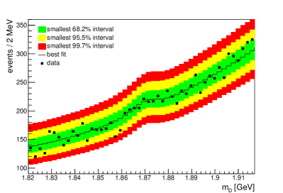
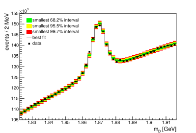
Figure 1 shows the invariant-mass distributions of the data for the five- and four-particle decays with the results of the fits shown as bands of posterior probability corresponding to the typically given one-, two-, and three-standard-deviation intervals. We see that the fits describe the data well. They determine the signal yields to be $($\fpeval{8474*0.0181}$\pm$\fpeval{8474*0.0082843}$)$ ​$\mathrm{e}\mathrm{v}\mathrm{e}\mathrm{n}\mathrm{t}\mathrm{s}$ for the five-particle decay and $($\fpeval{5929690*0.0238788}$\pm$\fpeval{5929690*0.000240931}$)$ ​$\mathrm{e}\mathrm{v}\mathrm{e}\mathrm{n}\mathrm{t}\mathrm{s}$ for the four-particle decay. The uncertainties are statistical only.

Figure 1: Invariant mass distributions of $\mathit{{D}{}_{\mspace{-3.0mu}\scriptstyle{}}^{\mspace{-1.0mu}\scriptstyle{+}}}$ candidates in ${\mathit{{D}{}_{\mspace{-3.0mu}\scriptstyle{}}^{\mspace{-1.0mu}\scriptstyle{+}}}\!\!\to{{\mathit{{K}{}_{\mspace{-3.0mu}\scriptstyle{}}^{\mspace{-1.0mu}\scriptstyle{-}}}\!\mathit{{K}{}_{\mspace{-3.0mu}\scriptstyle{}}^{\mspace{-1.0mu}\scriptstyle{}}}^{0}_{\text{S}}\;\!\mathit{{\pi}{}_{\mspace{-3.0mu}\scriptstyle{}}^{\mspace{-1.0mu}\scriptstyle{+}}}\!\mathit{{\pi}{}_{\mspace{-3.0mu}\scriptstyle{}}^{\mspace{-1.0mu}\scriptstyle{+}}}}\!\mathit{{\pi}{}_{\mspace{-3.0mu}\scriptstyle{}}^{\mspace{-1.0mu}\scriptstyle{}}}^{0}}}$ (top) and ${\mathit{{D}{}_{\mspace{-3.0mu}\scriptstyle{}}^{\mspace{-1.0mu}\scriptstyle{+}}}\!\!\to{\mathit{{K}{}_{\mspace{-3.0mu}\scriptstyle{}}^{\mspace{-1.0mu}\scriptstyle{-}}}\!\mathit{{K}{}_{\mspace{-3.0mu}\scriptstyle{}}^{\mspace{-1.0mu}\scriptstyle{}}}^{0}_{\text{S}}\;\!\mathit{{\pi}{}_{\mspace{-3.0mu}\scriptstyle{}}^{\mspace{-1.0mu}\scriptstyle{+}}}\!\mathit{{\pi}{}_{\mspace{-3.0mu}\scriptstyle{}}^{\mspace{-1.0mu}\scriptstyle{+}}}}}$ (bottom) of the data (dots). The results of the unbinned fits are projected into the same bins as the data at the best fit point (line) and as bands of posterior probability for the observed number of events. The vertical axes start from nonzero values to highlight the shapes of the data and models.

After the $\mathit{{\eta}{}_{\mspace{-3.0mu}\scriptstyle{}}^{\mspace{-1.0mu}\scriptstyle{}}}$ and $\mathit{{\omega}{}_{\mspace{-3.0mu}\scriptstyle{}}^{\mspace{-1.0mu}\scriptstyle{}}}$ vetoes, the five-particle signal-like yield still contains some $\overline{K}^{*0}\mathit{{\eta}{}_{\mspace{-3.0mu}\scriptstyle{}}^{\mspace{-1.0mu}\scriptstyle{}}}\mathit{{\pi}{}_{\mspace{-3.0mu}\scriptstyle{}}^{\mspace{-1.0mu}\scriptstyle{+}}}$ and $\overline{K}^{*0}\mathit{{\omega}{}_{\mspace{-3.0mu}\scriptstyle{}}^{\mspace{-1.0mu}\scriptstyle{}}}\mathit{{\pi}{}_{\mspace{-3.0mu}\scriptstyle{}}^{\mspace{-1.0mu}\scriptstyle{+}}}$ events. Although we can precisely estimate our suppression of this component, we cannot estimate its size after suppression since the branching fractions for decay to ${\mathit{{\mkern 4.0mu\overline{\mkern-4.0mu{K}}}{}_{\mspace{-2.0mu}\scriptstyle{}}^{\mspace{0.0mu}\scriptstyle{*}}}\!\!\;\mathit{{\eta}{}_{\mspace{-3.0mu}\scriptstyle{}}^{\mspace{-1.0mu}\scriptstyle{}}}\!\;\mathit{{\pi}{}_{\mspace{-3.0mu}\scriptstyle{}}^{\mspace{-1.0mu}\scriptstyle{+}}}}$ or ${\mathit{{\mkern 4.0mu\overline{\mkern-4.0mu{K}}}{}_{\mspace{-2.0mu}\scriptstyle{}}^{\mspace{0.0mu}\scriptstyle{*}}}\!\!\;\mathit{{\omega}{}_{\mspace{-3.0mu}\scriptstyle{}}^{\mspace{-1.0mu}\scriptstyle{}}}\!\;\mathit{{\pi}{}_{\mspace{-3.0mu}\scriptstyle{}}^{\mspace{-1.0mu}\scriptstyle{+}}}}$ are poorly measured Barlag et al. (1992). Using the signal yield from a fit without the $\mathit{{\eta}{}_{\mspace{-3.0mu}\scriptstyle{}}^{\mspace{-1.0mu}\scriptstyle{}}}$ and $\mathit{{\omega}{}_{\mspace{-3.0mu}\scriptstyle{}}^{\mspace{-1.0mu}\scriptstyle{}}}$ vetoes, $y$, we can determine $Y_{5}$, which is needed for the branching fraction determination:

$$Y_{5}=\frac{\epsilon_{5}^{\text{v}}}{\epsilon_{5}^{\text{v}}-\epsilon_{\mathit{{\eta}{}_{\mspace{-3.0mu}\scriptstyle{}}^{\mspace{-1.0mu}\scriptstyle{}}}\mathit{{\omega}{}_{\mspace{-3.0mu}\scriptstyle{}}^{\mspace{-1.0mu}\scriptstyle{}}}}^{\text{v}}}\quantity(Y-\epsilon_{\mathit{{\eta}{}_{\mspace{-3.0mu}\scriptstyle{}}^{\mspace{-1.0mu}\scriptstyle{}}}\mathit{{\omega}{}_{\mspace{-3.0mu}\scriptstyle{}}^{\mspace{-1.0mu}\scriptstyle{}}}}^{\text{v}}y),$$ (4)

where $Y$ is the signal yield with the vetoes, given above, and $\epsilon_{5}^{\text{v}}$ and $\epsilon_{\mathit{{\eta}{}_{\mspace{-3.0mu}\scriptstyle{}}^{\mspace{-1.0mu}\scriptstyle{}}}\mathit{{\omega}{}_{\mspace{-3.0mu}\scriptstyle{}}^{\mspace{-1.0mu}\scriptstyle{}}}}^{\text{v}}$ are the efficiencies of the vetoes (given earlier) for the signal and the decays to ${\mathit{{\mkern 4.0mu\overline{\mkern-4.0mu{K}}}{}_{\mspace{-2.0mu}\scriptstyle{}}^{\mspace{0.0mu}\scriptstyle{*}}}\!\!\;\mathit{{\eta}{}_{\mspace{-3.0mu}\scriptstyle{}}^{\mspace{-1.0mu}\scriptstyle{}}}\!\;\mathit{{\pi}{}_{\mspace{-3.0mu}\scriptstyle{}}^{\mspace{-1.0mu}\scriptstyle{+}}}}$ or ${\mathit{{\mkern 4.0mu\overline{\mkern-4.0mu{K}}}{}_{\mspace{-2.0mu}\scriptstyle{}}^{\mspace{0.0mu}\scriptstyle{*}}}\!\!\;\mathit{{\omega}{}_{\mspace{-3.0mu}\scriptstyle{}}^{\mspace{-1.0mu}\scriptstyle{}}}\!\;\mathit{{\pi}{}_{\mspace{-3.0mu}\scriptstyle{}}^{\mspace{-1.0mu}\scriptstyle{+}}}}$ determined from simulated data. The fit without the vetoes yields $($\fpeval{14682*0.026388}$\pm$\fpeval{14682*0.0067257}$)$ ​$\mathrm{e}\mathrm{v}\mathrm{e}\mathrm{n}\mathrm{t}\mathrm{s}$. The signal yield $Y_{5}$ (in the fit with vetoes) is $($136.615$\pm$81.8702$)$ ​$\mathrm{e}\mathrm{v}\mathrm{e}\mathrm{n}\mathrm{t}\mathrm{s}$. 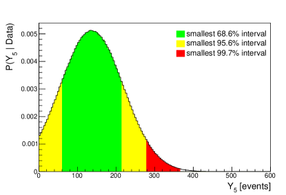Figure 2 shows the posterior probability distribution for $Y_{5}$. The posterior is normal, but cut off by its physical lower limit, zero.

Figure 2: Posterior probability distribution for the true five-particle signal yield.

Since we calculate the branching fraction from the ratio $\ifrac{Y_{5}}{Y_{4}}$, many systematic uncertainties related to particle detection and identification cancel to negligible values. The systematic uncertainty on the relative branching fraction comes from two sources: the detection of the $\mathit{{\pi}{}_{\mspace{-3.0mu}\scriptstyle{}}^{\mspace{-1.0mu}\scriptstyle{}}}^{0}$ in the five-particle decay and the estimation of the efficiency.

The systematic uncertainty arising from $\mathit{{\pi}{}_{\mspace{-3.0mu}\scriptstyle{}}^{\mspace{-1.0mu}\scriptstyle{}}}^{0}$ detection has been studied in $\mathit{{\tau}{}_{\mspace{-3.0mu}\scriptstyle{}}^{\mspace{-1.0mu}\scriptstyle{-}}}\mspace{1.0mu}\to\mspace{1.0mu}\mathit{{\pi}{}_{\mspace{-3.0mu}\scriptstyle{}}^{\mspace{-1.0mu}\scriptstyle{-}}}\mathit{{\pi}{}_{\mspace{-3.0mu}\scriptstyle{}}^{\mspace{-1.0mu}\scriptstyle{}}}^{0}\mathit{{\nu}{}_{\mspace{-3.0mu}\scriptstyle{\!\tau}}^{\mspace{-1.0mu}\scriptstyle{}}}$. For neutral pions in our momentum range (near or below $500\text{\,}\mathrm{M}\mathrm{e}\mathrm{V}$), the relative systematic uncertainty is $2.3\text{\,}\!\mathrm{\char 37\relax}$.

The efficiency for detecting the five particle state depends greatly on where events are distributed in the phase space available to the decay. This distribution depends on what intermediate resonances (and what spin configurations thereof) there are between the $\mathit{{D}{}_{\mspace{-3.0mu}\scriptstyle{}}^{\mspace{-1.0mu}\scriptstyle{+}}}$ and the final state. Since the efficiency is most sensitive to the $\mathit{{\pi}{}_{\mspace{-3.0mu}\scriptstyle{}}^{\mspace{-1.0mu}\scriptstyle{}}}^{0}$ momentum, we map the efficiency (from simulated data) in the two-dimensional plane of the squared invariant mass of the $\mathit{{\pi}{}_{\mspace{-3.0mu}\scriptstyle{}}^{\mspace{-1.0mu}\scriptstyle{+}}}\mathit{{\pi}{}_{\mspace{-3.0mu}\scriptstyle{}}^{\mspace{-1.0mu}\scriptstyle{+}}}\mathit{{\pi}{}_{\mspace{-3.0mu}\scriptstyle{}}^{\mspace{-1.0mu}\scriptstyle{}}}^{0}$ system versus the squared invariant mass of the $\mathit{{K}{}_{\mspace{-3.0mu}\scriptstyle{}}^{\mspace{-1.0mu}\scriptstyle{-}}}\mathit{{K}{}_{\mspace{-3.0mu}\scriptstyle{}}^{\mspace{-1.0mu}\scriptstyle{}}}^{0}_{\text{S}}\mathit{{\pi}{}_{\mspace{-3.0mu}\scriptstyle{}}^{\mspace{-1.0mu}\scriptstyle{}}}^{0}$ system. The efficiency is calculated in bins of this plane from simulated data in which the five final-state particles are uniformly distributed in the available phase space. The efficiency used to calculate the branching fraction is a sum of the values in these bins weighted by the distribution of events evenly distributed in phase space.

To calculate the systematic uncertainty arising from nature having a different distribution in phase space than what we use to calculate the efficiency, we calculate the efficiency for three further models of the decay: via $\mathit{{K}{}_{\mspace{-3.0mu}\scriptstyle{}}^{\mspace{-1.0mu}\scriptstyle{*+}}}\mathit{{K}{}_{\mspace{-3.0mu}\scriptstyle{}}^{\mspace{-1.0mu}\scriptstyle{*-}}}\mathit{{\pi}{}_{\mspace{-3.0mu}\scriptstyle{}}^{\mspace{-1.0mu}\scriptstyle{+}}}$, via $\mathit{{K}{}_{\mspace{-3.0mu}\scriptstyle{}}^{\mspace{-1.0mu}\scriptstyle{}}}^{*0}\overline{K}^{*0}\mathit{{\pi}{}_{\mspace{-3.0mu}\scriptstyle{}}^{\mspace{-1.0mu}\scriptstyle{+}}}$, and via $\mathit{{K}{}_{\mspace{-3.0mu}\scriptstyle{}}^{\mspace{-1.0mu}\scriptstyle{*+}}}\overline{K}^{*0}\mathit{{\pi}{}_{\mspace{-3.0mu}\scriptstyle{}}^{\mspace{-1.0mu}\scriptstyle{}}}^{0}$, with the three particles of each model distributed uniformly in the available (three-particle) phase space. We take the spread of the efficiencies as a systematic uncertainty. The resulting relative systematic uncertainty is asymmetric: $+12.6038\text{\,}\!\mathrm{\char 37\relax}$ and $-6.4428\text{\,}\!\mathrm{\char 37\relax}$.

We sum both systematic uncertainties in quadrature, yielding a total systematic uncertainty of $+\fpeval{sqrt(12.6038^{2}+2.3^{2})}\text{\,}\!\mathrm{\char 37\relax}$ and $-\fpeval{sqrt(6.4428^{2}+2.3^{2})}\text{\,}\!\mathrm{\char 37\relax}$.

The above values yield a branching fraction for the five-particle decay

$$\mathcal{B}({{\mathit{{K}{}_{\mspace{-3.0mu}\scriptstyle{}}^{\mspace{-1.0mu}\scriptstyle{-}}}\!\mathit{{K}{}_{\mspace{-3.0mu}\scriptstyle{}}^{\mspace{-1.0mu}\scriptstyle{}}}^{0}_{\text{S}}\;\!\mathit{{\pi}{}_{\mspace{-3.0mu}\scriptstyle{}}^{\mspace{-1.0mu}\scriptstyle{+}}}\!\mathit{{\pi}{}_{\mspace{-3.0mu}\scriptstyle{}}^{\mspace{-1.0mu}\scriptstyle{+}}}}\!\mathit{{\pi}{}_{\mspace{-3.0mu}\scriptstyle{}}^{\mspace{-1.0mu}\scriptstyle{}}}^{0}})=\quantity($6.353$\,\pm$3.778$\,^{$+\fpeval{6.353*\fpeval{sqrt(12.6038^{2}+2.3^{2})}/100}$}_{$-\fpeval{6.353*\fpeval{sqrt(6.4428^{2}+2.3^{2})}/100}$}\pm$\fpeval{6.353*\fpeval{0.17/2.27*100}/100}$)\times${10}^{-5}$,$$ (5)

where the first uncertainty is statistical, the second is systematic, and the third is from the uncertainty on the four-particle branching fraction Zyla et al. (2020). Compared to the hypothesis of there being no five-particle decay, this result has a significance of $1.68908$ standard deviations.

Equation (4), along with $Y=Y_{5}+Y_{\mathit{{\eta}{}_{\mspace{-3.0mu}\scriptstyle{}}^{\mspace{-1.0mu}\scriptstyle{}}}\mathit{{\omega}{}_{\mspace{-3.0mu}\scriptstyle{}}^{\mspace{-1.0mu}\scriptstyle{}}}}$, gives us the combined yield for decay to ${\mathit{{\mkern 4.0mu\overline{\mkern-4.0mu{K}}}{}_{\mspace{-2.0mu}\scriptstyle{}}^{\mspace{0.0mu}\scriptstyle{*}}}\!\!\;\mathit{{\eta}{}_{\mspace{-3.0mu}\scriptstyle{}}^{\mspace{-1.0mu}\scriptstyle{}}}\!\;\mathit{{\pi}{}_{\mspace{-3.0mu}\scriptstyle{}}^{\mspace{-1.0mu}\scriptstyle{+}}}}$ or ${\mathit{{\mkern 4.0mu\overline{\mkern-4.0mu{K}}}{}_{\mspace{-2.0mu}\scriptstyle{}}^{\mspace{0.0mu}\scriptstyle{*}}}\!\!\;\mathit{{\omega}{}_{\mspace{-3.0mu}\scriptstyle{}}^{\mspace{-1.0mu}\scriptstyle{}}}\!\;\mathit{{\pi}{}_{\mspace{-3.0mu}\scriptstyle{}}^{\mspace{-1.0mu}\scriptstyle{+}}}}$ in our data. We can calculate the sum of branching fractions for both decays:

$$\mathcal{B}({\mathit{{\mkern 4.0mu\overline{\mkern-4.0mu{K}}}{}_{\mspace{-2.0mu}\scriptstyle{}}^{\mspace{0.0mu}\scriptstyle{*}}}\!\!\;\mathit{{\eta}{}_{\mspace{-3.0mu}\scriptstyle{}}^{\mspace{-1.0mu}\scriptstyle{}}}\!\;\mathit{{\pi}{}_{\mspace{-3.0mu}\scriptstyle{}}^{\mspace{-1.0mu}\scriptstyle{+}}}})+\mathcal{B}({\mathit{{\mkern 4.0mu\overline{\mkern-4.0mu{K}}}{}_{\mspace{-2.0mu}\scriptstyle{}}^{\mspace{0.0mu}\scriptstyle{*}}}\!\!\;\mathit{{\omega}{}_{\mspace{-3.0mu}\scriptstyle{}}^{\mspace{-1.0mu}\scriptstyle{}}}\!\;\mathit{{\pi}{}_{\mspace{-3.0mu}\scriptstyle{}}^{\mspace{-1.0mu}\scriptstyle{+}}}})=\quantity($6.01831$\,^{$+6.23941$}_{$-5.74372$}\,{}^{$+\fpeval{6.01831*\fpeval{sqrt(12.6038^{2}+2.3^{2})}/100}$}_{$-\fpeval{6.01831*\fpeval{sqrt(6.4428^{2}+2.3^{2})}/100}$}\pm$\fpeval{6.01831*\fpeval{0.17/2.27*100}/100}$)\times${10}^{-5}$$$ (6)

where we have used the (combined) efficiency for these channels, $($5.27243$\pm$0.6$)$ ​$\times$${10}^{-5}$. The uncertainties are as given in equation (5). The statistical correlation of this value with that given in equation (5) is $-0.797376$. The systematic uncertainties are fully correlated between both values. This value is consistent with zero as is the previous measurement, by the ACCMOR collaboration, of ${\mathit{{D}{}_{\mspace{-3.0mu}\scriptstyle{}}^{\mspace{-1.0mu}\scriptstyle{+}}}\!\!\to{\mathit{{K}{}_{\mspace{-3.0mu}\scriptstyle{}}^{\mspace{-1.0mu}\scriptstyle{-}}}\!\mathit{{\pi}{}_{\mspace{-3.0mu}\scriptstyle{}}^{\mspace{-1.0mu}\scriptstyle{+}}}\!\mathit{{\pi}{}_{\mspace{-3.0mu}\scriptstyle{}}^{\mspace{-1.0mu}\scriptstyle{+}}}\!\mathit{{\pi}{}_{\mspace{-3.0mu}\scriptstyle{}}^{\mspace{-1.0mu}\scriptstyle{+}}}\!\mathit{{\pi}{}_{\mspace{-3.0mu}\scriptstyle{}}^{\mspace{-1.0mu}\scriptstyle{-}}}\!\mathit{{\pi}{}_{\mspace{-3.0mu}\scriptstyle{}}^{\mspace{-1.0mu}\scriptstyle{}}}^{0}}}$ (excluding $\mathit{{K}{}_{\mspace{-3.0mu}\scriptstyle{}}^{\mspace{-1.0mu}\scriptstyle{}}}^{0}_{\text{S}}$, but not selecting for $\mathit{{\eta}{}_{\mspace{-3.0mu}\scriptstyle{}}^{\mspace{-1.0mu}\scriptstyle{}}}$ or $\mathit{{\omega}{}_{\mspace{-3.0mu}\scriptstyle{}}^{\mspace{-1.0mu}\scriptstyle{}}}$) and has an uncertainty more than order of magnitude smaller than that reported by ACCMOR Barlag et al. (1992). Compared to the hypothesis of there being no such decay, this result has a significance of $1.09243$. By integrating the sampled posterior distribution, we calculate its upper limit at $95\text{\,}\!\mathrm{\char 37\relax}$ credibility is $1.7561\text{\times}{10}^{-4}$. Our study was not optimized for this channel. To definitively measure it, one should conduct a dedicated search with a $\mathit{{K}{}_{\mspace{-3.0mu}\scriptstyle{}}^{\mspace{-1.0mu}\scriptstyle{}}}^{0}_{\text{S}}$ veto instead of a $\mathit{{K}{}_{\mspace{-3.0mu}\scriptstyle{}}^{\mspace{-1.0mu}\scriptstyle{}}}^{0}_{\text{S}}$ selection.

IV Conclusion

We used $988\text{\,}\mathrm{f}\mathrm{b}^{-1}$ of data collected by the Belle experiment to measure the branching fraction for ${\mathit{{D}{}_{\mspace{-3.0mu}\scriptstyle{}}^{\mspace{-1.0mu}\scriptstyle{+}}}\!\!\to{{\mathit{{K}{}_{\mspace{-3.0mu}\scriptstyle{}}^{\mspace{-1.0mu}\scriptstyle{-}}}\!\mathit{{K}{}_{\mspace{-3.0mu}\scriptstyle{}}^{\mspace{-1.0mu}\scriptstyle{}}}^{0}_{\text{S}}\;\!\mathit{{\pi}{}_{\mspace{-3.0mu}\scriptstyle{}}^{\mspace{-1.0mu}\scriptstyle{+}}}\!\mathit{{\pi}{}_{\mspace{-3.0mu}\scriptstyle{}}^{\mspace{-1.0mu}\scriptstyle{+}}}}\!\mathit{{\pi}{}_{\mspace{-3.0mu}\scriptstyle{}}^{\mspace{-1.0mu}\scriptstyle{}}}^{0}}}$, whose precision is dominated by its statistical uncertainty. We do not observe statistically significant evidence for the occurrence of the decay and therefore report its upper limit at $95\text{\,}\!\mathrm{\char 37\relax}$ credibility:

$$\mathcal{B}({{\mathit{{K}{}_{\mspace{-3.0mu}\scriptstyle{}}^{\mspace{-1.0mu}\scriptstyle{-}}}\!\mathit{{K}{}_{\mspace{-3.0mu}\scriptstyle{}}^{\mspace{-1.0mu}\scriptstyle{}}}^{0}_{\text{S}}\;\!\mathit{{\pi}{}_{\mspace{-3.0mu}\scriptstyle{}}^{\mspace{-1.0mu}\scriptstyle{+}}}\!\mathit{{\pi}{}_{\mspace{-3.0mu}\scriptstyle{}}^{\mspace{-1.0mu}\scriptstyle{+}}}}\!\mathit{{\pi}{}_{\mspace{-3.0mu}\scriptstyle{}}^{\mspace{-1.0mu}\scriptstyle{}}}^{0}})<$1.36396\text{\times}{10}^{-4}$.$$ (7)

The Belle II experiment aims to collect fifty times more integrated luminosity than Belle. With such an increase of data, definitive observation of a branching fraction as small as a few ${10}^{-5}$ will be possible or an upper limit at order ${10}^{-5}$ can be established.