Nonparametric Bayesian Approach to Treatment Ranking in Network Meta-Analysis with Application to Comparisons of Antidepressants

Abstract

Network meta-analysis is a powerful tool to synthesize evidence from independent studies and compare multiple treatments simultaneously. A critical task of performing a network meta-analysis is to offer ranks of all available treatment options for a specific disease outcome. Frequently, the estimated treatment rankings are accompanied by a large amount of uncertainty, suffer from multiplicity issues, and rarely permit ties. These issues make interpreting rankings problematic as they are often treated as absolute metrics. To address these shortcomings, we formulate a ranking strategy that adapts to scenarios with high order uncertainty by producing more conservative results. This improves the interpretability while simultaneously accounting for multiple comparisons. To admit ties between treatment effects, we also develop a Bayesian Nonparametric approach for network meta-analysis. The approach capitalizes on the induced clustering mechanism of Bayesian Nonparametric methods producing a positive probability that two treatment effects are equal. We demonstrate the utility of the procedure through numerical experiments and a network meta-analysis designed to study antidepressant treatments.

Key words: multiple comparisons, network meta-analysis, nonparametric Bayesian approach, stick-breaking process, spike and slab, treatment ranking.

1 Introduction

Network meta-analysis (NMA) is a powerful tool to synthesize evidence from independent studies and compare multiple treatments simultaneously (Lumley,, 2002; Lu and Ades,, 2004; Salanti,, 2012). It has been increasingly used in comparative effectiveness research and evidence-based medicine for making reliable medical decisions (Cipriani et al.,, 2013; Mills et al.,, 2013; Hutton et al.,, 2015; Riley et al.,, 2017). Compared with conventional pairwise meta-analyses that rely on direct comparisons, an NMA synthesizes both direct and indirect evidence and thus typically produces more precise treatment effect estimates (Jackson et al.,, 2017; Lin et al.,, 2019).

An attractive feature of an NMA is that it can yield coherent rankings of all available treatments for a specific disease outcome (Higgins and Welton,, 2015). Such rankings offer an intuitive way for clinicians to select optimal treatments. Salanti et al., (2011) proposed the surface under the cumulative ranking curve (SUCRA) to quantitatively summarize the performance of treatments in an NMA. The SUCRA has been increasingly reported in recent NMAs for quantifying treatment rankings (Petropoulou et al.,, 2017), and it has been advocated in the reporting guideline of NMAs (Hutton et al.,, 2015). This measure ranges from 0 to 1; a higher value indicates a better treatment performance. Alternative ranking methods, such as the P-score, have been studied in the recent evidence synthesis literature (Rücker and Schwarzer,, 2015, 2017; Mavridis et al.,, 2020; Rosenberger et al.,, 2021).

Despite their wide use in the current NMAs, the SUCRA and other existing treatment ranking measures have been criticized due to their potentially large uncertainties (Trinquart et al.,, 2016). For example, it is unclear whether the difference is substantial between a treatment with SUCRA=0.80 and another with SUCRA=0.75. Clinicians may misinterpret these treatment ranking measures as absolute metrics, and their uncertainties may be overlooked in clinical practice. Few studies have been devoted to account for uncertainties of treatment ranking measures (Veroniki et al.,, 2018; Wu et al.,, 2021).

Another critical problem of interpreting treatment rankings in an NMA is the multiplicity issue (Efthimiou and White,, 2020). This issue is due to the nature of NMAs: an NMA compares multiple treatments simultaneously, essentially leading to a problem of multiple hypothesis testings, while clinicians frequently interpret the effect estimate of each pair of treatment comparison separately, and thus the false positive rates could be seriously inflated. For example, consider a study with multiple treatments, labeled 1 to 10, that are compared to a placebo. Suppose that the effect is quantified by the mean difference, and all treatments actually have no effects compared with the placebo, so all mean differences have a true value of 0. We also assume that the mean differences independently follow standard normal distributions for convenience. In a conventional pairwise meta-analysis for treatment 1 vs. placebo, the probability of observing a mean difference of at least 1 is 15.9%. If we consider the comparisons of treatment 2 vs. placebo and treatment 3 vs. placebo simultaneously, then the probability of observing the best treatment with a mean difference of at least 1 becomes 29.2%. If we further consider all ten comparisons with placebo, then the probability of observing the best treatment with a mean difference of at least 1 becomes 82.2%. As such, in an NMA with more treatment comparisons, we are more likely to observe exaggerated treatment effects.

In addition, traditional Bayesian approaches for NMA do not provide tools that can be used to formally test equality between treatments. In an NMA, clinicians are first interested in determining that there is indeed a difference between treatments and, if so, then estimating the effect size. Traditional Bayesian approaches are not capable of testing for equality between treatments because the prior distributions employed do not put a positive probability on ties, that is, the event that two treatments are equal.

To overcome the foregoing limitations of existing NMA methods, we develop an ordering method based on ideas that are similar in spirit to that by Barrientos et al., (2021) that accounts for multiplicity and develops a Bayesian nonparametric (BNP) approach that allows ties with positive probability. Our approach orders treatment effects so that order uncertainty and multiple comparisons are deliberately considered. This is done by sequentially identifying ordering sets that have high posterior probabilities. As a result, order uncertainty is rationally included by remaining silent about the order of specific units when the uncertainty associated with their treatment estimates is high. When comparing treatment effects, we not only focus on whether a treatment effect is greater or less than another one but also on whether they are equal (i.e., ties are permitted). This requires a prior that places a positive probability on the event that two treatments have equal effects. For this reason, we develop a novel BNP approach to modeling treatment effects in an NMA. Our BNP model employs a spike and slab base measure (Kim et al.,, 2009; Canale et al.,, 2017), which permits us to easily incorporate ties among treatments in our rankings.

This article is organized as follows. Section 2.1 describes an NMA dataset of antidepressant comparisons originally reported by Cipriani et al., (2009), which will be used to illustrate the structure of NMA and serve as a real-world data analysis. Section 2.2 details a commonly-used model for performing an NMA. This article will consider the contrast-based framework that focuses on estimating treatment contrasts, while the literature also has extensive discussions on the use of arm-based NMA models (Dias and Ades,, 2016; Hong et al.,, 2016; Lin et al.,, 2017; White et al.,, 2019). Section 3 describes our approach to ordering treatment statements in a traditional NMA setting. This motivates proposing alternative models, which are described in Section 4. We then compare the performance from our new method to that of existing methods using simulation studies in Section 5 and, in Section 6, we compare methods using the antidepressants dataset. Finally, this article concludes with a brief discussion in Section 7.

2 Preliminaries

2.1 Description of Antidepressants Dataset

We use a dataset of antidepressants, originally reported by Cipriani et al., (2009), to illustrate the conventional NMA models and our proposed models. The dataset is comprised of 111 randomized controlled trials on major depression with 12 unique drug treatments. The original systematic review considered both the efficacy (reflected by response rate) and acceptability (reflected by dropout rate) outcomes. This article is restricted to NMA methods for a single outcome, instead of jointly modeling multiple outcomes; we focused on the efficacy outcome, which is binary. In our analysis, we label the 12 treatments in alphabetical order: 1) bupropion; 2) citalopram; 3) duloxetine; 4) escitalopram; 5) fluoxetine; 6) fluvoxamine; 7) milnacipran; 8) mirtazapine; 9) paroxetine; 10) reboxetine; 11) sertraline; and 12) venlafaxine. The odds ratio is used as the effect measure. For the efficacy outcome, the odds ratio of A vs. B higher than 1 indicates that treatment A performs better than treatment B.

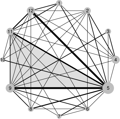
Figure 1: Network plot of the dataset of antidepressants. Each node represents an antidepressant, and each edge represents a direct comparison between the corresponding two antidepressants. The node size is proportional to the total sample size in the corresponding groups of antidepressants across studies, and the edge width is proportional to the number of studies that directly compare the corresponding antidepressants. The shaded loop represents the three-arm studies.

Figure 1 presents the network plot of this dataset. All studies but two were two-arm trials, while the other two studies were three-arm trials, comparing treatments 5, 9, and 11. Fluoxetine (treatment 5) had been conventionally used as a reference antidepressant (Magni et al.,, 2013); as such, it involves the largest sample size and the largest number of trials, as indicated in the network plot. This network is generally well connected, with many direct comparisons for treatment pairs. Nevertheless, most pairs of treatments are directly informed by a limited number of trials, and some comparisons (e.g., treatments 1 vs. 2 and 2 vs. 3) lack direct evidence. The NMA approach provides a valuable way for synthesizing direct and indirect comparisons in the same analysis and offering a coherence ranking of all available antidepressants.

2.2 Contrast-Based Model for Network Meta-Analysis

An NMA is commonly carried out using either a contrast-based or arm-based approach (Zhang et al.,, 2014; Efthimiou et al.,, 2016). The key difference between these two approaches is that the contrast-based approach assumes that relative treatment effects are exchangeable across studies, while the arm-based approach assumes exchangeability across studies for absolute treatment effects. White et al., (2019) offer a detailed comparison between the two approaches. Our focus is the contrast-based approach because assuming exchangeability across studies for the relative treatment effects is more widely used in current evidence synthesis (Dias and Ades,, 2016).

For context, we detail the contrast-based NMA model used by Lu and Ades, (2004, 2006) for binary outcomes, as in the antidepressant dataset in Section 2.1. Let $N$ be the total number of studies and $K$ be the total number of unique treatments across all studies. We use $\mathcal{T}_{i}$ to denote the collection of treatments that are included in study $i$ ($i=1,\ldots,N$). Further, $y_{ik}$ denotes the number of event outcomes (“successes”) associated with treatment $k\in\mathcal{T}_{i}$ and $n_{ik}$ the number of trials. Next, for study $i$, we use $b_{i}\in\mathcal{T}_{i}$ to denote the baseline treatment while $\mathcal{T}^{-b_{i}}_{i}=\mathcal{T}_{i}\setminus\{b_{i}\}$ denotes the collection of treatments excluding the baseline treatment. With this notation, consider the following random-effects model:

$$y_{ik}|p_{ik} \overset{\text{ind}}{\sim}\mbox{Binomial}(n_{ik},p_{ik})\ \mbox{for $i=1,\ldots,N$ and $k\in\mathcal{T}_{i}$};$$ (1)

$${\rm logit}(p_{ik}) =\mu_{i,b_{i}}+\delta_{i,b_{i}k}\mathbb{I}(b_{i}\neq k)\ k\in\mathcal{T}_{i};$$ (2)

$$\mu_{i,b_{i}} \overset{\text{iid}}{\sim}\mbox{N}(m_{b},s_{b});$$ (3)

$$\delta_{i,b_{i}k}|d_{1b_{i}},d_{1k} \overset{\text{ind}}{\sim}\mbox{N}(d_{1k}-d_{1b_{i}},\tau),\ k\in\mathcal{T}^{-b_{i}}_{i};$$ (4)

$${\rm Corr}(\delta_{i,b_{i}k},\delta_{i,b_{i}h}) =\gamma=0.5,\ k,h\in\mathcal{T}^{-b_{i}}_{i},k\neq h;$$ (5)

$$\tau^{2} \sim\mbox{LogN}(m_{\ell},s_{\ell});$$ (6)

$$d_{1k} \stackrel{{\scriptstyle\text{iid}}}{{\sim}}\mbox{N}(m_{d},s_{d}),\ k=2,\ldots,K\ \mbox{with $d_{11}=0$}.$$ (7)

In this model, $p_{ik}$ represents the probability of success for treatment $k$ in study $i$, $\mu_{i,b_{i}}$ represents study $i$’s baseline treatment effect, $\delta_{i,b_{i}k}$ represents the effect of treatment $k$ to treatment $b_{i}$, $d_{1k}$ represents the mean effect of treatment $k$ vs. treatment 1, the reference treatment. Of note, the baseline treatments and the reference treatment are not necessarily the same. If there are more than two treatments in a particular study (i.e., a multi-arm study), then the treatment effects are correlated. The correlation coefficient is typically assumed to be 0.5 (Higgins and Whitehead,, 1996; Lu and Ades,, 2004). All roman letters correspond to prior parameters that are user-supplied. The model in Equations (1)–(7) is adopted from Lu and Ades, (2006), except they employ a uniform prior distribution for $\tau$. The log-Gaussian prior for $\tau^{2}$ in Equation (6) is an alternative informative prior that is studied in Turner et al., (2012). In what follows, we will refer to this model as the “Gaussian effects” model because the $d_{1k}$ parameters are modeled using a Gaussian distribution.

The Gaussian effects model assumes that direct evidence is consistent with indirect evidence. Specifically, the NMA synthesizes both direct evidence (comparisons of treatments that are within a study) and indirect evidence (comparisons of treatments that do not appear together in a study but have a common comparator). Comparisons between treatments and the reference (i.e., $d_{1k}$) are called “basic parameters,” while those that are linear combinations of the basic parameters (e.g., $d_{kk^{\prime}}=d_{1k^{\prime}}-d_{1k}$) are called “functional parameters”. Functional parameters must be able to be written in terms of basic parameters. Under the assumption of evidence consistency, both direct and indirect comparisons estimate the same parameter.

3 Treatment Effect Comparisons Using Directed Graphs

Once the Gaussian effects model is fit, inference regarding treatment effect order is often desired. The pairwise comparisons available from the Gaussian effects model facilitate ordering the treatment effects. However, the ordering inherits the potentially high uncertainty that may exist among a subset of pairwise comparisons. This problem is not explicitly addressed by traditional methods that summarize treatment comparisons in an NMA (Trinquart et al.,, 2016). In particular, the issues that traditional methods do not simultaneously address are the following: i) multiplicity (i.e., complications that accompany inference in the case that all comparisons co-occur simultaneously), ii) identifying comparisons that have low uncertainty, and iii) representing all comparisons simultaneously in a concise and interpretable way. We develop a novel approach that addresses all three issues. Our approach seeks to identify treatments or groups of treatments whose comparisons are accompanied by low uncertainty (or high posterior probability). We account for multiple treatment comparisons by attaching a single posterior probability that comparisons occur simultaneously. Then, we display the simultaneous comparisons using an easy-to-interpret network graph from which treatment rankings can be extracted.

Our approach summarizes the treatment effects in an NMA using a graphical structure. The nodes of a graph represent the $K$ treatments which are denoted by $\mathcal{T}=\{1,\ldots,K\}$. The graphs considered are directed graphs with random edges. We use $\mathcal{E}$ to denote the random graph. The domain of $\mathcal{E}$ is the collection of all graphs with edges representing a set of ordered pairs of nodes which in turn represent comparisons among the treatments. In other words,

• if $(j,k),(k,j)\in\mathcal{E}$, then $d_{1j}=d_{1k}$;

• if $(j,k)\in\mathcal{E}$ but $(k,j)\not\in\mathcal{E}$, then $d_{1j}<d_{1k}$.

As an example, let $K=7$ with $E=\{(1,2),(2,4),(4,2),(1,4),(1,6),(2,6),(3,7),(7,3)\}$ which results in

$$\Pr(\mathcal{E}=E|{\rm Data})=\Pr(d_{11}<d_{12}<d_{16},d_{11}<d_{14},d_{12}=d_{14},d_{13}=d_{17}|{\rm Data}).$$

Figure 2 displays the graph $(\mathcal{T},E)$ described above, where dashed one-directional arrows point toward the treatment with larger effect. For example, treatment 6 has a larger effect compared to treatment 2. Solid bi-directional arrows represent the case where two treatments have the same effect. For example, treatments 2 and 4 have the same effect as well as treatments 3 and 7. A pair of nodes without an arrow connecting them indicates that no statement is made between them; in our strategy, no arrow between two nodes implies there is considerable uncertainty when comparing the two treatments. The kind of treatment rankings that can be extracted from the directed graph in Figure 2 are that treatment 6 performs better than treatments 1 and 2, treatment 2 performs better than 1, treatments 2 and 4 have similar effects, and comparing treatment 6 to treatment 4 is inconclusive.

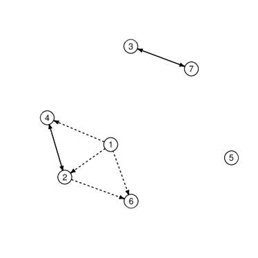
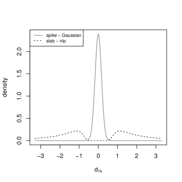
Figure 2: Illustrative plots. The left plot illustrates a network treatment effect when $K=7$ and $E=\{(1,2),(2,4),(4,2),(1,4),(1,6),(2,6),(3,7),(7,3)\}$. A dashed one-directional arrow from A to B indicates that treatment B performs better treatment A. A solid bi-directional arrow between A and B indicates that treatments A and B have the same effect. The right plot illustrates the spike and slab density where the spike is $N(0,v_{0}/3)$ and the slab is $\mbox{NLP}(p,1,1)$. The $p$ is selected so that $\mbox{NLP}(x_{0};p,1,1)=\mbox{N}(x_{0}|0,v_{0}/3)$, where $x_{0}$ satisfies $\int_{-x_{0}}^{x_{0}}\mbox{N}(x|0,v_{0}/3)dx\approx 0.999$.

Our goal is to find graphs like those displayed in Figure 2 that accumulate high posterior probability. This is accomplished by first creating a graph in which all nodes are connected through the relationship (e.g., $d_{1j}=d_{1k}$) that has the highest posterior probability. Jointly, the pairwise comparisons represented by this graph will typically have a low posterior probability. We then begin trimming the graph by removing arrows associated with relations that have the lowest posterior probability. This produces a sequence of graphs with varying amounts of informativeness and posterior probability, where larger posterior probability results in graphs that are more trimmed (less informative) and vice versa. To be more concrete, let

$$p_{j=k}=\Pr(d_{1j}=d_{1k}|{\rm Data}),\,p_{j<k}=\Pr(d_{1j}<d_{1k}|{\rm Data}),\,p_{j>k}=\Pr(d_{1j}>d_{1k}|{\rm Data}),$$

and define

$$\tilde{p}(j,k)=\max\{p_{j=k},\,p_{j<k},\,p_{j>k}\}$$

along with

$$e(j,k|\tilde{p})=\left\{\begin{array}[]{cl}\{(j,k),(k,j)\}&\mbox{if }p_{j=k}=\tilde{p}(j,k);\\ \{(j,k)\}&\mbox{if }p_{j<k}=\tilde{p}(j,k);\\ \{(k,j)\}&\mbox{if }p_{j>k}=\tilde{p}(j,k).\end{array}\right.$$

Here, $p(j,k)$ and $e(j,k)$ are computed under the assumption that $p_{j=k}$, $p_{j<k}$, and $p_{j>k}$ are all different. Under this assumption, $e(j,k)$ is uniquely determined. Based on $e(j,k)$, we now define an initial graph $\tilde{E}$ as

$$\tilde{E}=\bigcup_{j<k}e(j,k|\tilde{p}).$$

Before trimming $\tilde{E}$, we must verify that it represents a coherent set of treatment statements; that is, there is a transitive relation among the $K$ treatment effects. For example, if treatments $j$ and $k$ have the same effect and so do treatments $j$ and $l$, then treatments $k$ and $l$ also have the same effect; or if the treatment effect of $j$ is less than that of $k$ and treatments $j$ and $l$ have the same effect, then treatment $k$ has a smaller effect than treatment $l$. To verify the coherence of $\tilde{E}$, a sufficient condition is to check if ${\rm Pr}(\mathcal{E}=\tilde{E}|{\rm Data})>0$. This follows from the fact that the posterior distribution of $\mathcal{E}$ is supported on the space of all coherent graphs. If ${\rm Pr}(\mathcal{E}=\tilde{E}|{\rm Data})>0$ cannot be verified, we use the closest coherent graph to $\tilde{E}$, denoted as $E_{0}$, as the initial graph. Thus, the starting graph $E_{0}$ is defined as

$$E_{0}=\min_{\{E:\Pr(\mathcal{E}=E|{\rm Data})>0\}}d(\tilde{E},E)$$

with

$$d(\tilde{E},E) = \sum_{j<k}\left\{p_{j=k}\mathbb{I}_{\tilde{E}}(j,k)\mathbb{I}_{\tilde{E}}(k,j)\mathbb{I}_{E}(j,k)\mathbb{I}_{E}(k,j)\right.$$

$$\hskip 14.22636pt+\,p_{j<k}\mathbb{I}_{\tilde{E}}(j,k)(1-\mathbb{I}_{\tilde{E}}(k,j))[\mathbb{I}_{E}(j,k)\mathbb{I}_{E}(k,j)+2(1-\mathbb{I}_{E}(j,k))\mathbb{I}_{E}(k,j)]$$

$$\hskip 14.22636pt+\,\left.p_{j>k}(1-\mathbb{I}_{\tilde{E}}(j,k))\mathbb{I}_{\tilde{E}}(k,j)[\mathbb{I}_{E}(j,k)\mathbb{I}_{E}(k,j)+2\mathbb{I}_{E}(j,k)(1-\mathbb{I}_{E}(k,j))]\right\},$$

where $\mathbb{I}_{E}(j,k)=1$ if $(j,k)\in E$, and its equals 0 otherwise. Notice that $d(\cdot,\cdot)$ compares all edges in $\tilde{E}$ with those in $E$. If edges associated with treatment $j$ and $k$ have the same direction in $\tilde{E}$ and $E$ or are both bi-directional, then a value of 0 is assigned. If one edge is bi-directional and the other one is uni-directional, then a value of 1 is assigned to this comparison. If edges for $j$ and $k$ are uni-directional but with opposite directions, then a value of 2 is assigned to this comparison. The distance $d(\cdot,\cdot)$ is defined as a weighted sum of the values obtained for these comparisons, where $\tilde{p}(j,k)$ ($p_{j=k}$, $p_{j<k}$, or $p_{j>k}$) are used as weights. Using weights ensures that edges with high posterior probability are mostly retained.

As noted, our goal is to identify a collection of graphs $\{E_{\gamma}:\gamma\in[0,1]\}$ such that $p_{\gamma}=\Pr(\mathcal{E}=E_{\gamma}|{\rm Data})$ is an increasing function of $\gamma$. The idea is to define $E_{\gamma}\subseteq E_{0}$ as a graph comprised of a collection of pairwise comparisons (edges) that meet a certain probability threshold $\gamma$. We highlight the role that $\gamma$ plays in our formation of $E_{\gamma}$. As $\gamma\rightarrow 1$, $E_{\gamma}$ becomes more sparse (less informative); while as $\gamma\rightarrow 0$, $E_{\gamma}$ becomes $E_{0}$ (more informative). Our approach is to consider a sequence of thresholds (lower bounds) $\gamma\in[0,1]$ for the pairwise probabilities

$$E_{\gamma}=\bigcup_{(j,k):j<k,\,p(j,k)>\gamma}e(j,k|p),$$

where

$$p(i,j)=p_{j=k}\mathbb{I}_{E_{0}}(j,k)\mathbb{I}_{E_{0}}(k,j)+p_{j<k}\mathbb{I}_{E_{0}}(j,k)(1-\mathbb{I}_{E_{0}}(k,j))+p_{j>k}(1-\mathbb{I}_{E_{0}}(j,k))\mathbb{I}_{E_{0}}(k,j).$$

Users will then have access to $(E_{\gamma},p_{\gamma})$ for an increasing sequence of $\gamma_{1},\ldots,\gamma_{L}$ such that $E_{\gamma_{l}}\neq E_{\gamma_{l^{\prime}}}$ for every $l\neq l^{\prime}$. Users can then balance the posterior probability of graph vs. the sparsity of the graph for their particular setting.

With the Gaussian effects model described in Equations (1)–(7), it is not possible to formally test that two treatments have the same effect. As a result, using our approach to summarize treatment effect orderings would necessarily result in a graph that does not contain any bi-directional arrows. This motivates extending the Gaussian effects model so that ties between treatments are possible, which will be described in the next section.

4 Extensions to the Gaussian Effects Model

In this section, we provide details of an extension to the Gaussian effects model described in Section 2.2. The extension permits relaxing constraints highlighted in the previous section by allowing ties. In Section 4.1 we first detail a standard BNP approach that clusters $d_{1k}$, $2,\ldots,K$. Since the standard BNP approach does not allow clustering treatment $1$ (reference) along with the other treatments, in Section 4.2, we combine the standard BNP approach with spike and slab priors that allows clustering all treatments. Details associated with computation are provided in the online supplementary material.

4.1 Dirichlet Process Gaussian Effects Model

If ties are permitted, then $\Pr(d_{1k}=d_{1k^{\prime}})>0$. One way to incorporate this is to use a BNP method that induces a prior on the partitions of $\mathcal{T}$. BNP methods for partition modeling have exploded in popularity during the past decades. For sake of conciseness, we do not provide here a detailed review, but point interested readers to several book treatises, including Chapter 23 in Gelman et al., (2014), Müller et al., (2015), and Ghosal and van der Vaart, (2017). Our extension to the Gaussian effects model is to relax the assumption that $d_{1k}\sim N(m_{d},s_{d})$; we assume that $d_{1k}|\mathcal{P}\sim\mathcal{P}$ for some unknown density $\mathcal{P}$, and then assign a BNP prior to $\mathcal{P}$. The BNP prior we employ is the commonly used Dirichlet process (DP). Thus, we change Equation (7) to the following

$$d_{1k}|\mathcal{P} \stackrel{{\scriptstyle\text{iid}}}{{\sim}}\mathcal{P},\ k=2,\ldots,K,\ \mbox{with $d_{11}=0$},$$

$$\mathcal{P} \sim DP(\alpha,P_{0}),$$

$$P_{0} =\mbox{N}(m_{d},s_{d}).$$

Here, $DP(\alpha,P_{0})$ denotes a DP with concentration parameter $\alpha$ and base measure $P_{0}$. We refer to Equations (1)–(6) plus the prior described above as the “DP Gaussian effects” model.

The property of the DP that is of most interest to our current work is its almost surely discrete nature. A consequence of this property is that there is positive probability for ties among the $d_{1k}$. This is more easily seen by invoking the stick-breaking construction of a DP random probability measure (Sethuraman,, 1994), which dictates that $\mathcal{P}$ can be expressed as the following weighted sum of point masses $\mathcal{P}(\cdot)=\sum_{h=1}^{\infty}\pi_{h}\delta_{d^{\star}_{h}}(\cdot)$. Here, $\pi_{1},\pi_{2},\ldots$ denote probability weights such that $\pi_{h}=V_{h}\prod_{\ell<h}(1-V_{\ell})$ with $V_{h}\sim\mbox{Beta}(1,\alpha)$, and $\delta_{x}(\cdot)$ is the Dirac measure at $x$ with atoms $d^{\star}_{h}\sim P_{0}$. It is common, for computational reasons, to truncate the infinite mixture by some upper bound, say $H$ (Ishwaran and James,, 2001). Setting $V_{H}=1$ ensures that the weights still add to 1. In addition, it is common to introduce latent cluster labels $c_{k}$ such that $c_{k}=h$ implies that $d_{1k}=d^{\star}_{h}$ (or alternatively, $d_{1k}=d^{\star}_{c_{k}}$). Then, we can re-express the model for $d_{1k}$ in terms of the latent cluster labels as follows

$$d_{1k}|c_{k} \sim\delta_{d^{\star}_{c_{k}}},\ k=2,\ldots,K,\mbox{with $d_{11}=0$};$$

$$c_{k}|\pi_{1},\ldots,\pi_{H} \stackrel{{\scriptstyle\text{iid}}}{{\sim}}\sum_{h=1}^{H}\pi_{h}\delta_{h},\ k=2,\ldots,K;$$

$$d^{\star}_{h} \stackrel{{\scriptstyle\text{iid}}}{{\sim}}P_{0},\ h=1,\ldots,H,\ P_{0}=\mbox{N}(m_{d},s_{d}).$$

In this form, it is straightforward to see how our extension permits treatment effects to be equal with positive probability. Since $\Pr(c_{k}=c_{k^{\prime}})\neq 0$, we have that $\Pr(d^{\star}_{c_{k}}=d^{\star}_{c_{k^{\prime}}})=\Pr(d_{1k}=d_{1k^{\prime}})\neq 0$.

4.2 Dirichlet Process Spike-Slab Model

The appeal of the DP Gaussian effects model in our setting is that $\Pr(d_{1k}=d_{1k^{\prime}})>0$; as a result, we can consider ties. However, it is possible in an NMA that a subset of treatments have no effect, i.e., $d_{1k}=0$ for some $k\in\{2,\ldots,K\}$. Now, due to the Gaussian base measure employed in the DP Gaussian effects model, we have that $\Pr(d_{1k}=0)=0$. We next describe an extension to the DP Gaussian effects model that relaxes this constraint.

In order for $\Pr(d_{1k}=0)>0$, it is necessary that $\Pr(d^{\star}_{h}=0)>0$. Our approach to accommodating this characteristic is by using a spike and slab as the base measure of a DP. The spike and slab prior, which is commonly used in Bayesian variable selection (Mitchell and Beauchamp,, 1988; George and McCulloch,, 1993; Ishwaran and Rao,, 2005), is a two-component mixture model. The slab component is a relatively diffuse distribution typically centered at 0. The spike component is typically specified in one of two ways (Malsiner-Walli and Wagner,, 2011). One is to set the spike to a degenerate distribution at 0, while the other is to treat the spike as an absolutely continuous distribution centered at 0 with a small variance. In our formulation, we will use the latter. The reasons for doing so are two-folded. First, as mentioned by Canale et al., (2017), some BNP methods become more complex if the base measure has an atomic component. Second, and perhaps more importantly, using a continuous distribution with a small variance will give practitioners the ability to define a zero effect within the context of their study. That is, by setting the spike component to $\mbox{N}(0,v_{0}/3)$, $v_{0}$ is such that, if $d^{\star}_{h}\in(-v_{0},v_{0})$, then all treatments $k$ such that $c_{k}=h$ are assumed to have the same mean effect as treatment 1.

Using the spike and slab in BNP modeling has a presence in the literature (Kim et al.,, 2009; Scarpa and Dunson,, 2009; Canale et al.,, 2017). What sets us apart is our desire to have a spike with zero density for values in $(-\infty,-v_{0})\cup(v_{0},\infty)$ and slab with zero density for values in $(-v_{0},v_{0})$. To this end, for the slab component, we consider the inverse moment nonlocal prior density detailed in Johnson and Rossell, (2010). This density has the ability to put negligible mass on the neighborhood of a particular value (which for us is 0). For the sake of completeness, we list the density function here.

$$\mbox{NLP}(d^{\star}_{h}|p,r,u)=\frac{pr^{u/2}}{\Gamma(u/2p)}\{(d^{\star}_{h}-0)^{2}\}^{-(u+1)/2}\exp\left[-\left\{\frac{(d^{\star}_{h}-0)^{2}}{r}\right\}^{-p}\right].$$

We set $r=1$ and $u=1$ and select $p$ based on the user supplied $v_{0}$. The idea is to select $p$ so that $\mbox{N}(0,v_{0}/3)$ and $\mbox{NLP}(p,1,1)$ are 0 on $(-\infty,-v_{0})\cup(v_{0},\infty)$ and $(-v_{0},v_{0})$, respectively. To do so, we find $x_{0}$ such that $\int_{-x_{0}}^{x_{0}}\mbox{N}(x|0,v_{0}/3)dx\approx 0.999$ and then set $p>0$ to the value that produces $\mbox{NLP}(x_{0}|p,1,1)=\mbox{N}(x_{0}|0,v_{0}/3)$. An example of the the spike and slab densities we employ when $v_{0}=0.5$ is provided in the right plot of Figure 2. Notice that the overlap of density between the spike and slab is essentially 0.

With the foregoing details of the spike and slab base measure, the extension to the DP Gaussian effects model (which we call the DP Spike-Slab model) is the following:

$$d_{1k}|\mathcal{P} \stackrel{{\scriptstyle\text{iid}}}{{\sim}}\mathcal{P},\ k=2,\ldots,K\ \mbox{with $d_{11}=0$};$$

$$\mathcal{P} \sim DP(\alpha,P_{0});$$

$$P_{0} =\omega_{0}\mbox{N}(0,v_{0}/3)+(1-\omega_{0})\mbox{NLP}(p,1,1);$$

$$\omega_{0} \sim\mbox{Beta}(a_{\omega},b_{\omega}),$$

where $\omega_{0}$ is associated with $\Pr(d^{\star}_{h}=0)$, and $a_{\omega}$ and $b_{\omega}$ are user supplied. As with the DP Gaussian effects model, introducing latent component labels for the DP ($c_{k}$) and for the spike and slab ($s_{h}$) facilitate computation. After introducing both component labels, the DP Spike-Slab model can be re-expressed as

$$d_{1k}|c_{k} \stackrel{{\scriptstyle\text{ind}}}{{\sim}}\delta_{d^{\star}_{c_{k}}},\ k=2,\ldots,K,\mbox{with $d_{11}=0$};$$

$$c_{k}|\pi_{1},\ldots,\pi_{H} \stackrel{{\scriptstyle\text{iid}}}{{\sim}}\sum_{h=1}^{H}\pi_{h}\delta_{h},\ k=2,\ldots,K;$$

$$d^{\star}_{h}|s_{h} \sim\mbox{N}(0,v_{0}/3)^{s_{h}}~{}\mbox{NLP}(p,1,1)^{1-s_{h}},\ h=1,\ldots,H;$$

$$s_{h} \sim\mbox{Bernoulli}(\omega_{0}),\ h=1,\ldots,H;$$

$$\omega_{0} \sim\mbox{Beta}(a_{\omega},b_{\omega}),$$

where, once again, $p$ is determined by $v_{0}$.

5 Simulation Study

5.1 Simulation Designs

We conducted a simulation study to illustrate our approach and highlight its utility when there exist treatment effects that are similar and/or close to 0. We also explored the loss of efficiency if no such treatment effects exist. The treatment network design is based on that found in the antidepressant dataset described in Section 2.1. However, to make the simulation study more manageable, we only consider 6 of the 12 treatments, and this subset of treatments appear in $i=1,\ldots,55$ studies. Data were generated by fixing $d_{1k}$ for $k\in\{1,\ldots,6\}$ to specific values, which were then used to generate $\delta_{i,b_{i}k}$ that in turn produced values for $p_{ik}$. The $p_{ik}$ values were then used to generate the number of successes (i.e., $y_{ik}$) based on the number of trials (i.e., $n_{ik}$). The $n_{ik}$ values all came from the subset of the antidepressant dataset described in Section 2.1.

In the simulation, we studied the impact of three factors: (i) the signal-to-noise ratio; (ii) the effect/treatment structure; and (iii) the effect size. The signal vs. noise was controlled by $\tau$, and we considered $\tau\in\{0.05,0.1\}$. The effect/treatment structure was determined by the values of $\bm{d}_{1}$. In order to select reasonable values for $\bm{d}_{1}$, we fit the DP Spike-Slab model to the subset of the antidepressant dataset. The posterior mean of $\bm{d}_{1}$ from this fit was $(0,0.3,0.0,0.0,0.3,0.3)^{\prime}$, which is the basis of the three different $\bm{d}_{1}$ vectors that we employed. Each of the three $\bm{d}_{1}$ vectors was constructed to favor one of the three models under consideration (the Gaussian effects, DP Gaussian effects, or DP Spick-Slab models). Their exact forms are provided in the following enumerated list.

1. $\bm{d}_{1}=(0,-0.6,-0.3,0.3,0.6,0.9)^{\prime}$. This $\bm{d}_{1}$ vector favors the Gaussian effects model as all entries are different and none are equal to 0. We refer to this data generating scenario as “$\bm{d}_{1}\sim$ Gaussian.”

2. $\bm{d}_{1}=(0,0.3,-0.3,-0.3,0.3,0.3)^{\prime}$. This $\bm{d}_{1}$ vector favors the DP Gaussian effects model as there are two clusters of effects and none are equal to 0. We refer to this data generating scenario as “$\bm{d}_{1}\sim$ DP Gaussian.”

3. $\bm{d}_{1}=(0,0.3,0.0,0.0,0.3,0.3)^{\prime}$. This $\bm{d}_{1}$ vector favors the DP Spike-Slab model as there are two clusters with one setting the effects to 0. We refer to this data generating scenario as “$\bm{d}_{1}\sim$ DP Spike-Slab.”

Finally, to study the effect size, we multiplied each of the $\bm{d}_{1}$ vectors in the three scenarios above by 0 (which resulted in no nonzero effects), 1, and 2 (which corresponded to an effect size that was twice as large). For simplicity, these three “effect sizes” are called effect size 0, effect size 1, and effect size 2, respectively. In total, there were 18 data generating scenarios; under each scenario, 100 datasets were generated.

To each generated data set, we fit the Gaussian effects, DP Gaussian effects, and DP Spike-Slab models. For all three models, we set $m_{b}=0$, $s_{b}=10$, $m_{\ell}=-2.34$, and $s_{\ell}=2$. The later two prior values were selected based on suggestions from Turner et al., (2012). For the Gaussian effects and DP Gaussian effects models, we set $m_{d}=0$ and $s_{d}=1$. For the DP Gaussian effects and DP Spike-Slab models, we set $\alpha=1$. For the DP Spike-Slab model, we set $a_{\omega}=b_{\omega}=1$, and for the nonlocal prior component, we employed $v_{0}=0.05$. We also considered $v_{0}=0.1$ with results being almost identical. All model fits were carried out by running 5 independent MCMC chains each for 200,000 MCMC samples, of which the first 100,000 were discarded as burn-in and the remaining samples were thinned by 100. We were very liberal in the amount of burn-in and thinning to ensure that convergence was met and that independent (at least approximately) samples were collected. Combining the 5 chains resulted in a total of 5,000 MCMC samples.

5.2 Simulation Results

We compared the three methods’ performance by calculating posterior probabilities associated with the pairwise comparison graph determined by $\bm{d}_{1}$. We began by calculating the joint posterior probability of the true pairwise comparison graph in its entirety (i.e., all 15 comparisons jointly). Results are provided in Figure S.1 of the online supplementary material. Notice that when “$\bm{d}_{1}\sim$ Gaussian” was used to generate data and the effect size was 1 (i.e., the true vector $\bm{d}_{1}$ was multiplied by 1), the Gaussian effects model had a high probability of recovering the graph, while the DP Gaussian effects and DP Spike-Slab had much lower probabilities. This was expected as the data generating scenario favored the Gaussian effects model. However, as the effect size grew, the DP procedures performed on par with the Gaussian effects model, even when the Gaussian effects model had an advantage. When “$\bm{d}_{1}\sim$ DP Gaussian” was used to generate data, by construction, the Gaussian effects model had no hope of recovering the graph. As expected, the DP Gaussian effects model performed best in this scenario with an effect size of 1. However, somewhat surprisingly, the DP Spike-Slab method outperformed the DP Gaussian effects when the effect size was 2 even when the DP Gaussian effects had an inherent advantage. When “$\bm{d}_{1}\sim$ DP Spike-Slab” was used, the Gaussian effects and DP Gaussian effects procedures were not able to recover the true graph with any positive probability. These trends held even as the signal-to-noise ratio increased. If the effect size was null, then the DP Spike-Slab was the only procedure that was able to recover the joint graph with positive probability. The upshot to Figure LABEL:fig:graph_prob is that the DP Spike-Slab procedure was the only procedure with enough flexibility to perform reasonably well in all scenarios.

At first glance, it may seem concerning that the joint posterior probability of the graph based on the DP Spike-Slab was relatively small when generating data using “$\bm{d}_{1}\sim$ Gaussian” and the effect size was 1. To provide additional insights into why this occurred, we also calculated the posterior probabilities for each of the individual pairwise comparisons separately. These results are provided in the left two columns of Figure 3. Even in the scenarios in which the DP Spike-Slab scenario had a low posterior probability of recovering the entire graph, it missed the complete graph by only one or two pairwise comparisons. This was particularly true when the effect size was doubled or null. Therefore, it seems that although the DP Spike-Slab approach may not recover the entire pairwise comparison graph with high probability in some scenarios, it only misses by one or two comparisons.

To further explore the similarity between graphs produced by the three methods that have high posterior probability and the true data generating graph, we applied the proposed method of producing treatment rankings described in Section 3. In particular, we identified the sub-graph with the largest number of connected nodes that had a posterior probability of at least 0.9. We then computed the probability that the sub-graph identified by our approach equaled the corresponding true sub-graph. In addition, to get a sense of the denseness of the sub-graphs, we also found the percent of comparisons that were included in the estimated sub-graph (out of 15). This was done for each of the three procedures, and the results are provided in the right two columns of Figure 3. In these plots, the posterior probability of the estimated sub-graph equaling the true sub-graph is provided in addition to the percent of comparisons included in the estimated sub-graph all averaged over the 100 datasets. The first thing to notice is that, in all scenarios, the DP Spike-Slab procedure was as good as or better than the other two procedures in finding a sub-graph that had a high posterior probability of being correct. In addition, the sub-graphs estimated using the DP Spike-Slab procedure were always denser compared to those coming from the other two procedures. The upshot of this exercise is that the DP Spike-Slab procedure was able to identify dense sub-graphs with a high posterior probability of being correct in all data generating scenarios, while the Gaussian effects method only performed well in scenarios that favored that particular method.

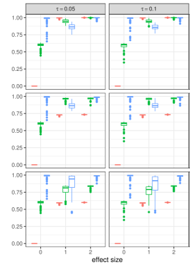
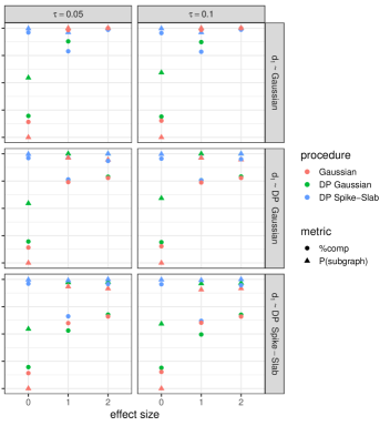
Figure 3: The left two columns display the average posterior probability of true pairwise treatment comparisons. The right two columns display results from applying the method described in Section 3 to summarize 15 treatments in the simulation study. The triangle symbol corresponds to the average posterior probability associated with the estimated sub-graph. Circles correspond to the sparsity of the estimated sub-graph. The lower the value, the more sparse and the smaller number of comparisons.

6 Analysis of the Antidepressants Dataset

We now proceed to apply the DP Spike-Slab approach to the data described in Section 2.1. The Gaussian effects model is also fit to provide context. Each of the two models were fit by collecting 3000 total MCMC samples from three independent chains with disparate starting values. Each chain was thinned by 100 iterates after discarding the first 100,000 iterates as burn-in. For both methods we set $m_{b}=0$, $s_{b}=10$, $m_{\ell}=-2.34$, and $s_{\ell}=2$. The later two hyperprior values are recommended in Turner et al., (2012). For the DP Spike-Slab model we also set $a_{\omega}=b_{\omega}=1$, $\alpha=1$, and $v_{0}=0.1$.

For the DP Spike-Slab approach, $d_{1k}$ can be exactly equal to 0 or $d_{1k^{\prime}}$. For this reason, achieving an credible interval of arbitrary posterior probability level might not be possible, and the construction of credible intervals requires special attention (see Section 4.3 of Womack et al., 2014). We summarize the posterior distribution of treatment effects using $p_{j=k}$, $p_{j>k}$, and $p_{j<k}$, which were introduced in Section 3. In particular, we use the following criteria that produces a conditional type of a $(1-\alpha)$ credible interval. Let $o_{kk^{\prime}}=\exp(d_{1k^{\prime}}-d_{1k})$ denote the odds ratio of treatment $k$ compared to treatment $k^{\prime}$. Then, using a strategy that resembles that in Womack et al., (2014), we define a $(1-\alpha)$-conditional credible interval as

$${\rm CI}(o_{jk})=\left\{\begin{array}[]{cl}\{1\}&\mbox{if }p_{j=k}=p(j,k);\\ \left[{\rm quantile}_{1-(1-\alpha/2)p_{j>k}}(o_{jk}),{\rm quantile}_{1-(\alpha/2)p_{j>k}}(o_{jk})\right]&\mbox{if }p_{j>k}=p(i,j);\\ \left[{\rm quantile}_{(\alpha/2)p_{j<k}}(o_{jk}),{\rm quantile}_{(1-\alpha/2)p_{j<k}}(o_{jk})\right]&\mbox{if }p_{j<k}=p(i,j).\end{array}\right.$$

We then report ${\rm CI}(o_{jk})$ along with $\Pr(o_{jk}\in{\rm CI}(o_{jk})|{\rm Data})$, where

$$\Pr(o_{jk}<{\rm quantile}_{a}(o_{jk})|{\rm Data})=a.$$

Notice that if $p_{j>k}=1$ or $p_{j<k}=1$ then $\Pr(o_{jk}\in{\rm CI}(o_{jk})|{\rm Data})=(1-\alpha)$.

Figures 4 and 5 display the posterior network treatment effects based on the Gaussian effects and DP Spike-Slab models, respectively. The graphs’ interpretations are detailed in Section 3 (Figure 2). The conventional Gaussian effects model was not able to identify the relationships of exactly the same treatment performance, so all treatment relationships in the graphs in Figure 4 were visualized as one-directional arrows. Based on the cumulative probabilities of being among the four most efficacious treatments, the original study of Cipriani et al., (2009) concluded that the best treatments were mirtazapine (24.4%), escitalopram (23.7%), venlafaxine (22.3%), sertraline (20.3%), citalopram (3.4%), milnacipran (2.7%), bupropion (2.0%), duloxetine (0.9%), fluvoxamine (0.7%), paroxetine (0.1%), fluoxetine (0.0%), and reboxetine (0.0%), i.e., treatments 8, 4, 12, 11, 2, 7, 1, 3, 6, 9, 5, and 10, accordingly. Treatments 8, 4, 12, and 11 seem to be in a cluster of best treatments because their cumulative probabilities were all about 20% to 25% and noticeably larger than the remaining treatments.

Our re-analyses based on the Gaussian effects model were generally consistent with these original findings, while there were a few exceptions. Specifically, in Figure 4(a), the full relationships between all 66 treatment comparisons indicate that treatment 4 was the best, followed by treatments 12, 11, 8, 2, 3, 7, 1, 9, 5, 6, and 10, accordingly. These differences in the rankings from the original conclusions were not surprising; the cumulative probabilities for treatment rankings in the original analyses were fairly similar, and some differences could be due to Monte Carlo sampling errors when performing the Bayesian analyses. Without trimming any treatment comparisons, the foregoing exact relationships between all treatment comparisons occurred only with a posterior joint probability of $<$0.01. This further suggested that these relationships may not be reliable for practical applications.

(a) $\Pr(\mathcal{E}=\mbox{mode graph}|{\rm Data})<0.01$

(b) $\Pr(\mathcal{E}=E_{\gamma}|{\rm Data})<0.01$, $\gamma=0.33$

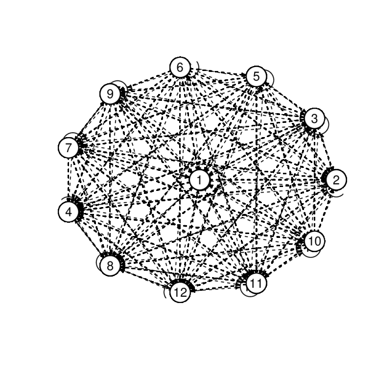
(c) $\Pr(\mathcal{E}=E_{\gamma}|{\rm Data})=0.59$, $\gamma=0.88$

(d) $\Pr(\mathcal{E}=E_{\gamma}|{\rm Data})=0.77$, $\gamma=0.96$

(e) $\Pr(\mathcal{E}=E_{\gamma}|{\rm Data})=0.89$, $\gamma=0.98$

(f) $\Pr(\mathcal{E}=E_{\gamma}|{\rm Data})=0.97$, $\gamma=0.99$

Figure 4: Posterior network treatment effects based on the Gaussian effects model. A dashed one-directional arrow from A to B indicates that treatment B performs better treatment A. A solid bi-directional arrow between A and B indicates that treatments A and B have the same performance.

(a) $\Pr(\mathcal{E}=\mbox{mode graph}|{\rm Data})=0.36$

(b) $\Pr(\mathcal{E}=E_{\gamma}|{\rm Data})=0.36$, $\gamma=0.33$

(c) $\Pr(\mathcal{E}=E_{\gamma}|{\rm Data})=0.57$, $\gamma=0.84$

(d) $\Pr(\mathcal{E}=E_{\gamma}|{\rm Data})=0.78$, $\gamma=0.88$

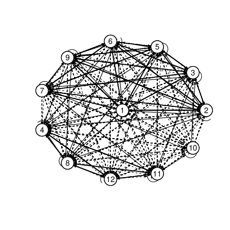
(e) $\Pr(\mathcal{E}=E_{\gamma}|{\rm Data})=0.82$, $\gamma=0.93$

(f) $\Pr(\mathcal{E}=E_{\gamma}|{\rm Data})=0.96$, $\gamma=0.97$

Figure 5: Posterior network treatment effects based on the DP Spike-Slab model. A dashed one-directional arrow from A to B indicates that treatment B performs better treatment A. A solid bi-directional arrow between A and B indicates that treatments A and B have the same performance.

Figures 4(b)–4(f) present the network treatment effects after trimming some uncertain treatment comparisons so that the $\tilde{p}(j,k)$’s defined in Section 3 are beyond a specific threshold $\gamma$ for all comparisons $j$ vs. $k$ connected with arrows. For example, if we require $\gamma=0.96$, the number of eligible treatment comparisons was reduced to 34, and the posterior joint probability of the network relationships became 0.77 (Figure 4(d)). The cluster of best treatments, 8, 4, 12, and 11, identified in the original analyses were no longer connected with arrows, so their relationships became uncertain under the restriction of $\gamma$. If we increased $\gamma$ to 0.98, then the posterior joint probability increased to 0.89 (Figure 4(e)). If the threshold was further increased to 0.99, then the posterior joint probability became 0.97 (Figure 4(f)). Such a high joint probability could generally ensure the reliability of treatment comparisons. For example, in this case, we could conclude that treatments 8 was better than treatments 3, 5, 6, 9, and 10, treatment 4 was better than treatments 3, 5, 9, and 10, and each of treatments 11 and 12 was better than treatments 5, 9, and 10. No reliable conclusion could be drawn about treatment 7.

Using our proposed DP Spike-Slab model, we were able to identify treatments with exactly the same performance. Without trimming any uncertain treatment comparisons, Figure 5(a) shows the full network relationships. Treatments 4, 8, 11, and 12 were formally identified to have the same performance, supporting the previous observation based on the original analyses. Their performance was better than treatments 1, 2, 3, 5, 6, 7, and 9, which also had the same performance. Treatment 10 had the worst performance. However, the posterior joint probability of these network relationships was only 0.36. As in the analyses using the Gaussian effects model, we increased the threshold $\gamma$ to achieve more satisfactory joint probabilities. If the threshold was set to 0.93, the posterior joint probability became 0.82. We conclude that treatments 4, 8, and 12 had the same best treatment. Treatment 11 was no longer in this cluster; nevertheless, it was better than treatment 10. In addition, treatments 3, 5, 6, and 9 have the same performance, and they were worse than the group of treatments 4, 8, and 12. We could not draw reliable conclusions about treatments 1, 2, and 7. If the threshold was further set to 0.97, the posterior joint probability increased to 0.96. In this case, we could only reliably conclude that treatments 3, 5, and 9 had the same performance, and treatment 4 was better than 10. No reliable conclusions could be drawn for other treatment comparisons.

Table 1 gives the league table of results for all treatment comparisons based on both the Gaussian effects and DP Spike-Slab models. For the DP Spike-Slab model, the league table reports the posterior probability of treatments being equal for each comparison and the posterior probability of treatment effect belonging to the interval estimate. For the conventional Gaussian effects model, because it could not model the cases of exact equal treatment effects, the posterior probability of treatments being equal was always 0, and the posterior probability of treatment effect belonging to the interval estimate was always 95%. The posterior mean estimates of odds ratios by the DP Spike-Slab model were generally similar to those by the Gaussian effects model, while there were still some noticeable differences. The interval estimates by the two models were substantially different for most comparisons. For example, the odds ratio of treatment 2 vs. 1 was estimated as 1.03 by the Gaussian effects model and as 1.04 by DP Spike-Slab; both estimates were close to the null value of 1. Nevertheless, the Gaussian effects model could not conclude that the odds ratio was exactly 1; it could only give a 95% credible interval of [0.84, 1.26]. On the other hand, the credible interval by the DP Spike-Slab model was [1.00, 1.00], and the posterior probability of the odds ratio equal 1 was 74.57%. For another comparison, treatment 8 vs. 7, the Gaussian effects model gave a posterior mean odds ratio of 1.37 with 95% credible interval [0.99, 1.84], covering 1. DP Spike-Slab gave an estimate of 1.23, with a probability of 20.13% that these two treatments have exactly the same effect. The interval estimate was [1.17, 1.39], and the posterior probability of treatment effect belonging to this interval was 76.53%.

Table 1: League table of the network meta-analysis of antidepressants. The upper triangular cells are produced by the Gaussian effects model, the lower triangular cells are produced by the DP Spike-Slab model, and the diagonal cells present the treatment names. Each data cell includes the posterior mean estimate of the odds ratio (the treatment in the later alphabetical order vs. that in the former alphabetical order), with 95% credible intervals in parentheses. For the DP Spike-Slab model, we report intervals estimated using method as described in Section 6; in each cell, we also report the posterior probability of treatments being equal in parentheses in the first line and that of treatment effect belonging to the reported interval in the last line.

7 Discussion

This article has proposed a novel nonparametric Bayesian approach for NMA. The approach overcomes several limitations of existing NMA, including failure to account for uncertainties in treatment rankings. By employing a spike and slab distribution, the treatment ordering statement of our Bayesian approach can model the cases of exactly equal treatment effects (i.e., treatments with the same rank). The approach can also yield posterior network treatment effects showing the relationships among treatments and the corresponding posterior joint probability of having such relationships. This framework is entirely different from the current practice of interpreting each pair of treatment comparisons separately, which could lead to exaggerated treatment effects caused by multiplicity issues. The simulation study showed that our method is able to accurately recover treatment rankings when equal treatment effects are present in an NMA. In addition, it also showed that this added flexibility comes at a limited cost when equal treatments do not exist, and conventional NMA methods have no hope of producing accurate treatment rankings when there exist treatments whose effects are essentially the same.

Nevertheless, this paper has some limitations. First, we only considered NMAs with binary outcomes. The proposed methods could be broadly generalized to other types of outcomes (e.g., continuous or survival), and more efforts are needed to generalize them (Dias et al.,, 2013). Second, the methods are developed under the assumption of evidence consistency, i.e., direct comparisons share the same overall effects as indirect comparisons. However, this might not be valid in some cases; for example, some comparisons could be contaminated by outliers, or some effect modifiers should be incorporated in a network meta-regression (Higgins et al.,, 2012; Jansen and Naci,, 2013). The proposed methods could be potentially extended to deal with inconsistency. For example, inconsistency is generally modeled via introducing additional parameters in an NMA model, either as treatment-loop-specific parameters or design-by-treatment interactions (Bucher et al.,, 1997; Chaimani et al.,, 2017). These inconsistency parameters may dramatically increase model complexity and thus lead to treatment effect estimates with larger variations. Nevertheless, inconsistency may actually exist in a few loops or design-by-treatment interactions for real-world data, and most inconsistency parameters are truly 0. The nonparametric Bayesian approach with the spike and slab distribution could be similarly used to permit inconsistency parameters being exactly estimated as 0. Third, the induced random partition model from a DP can be restrictive. New approaches may be developed to allow incorporating prior information on partition probabilities. For example, it might prove useful to include information regarding treatment composition and/or clinicians’ expertise in the partition model.

References

- Barrientos et al., (2021) Barrientos, A. F., Sen, D., Page, G. L., and Dunson, D. B. (2021). Bayesian inferences on uncertain ranks and orderings: Application to ranking players and lineups. arXiv:1907.04842.
- Bucher et al., (1997) Bucher, H. C., Guyatt, G. H., Griffith, L. E., and Walter, S. D. (1997). The results of direct and indirect treatment comparisons in meta-analysis of randomized controlled trials. Journal of Clinical Epidemiology, 50(6):683–691.
- Canale et al., (2017) Canale, A., Lijoi, A., Nipoti, B., and Prünster, I. (2017). On the Pitman–Yor process with spike and slab base measure. Biometrika, 104(3):681–697.
- Chaimani et al., (2017) Chaimani, A., Salanti, G., Leucht, S., Geddes, J. R., and Cipriani, A. (2017). Common pitfalls and mistakes in the set-up, analysis and interpretation of results in network meta-analysis: what clinicians should look for in a published article. Evidence-Based Mental Health, 20(3):88–94.
- Cipriani et al., (2009) Cipriani, A., Furukawa, T. A., Salanti, G., Geddes, J. R., Higgins, J. P. T., Churchill, R., Watanabe, N., Nakagawa, A., Omori, I. M., McGuire, H., Tansella, M., and Barbui, C. (2009). Comparative efficacy and acceptability of 12 new-generation antidepressants: a multiple-treatments meta-analysis. The Lancet, 373(9665):746–758.
- Cipriani et al., (2013) Cipriani, A., Higgins, J. P. T., Geddes, J. R., and Salanti, G. (2013). Conceptual and technical challenges in network meta-analysis. Annals of Internal Medicine, 159(2):130–137.
- Dias and Ades, (2016) Dias, S. and Ades, A. E. (2016). Absolute or relative effects? Arm-based synthesis of trial data. Research Synthesis Methods, 7(1):23–28.
- Dias et al., (2013) Dias, S., Sutton, A. J., Ades, A. E., and Welton, N. J. (2013). Evidence synthesis for decision making 2: a generalized linear modeling framework for pairwise and network meta-analysis of randomized controlled trials. Medical Decision Making, 33(5):607–617.
- Efthimiou et al., (2016) Efthimiou, O., Debray, T. P., van Valkenhoef, G., Trelle, S., Panayidou, K., Moons, K. G., Reitsma, J. B., Shang, A., and Salanti, G. (2016). GetReal in network meta-analysis: a review of the methodology. Research Synthesis Methods, 7(3):236–263.
- Efthimiou and White, (2020) Efthimiou, O. and White, I. R. (2020). The dark side of the force: multiplicity issues in network meta-analysis and how to address them. Research Synthesis Methods, 11(1):105–122.
- Gelman et al., (2014) Gelman, A., Carlin, J. B., Stern, H. S., Dunson, D. B., Vehtari, A., and Rubin, D. B. (2014). Bayesian Data Analysis. Chapman & Hall/CRC Texts in Statistical Science. CRC Press, Boca Raton, FL, 3rd edition.
- George and McCulloch, (1993) George, E. I. and McCulloch, R. E. (1993). Variable selection via Gibbs sampling. Journal of the American Statistical Association, 88(423):881–889.
- Ghosal and van der Vaart, (2017) Ghosal, S. and van der Vaart, A. (2017). Fundamentals of Nonparametric Bayesian Inference. Cambridge Series in Statistical and Probabilistic Mathematics. Cambridge University Press.
- Higgins et al., (2012) Higgins, J. P. T., Jackson, D., Barrett, J. K., Lu, G., Ades, A. E., and White, I. R. (2012). Consistency and inconsistency in network meta-analysis: concepts and models for multi-arm studies. Research Synthesis Methods, 3(2):98–110.
- Higgins and Welton, (2015) Higgins, J. P. T. and Welton, N. J. (2015). Network meta-analysis: a norm for comparative effectiveness? The Lancet, 386(9994):628–630.
- Higgins and Whitehead, (1996) Higgins, J. P. T. and Whitehead, A. (1996). Borrowing strength from external trials in a meta-analysis. Statistics in Medicine, 15(24):2733–2749.
- Hong et al., (2016) Hong, H., Chu, H., Zhang, J., and Carlin, B. P. (2016). Rejoinder to the discussion of “a Bayesian missing data framework for generalized multiple outcome mixed treatment comparisons,” by S. Dias and AE Ades. Research Synthesis Methods, 7(1):29–33.
- Hutton et al., (2015) Hutton, B., Salanti, G., Caldwell, D. M., Chaimani, A., Schmid, C. H., Cameron, C., Ioannidis, J. P. A., Straus, S., Thorlund, K., Jansen, J. P., Mulrow, C., Catalá-López, F., Gøtzsche, P. C., Dickersin, K., Boutron, I., and Altman, D. G. (2015). The PRISMA extension statement for reporting of systematic reviews incorporating network meta-analyses of health care interventions: checklist and explanations. Annals of Internal Medicine, 162(11):777–784.
- Ishwaran and James, (2001) Ishwaran, H. and James, L. F. (2001). Gibbs sampling methods for stick-breaking priors. Journal of the American Statistical Association, 96(453):161–173.
- Ishwaran and Rao, (2005) Ishwaran, H. and Rao, J. S. (2005). Spike and slab variable selection: Frequentist and bayesian strategies. The Annals of Statistics, 33(2):730–773.
- Jackson et al., (2017) Jackson, D., White, I. R., Price, M., Copas, J., and Riley, R. D. (2017). Borrowing of strength and study weights in multivariate and network meta-analysis. Statistical Methods in Medical Research, 26(6):2853–2868.
- Jansen and Naci, (2013) Jansen, J. P. and Naci, H. (2013). Is network meta-analysis as valid as standard pairwise meta-analysis? It all depends on the distribution of effect modifiers. BMC Medicine, 11:159.
- Johnson and Rossell, (2010) Johnson, V. E. and Rossell, D. (2010). On the use of non-local prior densities in Bayesian hypothesis tests. Journal of the Royal Statistical Society Series B, 72:143–170.
- Kim et al., (2009) Kim, S., Dahl, D. B., and Vannucci, M. (2009). Spiked Dirichlet process prior for Bayesian multiple hypothesis testing in random effects models. Bayesian Analysis, 4:707–732.
- Lin et al., (2019) Lin, L., Xing, A., Kofler, M. J., and Murad, M. H. (2019). Borrowing of strength from indirect evidence in 40 network meta-analyses. Journal of Clinical Epidemiology, 106:41–49.
- Lin et al., (2017) Lin, L., Zhang, J., Hodges, J. S., and Chu, H. (2017). Performing arm-based network meta-analysis in R with the pcnetmeta package. Journal of Statistical Software, 80:5.
- Lu and Ades, (2004) Lu, G. and Ades, A. E. (2004). Combination of direct and indirect evidence in mixed treatment comparisons. Statistics in Medicine, 23(20):3105–3124.
- Lu and Ades, (2006) Lu, G. and Ades, A. E. (2006). Assessing evidence inconsistency in mixed treatment comparisons. Journal of the American Statistical Association, 101:447–459.
- Lumley, (2002) Lumley, T. (2002). Network meta-analysis for indirect treatment comparisons. Statistics in Medicine, 21(16):2313–2324.
- Magni et al., (2013) Magni, L. R., Purgato, M., Gastaldon, C., Papola, D., Furukawa, T. A., Cipriani, A., and Barbui, C. (2013). Fluoxetine versus other types of pharmacotherapy for depression. Cochrane Database of Systematic Reviews, 7:Art. No.: CD004185.
- Malsiner-Walli and Wagner, (2011) Malsiner-Walli, G. and Wagner, H. (2011). Comparing spike and slab priors for Bayesian variable selection. Austrian Journal of Statistics, 40(4):241–264.
- Mavridis et al., (2020) Mavridis, D., Porcher, R., Nikolakopoulou, A., Salanti, G., and Ravaud, P. (2020). Extensions of the probabilistic ranking metrics of competing treatments in network meta-analysis to reflect clinically important relative differences on many outcomes. Biometrical Journal, 62(2):375–385.
- Mills et al., (2013) Mills, E. J., Thorlund, K., and Ioannidis, J. P. A. (2013). Demystifying trial networks and network meta-analysis. BMJ, 346:f2914.
- Mitchell and Beauchamp, (1988) Mitchell, T. J. and Beauchamp, J. J. (1988). Bayesian variable selection in linear regression. Journal of the American Statistical Association, 83:1023–1036.
- Müller et al., (2015) Müller, P., Quintana, F. A., Jara, A., and Hanson, T., editors (2015). Bayesian Nonparametric Data Analysis. Springer International Publishing, Switzerland, 1 edition.
- Petropoulou et al., (2017) Petropoulou, M., Nikolakopoulou, A., Veroniki, A.-A., Rios, P., Vafaei, A., Zarin, W., Giannatsi, M., Sullivan, S., Tricco, A. C., Chaimani, A., Egger, M., and Salanti, G. (2017). Bibliographic study showed improving statistical methodology of network meta-analyses published between 1999 and 2015. Journal of Clinical Epidemiology, 82:20–28.
- Riley et al., (2017) Riley, R. D., Jackson, D., Salanti, G., Burke, D. L., Price, M., Kirkham, J., and White, I. R. (2017). Multivariate and network meta-analysis of multiple outcomes and multiple treatments: rationale, concepts, and examples. BMJ, 358:j3932.
- Rosenberger et al., (2021) Rosenberger, K. J., Duan, R., Chen, Y., and Lin, L. (2021). Predictive P-score for treatment ranking in bayesian network meta-analysis. BMC Medical Research Methodology, 21:213.
- Rücker and Schwarzer, (2015) Rücker, G. and Schwarzer, G. (2015). Ranking treatments in frequentist network meta-analysis works without resampling methods. BMC Medical Research Methodology, 15:58.
- Rücker and Schwarzer, (2017) Rücker, G. and Schwarzer, G. (2017). Resolve conflicting rankings of outcomes in network meta-analysis: partial ordering of treatments. Research Synthesis Methods, 8(4):526–536.
- Salanti, (2012) Salanti, G. (2012). Indirect and mixed-treatment comparison, network, or multiple-treatments meta-analysis: many names, many benefits, many concerns for the next generation evidence synthesis tool. Research Synthesis Methods, 3(2):80–97.
- Salanti et al., (2011) Salanti, G., Ades, A. E., and Ioannidis, J. P. A. (2011). Graphical methods and numerical summaries for presenting results from multiple-treatment meta-analysis: an overview and tutorial. Journal of Clinical Epidemiology, 64(2):163–171.
- Scarpa and Dunson, (2009) Scarpa, B. and Dunson, D. B. (2009). Bayesian hierarchical functional data analysis via contaminated informative priors. Biometrics, 65:772–780.
- Sethuraman, (1994) Sethuraman, J. (1994). A constructive definition of Dirichlet priors. Statistica Sinica, 4:639–650.
- Trinquart et al., (2016) Trinquart, L., Attiche, N., Bafeta, A., Porcher, R., and Ravaud, P. (2016). Uncertainty in treatment rankings: reanalysis of network meta-analyses of randomized trials. Annals of Internal Medicine, 164(10):666–673.
- Turner et al., (2012) Turner, R. M., Davey, J., Clarke, M. J., Thompson, S. G., and Higgins, J. P. T. (2012). Predicting the extent of heterogeneity in meta-analysis, using empirical data from the Cochrane Database of Systemic Reviews. International Journal of Epidemiology, 41:818–827.
- Veroniki et al., (2018) Veroniki, A. A., Straus, S. E., Rücker, G., and Tricco, A. C. (2018). Is providing uncertainty intervals in treatment ranking helpful in a network meta-analysis? Journal of Clinical Epidemiology, 100:122–129.
- White et al., (2019) White, I. R., Turner, R. M., Karahalios, A., and Salanti, G. (2019). A comparison of arm-based and contrast-based models for network meta-analysis. Statistics in Medicine, 38(27):5197–5213.
- Womack et al., (2014) Womack, A. J., León-Novelo, L., and Casella, G. (2014). Inference from intrinsic bayes’ procedures under model selection and uncertainty. Journal of the American Statistical Association, 109(507):1040–1053.
- Wu et al., (2021) Wu, Y.-C., Shih, M.-C., and Tu, Y.-K. (2021). Using normalized entropy to measure uncertainty of rankings for network meta-analyses. Medical Decision Making, 41(6):706–713.
- Zhang et al., (2014) Zhang, J., Carlin, B. P., Neaton, J. D., Soon, G. G., Nie, L., Kane, R., Virnig, B. A., and Chu, H. (2014). Network meta-analysis of randomized clinical trials: reporting the proper summaries. Clinical Trials, 11(2):246–262.