High-fidelity intensity diffraction tomography with a non-paraxial multiple-scattering model

Abstract

We propose a novel intensity diffraction tomography (IDT) reconstruction algorithm based on the split-step non-paraxial (SSNP) model for recovering the 3D refractive index (RI) distribution of multiple-scattering biological samples. High-quality IDT reconstruction requires high-angle illumination to encode both low- and high- spatial frequency information of the 3D biological sample. We show that our SSNP model can more accurately compute multiple scattering from high-angle illumination compared to paraxial approximation-based multiple-scattering models. We apply this SSNP model to both sequential and multiplexed IDT techniques. We develop a unified reconstruction algorithm for both IDT modalities that is highly computationally efficient and is implemented by a modular automatic differentiation framework. We demonstrate the capability of our reconstruction algorithm on both weakly scattering buccal epithelial cells and strongly scattering live C. elegans worms and live C. elegans embryos.

1 Introduction

3D quantitative phase imaging (QPI) has found use in many biological applications by providing 3D refractive index (RI) information of the samples [1]. Optical diffraction tomography (ODT) [2] is the most widely used technique for 3D QPI. It works by directly measuring the complex field using an interferometry setup from multiple angles and then recovering the 3D RI distribution with an inverse scattering model. However, the need for coherent illumination and an interferometric path complicates the system and makes it prone to speckle artifacts [3].

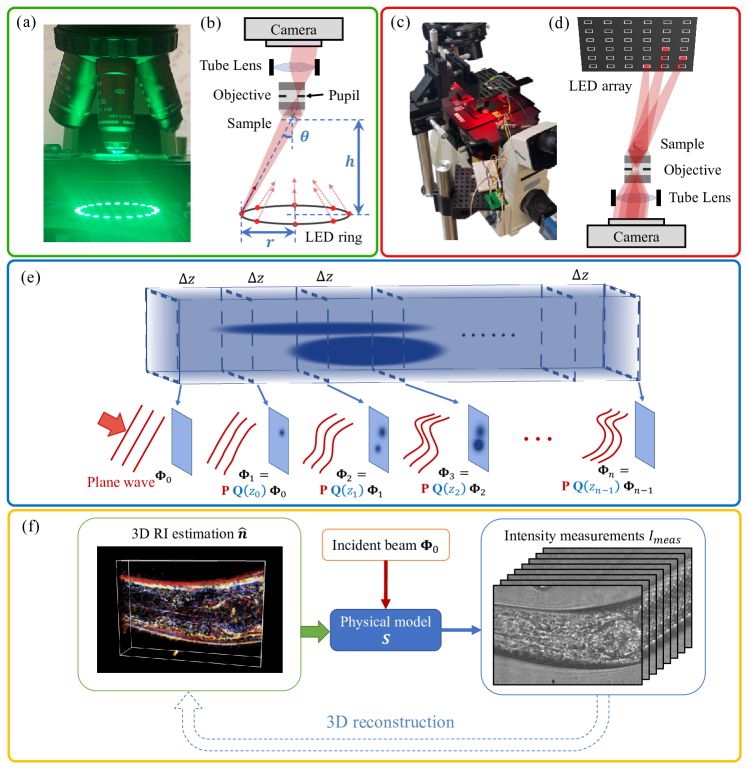
Figure 1: (a-b) Our annular IDT setup uses an LED ring of radius $r$ to illuminate the sample sequentially. The ring is placed $h$ away from the sample and the illumination angle $\theta=\arctan(r/h)$ matches the objective NA. (c-d) Our multiplexed IDT setup uses an LED matrix and illuminates the sample using several LEDs simultaneously. (e) The SSNP model involves successive propagation $\mathbf{P}$ and scattering $\mathbf{Q}$ operations to compute the scattered field and its axial derivative $\bm{\Phi}_{i}$ from one slice to the next. (f) 3D reconstruction by iteratively solving the SSNP-based optimization problem.

Intensity diffraction tomography (IDT) is an alternative 3D QPI technique that recovers 3D phase information from intensity-only measurements on a “non-interferometry” setup [4]. Recently, several groups have demonstrated that IDT can be easily implemented on a standard microscope using a programmable LED array [5, 6, 7, 8, 9, 10, 11, 12, 13]. Most of the IDT acquisition strategies require taking hundreds of images to achieve high-resolution 3D RI reconstruction. Recently, our group has developed two strategies to push the acquisition speed and enabled visualizing dynamic biological samples. The annular IDT achieved a $10\text{\,}\mathrm{Hz}$ volume rate by using an LED ring illuminator that provides illumination angles matching the objective’s numerical aperture (NA) [7]. The multiplexed IDT provided a $4-$10\text{\,}\mathrm{Hz}$$ acquisition rate by simultaneously tuning on multiple LEDs using the most widely used LED matrix [10].

The 3D reconstruction of IDT requires an inverse scattering model, similar to ODT. The single-scattering models are based on the first-Born [5, 7, 10] or first-Rytov [12] approximation, allowing closed-form solutions due to the linear relationship between the scattering potential and the measurements. However, the accuracy of these models are fundamentally limited by the weak scattering assumption. Recently, several multiple-scattering models have been developed based on the beam propagation method (BPM) [6, 14] and multi-layer Born (MLB) model [8] and showed enhanced resolution and fidelity on strongly scattering biological samples, such as C. elegans embryos and worm. However, the accuracy of the BPM degrades for high-NA systems since it relies on the paraxial approximation [15], which limits its effectiveness for high-resolution imaging using high-NA optics. The MLB model relies on the local weak scattering approximation within each layer, which limits the model fidelity for strongly scattering samples. Recently, a split-step non-paraxial (SSNP) multiple-scattering model has been developed for ODT [16], which demonstrated substantial improvement in reconstruction quality compared to the single-scattering and BPM methods. This ODT setup, however, needs a laser and a spatial light modulator to provide the coherent illumination and a interferometric path to retrieve the phase information of the light field. Besides, the large number of measurements used limits this system’s ability of high-speed imaging for dynamic samples. Inspired by this work, here we develop an SSNP IDT model for the two fast-acquisition IDT modalities. We demonstrate that our model can effectively provide high-quality 3D RI reconstruction on several biological samples with simple “non-interferometric” IDT setups.

The SSNP model is a wave propagation model derived from the Helmholtz equation [17]. Similar to the BPM and MLB, the SSNP works by axially splitting the sample into multiple slices and propagate the wave slice-wise. The BPM and MLB rely on local homogeneous RI and weak RI contrast, respectively, to decouple the diffraction from the local phase modulation / single scattering within each slice. Instead, the SSNP simultaneously propagates both the field and the axial derivative of the field so that the coupling between the diffraction and local phase modulation is modeled jointly without making assumptions about the local RI distribution [16]. Due to the same “multi-slice” structure as the BPM and MLB, together with the fast Fourier transform (FFT)-based propagation implementation [16], the SSNP incurs similar computational costs while providing improved fidelity on high-scattering biological samples.

Here we first extend the SSNP model to IDT and apply it to two IDT modalities, including the sequential and multiplexed IDT (as summarized in Fig. 1a-d). Next, we derive an efficient SSNP-IDT forward model (as illustrated in Fig. 1e). We then derive a reconstruction algorithm by solving a regularized least-squares optimization (Fig. 1f). We elucidate on how the analytical gradient of the SSNP-IDT model can be efficiently computed, akin to “back-propagation”. Furthermore, we devise a unified algorithmic framework that allows fast 3D recovery from both sequential and multiplexed IDT measurements based on a memory efficient automatic differentiation framework. To quantitatively evaluate the fidelity of the forward model and reconstruction algorithm, we conduct numerical simulations. Lastly, we experimentally demonstrate high-quality, large field-of-view (FOV) 3D RI reconstructions on buccal epithelial cells and a live C. elegans worm from annular IDT and live C. elegans embryos from multiplexed IDT.

2 Theory

2.1 SSNP theory

The SSNP model first discretizes the 3D sample into a series of axial ($z$) slices and then calculates the internal field slice-by-slice ($xy$), as illustrated in Fig. 1(e). In the following, we provide the key steps to derive the governing equations for light propagating through the sample by following [17, 16], and then describe the integration to specific IDT systems in separate sections.

The scalar wave propagation in an inhomogeneous medium with a 3D RI distribution $n(\bm{r})$ satisfies the Helmholtz equation

$$\left(\frac{\partial^{2}}{\partial x^{2}}+\frac{\partial^{2}}{\partial y^{2}}+\frac{\partial^{2}}{\partial z^{2}}\right)\,\varphi(\bm{r})+\,k_{0}^{2}\;n^{2}(\bm{r})\,\varphi(\bm{r})=0,$$ (1)

where $\bm{r}=(x,y,z)$ denotes the 3D spatial position, $\varphi$ is the field and $k_{0}=2\pi/\lambda$ is the wavenumber in free space. We derive the SSNP model by first rewriting Eq. (1) into a matrix form

$$\diffp{\bm{\Phi}(\bm{r})}z=\bm{\mathrm{H}}(\bm{r})\;\bm{\Phi}(\bm{r}),$$ (2)

where

$$\bm{\Phi}(\bm{r})=\begin{pmatrix}\varphi(\bm{r})\\ \frac{\partial\varphi}{\partial z}\end{pmatrix},\ \mathbf{H}(\bm{r})=\begin{pmatrix}0&1\\ -\diffp[2]{}x-\diffp[2]{}y-\,k_{0}^{2}n^{2}(\bm{r})\!\!&0\end{pmatrix}.$$ (3)

Here the vector $\bm{\Phi}(\bm{r})$ contains both the field itself and its $z$-derivative, which is the quantity of interest in the SSNP-based wave propagation. For brevity, we will refer $\bm{\Phi}$ to the 2D “field” at a slice in the rest of this article. Next, we decompose the operator $\bm{\mathrm{H}}(\bm{r})=\mathbf{H}_{1}+\mathbf{H}_{2}(\bm{r})$, which decouples the diffraction operator $\bm{\mathrm{H}}_{1}$ and the scattering operator $\bm{\mathrm{H}}_{2}(\bm{r})$:

$$\mathbf{H}_{1}=\begin{pmatrix}0&1\\ -\diffp[2]{}x-\diffp[2]{}y\!-\!\,k_{0}^{2}n_{0}^{2}\!&0\end{pmatrix},\,\mathbf{H}_{2}(\bm{r})=\begin{pmatrix}0&0\\ k_{0}^{2}(n_{0}^{2}-n^{2}(\bm{r}))\!&0\end{pmatrix}.$$ (4)

Here $n_{0}$ is the RI of the background medium. $\bm{\mathrm{H}}_{1}$ is spatially invariant describing the diffraction in the homogeneous background medium. $\bm{\mathrm{H}}_{2}(\bm{r})$ is spatially variant based on the distribution of the scattering potential $\propto(n_{0}^{2}-n^{2}(\bm{r}))$, akin to the Born scattering model. Equations (2)–(4) constitute the governing equations in the SSNP model.

Next, we describe the numerical method to efficiently calculate Eq. (2)–(4). First, we discretize the sample volume as a series of $z$-slices. Second, to compute the field propagating a small distance $\Delta z$ between two adjacent slices, we approximate Eq. (2) as a first-order homogeneous linear system of differential equations with constant coefficients. The solution is approximated as

$$\bm{\Phi}_{xy}(z+\Delta z)\approx\exp(\mathbf{H}(\bm{r})\Delta z)\,\bm{\Phi}_{xy}(z)\approx\mathbf{P}\,\mathbf{Q}(z)\,\bm{\Phi}_{xy}(z),$$ (5)

where $\bm{\Phi}_{xy}(z)$ represents the 2D field at the axial position $z$, and

$$\mathbf{P}=\exp(\mathbf{H}_{1}\Delta z),\ \mathbf{Q}(z)=\exp(\mathbf{H}_{2}(x,y,z)\Delta z).$$ (6)

The operator $\mathbf{P}$ computes the propagation by $\Delta z$ in the homogeneous background medium and can be efficiently computed by FFT as

$$\mathbf{P}\,\bm{\Phi}_{xy} =\mathcal{F}_{xy}^{-1}\{\widetilde{\mathbf{P}}\,\mathcal{F}_{xy}\{\bm{\Phi}_{xy}\}\}$$

$$=\mathcal{F}_{xy}^{-1}\left\{\begin{pmatrix}\cos(k_{z}\Delta z)&\sin(k_{z}\Delta z)/k_{z}\\ -k_{z}\sin(k_{z}\Delta z)\!&\cos(k_{z}\Delta z)\end{pmatrix}\mathcal{F}_{xy}\{\bm{\Phi}_{xy}\}\right\},$$ (7)

where $\mathcal{F}_{xy}\{\cdot\}$ and $\mathcal{F}_{xy}^{-1}\{\cdot\}$ denote the 2D Fourier and inverse Fourier transform on the XY plane, respectively, and $k_{x}$ and $k_{y}$ are the corresponding $\mathbf{k}$ (wave vector) components. $k_{z}=\sqrt{k_{0}^{2}\,n_{0}^{2}-k_{x}^{2}-k_{y}^{2}}$ if $k_{x}^{2}+k_{y}^{2}\leq k_{0}^{2}\,n_{0}^{2}$; otherwise, $\widetilde{\mathbf{P}}=\bm{0}$ that removes the evanescent component.

The operator $\mathbf{Q}(z)$ computes the scattering induced by the RI difference in the object slice at $z$ and is computed directly in the real space as

$$\mathbf{Q}(z)\,\bm{\Phi}_{xy}=\begin{pmatrix}1&0\\ k_{0}^{2}\left(n_{0}^{2}-n_{xy}^{2}(z)\right)\Delta z&1\end{pmatrix}\bm{\Phi}_{xy}.$$ (8)

The SSNP model computes the exit field at slice $z_{n}$ by recursively applying $\mathbf{P}$ and $\mathbf{Q}$ slice-wise starting from the illumination field, as illustrated in Fig. 1(e). Detailed derivations for Eq. (5)–(8) are provided in Supplement 1.

2.2 SSNP-based sequential IDT forward model

The sequential IDT, such as annular IDT [7], uses a single LED to illuminate the sample in each measurement. To derive the SSNP-based forward model, we first compute the illumination field and its axial derivative at $z=z_{0}$ as the initial condition to the SSNP equations. Each illumination field is a plane wave $\varphi(\bm{r})=\varphi_{0}\exp[j(k_{x}^{in}\,x+k_{y}^{in}\,y+k_{z}^{in}\,z)]$ where $\bm{k}^{in}=(k_{x}^{in},k_{y}^{in},k_{z}^{in})$ is the wave vector. By omitting the constant factors $\varphi_{0}$ and $\exp(j\,k_{z}^{in}\,z_{0})$, we have

$$\bm{\Phi}_{0}=\exp[j(k_{x}^{in}\,x+k_{y}^{in}\,y)]\ \begin{pmatrix}1\\ j\,k_{z}^{in}\end{pmatrix}.$$ (9)

For non-plane wave illumination, Supplement 1 provides a general treatment to construct $\bm{\Phi}_{0}$.

By propagating the illumination field through the sample with the SSNP equations, we obtain the exit field from the sample at plane $z_{n}$. To compute the field through the microscope reaching the camera $\bm{\Phi}_{\mathrm{cam}}$, we first back-propagate the exit field from $z_{n}$ to the front focal plane ($z_{\mathrm{focal}}$), and then filter it by the microscope’s pupil function:

$$\bm{\Phi}_{\mathrm{cam}}=\mathcal{P}_{\mathrm{NA}}\mathbf{P}_{\Delta z_{f}}\bm{\Phi}_{xy}(z_{n}),$$ (10)

where $\mathbf{P}_{\Delta z_{f}}=\exp(\mathbf{H}_{1}\Delta z_{f})$ is the propagation operator by a distance $\Delta z_{f}=z_{\mathrm{focal}}-z_{n}$. $\mathcal{P}_{\mathrm{NA}}$ denotes the low-pass filtering by the pupil function, and can be computed efficiently in the Fourier space as a multiplication between the pupil function $\widetilde{\mathcal{P}_{\mathrm{NA}}}$ and the Fourier transform of the back-propagated field (and its axial derivative). In our implementation, we assume a binary pupil function with a cutoff frequency at $k_{0}n_{0}\mathrm{NA}$ and ignore the apodization and aberrations. The field $\bm{\Phi}_{\mathrm{cam}}$ contains both forward-propagating and back-propagating components. In practice, the back-propagating component will introduce high-frequency artifacts [16], we extract only the forward-propagating component from $\bm{\Phi}_{\mathrm{cam}}$ by an operator $\operatorname{F}$. The forward-propagating field component at the camera plane $\varphi_{\mathrm{out}}$ is

$$\varphi_{\mathrm{out}} =\operatorname{F}\bm{\Phi}_{\mathrm{cam}}=\mathcal{F}_{xy}^{-1}\left\{\left(\mathcal{F}_{xy}\left\{\varphi_{\mathrm{cam}}\right\}-\frac{j}{k_{z}}\mathcal{F}_{xy}\left\{\diffp{\varphi_{\mathrm{cam}}}z\right\}\right)\middle/2\,\right\}$$

$$=\mathcal{F}_{xy}^{-1}\left\{\left(\frac{1}{2},\ -\frac{j}{2k_{z}}\right)\mathcal{F}_{xy}\{\bm{\Phi}_{\mathrm{cam}}\}\right\}.$$ (11)

Detailed derivation of $\operatorname{F}$ and a discussion about the bi-directional property of the SSNP model are provided in Supplement 1. Finally, the intensity from sequential IDT estimated by the SSNP model is $I_{\mathrm{out}}=\left|\varphi_{\mathrm{out}}\right|^{2}$.

To summarize, our SSNP-based sequential IDT (SSNP-sIDT) forward model can be written in the following compact form

$$I_{\mathrm{out}}=\left|\operatorname{F}\mathcal{P}_{\mathrm{NA}}\mathbf{P}_{\Delta z_{f}}\mathbf{P}\mathbf{Q}(z_{n-1})\ldots\mathbf{P}\mathbf{Q}(z_{1})\mathbf{P}\mathbf{Q}(z_{0})\bm{\Phi}_{xy}(z_{0})\right|^{2}.$$ (12)

2.3 SSNP-based multiplexed IDT forward model

Multiplexed IDT uses several LEDs to illuminate the sample in each measurement [10]. Since the light from different LEDs are incoherent with each other, we can model the scattering process independently and compute the measured intensity as the sum of the intensities from all the LEDs in each measurement. Therefore, the forward model of the SSNP-based multiplexed IDT (SSNP-mIDT) is similar to the sequential IDT but with an additional incoherent sum over Eq. (12):

$$I_{\mathrm{out}}=\sum_{m=1}^{M}I_{\mathrm{out}}^{m},$$ (13)

where $I_{\mathrm{out}}^{m}$ is the intensity from the $m$th LED. Each multiplexed measurement uses $M$ LEDs.

2.4 Inverse problem for SSNP-sIDT

Next, we formulate the inverse problem for reconstructing the 3D RI distribution using multiple intensity measurements taken from $L$ different LEDs $I_{\mathrm{meas}}^{l}$ indexed by $l=1,2,\dots,L$. We formulate the sequential IDT reconstruction as the following optimization problem

$$\hat{n}=\underset{n\in\Theta}{\operatorname{argmin}}\left\{\sum_{l=1}^{L}\left\lVert\sqrt{I_{\mathrm{out}}^{l}}-\sqrt{I_{\mathrm{meas}}^{l}}\right\rVert_{2}^{2}+\tau R_{\mathrm{TV}}(n)\right\},$$ (14)

where $\Theta$ is a set to enforce physical constraints, such as realness for non-absorbing samples and positivity for certain samples. The first data-fidelity term computes the $L^{2}$-norm of the difference between the forward model computed and measured amplitude. We use the magnitude instead of intensity based on a previous observation that it is more robust to signal dependent noise [18]. The second regularization term utilizes priors about the sample to alleviate the ill-posedness of the inverse problem. Here we adopt the widely used 3D total variation regularizer $R_{\mathrm{TV}}$ that assumes the RI distribution is piece-wise constant [15, 8, 14]. One can also use more advanced “denoisers”, such as denoising deep networks, to further boost the performance, as shown in recent works [19]. $\tau$ is a tuning parameter that controls the strength of the regularization.

We calculate the gradient using the automatic differentiation technique. Since the SSNP forward model consists of a chain of simple operations, the gradient of the data-fidelity term can be computed using the chain rule to perform “error back-propagation”. We define the gradient $\mathcal{G}$ of a complex function $w(v)$ as $\mathcal{G}(w,v)=\overline{\partial w/\partial v+\partial\overline{w}/\partial v}$ according to the Wirtinger calculus [20], where the $\overline{\cdot}$ operator means the complex conjugate. The chain rule of the gradient is

$${}\mathcal{G}(w,u)=\mathcal{G}(w,v)\overline{\diffp{v}{u}}.$$ (15)

By repeatedly applying the chain rule in Eq. (15), one can compute the gradient from a single LED measurement. For notation simplicity, we omit the LED index in the subsequent derivation. Considering the data-fidelity contribution from a single LED: $\mathcal{L}=\left\lVert\sqrt{I_{\mathrm{out}}}-\sqrt{I_{\mathrm{meas}}}\right\rVert_{2}^{2}$, our goal is to get $\diffp{\mathcal{L}}/{{n(x,y,z_{i})}}$, which is the gradient for the slice $z_{i}$. This gradient can be computed from a series of local gradient computed using its definition and the chain rule, as follows:

$$\mathcal{G}(\mathcal{L},\varphi_{\mathrm{out}})=2\overline{\diffp{\mathcal{L}}{\varphi_{\mathrm{out}}}}=2\left(\left|\varphi_{\mathrm{out}}\right|-\sqrt{I_{\mathrm{meas}}}\right)\frac{\varphi_{\mathrm{out}}}{\left|\varphi_{\mathrm{out}}\right|},$$ (16)

$$\mathcal{G}(\mathcal{L},\bm{\Phi}_{\mathrm{cam}})=\overline{\diffp{\varphi_{\mathrm{out}}}{\bm{\Phi}_{\mathrm{cam}}}}\ \mathcal{G}(\mathcal{L},\varphi_{\mathrm{out}})=\mathcal{F}_{xy}^{-1}\left\{\begin{pmatrix}1/2\\ j/(2k_{z})\end{pmatrix}\mathcal{F}_{xy}\{\mathcal{G}(\mathcal{L},\varphi_{\mathrm{out}})\}\right\},$$ (17)

$$\mathcal{G}(\mathcal{L},\bm{\Phi}_{xy}(z_{n}))=\overline{\diffp{\bm{\Phi}_{\mathrm{cam}}}{\bm{\Phi}_{xy}(z_{n})}}\ \mathcal{G}(\mathcal{L},\bm{\Phi}_{\mathrm{cam}})$$

$$=\mathcal{F}_{xy}^{-1}\left\{\begin{pmatrix}\cos(k_{z}\Delta z_{f})&-k_{z}\sin(k_{z}\Delta z_{f})\\ \sin(k_{z}\Delta z_{f})/k_{z}\!&\cos(k_{z}\Delta z_{f})\end{pmatrix}\cdot\mathcal{F}_{xy}\{\mathcal{P}_{\mathrm{NA}}\ \mathcal{G}(\mathcal{L},\bm{\Phi}_{\mathrm{cam}})\}\right\}.$$ (18)

Next, we calculate a series of gradient $\mathcal{G}(\mathcal{L},\bm{\Phi}_{xy}(z_{i}))$ indexed by $i={n-1},\ldots,2,1$ (corresponding to a physically reversed order), using the chain rule. For notational simplicity, we define $\mathcal{G}_{i}\equiv\mathcal{G}(\mathcal{L},\bm{\Phi}_{xy}(z_{i}))$ and $\mathcal{G}^{\prime}_{i}\equiv\mathcal{G}(\mathcal{L},\mathbf{Q}(z_{i})\bm{\Phi}_{xy}(z_{i}))$, and derive the following relations,

$$\mathcal{G}^{\prime}_{i} =\overline{\diffp{\bm{\Phi}_{xy}(z_{i+1})}{[\mathbf{Q}(z_{i})\bm{\Phi}_{xy}(z_{i})]}}\ \mathcal{G}_{i+1}=\overline{\diffp{[\mathbf{P}\,\mathbf{Q}(z_{i})\bm{\Phi}_{xy}(z_{i})]}{[\mathbf{Q}(z_{i})\bm{\Phi}_{xy}(z_{i})]}}\ \mathcal{G}_{i+1}$$

$$=\mathcal{F}_{xy}^{-1}\left\{\begin{pmatrix}\cos(k_{z}\Delta z)&-k_{z}\sin(k_{z}\Delta z)\\ \sin(k_{z}\Delta z)/k_{z}\!&\cos(k_{z}\Delta z)\end{pmatrix}\mathcal{F}_{xy}\{\mathcal{G}_{i+1}\}\right\},$$ (19)

$$\mathcal{G}_{i} =\overline{\diffp{[\mathbf{Q}(z_{i})\bm{\Phi}_{xy}(z_{i})]}{\bm{\Phi}_{xy}(z_{i})}}\ \mathcal{G}^{\prime}_{i}=\begin{pmatrix}1&k_{0}^{2}\left(n_{0}^{2}-n_{xy}^{2}(z)\right)\Delta z\\ 0&1\end{pmatrix}\mathcal{G}^{\prime}_{i},$$ (20)

where $n_{xy}(z_{i})\equiv n(x,y,z_{i})$. The gradient of the data-fidelity term from this measurement is

$$\mathcal{G}(\mathcal{L},n_{xy}(z_{i})) =\overline{\diffp{\mathbf{Q}(z_{i})}{n_{xy}(z_{i})}}\;\;\overline{\diffp{[\mathbf{Q}(z_{i})\bm{\Phi}_{xy}(z_{i})]}{\mathbf{Q}(z_{i})}}\ \mathcal{G}^{\prime}_{i}$$

$$=\operatorname{Re}\left(-2\,k_{0}^{2}\,n_{xy}(z_{i})\Delta z\ \overline{\bm{\Phi}_{xy}(z_{i})}^{\top}\begin{pmatrix}0&1\\ 0&0\end{pmatrix}\mathcal{G}^{\prime}_{i}\right)$$

$$=\operatorname{Re}\left(-2\,k_{0}^{2}\,n_{xy}(z_{i})\Delta z\ \left(0\quad\varphi_{xy}(z_{i})\right)\mathcal{G}^{\prime}_{i}\right),$$ (21)

where ${(\cdot)}^{\top}$ denotes matrix transpose. Finally, the total gradient of the entire data-fidelity term is simply the sum over all the measurements. A diagram that illustrates the forward and gradient calculation is provided in Supplement 1.

With the gradient of the data-fidelity term, we perform the reconstruction using the fast iterative shrinkage-thresholding algorithm (FISTA) to solve Eq. 14. The 3D TV regularization is implemented using an efficient proximal operator based on [15]. We initialize $n(\bm{r})$ as the background RI, $n_{0}$, and then update the estimation iteratively.

2.5 Inverse problem for SSNP-mIDT

For multiplexed IDT data, we have intensity measurements from $L$ illumination patterns, with each pattern containing $M$ LEDs. Correspondingly, the reconstruction is achieved by solving the following optimization problem:

$$\hat{n}=\underset{n\in\Theta}{\operatorname{argmin}}\left\{\sum_{l=1}^{L}\left\lVert\sqrt{\sum_{m=1}^{M}I_{\mathrm{out}}^{l,m}}-\sqrt{I_{\mathrm{meas}}^{l}}\right\rVert_{2}^{2}+\tau R_{\mathrm{TV}}(n)\right\},$$ (22)

where $I_{\mathrm{meas}}^{l}$ denotes the $l$th intensity measurement and $I_{\mathrm{out}}^{l,m}$ denotes the SSNP-model computed intensity from the $m$th LED in the $l$th pattern.

To derive the gradient for the multiplexed data-fidelity term, we discuss a single LED pattern and omit the pattern index in the subsequent derivation for brevity. The data-fidelity term for the $l$th measurement is $\mathcal{L}^{\prime}=\left\lVert\sqrt{\sum_{m=1}^{M}I_{\mathrm{out}}^{m}}-\sqrt{I_{\mathrm{meas}}}\right\rVert_{2}^{2}$, and the local gradient is

$$\mathcal{G}(\mathcal{L}^{\prime},\varphi_{\mathrm{out}}^{m}) =2\ \overline{\diffp{\mathcal{L}^{\prime}}{\varphi_{\mathrm{out}}^{m}}}=2\ \overline{\diffp{\mathcal{L}^{\prime}}{I_{\mathrm{out}}^{m}}}\cdot\overline{\diffp{I_{\mathrm{out}}^{m}}{\varphi_{\mathrm{out}}^{m}}}$$

$$=2\ \frac{\sqrt{\sum_{m=1}^{M}I_{\mathrm{out}}^{m}}-\sqrt{I_{\mathrm{meas}}}}{\sqrt{\sum_{m=1}^{M}I_{\mathrm{out}}^{m}}}\cdot\varphi_{\mathrm{out}}^{m}.$$ (23)

This gradient step effectively performs demultiplexing, which is analogous to the 2D multiplexed phase retrieval problem [21]. The subsequent gradient calculation steps are the same as Eq. (17)-(2.4) except that $\varphi_{\mathrm{out}}$ is replaced by $\varphi_{\mathrm{out}}^{m}$ and the gradient $\mathcal{G}(\mathcal{L}^{\prime},n_{xy}(z_{i}))$ calculated from all the LEDs in each measurement is summed up at the final step.

Overall, our SSNP-IDT algorithm is computationally efficient and requires $\sim 2\times$ time and memory cost as the BPM algorithm since the SSNP requires computing both the field and its axial derivative. We implemented the algorithm using custom CUDA code on Python to leverage the massively parallel processing power of GPU. To reconstruct a single volume containing $600\text{\times}600\text{\times}150$ voxels, the algorithm typically requires 20 iterations to converge and takes $\sim$120\text{\,}\mathrm{s}$$ on a PC equipped with a GeForce RTX2070 GPU. A unified efficient algorithm for both the sequential and multiplexed IDT and an evaluation of the computational performance are provided in Supplement 1.

3 Results

3.1 Simulation: forward model accuracy evaluation

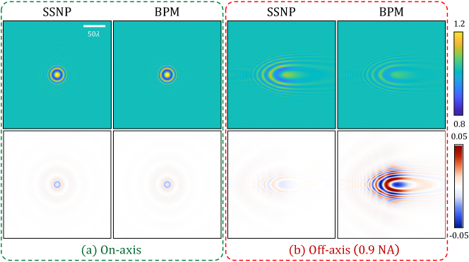
Figure 2: Simulation using the SSNP and BPM IDT models for a $6\lambda$ diameter bead ($n=1.02$) in air ($n_{0}=1$) using (a) on-axis illumination (NA = 0), and (b) off-axis illumination (NA = 0.9). The bead center is placed at the origin at $z=0$, and the observation plane is placed at $z=125\lambda$. The upper row shows the normalized intensity, and the lower row shows the difference comparing against the Mie theory.

A major benefit of the SSNP model compared with the BPM model is its higher accuracy when computing scattered field under high-NA illumination [16]. To evaluate the SSNP-IDT model’s accuracy under high-NA illumination, we simulated sequential IDT measurements of a bead using the BPM and SSNP models and compare them against the Mie scattering theory. In this simulation, the bead has an RI of 1.02 and is immersed in air ($n_{0}=1$). The diameter of the bead is $6\lambda=$3.09\text{\,}\mathrm{\SIUnitSymbolMicro m}$$ where $\lambda=$0.515\text{\,}\mathrm{\SIUnitSymbolMicro m}$$ is the wavelength. In Fig. 2, we show the on-axis and an off-axis 0.9 NA illumination case. The microscope has a 0.9 NA objective lens. The discretization steps are $(\Delta x,\Delta y,\Delta z)=(\lambda/4,\lambda/4,\lambda/8)$. The simulated intensities from the BPM and SSNP IDT models and their difference maps from the Mie theory are shown. For the on-axis illumination case, both the SSNP and BPM models agree with the Mie theory with negligible errors. For the off-axis high-NA illumination case, SSNP retains high accuracy while the BPM model suffers from more severe errors. This study confirms that our SSNP-IDT forward model is highly accurate in simulating IDT measurements under high-NA illuminations. As a result, we will use the SSNP model for simulating the measurements in the subsequent numerical studies due to its higher computational efficiency and flexibility compared to the Mie theory.

3.2 Simulation: reconstruction algorithm evaluation

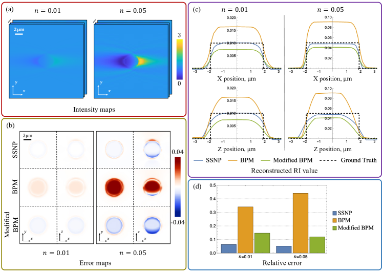
Figure 3: (a) An example image from the SSNP simulated intensity measurements for low and high RI sphere samples. (b) Error maps of the RI reconstructions from the SSNP, original BPM, and modified BPM models. The X-Y and X-Z cross sections through the center of each sphere are shown. (c) The cutlines along X and Z of the reconstructed and ground-truth RI through the center of each sphere. (d) The relative MSE of all the reconstructions.

To assess our SSNP-IDT reconstruction algorithm in the non-paraxial regime, we simulated high-NA annular IDT measurements using the SSNP-sIDT forward model and then performed reconstruction using the algorithm in Section 2.4. We simulated a $6\lambda$-diameter sphere with voxel size $(\lambda/4,\lambda/4,\lambda/8)$. To study the performance under different scattering strengths, we used two RI contrast values, including $\Delta n$=0.01 and 0.05. We simulated 8 intensity images from illuminations evenly distributed on a 0.89 NA ring, collected by a 0.9 NA objective (Fig. 3a).

We performed reconstruction using both the SSNP, the original BPM [15], and modified BPM model [16] (see details in Supplement 1) in Fig. 3b and 3c. Then we use the relative mean squared error (MSE) $\mathscr{E}$ to quantify the overall reconstruction quality in Fig. 3d, which is defined as $\mathscr{E}=\frac{{\left\lVert{n_{GT}-\hat{n}}\right\rVert}^{2}}{{\left\lVert{n_{GT}-n_{0}}\right\rVert}^{2}},$ where $n_{GT}$ and $\hat{n}$ are the ground-truth and reconstructed RI, respectively. The original BPM over-estimates the RI values in both the weakly and strongly scattering cases. This is because the BPM forward model underestimates the phase modulation for the high-NA components [16]. The modified BPM model introduces an cosine obliquity factor to compensate for the under-estimated phase modulation, which improves the model accuracy at high angles [16]. However, this approximation results in under-estimation in the reconstructed RI values. Figure 3d quantitatively shows that the SSNP model can recover the RI distribution with better accuracy compared to the BPM and modified BPM models in both the weakly and strongly scattering cases. By inspecting the cross sections and cutlines shown in Fig. 3b and 3c, we concluded that the reconstruction in all three dimensions are limited by the finite Fourier coverage provided by the illumination and imaging optics. Both the lateral resolution and the amount of axial elongation due to the “missing-cone” problem are comparable regardless of the model used.

3.3 Experiments: sequential IDT

To test our SSNP-sIDT reconstruction algorithm, we apply it to the annular IDT data from our previous publication in [7]. Briefly, our annular IDT system consists of a Nikon E200 microscope equipped with a ring LED (Adafruit, 1586 NeoPixel Ring). We used a $40\times$/$0.65$ NA (Nikon, CFI Plan Achromat) objective. The ring LED has 24 LEDs and is $60\text{\,}\mathrm{mm}$ in diameter. It is centered at the optical axis and placed approximately $35\text{\,}\mathrm{mm}$ away from the sample, which sets the illumination angle to be $\sim$$$ and matches with the objective NA. Each LED illumination is approximated as a plane wave with a wavelength $\lambda=$515\text{\,}\mathrm{nm}$$. We use the same self-calibration method as [7] to get the accurate direction of the wave vector.

In our reconstruction algorithm, the physical quantities on the XY plane, including the field, the field’s axial derivative, and the slices of the predicted RI values, are discretized on 2D grids. The grid spacing is $\Delta x=\Delta y=$0.1625\text{\,}\mathrm{\SIUnitSymbolMicro m}$$, which is chosen to be smaller than but close to $\frac{\lambda}{4\mathrm{NA}}$ to ensure both accuracy and computational efficiency of the algorithm, and is the same as the effective pixel size on the camera.

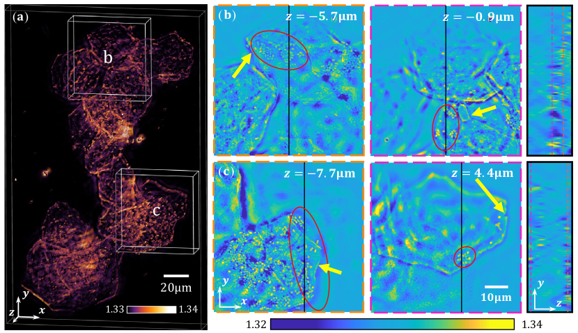
Figure 4: Reconstruction of buccal epithelial cells. (a) 3D rendering of the full-FOV reconstruction. (b), (c) Zoomed-in views of XY (Top), XZ (Bottom) cross sections. The red ellipses show the native bacteria crowded regions. The yellow arrows highlight the sharp cell boundary features.

First, we verify the reconstruction algorithm on unstained buccal epithelial cells immersed in purified water on a glass slide and covered by a coverslip. The dataset contains $24$ intensity images. The reconstructed volume is between $-9.7\text{\,}\mathrm{\SIUnitSymbolMicro m}9.7\text{\,}\mathrm{\SIUnitSymbolMicro m}$ around the focal plane, and the FOV is $162.5\text{\times}162.5\text{\,}\mathrm{\SIUnitSymbolMicro m}$. We discretized the sample volume to $150$ slices, each with $1000\times 1000$ pixels, with voxel size $0.1625\text{\times}0.1625\text{\times}0.129\text{\,}\mathrm{\SIUnitSymbolMicro m}$. To perform the reconstruction with memory-limited hardware, we cropped the full FOV into four $576\text{\times}576$-pixel subregions, reconstructed them separately, and then stitched them together. Figure 4(a) shows the 3D rendering of the reconstructed RI distribution of the entire cell cluster volume. The 3D reconstruction allows easily discriminating cells at different depths. As shown in Fig. 4(b-c), our SSNP algorithm successfully reconstructs high-resolution features, such as cell boundaries, membrane, and native bacteria around the cells.

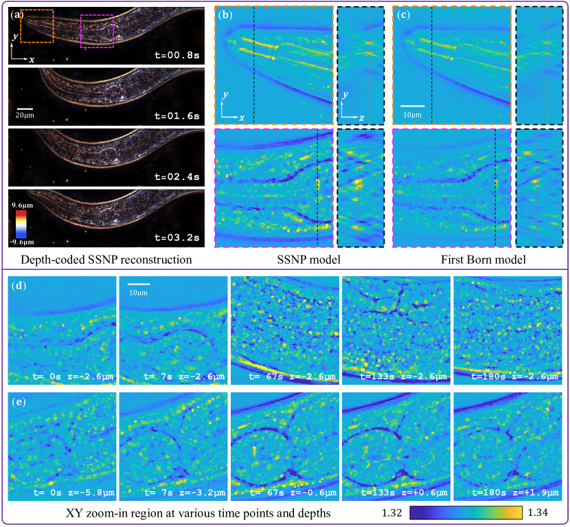
Figure 5: Reconstruction of a live C. elegans worm. (a) Color-coded depth projections of the whole worm reconstruction using SSNP model at different times. (b-c) XY and ZY cross-sections of the buccal cavity (top), part of the isthmus and terminal bulb (bottom). The reconstructions are using SSNP model and first-Born based model, respectively. (d) XY cross-sections of SSNP-IDT reconstruction at different time points of the same subregion and depth. (e) XY cross-sections of SSNP-IDT reconstruction at different depths and time points of the same subregion.

Next, we apply our algorithm to a live C. elegans worm sample. Young adult C. elegans were mounted on $3\text{\,}\mathrm{\char 37\relax}$ agarose pads in a drop of nematode growth medium (NGM) buffer. Glass coverslips were then gently placed on top of the pads and sealed with a 1:1 mixture of paraffin and petroleum jelly. The time series IDT measurements were taken at $\sim$10\text{\,}\mathrm{Hz}$$ with 8 intensity images for each set. The reconstruction is performed in a volume of $97.5\text{\times}390\text{\times}38.6\text{\,}\mathrm{\SIUnitSymbolMicro m}$ centered at the focal plane. The volume is discretized to $600\text{\times}2400\text{\times}300$ voxels with voxel size $0.1625\text{\times}0.1625\text{\times}0.129\text{\,}\mathrm{\SIUnitSymbolMicro m}$. The reconstruction is more challenging since the worm contains complex and strongly scattering features. Figure 5(a) shows four consecutive volumes reconstructed by our SSNP algorithm, displayed as color-coded depth projections. Fig. 5(b-c) shows two zoomed-in XY and YZ cross-sectional views around the buccal cavity and terminal pharyngeal bulb regions. Comparing with the SSNP model, the first-Born model underestimates the RI value and misses the low-frequency information. This effect is also reported in other multiple-scattering models for IDT reconstruction [14, 8]. Additional zoom-in regions at different depths and time points are shown in Fig. 5(d-e), containing features including the anterior bulb, vulva, lipid droplets, and body wall muscle cells inside the worm sample.

3.4 Experiment: multiplexed IDT

Next, we test our SSNP-mIDT reconstruction algorithm to process data from our previous publication in [10]. Briefly, the multiplexed IDT system consists of a Nikon TE 2000U microscope equipped with a custom LED matrix. Each LED approximately generated a plane wave with a central wavelength $\lambda=$632\text{\,}\mathrm{nm}$$. The measurements were taken with a 40$\times$ / 0.65 NA objective (Nikon, CFI Plan Achromat) and an sCMOS camera (PCO.Edge 5.5).

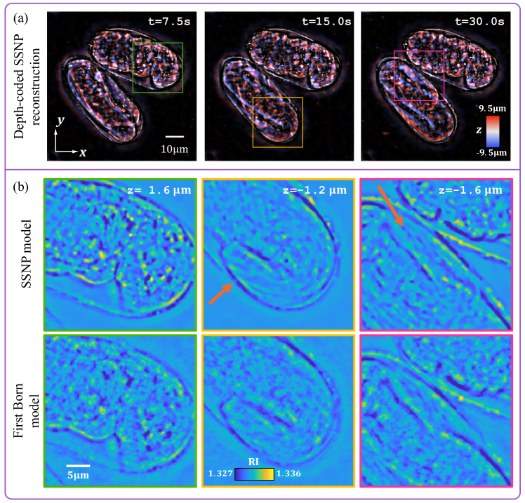
Figure 6: Reconstruction of live C. elegans embryos. (a) Color-coded depth projection of SSNP-mIDT reconstructon at $t=$7.5\text{\,}\mathrm{s}15\text{\,}\mathrm{s}30\text{\,}\mathrm{s}$$ (b-c) XY zoom-in cross sections at various times and depths using SSNP and first-Born models, which shows developing cells, buccal cavity and tail region of the embryos and worms, respectively.

We apply our algorithm to a highly scattering sample of live C. elegans embryos. The multiplexed measurement used $16$ disjoint illumination patterns, each containing 6 LEDs. In total 96 LEDs are used in this experiment, corresponding to illumination NA ranging from $0.3$ to $0.575$. We reconstructed a $81.3\text{\times}81.3\text{\times}19.0\text{\,}\mathrm{\SIUnitSymbolMicro m}$ volume, which was discretized to $500\text{\times}500\text{\times}120$ voxels with voxel size $0.1625\text{\times}0.1625\text{\times}0.158\text{\,}\mathrm{\SIUnitSymbolMicro m}$. In Fig. 6, the embryo on the left is in the late three-fold (quickening) stage, and the one on the right is in the comma stage. From the color-coded view in Fig. 6(a), how the worms are folded can be clearly observed. From the single-depth cross-sections in Fig. 6(b), the morphological details of the cells’ outline, the buccal cavity, and the tail of the worm are reconstructed. Similar to aIDT, the SSNP model reconstructs more low-frequency phase information and higher RI contrast than the first-Born model. Besides, the TV regularization used in the SSNP model effectively suppresses the noise, which helps to provide a clean background and sharp embryo boundary comparing with the Tikhonov regularization used in the first-Born model. The high acquisition rate of multiplexed IDT enabled reconstructing the developing process and the moving behavior of the embryos, as shown in the time-series reconstructions. As compared to our previous single-scattering based linear multiplexed IDT reconstruction algorithm [10], SSNP-mIDT provides more robust demultiplexing capability that removes the fuzzy diffraction artifacts inside the embryos. Since the algorithm allows independent update from individual LEDs in each pattern, it greatly suppresses the cross-talk artifacts suffered by the linear model.

4 Conclusion and discussion

In conclusion, we developed a non-paraxial multiple-scattering model for 3D RI reconstruction from both sequential and multiplexed intensity diffraction tomography measurements. The SSNP model ensures high accuracy when imaging strongly scattering samples under high-angle illumination. We demonstrated the robustness of the model on weakly scattering cells and multiple-scattering dynamic C. elegans worm and embryos. With a unified reconstruction algorithm, our model is flexible for both the sequential and multiplexed IDT setups. This treatment for multiplexed measurement can also be applied to interferometric setups and speed up the acquisition for the ODT systems [1, 16].

A major limitation of our current IDT systems is the limited angular coverage (up to 0.65 NA) that creates a significant amount of missing-cone artifacts and fundamentally limits the reconstruction quality, as shown by our numerical studies and experimental results. While several recent works alleviate the missing-cone artifacts by using higher NA (>1) optics and more than 10$\times$ more measurements [14, 8], it sacrifices the FOV and acquisition speed, which prevented them from capturing the whole worm without mechanical FOV scanning and imaging dynamic biological processes. It may be possible to integrate the annular and multiplexed illumination strategies in these systems to speed up the acquisition while achieving better Fourier coverage.

It has been shown that 3D Fourier Ptychography models based on the first-Born approximation [22] and BPM [6] can further handle dark-field measurements, which allows considering high spatial frequency information beyond the objective NA in the 3D reconstruction. Since our SSNP model can be treated as an enhancement of the first-Born and BPM models, it is possible to extend our work to incorporate additional dark-field information for high-resolution IDT reconstructions, which will be considered in our future work. Alternatively, several advanced reconstruction frameworks for IDT have been recently developed and shown promising results to greatly suppress the missing-cone artifacts, including end-to-end supervised learning [23], untrained neural network [9], model-based reconstruction with a deep denoiser [24], neural fields based reconstruction [25], and physics-informed neural network [26]. Notably, our SSNP forward model has been previously applied to generate a large-scale training data set to train a supervised learning model [23]. It is further possible to directly incorporate our SSNP model into the model-based learning strategies [9, 24, 25] in the future.

Funding National Science Foundation: 1846784.

Disclosures The authors declare no conflicts of interest.

Data availability The data and code can be found at the GitHub repository: https://github.com/bu-cisl/SSNP-IDT

Supplemental document See Supplement 1 for supporting content.

References

- [1] Y. Park, C. Depeursinge, and G. Popescu, “Quantitative phase imaging in biomedicine,” \JournalTitleNature Photonics 12, 578–589 (2018).
- [2] D. Jin, R. Zhou, Z. Yaqoob, and P. T. C. So, “Tomographic phase microscopy: principles and applications in bioimaging [invited],” \JournalTitleJ. Opt. Soc. Am. B 34, B64–B77 (2017).
- [3] T. Kim, R. Zhou, M. Mir, S. D. Babacan, P. S. Carney, L. L. Goddard, and G. Popescu, “White-light diffraction tomography of unlabelled live cells,” \JournalTitleNature Photonics 8, 256–263 (2014).
- [4] G. Gbur and E. Wolf, “Diffraction tomography without phase information,” \JournalTitleOpt. Lett. 27, 1890–1892 (2002).
- [5] R. Ling, W. Tahir, H.-Y. Lin, H. Lee, and L. Tian, “High-throughput intensity diffraction tomography with a computational microscope,” \JournalTitleBiomed. Opt. Express 9, 2130–2141 (2018).
- [6] L. Tian and L. Waller, “3D intensity and phase imaging from light field measurements in an LED array microscope,” \JournalTitleOptica 2, 104 (2015).
- [7] J. Li, A. Matlock, Y. Li, Q. Chen, C. Zuo, and L. Tian, “High-speed in vitro intensity diffraction tomography,” \JournalTitleAdvanced Photonics 1, 1–13 (2019).
- [8] M. Chen, D. Ren, H.-Y. Liu, S. Chowdhury, and L. Waller, “Multi-layer born multiple-scattering model for 3d phase microscopy,” \JournalTitleOptica 7, 394–403 (2020).
- [9] K. C. Zhou and R. Horstmeyer, “Diffraction tomography with a deep image prior,” \JournalTitleOpt. Express 28, 12872–12896 (2020).
- [10] A. Matlock and L. Tian, “High-throughput, volumetric quantitative phase imaging with multiplexed intensity diffraction tomography,” \JournalTitleBiomedical Optics Express 10, 6432 (2019).
- [11] J. Li, N. Zhou, J. Sun, S. Zhou, Z. Bai, L. Lu, Q. Chen, and C. Zuo, “Transport of intensity diffraction tomography with non-interferometric synthetic aperture for three-dimensional label-free microscopy,” \JournalTitleLight: Science & Applications 11 (2022).
- [12] A. B. Ayoub, A. Roy, and D. Psaltis, “Optical diffraction tomography using nearly in-line holography with a broadband led source,” \JournalTitleApplied Sciences 12 (2022).
- [13] R. Horstmeyer, J. Chung, X. Ou, G. Zheng, and C. Yang, “Diffraction tomography with fourier ptychography,” \JournalTitleOptica 3, 827–835 (2016).
- [14] S. Chowdhury, M. Chen, R. Eckert, D. Ren, F. Wu, N. Repina, and L. Waller, “High-resolution 3D refractive index microscopy of multiple-scattering samples from intensity images,” \JournalTitleOptica 6, 1211 (2019).
- [15] U. S. Kamilov, I. N. Papadopoulos, M. H. Shoreh, A. Goy, C. Vonesch, M. Unser, and D. Psaltis, “Optical Tomographic Image Reconstruction Based on Beam Propagation and Sparse Regularization,” \JournalTitleIEEE Transactions on Computational Imaging 2, 59–70 (2016).
- [16] J. Lim, A. B. Ayoub, E. E. Antoine, and D. Psaltis, “High-fidelity optical diffraction tomography of multiple scattering samples,” \JournalTitleLight: Science & Applications 8, 82 (2019).
- [17] A. Sharma and A. Agrawal, “New method for nonparaxial beam propagation,” \JournalTitleJ. Opt. Soc. Am. A 21, 1082–1087 (2004).
- [18] L.-H. Yeh, J. Dong, J. Zhong, L. Tian, M. Chen, G. Tang, M. Soltanolkotabi, and L. Waller, “Experimental robustness of fourier ptychography phase retrieval algorithms,” \JournalTitleOpt. Express 23, 33214–33240 (2015).
- [19] Z. Wu, Y. Sun, A. Matlock, J. Liu, L. Tian, and U. S. Kamilov, “SIMBA: Scalable Inversion in Optical Tomography Using Deep Denoising Priors,” \JournalTitleIEEE Journal on Selected Topics in Signal Processing 14, 1163–1175 (2020).
- [20] W. Wirtinger, “Zur formalen Theorie der Funktionen von mehr komplexen Veränderlichen,” \JournalTitleMathematische Annalen 97, 357–375 (1927).
- [21] L. Tian, X. Li, K. Ramchandran, and L. Waller, “Multiplexed coded illumination for fourier ptychography with an led array microscope,” \JournalTitleBiomed. Opt. Express 5, 2376–2389 (2014).
- [22] C. Zuo, J. Sun, J. Li, A. Asundi, and Q. Chen, “Wide-field high-resolution 3d microscopy with fourier ptychographic diffraction tomography,” \JournalTitleOptics and Lasers in Engineering 128, 106003 (2020).
- [23] A. Matlock and L. Tian, “Physical model simulator-trained neural network for computational 3d phase imaging of multiple-scattering samples,” \JournalTitlearXiv:2103.15795 (2021).
- [24] Z. Wu, Y. Sun, A. Matlock, J. Liu, L. Tian, and U. S. Kamilov, “Simba: Scalable inversion in optical tomography using deep denoising priors,” \JournalTitleIEEE Journal of Selected Topics in Signal Processing 14, 1163–1175 (2020).
- [25] R. Liu, Y. Sun, J. Zhu, L. Tian, and U. Kamilov, “Zero-shot learning of continuous 3d refractive index maps from discrete intensity-only measurements,” \JournalTitlearXiv:2112.00002 (2021).
- [26] A. B. Ayoub, A. Saba, C. Gigli, and D. Psaltis, “Optical diffraction tomography based on 3d physics-inspired neural network (PINN),” \JournalTitlearXiv:2206.05236 (2022).