Reachability Analysis of a General Class of Neural Ordinary Differential Equations

Abstract

Continuous deep learning models, referred to as Neural Ordinary Differential Equations (Neural ODEs), have received considerable attention over the last several years. Despite their burgeoning impact, there is a lack of formal analysis techniques for these systems. In this paper, we consider a general class of neural ODEs with varying architectures and layers, and introduce a novel reachability framework that allows for the formal analysis of their behavior. The methods developed for the reachability analysis of neural ODEs are implemented in a new tool called NNVODE. Specifically, our work extends an existing neural network verification tool to support neural ODEs. We demonstrate the capabilities and efficacy of our methods through the analysis of a set of benchmarks that include neural ODEs used for classification, and in control and dynamical systems, including an evaluation of the efficacy and capabilities of our approach with respect to existing software tools within the continuous-time systems reachability literature, when it is possible to do so.

1 Introduction

Neural Ordinary Differential Equations (ODEs) were first introduced in 2018, as a radical new neural network design that boasted better memory efficiency, and an ability to deal with irregularly sampled data [21]. The idea behind this family of deep learning models is that instead of specifying a discrete sequence of hidden layers, we instead parameterize the derivative of the hidden states using a neural network [8]. The output of the network can then be computed using a differential equation solver [8]. This work has spurred a whole range of follow-up work, and since 2018 several variants have been proposed, such as augmented neural ODEs (ANODEs) and their ensuing variants [39, 11, 16]. These variants provide a more expressive formalism by augmenting the state space of neural ODEs to allow for the flow of state trajectories to cross. This crossing, prohibited in the original framework, allows for the learning of more complex functions that were prohibited by the original neural ODE formulation [11].

Due to the potential that neural networks boast in revolutionizing the development of intelligent systems in numerous domains, the last several years have witnessed a significant amount of work towards the formal analysis of these models. The first set of approaches that were developed considered the formal verification of neural networks (NN), using a variety of techniques including reachability methods [46, 47, 3, 40], and SAT techniques [29, 30, 13]. Thereafter, many researchers proposed novel formal method approaches for neural network control systems (NNCS), where the majority of methods utilized a combination of NN and hybrid system verification techniques [14, 22, 44, 26, 23, 6]. Building on this work, a natural outgrowth is extending these approaches to analyze and verify neural ODEs, and some recent studies have considered the analysis of formal properties of neural ODEs. One such study aims to improve the understanding of the inner operation of these networks by analyzing and experimenting with multiple neural ODE architectures on different benchmarks [36]. Some studies have considered analyses of the robustness of neural ODEs such as [7] and [48], which evaluate the robustness of image classification neural ODEs and compare the efficacy of this class of network against other more traditional image classifier architectures. The first reachability technique targeted for neural ODEs presented a theoretical regime for verifying neural ODEs using Stochastic Lagrangian Reachability (SLR) [19]. This method is an abstraction-based technique that computes confidence intervals for the calculated reachable set with probabilistic guarantees. In a follow-up work, these methods were improved and implemented in a tool called Gotube [20], which is able to compute reach sets for longer time horizons than most state-of-the-art reachability tools. However, these methods only provide stochastic bounds on the reach sets, so there are no formal guarantees on the derived results.

To the best of our knowledge, this paper presents the first deterministic verification framework for a general class of neural ODEs with multiple continuous-time and discrete-time layers. In this work, we present our verification framework NNVODE that makes use of deterministic reachability approaches for the analysis of neural ODEs. Our methods are evaluated on a set of benchmarks with different architectures and conditions in the area of dynamical systems, control systems, and image classification. We also compare our results against three state-of-the-art verification tools when possible. In summary, the contributions of this paper are:

• We introduce a general class of neural ODEs that allows for the combination of multiple continuous-time and discrete-time layers.

• We develop NNVODE, an extension of NNV [46], to formally analyze a general class of neural ODEs using sound and deterministic reachable methods.

• We run an extensive evaluation on a collection of benchmarks within the context of time-series analysis, control systems, and image classification. We compare the results to Flow*, GoTube, and JuliaReach for neural ODE architectures where this is possible.

2 Background and Problem Formulation

Neural ODEs emerged as a continuous-depth variant of neural networks becoming a special case of ordinary differential equations (ODEs), where the derivatives are defined by a neural network, and can be expressed as:

$$\dot{z}=g(z),\quad\quad\quad z(t_{0})=z_{0},$$ (1)

where the dynamics of the function $g:\mathbb{R}^{j}\rightarrow{}\mathbb{R}^{p}$ are represented as a neural network, and initial state $z_{0}\in\mathbb{R}^{j}$, where $j$ corresponds to the dimensionality of the states $z$. A neural network (NN) is defined to be a collection of consecutively connected $\mathscr{NN}$-Layers as described in Definition 1.

Definition 1 ($\mathscr{NN}$-Layer)

A $\mathscr{NN}$-Layer is a function h: $\mathbb{R}^{j}\rightarrow{}\mathbb{R}^{p}$, with input x $\in$ $\mathbb{R}^{j}$, output y $\in$ $\mathbb{R}^{p}$ defined as follows

$$y=h(x)$$ (2)

where the function $h$ is determined by parameters $\theta$, typically defined as a tuple $\theta$ = $\langle$$\sigma$,W,b$\rangle$ for fully-connected layers, where W $\in$ $\mathbb{R}^{j\times p}$, b $\in$ $\mathbb{R}^{p}$, and activation function $\sigma$: $\mathbb{R}^{j}\rightarrow{}\mathbb{R}^{p}$, thus the fully-connected $\mathscr{NN}$-Layer is described as

$$y=h(x)=\sigma(\textbf{W}(x)+\textbf{b}).$$ (3)

However, for other layers such as convolutional-type $\mathscr{NN}$-Layers, $\theta$ may include parameters like the filter size, padding, or dilation factor and the function $h$ in  (3) may not necessarily apply. For a formal definition and description of the reachability analysis for each of these layers that are integrated within NNVODE, we refer the reader to Section 4 of [43]. For the Neural ODEs (NODEs), we assume that $g$ is Lipschitz continuous, which guarantees that the solution of $\dot{z}=g(z)$ exists. This assumption allows us to model $g$ with $m$ layers of continuously differentiable activation functions $\sigma_{k}$ for $k\in\{1,2,...,m\}$ such as sigmoid, tanh, and exponential activation functions. Described in  (1) is the notion of a NODE as introduced in [8] and an example is illustrated in Figure 1.

Definition 2 (NODE)

A NODE is a function $\dot{z}=g(z)$ with $m$ fully-connected $\mathscr{NN}$-Layers, and it is defined as follows

$$\dot{z}=g(z)=h_{m}(h_{m-1}(...h_{1}(z))),$$ (4)

where $g:\mathbb{R}^{j}\rightarrow{}\mathbb{R}^{p}$, $\sigma_{k}:\mathbb{R}^{j_{k}}\rightarrow{}\mathbb{R}^{p_{k}}$, $\textbf{W}_{k}\in\mathbb{R}^{j_{k}\times p_{k}}$, and $\textbf{b}_{k}\in\mathbb{R}^{p_{k}}$. For each layer $k$=$\{1,2,\dots,m\}$, we describe the function $h_{k}$ as in  (3).

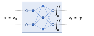
Figure 1: Illustration of an example of NODE, as defined in (1) and  (4), and Definition 2.

An example of NODE with m = 2 hidden layers, 2 inputs and 2 outputs is depicted in Figure 1.

2.1 General Neural ODE

The general class of neural ODEs (GNODEs) considered in this work is more complex than previously analyzed neural ODEs as it may be comprised of two types of layer: NODEs and $\mathscr{NN}$-Layers. We introduce a more general framework where multiple NODEs can make up part of the overall architecture along with other $\mathscr{NN}$-Layers, as described in Definition 3. This is the reachability problem subject of evaluation in this work.

Definition 3 (GNODE)

A GNODE $~{}\mathcal{F}$ is any sequence of consecutively connected $N$ layers $\mathcal{L}_{k}$ for $k\in\{1,\dots N\}$ with $N_{O}$ NODEs and $N_{D}$ $\mathscr{NN}$-Layers, that meets the conditions $1\leq N_{O}\leq N$, $0\leq N_{D}<N$, and $N_{D}$ + $N_{O}$ = $N$.

With the above definition, we formulate a theorem for the restricted class of neural ODEs (NODE) that we use to compare our methods against existing techniques.

Observation 1 (Special case 1: NODE)

Let $\mathcal{F}$ be a GNODE with $N$ layers. If $N=1$, $N_{O}=1$ and $N_{D}=0$, then $\mathcal{F}$ is equivalent to an ODE whose continuous-time dynamics are defined as a neural network, and we refer to it as a NODE (as in Definition 2).

In Figure 2, an example of a GNODE is shown, which has 1 input (x), 1 output (y), $N_{O}$ = 2 NODEs, and $N_{D}$ = 5 $\mathscr{NN}$-Layers, with its 5 numbered segments described as: 1) The first segment has a $\mathscr{NN}$-Layer, with one hidden layer of 2 neurons and an output layer of 2 neurons, 2) a NODE with one hidden layer of 3 neurons and an output layer of 2 neurons, 3) $\mathscr{NN}$-Layer with 3 hidden layers of 4,1, and 2 neurons respectively, and an output layer of 2 neurons, 4) NODE with a hidden layer of 3 neurons and output layer of 2 neurons, and 5) $\mathscr{NN}$-Layer with a hidden layer of 4 neurons and and output layer with 1 neurons.

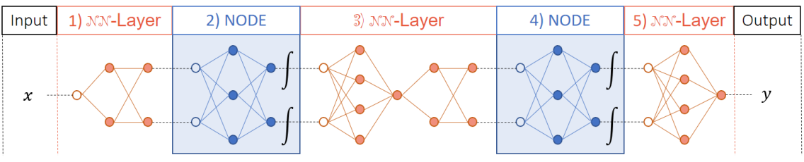
Figure 2: Example of a GNODE. The filled circles represent weighted neurons in each layer, non-filled neurons represent the inputs of each layer-type segment, shown for visualization purposes.

Given this GNODE architecture, we are capable of encoding the originally proposed neural ODE [8], as well as several of its model improvements including higher-order neural ODEs like the second-order neural ODE (SONODE) [39], augmented neural ODEs (ANODEs) [11], and input-layer augmented neural ODEs (ILNODEs). This general class of neural ODEs from Definition 3 is applicable to many applications including image classification, time series prediction, dynamical system modeling and normalizing flows.

Observation 2 (Special case 2 - NNCS)

We can consider the NNCS as a special case of the GNODE, as the NNCS models also consist of $\mathscr{NN}$-Layers and NODE, under the assumption that the plant is described as an NODE. NNCS in the general architecture have $\mathscr{NN}$-Layers followed by an ODE or NODE, which connects back to the $\mathscr{NN}$-Layers in a feedback loop manner for $cp$ control steps. Thus, by unrolling the NNCS $cp$ times, we consecutively connect the $\mathscr{NN}$-Layers with the NODE, creating a GNODE.

2.2 NODE: Applications

There are two application modes of a NODE, model reduction and dynamical systems. On one hand, we can use it as a substitute for multiple similar layers to reduce the depth and overall size of a model [8]. In this context, we treat the NODE as an input-output mapping function, and set the integration time $t_{f}$ to a fixed number during training, which will be then used during simulation or reachability. Typically, this value is set to 1. On the other hand, we can make use of NODEs to capture the behavior of time-series data or dynamical systems. In this sense, $t_{f}$ is not fixed, and it will be determined by the user/application. In summary, we can use NODEs for: 1) time-series or dynamical system modeling, and 2) model reduction. For time-series, $t_{f}$ is variable, user or application dependent. For model reduction, $t_{f}$ is a parameter of the model fixed before training. Only the output value at time = $t_{f}$ is used, while for the time-series models, we are interested in the interval [0,$t_{f}$].

2.3 Reachability Analysis

The main focus of this manuscript is to introduce a framework for the reachability analysis of GNODEs. This framework combines set representations and methods from Neural Network (NN), Convolutional Neural Network (CNN) and hybrid systems reachability analysis. Similar to neural network reachability in NNV [46], we consider the set propagation through each layer as well as the set conversion between layers for all reachability methods for the supported layers. Hence, the reachability problem of GNODE is defined as follows:

Definition 4 (Reachable Set of a GNODE)

Let $\mathcal{F}$: $\mathbb{R}^{j}\rightarrow{}\mathbb{R}^{p}$ be a GNODE with $N$ layers. The output reachable set $\mathcal{R}_{N}$ of a GNODE with input set $\mathcal{R}_{0}$ is defined as:

$$\begin{split}\mathcal{R}_{1}&\triangleq\{y_{1}~{}|~{}y_{1}=f_{1}(y_{0}),~{}y_{0}\in\mathcal{R}_{0}\},\\ \mathcal{R}_{2}&\triangleq\{y_{2}~{}|~{}y_{2}=f_{2}(y_{1}),~{}y_{1}\in\mathcal{R}_{1}\},\\ &\vdots\\ \mathcal{R}_{N}&\triangleq\{y_{N}~{}|~{}y_{N}=f_{N}(y_{N-1}),~{}y_{N-1}\in\mathcal{R}_{N-1}\},\\ \end{split}$$ (5)

where $f_{i}$: $\mathbb{R}^{j_{i}}\rightarrow{}\mathbb{R}^{p_{i}}$ is the function $f$ of layer $i$, where $f$ is either a NODE (g) or a $\mathscr{NN}$-Layer (h).

The proposed solution to this problem is sound and incomplete, in other words, an over-approximation of the reachable set. This means that, given a set of inputs, we compute an output set of which, given any point in the input set, we simulate the GNODE and the output point is always contained within the reachable output set (sound). However, it is incomplete because the opposite is not true; there may be points in the output reachable set that cannot be traced back to be within the bounds of the input set.

Definition 5 (Soundness)

Let $\mathcal{F}$: $\mathbb{R}^{j}$ $\rightarrow{\mathbb{R}^{p}}$ be a GNODE with an input set $\mathcal{R}_{0}$ and output reachable set $\mathcal{R}_{f}$. The computed $\mathcal{R}_{f}$ given $\mathcal{F}$ and $\mathcal{R}_{0}$ is sound iff $\forall$$x$ $\in$ $\mathcal{R}_{0}$, $|$ $y$ = $\mathcal{F}$($x$), $y$ $\in$ $\mathcal{R}_{f}$.

Definition 6 (Completeness)

Let $\mathcal{F}$: $\mathbb{R}^{j}$ $\rightarrow{\mathbb{R}^{p}}$ be a GNODE with an input set $\mathcal{R}_{0}$ and output reachable set $\mathcal{R}_{f}$. The computed $\mathcal{R}_{f}$ given $\mathcal{F}$ and $\mathcal{R}_{0}$ is complete iff $\forall$$x$ $\in$ $\mathcal{R}_{0}$, $\exists$$y$ = $\mathcal{F}$($x$) $|$ $y$ $\in$ $\mathcal{R}_{f}$ and $\forall$$y$ $\in$ $\mathcal{R}_{f}$, $\exists$$x$ $\in$ $\mathcal{R}_{0}$ $|$ $y$ = $\mathcal{F}$($x$).

Definition 7 (Reachable set of a $\mathscr{NN}$-Layer)

Let h: $\mathbb{R}^{j}\rightarrow{}\mathbb{R}^{p}$ be a $\mathscr{NN}-Layer$ as described in Definition 1. The reachable set $\mathcal{R}_{h}$, with input $\mathcal{X}\subset\mathbb{R}^{n}$ is defined as

$$\centering\mathcal{R}_{h}=\{y~{}|~{}y=h(x),x\in\mathcal{X}\}.\@add@centering$$

Definition 7 applies to any discrete-time layer that is part of a GNODE, including, but not limited to the following supported $\mathscr{NN}-Layers$ supported in NNVODE: fully-connected layers with ReLU, tanh, sigmoid and leaky-ReLU activation functions, and convolutional-type layers such as batch normalization, 2-D convolutional, and max-pooling.

The reachability analysis of NODEs is akin to the general reachability problem for any continuous-time system modeled by an ODE. If we represent the NODE as a single layer $i$ of a GNODE with continuous dynamics described by  (1), and assume that for a given initial state $z_{0}\in\mathbb{R}^{j_{i}}$, the system admits a unique trajectory defined on $\mathbb{R}^{+}_{0}$, described by $\zeta(.,z(t_{0}))$, then the reachable set of the given NODE can be characterized by Definition 8.

Definition 8 (Reachable set of a NODE)

Let $g$ be a NODE with solution $\zeta$(t; z₀) to  (1) for initial state z₀. The reachable set, $\mathcal{R}_{g}$ at $t=t_{F}$, $\mathcal{R}_{g}(t_{F})$, with initial set $\mathcal{R}_{0}\subset\mathbb{R}^{n}$ at time $t=t_{0}$ is defined as

$$\centering\mathcal{R}_{g}(t_{F})=\{\zeta(t;z_{0})\in\mathbb{R}^{n}~{}|~{}z_{0}\in\mathcal{R}_{0},t\in[0,t_{f}]\}.\@add@centering$$

We also describe the reachable set for a time interval [$t_{0}$,$t_{f}$] as follows

$$\mathcal{R}_{g}([t_{0},t_{f}]):=\bigcup_{t\in[t_{0},t_{f}]}\mathcal{R}_{g}(t)$$

Now that we have outlined the general reachability problem of a NODE, whether we compute a single reachable set for the NODE at $t$ = $t_{F}$, or over an interval $t$ $\in$ [$t_{0}$,$t_{F}$] (computed by get$\_$time()), depends on how the neural ODE was trained and the specific application of its use. However, the core computation remains the same. This is outlined in Algorithm 1.

Algorithm 1 Reachability analysis of a GNODE.

1:$\mathcal{F},\mathcal{R}_{0}$   $//$ GNODE, input set

2:$\mathcal{R}_{f}$  $//$ output reachable set

3:procedure $\mathcal{R}_{f}$ = reach($\mathcal{F},\mathcal{R}_{0}$)

4:    N = $\mathcal{F}$.layers   $//$ number of layers

5:    for i = 1 : N do   $//$ loop through every layer

6:         $\mathscr{L}_{i}$ = $\mathcal{F}$.layer(i)

7:         if $\mathscr{L}_{i}$ $is$ NODE  then  $//$ check layer type

8:             $\textbf{t}_{i}$ = get$\_$time($\mathscr{L}_{i}$)   $//$ get integration time bounds of layer $i$

9:             $\mathcal{R}_{i}$ = reach_NODE($\mathscr{L}_{i}$,$\mathcal{R}_{i-1}$, $\textbf{t}_{i}$)   $//$ reach set of layer $i$, Definition 8

10:         else

11:             $\mathcal{R}_{i}$ = reach_NN($\mathscr{L}_{i}$, $\mathcal{R}_{i-1}$)   $//$ reach set of layer $i$, Definition 7              

12:    $\mathcal{R}_{f}$ = $\mathcal{R}_{N}$   $//$ output reachable set

2.4 Reachability Methods

In the previous sections, we defined the reachable set of a GNODE using a layer-by-layer approach. However, the computation of these reachable sets is defined by the reachability methods and set representations utilized in their construction. For instance, the same operations are not utilized to compute the reachable set for a fully-connected layer with a hyperbolic tangent activation function as with a fully convolutional layer. In the following section, we describe the set of methods in the NNVODE tool available to the community to compute the reachable set of each specific layer.

We begin with the NODE approaches, where we make a distinction based on the underlying dynamics. If the NODE is nonlinear, we make use of zonotope and polynomial-zonotope based methods that are implemented and available in CORA [1, 2]. If the NODE is purely linear, then we utilize the star set-based methods introduced in [5], which are more scalable than other zonotope-based methods and possess soundness guarantees as well.

For the $\mathscr{NN}$-Layers, there are several methods available, including zonotope-based and star-set based methods. However, we limited our implementation only using star sets to handle these layers, as this representation was demonstrated to be more computationally efficient and to enable tighter over-approximations of the derived reachable sets than zonotope methods [45]. Additionally, in using star set methods, we allow for the use of both approximate methods (approx-star) and exact methods (exact-star). A summary of these methods and supported layers is depicted in Table 1, and for a complete description of the reachability methods utilized in our work, we refer the reader to [46] and the manual.

Table 1: Layers supported in NNVODE and reachability sets and methods available.

Layer Type – Set Rep. (method name) NODE Linear – Star-set ("direct") [5] NODE Nonlinear – Zonotope, Polynomial Zonotope * [1, 2] $\mathscr{NN}$-Layer FC: linear, ReLU – Star-set ("approx-star", "exact-star") [45] $\mathscr{NN}$-Layer FC: leakyReLU, tanh, sigmoid, satlin – Star-set ("approx-star") [46] $\mathscr{NN}$-Layer Conv2D – ImageStar ("approx-star", "exact-star") [46] $\mathscr{NN}$-Layer BatchNorm – ImageStar ("approx-star", "exact-star") [46] $\mathscr{NN}$-Layer MaxPooling2D – ImageStar ("approx-star", "exact-star") [46] $\mathscr{NN}$-Layer AvgPooling2D – ImageStar ("approx-star", "exact-star") [46] * We support several methods available using Zonotope and PolyZonotopes, which includes user-defined fixed reachability parameters ("ZonoF", "PolyF") as well as adaptive reachability methods ("ZonoA" and "PolyA"), which require no prior knowledge on reach methods or systems to verify to produce relevant results.

Implementation. One of the key aspects of the verification of GNODEs is the proper encoding of the NODEs within reachability schemes. Depending on the software that is used, this process may vary and require distinct steps. As an example, some tools, like NNVODE, are simpler and allow for matrix multiplications within the definition of equations. However, for tools like Flow*, the set of steps required to properly encode this problem are more complex as it requires a definition for each individual equation of the state derivative. Thus, a more general conversion is needed, which is illustrated in the Appendix.

3 Evaluation

Having described the details of our reachability definitions, algorithm, and implementation, we now present the experimental evaluation of our proposed work. We begin by presenting, a method and tool comparison analysis against GoTube [20], Flow* [9] and JuliaReach [6]. Then, we present a case study of an Adaptive Cruise Control system, and conclude with an evaluation of the scalability of our techniques using a random set of architectures for dynamical system applications as well as a set of classification models for MNIST. The GNODE architectures for each benchmark can be found in the Appendix. To facilitate the reproducibility of our experiments, we set a timeout of 2 hours (7200 seconds) for each reach set computation. All our experiments were conducted on a desktop with the following configuration: Intel Core i7-7700 CPU @ 3.6GHz 8 core Processor, 64 GB Memory, and 64-bit Ubuntu 16.04.3 LTS OS.

3.1 Method and Tool Comparison

We have implemented several methods within NNVODE, and the first evaluation consists of comparing the available methods for nonlinear NODEs, fixed-step zonotope and polynomial zonotopes (zono-F,poly-F) and adaptive zonotope and polynomial zonotope (zono-A,poly-A) based methods [1]. For all other $\mathscr{NN}$-Layers in the GNODEs, we use the star-set over-approximate methods. We considered multiple models, all inspired by the ILNODE representation that was introduced by Massaroli. They consist of a set of models with a varying number of augmented dimensions. All these models are instances of the GNODE class presented in Definition 3, which present an architecture of the form $\mathscr{NN}$-Layers + NODE + $\mathscr{NN}$-Layers. In this context, we were concerned with how the methods scale with respect to the number of dimensions of each model.

Table 2: Computation time of the reachability analysis of the Damped Oscillator benchmark. Results are shown in seconds with up to one decimal place.

Aug. Dims Zono-F Zono-A Poly-F Poly-A 0 34.0 574.5 201.7 654.0 1 146.4 4205.0 1573.9 3440.9 2 441.0 – – –

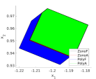
(a) Aug. Dims = 0

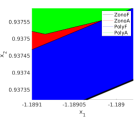
(b) Aug. Dims = 0

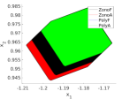
(c) Aug. Dims = 1

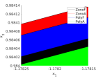
(d) Aug. Dims = 1

Figure 3: Reach sets comparison of the Damped Oscillator benchmark of the model with 0 and 1 augmented dimensions. Plots (a) and (c) show the reachable set at $t$ = 1s, and plots b) and d) show the zoomed-in reach sets to observe the minor size differences between the four methods: ZonoA, ZonoF, PolyF and PolyA.

In Table 2, we observe that the Zono-$F$ method is the fastest across all models, while the adaptive methods are the slowest. Moreover, only Zono-$F$ is able to complete the reach set computation for all three models, while the other methods time out. In terms of the size of the computed reach sets, we compare the last reach set obtained in Figure 3. In the subplots 3(b) and 3(d) we see the zoomed in reach sets, and observe that the Poly-$A$ method computes the smallest over-approximate reach set across both experiments. Based on these results, in all subsequent experiments, we use the zono-F method for nonlinear NODEs, the direct method for linear NODEs, and the over-approximate star-set methods for all the $\mathscr{NN}$-Layers.

The next part of our evaluation consists of comparing NNVODE’s methods for NODEs to those of Flow* [9], Gotube [20] and JuliaReach [6] across a collection of benchmarks that include a linear and nonlinear 2-dimensional spiral [8], a Fixed-Point Attractor (FPA) [38] and a controlled cartpole [18]. The computationn reachability results are displayed in Table 3 with the intention to characterize major differences between tools, i.e., to show some tools are 10$\times$ to 20$\times$ faster than others for some benchmarks. It is worth noting, that we are not experts on every tool that we considered. Thus it may be possible to optimize the reachable set computation for each benchmark with depending on the tool. However, we did not do so. Instead, we attempted around 3 to 5 different parameter combinations for each benchmark, and used the best results we could obtain when comparing against the other tools. The details can be found in the Appendix. The first three rows correspond to the linear spiral 2D model, and the subsequent three rows to the nonlinear one. The first set of observations that can be made in this context is that Flow* times out on all problems involving nonlinear neural ODEs, and that GoTube cannot obtain a solution to the reachability problem for the linear model. In terms of computation time, the results vary. Flow* is the fastest for the linear Spiral 2D model, regardless of the size of the initial set. In general, JuliaReach and NNVODE are much faster than GoTube, with JuliaReach being the fastest tool across the board. Additionally, there is not a significant difference between NNVODE and JuliaReach in the treatment of the nonlinear spiral model and FPA models. However, JuliaReach is an order of magnitude faster than NNVODE and two orders of magnitude faster than GoTube on the cartpole benchmark. In Figure 4 we display a subset of the reachability results from Table 3 where we observe that JuliaReach is able to compute smaller over-approximations of the reachable set on all the benchmarks except for the linear spiral model. Notably, in most cases, GoTube computes the largest over-approximation, and this effect grows far more significantly than the other tools when the complexity of the model increases. This can be observed in Figures 4(d) and 4(h).

Table 3: Results of the reachability analysis of the NODE benchmarks. All results are shown in seconds. TH stands for Time Horizon and $\delta_{\mu}$ to the input uncertainty.

Name TH ($s$) $\delta_{\mu}$ Flow* GoTube JuliaReach NNVODE (ours) Spiral${}_{L_{1}}$ 10 0.01 4.0 – 10.2 8.0 Spiral${}_{L_{2}}$ 10 0.05 3.7 – 7.2 7.4 Spiral${}_{L_{3}}$ 10 0.1 3.7 – 7.2 7.3 Spiral${}_{NL_{1}}$ 10 0.01 – 106.4 58.9 47.4 Spiral${}_{NL_{2}}$ 10 0.05 – 106.7 41.7 46.2 Spiral${}_{NL_{3}}$ 10 0.1 – 106.5 41.9 46.2 FPA₁ 0.5 0.01 - 13.6 1.9 1.3 FPA₂ 2.5 0.01 - 42.4 5.6 6.6 FPA₃ 10.0 0.01 - 140.2 28.4 7.5 Cartpole₁ 0.1 1$e$-4 - 183.0 3.2 67.9 Cartpole₂ 1.0 1$e$-4 - 1590.9 13.8 404.3 Cartpole₃ 2.0 1$e$-4 - 3065.7 35.5 834.7

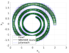
(a) Spiral${}_{L_{3}}$

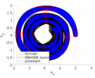
(b) Spiral${}_{NL_{3}}$

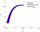
(c) FPA₃

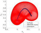
(d) Cartpole₃

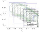
(e) Spiral${}_{L_{3}}$

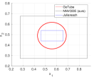
(f) Spiral${}_{NL_{3}}$

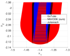
(g) FPA₃

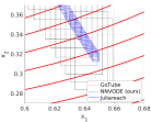
(h) Cartpole₃

Figure 4: NODE reach set comparisons. The top 4 figures ([$a$,$d$]) show the complete reachable sets of each benchmark, while the bottom 4 correspond to the zoomed-in reach sets ($e$, $g$) and to the zoomed-in figure of the last reach set ($f$,$h$). The figures show the computed reach sets of GoTube, NNVODE, JuliaReach and Flow*.

3.2 Case Study: Adaptive Cruise Control (ACC)

This case study was selected to evaluate an original NNCS benchmark used in all the AINNCS ARCH-Competitions [27, 28, 34, 46] against NNCS with NODEs as dynamical plants learned from simulation data using 3^rd order NODEs [39]. We demonstrate the verification of the ACC with different GNODEs learned as the plant model of the ACC and compare against the original benchmark, while using the same NN controller across all three models. The details of the original ACC NNCS benchmark can be found in [46], and the architectures of the third order neural ODEs can be found in the Appendix.

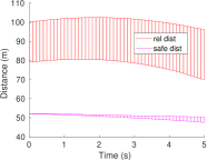
(a) Original

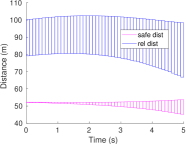
(b) Linear NODE

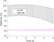
(c) Nonlinear NODE

Figure 5: Adaptive Cruise Control comparison. In red we display the relative distance of the original plant, in blue the linear NODE, in black the nonlinear NODE, and in magenta, the safe distance.

We considered all three models using the same initial conditions and present the results in Figure 5. The reachable sets obtained from all three plants are largely similar, and we can guarantee that all the models are safe since the intersection between the safe distance and the relative distance is empty. When we consider the size of the reachable sets, one can see that the original model returns the smallest reach set, whereas the linear model boasts the largest one. In all, the biggest difference between the plant dynamics is the computation time. Here, the linear 3^rd order NODE boasts the fastest computation time of 0.86 seconds, whereas the original plant takes 14.9 seconds, and the nonlinear 3^rd order NODE takes 998.7 seconds.

3.3 Classification NODEs

Our second set of experiments considered performing a robustness analysis for a set of MNIST classification models with only fully-connected $\mathscr{NN}$-Layers and other 3 models with convolutional layers as well. There is one linear NODE in each model, and we vary the number of parameters and states across all of them to study the scalability of our methods. We evaluate the robustness of these models under an L_∞ adversarial perturbation of $\epsilon$ = $\{$0.05, 1, 2$\}$ over all the pixels, and $\epsilon$ = $\{$2.55, 12.75, 25.5$\}$ over a subset of pixels (80). The complete evaluation of this benchmark consists of a robustness analysis using 50 randomly sampled images for each attack. We compare the number of images the neural ODEs are robust to, as well as the total computation time to run the reachability analysis for each model in Table 4.

Definition 9 (Robustness)

Given a classification-based GNODE $\mathcal{F}(z)$, input $z\in\mathbb{R}^{j}$, perturbation parameter $\epsilon\in\mathbb{R}$ and an input set $Z_{p}$ containing $z_{p}$ such that $Z_{p}=\{z:||z-z_{p}||\leq\epsilon\}$ that represents the set of all possible perturbations of $z$. The neural ODE is locally robust at $z$ if it classifies all the perturbed inputs $z_{p}$ to the same label as $z$, i.e., the system is robust if $\mathcal{F}(z_{p})=\mathcal{F}(z)$ for all $z_{p}\in Z_{p}$.

Table 4: Robustness analysis of MNIST classification GNODEs under L_∞ adversarial perturbations. The accuracy and robustness results are described as percentage values between 0 and 1, and the time computation corresponds to the average time to compute the reachable set per image. Columns 3-8 corresponds to $\epsilon$ = {0.5,1,2} over all pixels in the image, columns 9-14 corresponds to $\epsilon$ = {2.55,12.75,25.5} attack over a subset of pixels (80) n each image.

$\ell$_∞ $\ell$_{∞ (80)} 0.5 1 2 2.55 12.75 25.5 Name Acc. Rob. T(s) Rob. T(s) Rob. T(s) Rob. T(s) Rob. T(s) Rob. T(s) FNODE_S 0.9695 1 0.0836 0.98 0.1062 0.98 0.1186 1 0.0192 0.98 0.0193 0.98 0.0295 FNODE_M 0.9772 1 0.0948 1 0.1177 0.98 0.2111 1 0.0189 1 0.0225 0.98 0.0396 FNODE_L 0.9757 1 0.1078 1 0.1674 0.96 0.5049 1 0.0187 1 0.0314 0.96 0.0709 CNODE_S 0.9706 0.98 13.95 0.96 15.82 0.86 17.58 0.98 1.943 0.94 3.121 0.78 4.459 CNODE_M 0.9811 1 176.5 1 193.8 1 293.8 1 21.45 1 83.28 1 182.0 CNODE_L 0.9602 1 1064 1 1089 1 1736 1 234.6 1 522.7 1 779.3

Finally, we performed a scalability study using a set of random GNODE architectures with multiple NODEs. Here, we focus on the nonlinear methods for both the $\mathscr{NN}$-Layers and the NODEs and evaluate how our methods scale with the number of neurons, inputs, outputs and dimensions in the NODE. The main challenge of these benchmarks is the presence of multiple NODEs within the GNODE. There are a total of 6 GNODEs (XS,S,M,L,XL, and XXL), all with the same number of layers. However, we increase the number of inputs, outputs, and parameters across all the layers of the GNODEs. Here, XS corresponds to the smallest model and XXL to the largest. A description of these architectures can be found in the Appendix.

Several trends can be observed from Table 5. The first is that in general, smaller models have smaller reach set computation times, with two notable exceptions: the first run with XS and the last experiment with XL. Furthermore, one can observe that the largest difference in the reach set computation times comes from increasing the number of states in the NODEs, which are $\{2,3,4,4,5,5\}$ for both NODEs in every model in $\{$XS,S,M,L,XL, and XXL$\}$ respectively, while increasing the input and output dimensions ($\{1,2,2,3,3,4\}$ respectively) does not affect the reachability computation as much. This is because of the complexity of nonlinear ODE reachability as state dimensions increase, while for $\mathscr{NN}-Layers$, increasing the size of the inputs or neurons by 1 or a few units does not affect the reachability computation as much.

Table 5: Computation time of the reachability analysis of the randomly generated GNODEs. Results are shown in seconds.

XS S M L XL XXL $\delta_{\mu}$ = 0.01 57.0 16.2 59.3 61.8 168.3 223.9 $\delta_{\mu}$ = 0.02 3.4 11.4 42.2 41.0 262.4 115.4 $\delta_{\mu}$ = 0.04 3.1 10.3 37.6 72.9 1226.3 243.6

4 Related Work

Analysis of Neural ODEs. To the best of our knowledge, this is the first empirical study of the formal verification of neural ODEs as presented in the general neural ODE (GNODE) class. Some other works have analyzed neural ODEs, but are limited to a more restricted class of neural ODEs with only purely continuous-time models. We refer to these models in this paper as NODEs. The most comparable work is a theoretical inquiry of the neural ODE verification problem using Stochastic Lagrangian Reachability (SLR) [19], which was later extended and implemented in a stochastic reachability analysis tool called GoTube [20]. The SLR method is an abstraction-based technique that is able to compute a tight over-approximation of the set of reachable states, and provide stochastic guarantees in the form of confidence intervals for the derived reachable set. Beyond reachability analysis, there have also been several works investigating the robustness of neural ODEs. In [7], the robustness of neural ODE image classifiers is empirically evaluated against residual networks, which are a standard deep learning model for image classification tasks. Their analysis demonstrates that neural ODEs are more robust to input perturbations than residual networks. In a similar work, a robustness comparison of neural ODEs and standard CNNs was performed [48]. Their work considers two standard adversarial attacks, Gaussian noise and FGSM [17], and their analysis illustrate that neural ODEs are more robust to adversarial perturbations. In terms of the analysis of GNODEs, to the best of our knowledge, no comparable work as been done, although for specific models where all the $\mathscr{NN}$-Layers of a GNODE have fully-connected layers with continuous differentiable activation functions like sigmoid or tanh, it may be possible to compare our methods to other tools (with minor modifications) like Verisig [26, 23] or JuliaReach [6]. However, that would restrict the more general class of neural ODEs (GNODEs) that we evaluate in this manuscript.

Table 6: Summary of related verification tools. A ✓means that the tool supports verification of this class, a $\bigcirc$ means that it may be supported it, but some minor changes may be needed, a – means it does not support it, and a $\odot$ means that some small changes have been made to the tool for comparison and the tools has been used to verify at least one example on this class.

Tool ODE NODE NN NNCS GNODE CORA [1] ✓ $\odot$ – – – ERAN [42] – – ✓ – – Flow* [9] ✓ $\odot$ – – – GoTube [20] ✓ ✓ – – – JuliaReach [6] ✓ $\odot$ ✓ ✓ – Marabou [30] – – ✓ – – nnenum [3] – – ✓ – – ReachNN [22, 14] ✓ $\bigcirc$ ✓ ✓ – Reluplex [29] – – ✓ – – ReluVal [47] – – ✓ – – Sherlock [12] ✓ $\bigcirc$ ✓ ✓ – SpaceEx [15] ✓ $\bigcirc$ – – – Verisig [26, 23] ✓ $\bigcirc$ ✓ ✓ – NNV [46] ✓ $\odot$ ✓ ✓ – NNVODE (ours) ✓ ✓ ✓ ✓ ✓ ⁸ODE verification is considered to be supported for any tool than can verify at least one of linear or nonlinear continuous-time ODEs. ⁹NODE is a specific type of ODE, so in theory any tool that supports ODE verification may be able to support NODE. However, these tools are optimized for NODE and in practice may not be able to verify most of these models as seen on our comparison with Flow*. ¹⁰We include in this category any tool that supports one or more verification methods for fully-connected, convolutional or pooling layers.

Verification of Neural Networks and Dynamical systems. The considered GNODEs are a combination of dynamical systems equations (ODEs) modeled using neural networks, and neural networks. When these subjects are treated in isolation, one finds that there are numerous studies that consider the verification of dynamical systems, and correspondingly there are numerous works that deal with the neural network verification problem. With respect to the former, the hybrid systems community has considered the verification of dynamical systems for decades and developed tools such as SpaceEx [15], Flow* [9], CORA [1], and JuliaReach [6] that deal with the reachability problem for discrete-time, continuous-time or even hybrid dynamics. A more comprehensive list of tools can be found in the following paper [10]. Within the realm of neural networks, the last several years have witnessed numerous promising verification methods proposed towards reasoning about the correctness of their behavior. Some representative tools include Reluplex [29], Marabou [30], ReluVal [47], NNV [46] and ERAN [42]. The tools have drawn inspiration from a wide range of techniques including optimization, search, and reachability analysis [33]. A discussion of these approaches, along with pedagogical implementations of existing methods, can be found in the following paper [33]. Building on the advancements of these fields, as a natural progression, frameworks that consider the reachability problem involving neural networks and dynamical systems have also emerged. Problems within the space are typically referred to as Neural Network Control Systems (NNCS), and some representative tools include NNV [46], Verisig [26, 23], and ReachNN* [22, 14]. These tools have demonstrated their capabilities and efficiency in several works including the verification of an adaptive cruise control (ACC) [46], an automated emergency breaking system [44], and autonomous racing cars [24, 25] among others, as well as participated in the yearly challenges of NNCS verification [34, 28, 27]. These studies and their respective frameworks are very closely related to the work contained herein. In a sense, they deal with a restricted GNODE architecture, since their analysis combines the basic operations of neural network and dynamical system reachability in a feedback-loop manner. However, this restricted architecture would only consist of a fully-connected neural network followed by a NODE. In Table 6, we present a comparison to verification tools that can support one or more of the following verification problems: the analysis of continuous-time models with linear, nonlinear or hybrid dynamics (ODE), neural networks (NN), neural network control systems (NNCS), neural ODEs (NODE) and GNODEs as presented in Figure 2.

5 Conclusion $\&$ Future Work.

We have presented a verification framework to compute the reachable sets of a general class of neural ODEs (GNODE) that no other existing methods are able to solve. We have demonstrated through a comprehensive set of experiments the capabilities of our methods on dynamical systems, control systems and classification tasks, as well as the comparison to state-of-the-art reachability analysis tools for continuous-time dynamical systems (NODE). One of the main challenges we faced was the scalability of the nonlinear ODE reachability analysis as the dimension complexity of the models increased, as observed in the cartpole and damped oscillator examples. Possible improvements include integrating other methods into our framework such as [32], which improves the current nonlinear reachability analysis via an improved hybridization technique that reduces the sizes of the linearization domains, and therefore reduces overapproximation error. Another approach would be to make use of the Koopman Operator linearization prior to analysis in order to compute the reach sets of the linear system, which are easier and faster to compute as observed from the experiments conducted using the two-dimensional spiral benchmark [4]. In terms of models and architectures, latent neural ODEs [41] and some of its proposed variations such as controlled neural DEs [31] and neural rough DEs [37] have demonstrated great success in the area of time-series prediction, improving the performance of NODEs, ANODEs and other deep learning models such as RNNs or LSTMs in time-series tasks. The main idea behind these models is to learn a latent space from the input of the neural ODE from which to sample and predict future values. In the future, we will analyze these models in detail and explore the addition of verification techniques that can formally analyze their behavior.

Acknowledgements

The material presented in this paper is based upon work supported by the National Science Foundation (NSF) through grant numbers 1910017 and 2028001, the Defense Advanced Research Projects Agency (DARPA) under contract number FA8750-18-C-0089, and the Air Force Office of Scientific Research (AFOSR) under contract number FA9550-22-1-0019. Any opinions, findings, and conclusions or recommendations expressed in this paper are those of the authors and do not necessarily reflect the views of AFOSR, DARPA, or NSF.

Appendix 0.A Appendix

0.A.1 Implementation Example of a NODE

Let the function $g(z)$ be composed of two fully-connected layers, where $\sigma_{1}$ and $\sigma_{2}$ are tanh and linear activation functions, respectively. The state, $z$ $\in$ $\mathbb{R}^{2}$, is a two-dimensional vector, the first layer contains five neurons and the second layer has two neurons. Therefore, the parameters of the layers are $W_{1}\in\mathbb{R}^{5\times 2}$, $\textbf{b}_{1}$ $\in$ $\mathbb{R}^{5}$, $W_{2}$ $\in$ $\mathbb{R}^{2\times 5}$ and $\textbf{b}_{2}$ $\in$ $\mathbb{R}^{2}$. We can define the state derivatives of this NODE as:

$$\dot{z}=g(z)=L_{2}(L_{1}(z))=\sigma_{2}(W_{2}\times(\sigma_{1}(W_{1}\times z+\textbf{b}_{1})+\textbf{b}_{2})$$ (6)

$$=W_{2}\times(tanh(W_{1}\times z+\textbf{b}_{1})+\textbf{b}_{2}.$$

For NNVODE as well as JuliaReach or GoTube, the representation in  (6) is a valid format. However, for consistency and comparison purposes, other tools like Flow* require the explicit equation for every state $z_{i}$. Let the states $z$, weights $W_{k}$ and biases $\textbf{b}_{k}$ be

$$z=\begin{bmatrix}z_{1}\\ z_{2}\end{bmatrix},W_{1}=\begin{bmatrix}w_{1_{11}}&w_{1_{12}}\\ w_{1_{21}}&w_{1_{22}}\\ w_{1_{31}}&w_{1_{32}}\\ w_{1_{41}}&w_{1_{42}}\\ w_{1_{51}}&w_{1_{52}}\\ \end{bmatrix},\textbf{b}_{1}=\begin{bmatrix}b_{1_{1}}\\ b_{1_{2}}\\ b_{1_{3}}\\ b_{1_{4}}\\ b_{1_{5}}\\ \end{bmatrix},$$

$$W_{2}=\begin{bmatrix}w_{2_{11}}&w_{2_{12}}&w_{2_{13}}&w_{1_{14}}&w_{2_{15}}\\ w_{2_{21}}&w_{2_{22}}&w_{2_{23}}&w_{1_{24}}&w_{2_{25}}\end{bmatrix},\textbf{b}_{2}=\begin{bmatrix}b_{2_{1}}\\ b_{2_{2}}\end{bmatrix},$$

then we can explicitly write out the full equations for every state derivative:

$$\dot{z}_{1}=w_{2_{11}}tanh(w_{1_{11}}z_{1}+w_{1_{12}}z_{2}+b_{1_{1}})+w_{2_{12}}tanh(w_{1_{21}}z_{1}$$

$$+w_{1_{22}}z_{2}+b_{1_{2}})+w_{2_{13}}tanh(w_{1_{31}}z_{1}+w_{1_{32}}z_{2}+b_{1_{3}})$$

$$+w_{1_{14}}tanh(w_{1_{41}}z_{1}+w_{1_{42}}z_{2}+b_{1_{4}})$$

$$+w_{2_{15}}tanh(w_{1_{51}}z_{1}+w_{1_{52}}z_{2}+b_{1_{5}})+b_{2_{1}},$$

$$\dot{z}_{2}=w_{2_{21}}tanh(w_{1_{11}}z_{1}+w_{1_{12}}z_{2}+b_{1_{1}})+w_{2_{22}}tanh(w_{1_{21}}z_{1}$$

$$+w_{1_{22}}z_{2}+b_{1_{2}})+w_{2_{23}}tanh(w_{1_{31}}z_{1}+w_{1_{32}}z_{2}+b_{1_{3}})$$

$$+w_{1_{24}}tanh(w_{1_{41}}z_{1}+w_{1_{42}}z_{2}+b_{1_{4}})$$

$$+w_{2_{25}}tanh(w_{1_{51}}z_{1}+w_{1_{52}}z_{2}+b_{1_{5}})+b_{2_{1}},$$

For the special case where $\sigma_{k}$ is linear for every layer $k\in m$, we can simplify the NODE as a linear ODE:

$$\begin{split}\dot{z}=&\left(W_{m}W_{m-1}\ldots W_{1}\right)z+\textbf{b}_{m}+\textbf{b}_{m-1}W_{m}\\ &+\textbf{b}_{m-2}W_{m}W_{m-1}+\textbf{b}_{1}W_{m}\ldots W_{2}\\ \dot{z}=&\left(W_{m}W_{m-1}\ldots W_{1}\right)z+\textbf{b}_{1}W_{m}\ldots W_{2}\\ &+\textbf{b}_{2}W_{m}\ldots W_{3}+\textbf{b}_{m-1}W_{m}+\textbf{b}_{m}\\ \dot{z}=&\prod_{i=1}^{m}(W_{i})z+\sum_{i=1}^{m-1}(\textbf{b}_{i}\prod_{j=i+1}^{m}(W_{j}))+\textbf{b}_{m},\\ \dot{z}=&Az+Bu+c,\end{split}$$ (7)

where $A$ is equal to weights term, $A$ = $\prod_{i=1}^{m}(W_{i})$, $B$ = $0$, and the rest of the terms of the equation corresponds to the constant vector
$c$ = $\sum_{i=1}^{m-1}$ (b_i $\prod_{j=i+1}^{m}(W_{j}))$ + b_m.

0.A.2 Neural ODE architectures

In this section we describe the architectures used for all the results explained in Section 3. We utilized the same base structure to explain all GNODEs, which consist on a set of $\mathscr{NN}$-Layers, then a NODE, and then another set of $\mathscr{NN}$-Layers, with the exception of the random experiments, which have a total of two NODEs. The names of the layers are abbreviated to include the full architecture in the tables, where layer ($ns_{i}$) corresponds to a weighted layer with activation function $layer$ and $ns_{i}$ neurons. If there is no number next to the layer it means that only the activation function is applied, no weights corresponding to that layer. When a set of layers are inside brackets, it means that this subset of layers is consecutively repeated $T$ times. For the description and architectures of the models of the fixed point attractor (FPA) and cartpole, we refer the reader to [38] and [18] respectively.

Table 7: GNODE architectures of the spiral 2D benchmark, all the models of the damped oscillator (D.Osc.${}_{n_{aug}}$), where n${}_{aug}\in$ {0,1,2} corresponds to the number of augmented dimensions, and 6 classification models trained on MNIST.

$\mathscr{NN}$-Layers NODE $\mathscr{NN}$-Layers Spiral_L N/A fc (10) - fc (2) N/A Spiral${}_{N}L$ N/A tanh (10) - fc (2) N/A D.Osc.${}_{n_{aug}}$ fc (2+n_aug) fc (20) - fc (20) -fc (2+n_aug) fc(2) FNODE_S relu (64) - relu (10) fc (10) softmax (10) FNODE_M relu (64) - relu (32) - fc (16) fc (10) - fc (16) softmax (10) FNODE_L relu (64) - [relu (32)] [x3] - fc (16) [fc (10)] [x3] - fc (16) softmax (10) CNODE_S [conv2d (4,3) - BN - relu] [x2] - flatten fc (10) - fc (676) softmax (10) CNODE_M [conv2d (10,3) - BN - relu] [x2] - flatten fc (10) - fc (1690) softmax (10) CNODE_L [conv2d (16,3) - BN - relu] [x2] - flatten fc (10) - fc (2704) softmax (10)

Table 8: GNODE architectures of the randomly generated GNODE with multiple NODEs. Next to the model, in parenthesis, is the input size of the GNODE.

$\mathscr{NN}$-Layer NODE $\mathscr{NN}$-Layer NODE $\mathscr{NN}$-Layer XS (1) tanh(2) tanh(2) - tanh(2) tanh(2) tanh(2) tanh(1) S (2) tanh(3) tanh(5) - tanh(3) tanh(3) tanh(3) tanh(2) M (2) tanh(4) tanh(8) - tanh(4) tanh(4) tanh(4) tanh(2) L (3) tanh(4) tanh(8) - tanh(4) tanh(4) tanh(4) tanh(3) XL (3) tanh(5) tanh(10) - tanh(5) tanh(5) tanh(5) tanh(3) XXL (4) tanh(5) tanh(10) - tanh(5) tanh(5) tanh(5) tanh(4)

ACC. The ACC GNODEs used as plant models for the NNCS reachability are represented as a 3^rd order NODE, building upon prior knowledge of the ego and lead car dynamics. The dynamics are defined in  (8), and the NODE architectures are described in Table 9.

$$\begin{split}\dot{x}_{1}&=\dot{x}_{\textrm{lead}}=v_{\textrm{lead}},\\ \dot{x}_{2}&=\dot{v}_{\textrm{lead}}=\gamma_{\textrm{lead}},\\ \dot{x}_{3}&=\dot{\gamma}_{\textrm{lead}}=\dot{y}_{1},\\ \dot{x}_{4}&=\dot{x}_{\textrm{ego}}=v_{\textrm{ego}},\\ \dot{x}_{5}&=\dot{v}_{\textrm{ego}}=\gamma_{\textrm{ego}},\\ \dot{x}_{6}&=\dot{\gamma}_{\textrm{ego}}=\dot{y}_{2},\\ \dot{y}&=g_{acc}(z_{acc}),\\ z_{acc}&=[\gamma_{\textrm{lead}},\gamma_{\textrm{ego}},a_{\textrm{lead}},a_{\textrm{ego}}]^{\intercal}\end{split}$$ (8)

where $acc$ = $\{$L, NL$\}$, corresponding to the linear and nonlinear NODEs.

Table 9: Architectures of the ACC 3^rd order NODEs, where $g_{{}_{L}}$ represents the NODE architecture of the linear model and $g_{{}_{NL}}$ the nonlinear one.

NODE $g_{{}_{N}L}$ tanh(10) - tanh(4) $g_{{}_{L}}$ fc(20) - fc(4)

0.A.3 Evaluation - Reachability Analysis Parameters

In this section we describe the parameters used for each of the tools we compare against, as well as the the parameters used in NNVODE. For each benchmark, we create an ordered list of parameters based on the order as these are presented in the corresponding results table. If there is only one value for the parameters, it means that all the reachability parameters are kept constant throughout the benchmark experiments.

Spiral2D

Flow*

• Reach step: $\{0.01,0.01,0.01,0.002,0.002,0.002\}$

• Taylor Models: $\{8,8,8,[6,20],[6,20],[6,20],\}$

GoTube

• Reach step: 0.01

• Batch size: 1000

• gamma: 0.01

• mu: 1.5

JuliaReach

• alg: TMJets21a

• abstol: 1$e^{-10}$

• orderT: 5

• orderQ: 1

• Max steps: 3500

• No parameters were specified for the linear model (LinearTS), we run all instances with the default parameters using $solve(problem,t_{F})$

Fixed Point Attractor (FPA)

Flow*

• Reach step: 0.01

• Taylor Models: $\{8,20,30\}$

GoTube

• Reach step: 0.01

• Batch size: 1000

• gamma: 0.01

• mu: 1.5

JuliaReach

• alg: TMJets21a

• abstol: 1$e^{-10}$

• orderT: 5

• orderQ: 1

• Max steps: $\{400,1700,3500\}$

Cartpole

Flow*

• Time step: 0.01

• Taylor models: $\{30,20,8\}$

GoTube

• Reach step: 0.01

• Batch size: 1000

• gamma: 0.01

• mu: 1.5

JuliaReach

• alg: TMJets21a

• abstol: 1$e^{-10}$

• orderT: 5

• orderQ: 1

• Max steps: $\{400,1700,3500\}$

References

- [1] Althoff, M.: An introduction to cora 2015. In: Proc. of the Workshop on Applied Verification for Continuous and Hybrid Systems (2015)
- [2] Althoff, M.: Reachability analysis of nonlinear systems using conservative polynomialization and non-convex sets. In: Proceedings of the 16th International Conference on Hybrid Systems: Computation and Control. p. 173–182. HSCC ’13, Association for Computing Machinery, New York, NY, USA (2013). https://doi.org/10.1145/2461328.2461358
- [3] Bak, S.: nnenum: Verification of relu neural networks with optimized abstraction refinement. In: NASA Formal Methods Symposium. pp. 19–36. Springer (2021)
- [4] Bak, S., Bogomolov, S., Duggirala, P.S., Gerlach, A.R., Potomkin, K.: Reachability of black-box nonlinear systems after koopman operator linearization. In: Jungers, R.M., Ozay, N., Abate, A. (eds.) 7th IFAC Conference on Analysis and Design of Hybrid Systems, ADHS 2021, Brussels, Belgium, July 7-9, 2021. IFAC-PapersOnLine, vol. 54, pp. 253–258. Elsevier (2021). https://doi.org/10.1016/j.ifacol.2021.08.507, https://doi.org/10.1016/j.ifacol.2021.08.507
- [5] Bak, S., Duggirala, P.S.: Simulation-equivalent reachability of large linear systems with inputs. In: Majumdar, R., Kunčak, V. (eds.) Computer Aided Verification. pp. 401–420. Springer International Publishing, Cham (2017)
- [6] Bogomolov, S., Forets, M., Frehse, G., Potomkin, K., Schilling, C.: Juliareach: a toolbox for set-based reachability. In: Proceedings of the 22nd ACM International Conference on Hybrid Systems: Computation and Control. pp. 39–44 (2019)
- [7] Carrara, F., Caldelli, R., Falchi, F., Amato, G.: On the robustness to adversarial examples of neural ode image classifiers. In: 2019 IEEE International Workshop on Information Forensics and Security (WIFS). pp. 1–6 (2019). https://doi.org/10.1109/WIFS47025.2019.9035109
- [8] Chen, R.T.Q., Rubanova, Y., Bettencourt, J., Duvenaud, D.: Neural ordinary differential equations. Advances in Neural Information Processing Systems (2018)
- [9] Chen, X., Ábrahám, E., Sankaranarayanan, S.: Flow*: An analyzer for non-linear hybrid systems. In: Sharygina, N., Veith, H. (eds.) Computer Aided Verification. pp. 258–263. Springer Berlin Heidelberg, Berlin, Heidelberg (2013)
- [10] Doyen, L., Frehse, G., Pappas, G.J., Platzer, A.: Verification of hybrid systems. In: Clarke, E.M., Henzinger, T.A., Veith, H., Bloem, R. (eds.) Handbook of Model Checking, pp. 1047–1110. Springer (2018). https://doi.org/10.1007/978-3-319-10575-8_30, https://doi.org/10.1007/978-3-319-10575-8_30
- [11] Dupont, E., Doucet, A., Teh, Y.W.: Augmented neural odes. In: Wallach, H., Larochelle, H., Beygelzimer, A., d'Alché-Buc, F., Fox, E., Garnett, R. (eds.) Advances in Neural Information Processing Systems. vol. 32. Curran Associates, Inc. (2019)
- [12] Dutta, S., Chen, X., Sankaranarayanan, S.: Reachability analysis for neural feedback systems using regressive polynomial rule inference. In: Proceedings of the 22Nd ACM International Conference on Hybrid Systems: Computation and Control. pp. 157–168. HSCC ’19, ACM, New York, NY, USA (2019). https://doi.org/10.1145/3302504.3311807, http://doi.acm.org/10.1145/3302504.3311807
- [13] Ehlers, R.: Formal Verification of Piece-Wise Linear Feed-Forward Neural Networks. In: International Symposium on Automated Technology for Verification and Analysis. pp. 269–286 (2017). https://doi.org/10/gh25vg
- [14] Fan, J., Huang, C., Chen, X., Li, W., Zhu, Q.: Reachnn*: A tool for reachability analysis of neural-network controlled systems. In: International Symposium on Automated Technology for Verification and Analysis. pp. 537–542. Springer (2020)
- [15] Frehse, G., Le Guernic, C., Donzé, A., Cotton, S., Ray, R., Lebeltel, O., Ripado, R., Girard, A., Dang, T., Maler, O.: Spaceex: Scalable verification of hybrid systems. In: Ganesh Gopalakrishnan, S.Q. (ed.) Proc. 23rd International Conference on Computer Aided Verification (CAV). LNCS, Springer (2011)
- [16] Gholaminejad, A., Keutzer, K., Biros, G.: Anode: Unconditionally accurate memory-efficient gradients for neural odes. In: Proceedings of the Twenty-Eighth International Joint Conference on Artificial Intelligence, IJCAI-19. pp. 730–736. International Joint Conferences on Artificial Intelligence Organization (7 2019). https://doi.org/10.24963/ijcai.2019/103, https://doi.org/10.24963/ijcai.2019/103
- [17] Goodfellow, I., Shlens, J., Szegedy, C.: Explaining and harnessing adversarial examples. In: International Conference on Learning Representations (2015)
- [18] Gruenbacher, S., Cyranka, J., Lechner, M., Islam, M.A., Smolka, S.A., Grosu, R.: Lagrangian reachtubes: The next generation (2020)
- [19] Gruenbacher, S., Hasani, R.M., Lechner, M., Cyranka, J., Smolka, S.A., Grosu, R.: On the verification of neural odes with stochastic guarantees. In: AAAI (2021)
- [20] Gruenbacher, S., Lechner, M., Hasani, R., Rus, D., Henzinger, T.A., Smolka, S., Grosu, R.: Gotube: Scalable stochastic verification of continuous-depth models (2021)
- [21] Hao, K.: A radical new neural network design could overcome big challenges in ai (Apr 2020), https://www.technologyreview.com/2018/12/12/1739/a-radical-new-neural-network-design-could-overcome-big-challenges-in-ai/
- [22] Huang, C., Fan, J., Li, W., Chen, X., Zhu, Q.: Reachnn: Reachability analysis of neural-network controlled systems. ACM Trans. Embed. Comput. Syst. 18(5s) (Oct 2019)
- [23] Ivanov, R., Carpenter, T., Weimer, J., Alur, R., Pappas, G., Lee, I.: Verisig 2.0: Verification of neural network controllers using taylor model preconditioning. In: Silva, A., Leino, K.R.M. (eds.) Computer Aided Verification. pp. 249–262. Springer International Publishing, Cham (2021)
- [24] Ivanov, R., Carpenter, T.J., Weimer, J., Alur, R., Pappas, G.J., Lee, I.: Case Study: Verifying the Safety of an Autonomous Racing Car with a Neural Network Controller. Association for Computing Machinery, New York, NY, USA (2020)
- [25] Ivanov, R., Jothimurugan, K., Hsu, S., Vaidya, S., Alur, R., Bastani, O.: Compositional learning and verification of neural network controllers. ACM Trans. Embed. Comput. Syst. 20(5s) (sep 2021). https://doi.org/10.1145/3477023
- [26] Ivanov, R., Weimer, J., Alur, R., Pappas, G.J., Lee, I.: Verisig: Verifying safety properties of hybrid systems with neural network controllers. In: Proceedings of the 22Nd ACM International Conference on Hybrid Systems: Computation and Control. pp. 169–178. HSCC ’19, ACM, New York, NY, USA (2019). https://doi.org/10.1145/3302504.3311806, http://doi.acm.org/10.1145/3302504.3311806
- [27] Johnson, T.T., Lopez, D.M., Benet, L., Forets, M., Guadalupe, S., Schilling, C., Ivanov, R., Carpenter, T.J., Weimer, J., Lee, I.: Arch-comp21 category report: Artificial intelligence and neural network control systems (ainncs) for continuous and hybrid systems plants. In: Frehse, G., Althoff, M. (eds.) 8th International Workshop on Applied Verification of Continuous and Hybrid Systems (ARCH21). EPiC Series in Computing, vol. 80, pp. 90–119. EasyChair (2021). https://doi.org/10.29007/kfk9
- [28] Johnson, T.T., Lopez, D.M., Musau, P., Tran, H.D., Botoeva, E., Leofante, F., Maleki, A., Sidrane, C., Fan, J., Huang, C.: Arch-comp20 category report: Artificial intelligence and neural network control systems (ainncs) for continuous and hybrid systems plants. In: Frehse, G., Althoff, M. (eds.) ARCH20. 7th International Workshop on Applied Verification of Continuous and Hybrid Systems (ARCH20). EPiC Series in Computing, vol. 74, pp. 107–139. EasyChair (2020). https://doi.org/10.29007/9xgv, https://easychair.org/publications/paper/Jvwg
- [29] Katz, G., Barrett, C., Dill, D.L., Julian, K., Kochenderfer, M.J.: Reluplex: An efficient smt solver for verifying deep neural networks. In: International Conference on Computer Aided Verification. pp. 97–117. Springer (2017)
- [30] Katz, G., Huang, D.A., Ibeling, D., Julian, K., Lazarus, C., Lim, R., Shah, P., Thakoor, S., Wu, H., Zeljić, A., Dill, D.L., Kochenderfer, M.J., Barrett, C.: The marabou framework for verification and analysis of deep neural networks. In: Dillig, I., Tasiran, S. (eds.) Computer Aided Verification. pp. 443–452. Springer International Publishing, Cham (2019)
- [31] Kidger, P., Morrill, J., Foster, J., Lyons, T.: Neural Controlled Differential Equations for Irregular Time Series. Advances in Neural Information Processing Systems (2020)
- [32] Li, D., Bak, S., Bogomolov, S.: Reachability analysis of nonlinear systems using hybridization and dynamics scaling. In: International Conference on Formal Modeling and Analysis of Timed Systems. FORMATS ’20, Springer (2020)
- [33] Liu, C., Arnon, T., Lazarus, C., Strong, C., Barrett, C., Kochenderfer, M.J.: Algorithms for verifying deep neural networks. Foundations and Trends in Optimization 4(3-4), 244–404 (2021). https://doi.org/10.1561/2400000035, http://dx.doi.org/10.1561/2400000035
- [34] Lopez, D.M., Musau, P., Tran, H.D., Dutta, S., Carpenter, T.J., Ivanov, R., Johnson, T.T.: Arch-comp19 category report: Artificial intelligence and neural network control systems (ainncs) for continuous and hybrid systems plants. In: Frehse, G., Althoff, M. (eds.) ARCH19. 6th International Workshop on Applied Verification of Continuous and Hybrid Systems. EPiC Series in Computing, vol. 61, pp. 103–119. EasyChair (April 2019). https://doi.org/10.29007/rgv8, https://easychair.org/publications/paper/BFKs
- [35] Manzanas Lopez, D., Musau, P., Hamilton, N., Johnson, T.: Reachability analysis of a general class of neural ordinary differential equation. In: Proceedings of the 20th International Conference on Formal Modeling and Analysis of Timed Systems (FORMATS 2022), Co-Located with CONCUR, FMICS, and QEST as part of CONFEST 2022. Warsaw, Poland (September 2022)
- [36] Massaroli, S., Poli, M., Park, J., Yamashita, A., Asama, H.: Dissecting neural odes. In: Larochelle, H., Ranzato, M., Hadsell, R., Balcan, M.F., Lin, H. (eds.) Advances in Neural Information Processing Systems. vol. 33, pp. 3952–3963. Curran Associates, Inc. (2020)
- [37] Morrill, J., Salvi, C., Kidger, P., Foster, J., Lyons, T.: Neural rough differential equations for long time series (2021)
- [38] Musau, P., Johnson, T.T.: Continuous-time recurrent neural networks (ctrnns) (benchmark proposal). In: 5th Applied Verification for Continuous and Hybrid Systems Workshop (ARCH). Oxford, UK (july 2018). https://doi.org/https://doi.org/10.29007/6czp
- [39] Norcliffe, A., Bodnar, C., Day, B., Simidjievski, N., Lió, P.: On second order behaviour in augmented neural odes. In: Larochelle, H., Ranzato, M., Hadsell, R., Balcan, M.F., Lin, H. (eds.) Advances in Neural Information Processing Systems. vol. 33, pp. 5911–5921. Curran Associates, Inc. (2020)
- [40] Ruan, W., Huang, X., Kwiatkowska, M.: Reachability analysis of deep neural networks with provable guarantees. The 27th International Joint Conference on Artificial Intelligence (IJCAI’18) (2018)
- [41] Rubanova, Y., Chen, R.T.Q., Duvenaud, D.K.: Latent ordinary differential equations for irregularly-sampled time series. In: Wallach, H., Larochelle, H., Beygelzimer, A., d'Alché-Buc, F., Fox, E., Garnett, R. (eds.) Advances in Neural Information Processing Systems. vol. 32. Curran Associates, Inc. (2019)
- [42] Singh, G., Gehr, T., Mirman, M., Püschel, M., Vechev, M.: Fast and effective robustness certification. In: Proceedings of the 32nd International Conference on Neural Information Processing Systems. p. 10825–10836. NIPS’18, Curran Associates Inc., Red Hook, NY, USA (2018)
- [43] Tran, H.D., Bak, S., Xiang, W., Johnson, T.T.: Verification of deep convolutional neural networks using imagestars. In: 32nd International Conference on Computer-Aided Verification (CAV). Springer (July 2020)
- [44] Tran, H.D., Cei, F., Lopez, D.M., Johnson, T.T., Koutsoukos, X.: Safety verification of cyber-physical systems with reinforcement learning control. In: ACM SIGBED International Conference on Embedded Software (EMSOFT’19). ACM (October 2019)
- [45] Tran, H.D., Musau, P., Lopez, D.M., Yang, X., Nguyen, L.V., Xiang, W., Johnson, T.T.: Star-based reachability analysis for deep neural networks. In: 23rd International Symposium on Formal Methods (FM’19). Springer International Publishing (October 2019)
- [46] Tran, H.D., Yang, X., Lopez, D.M., Musau, P., Nguyen, L.V., Xiang, W., Bak, S., Johnson, T.T.: NNV: The neural network verification tool for deep neural networks and learning-enabled cyber-physical systems. In: 32nd International Conference on Computer-Aided Verification (CAV) (July 2020)
- [47] Wang, S., Pei, K., Whitehouse, J., Yang, J., Jana, S.: Formal security analysis of neural networks using symbolic intervals. In: 27th USENIX Security Symposium (USENIX Security 18). pp. 1599–1614 (2018)
- [48] Yan, H., Du, J., Tan, V.Y.F., Feng, J.: On robustness of neural ordinary differential equations (2020)