PointNorm: Dual Normalization is All You Need for Point Cloud Analysis

Abstract

Point cloud analysis is challenging due to the irregularity of the point cloud data structure. Existing works typically employ the ad-hoc sampling-grouping operation of PointNet++, followed by sophisticated local and/or global feature extractors for leveraging the 3D geometry of the point cloud. Unfortunately, the sampling-grouping operations do not address the point cloud’s irregularity, whereas the intricate local and/or global feature extractors led to poor computational efficiency. In this paper, we introduce a novel DualNorm module after the sampling-grouping operation to effectively and efficiently address the irregularity issue. The DualNorm module consists of Point Normalization, which normalizes the grouped points to the sampled points, and Reverse Point Normalization, which normalizes the sampled points to the grouped points. The proposed framework, PointNorm, utilizes local mean and global standard deviation to benefit from both local and global features while maintaining a faithful inference speed. Experiments show that we achieved excellent accuracy and efficiency on ModelNet40 classification, ScanObjectNN classification, ShapeNetPart Part Segmentation, and S3DIS Semantic Segmentation. Code is available at https://github.com/ShenZheng2000/PointNorm-for-Point-Cloud-Analysis.

I Introduction

A point cloud is a group of points for describing the object shapes in the 3D space. Due to its importance for many downstream applications, such as autonomous driving [1], virtual and augmented reality [2], and robotics [3], point cloud analysis has recently gained enormous popularity in the computer vision community. However, point clouds are irregular (i.e., unevenly distributed), which makes learning 3D geometry challenging [4].

The pioneering work PointNet [5] attends each point in the point cloud independently with Multi-Layer Perceptions (MLPs). The follow-up work PointNet++ [4] introduces set abstraction layers to exploit the local geometry. Specifically, the set abstraction layers consist of a sampling layer, a grouping layer, and a PointNet layer for non-linear mapping. The sampling layer (e.g., Farthest Point Sampling (FPS) [6]) is used to select the representative points, whereas the grouping layer (e.g., K-Nearest Neighbors (KNN) [7]) is employed to select the points closest to the representative points.

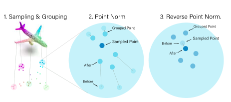
Figure 1: Overview of DualNorm (Point Normalization and Reverse Point Normalization) in our PointNorm framework. After sampling and grouping, we first normalize the grouped points to the sampled points and then normalize the sampled points to the grouped point. In this way, we address the irregularity of the point cloud and facilitate the learning for subsquent layers.

With the success of PointNet++, a handful of works have attempted to exploit the local geometry of point cloud by incorporating convolution [8, 9], graph [10, 11], transformers [12, 13] or geometric methods [14, 15] in the non-linear mapping layers. Unlike the local geometry, the global point features bring long-range semantics, which benefit part segmentation and semantic segmentation [16, 17, 18]. The global geometry exploration of point cloud often involves adaptive sampling [16], mesh [19], curve [17], or surfaces [15].

Despite their improvements in classification and segmentation accuracy, both approaches follow PointNet++’s sampling-grouping operations, which fail to represent the 3D geometry of the irregular point cloud. Without addressing the irregularity issue, these approaches engage in a competition for complex feature extractors and optimization procedures, resulting in extended inference latency. This is unacceptable for large-scale point cloud analysis [20] and mobile point cloud analysis [3], which both emphasize computational efficiency.

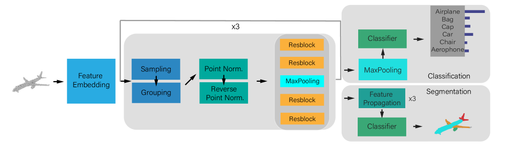
Figure 2: PointNorm for shape classification and part segmentation. Given an input point cloud, PointNorm first embeds the point features and then utilizes sampling-grouping and DualNorm (Point Normalization and Reverse Point Normalization) to normalize sampled and grouped points. The Residual Blocks exploits the hierarchical features to assist the classification and the segmentation head to model the correct category.

In this paper, we seek to eliminate complicated local and/or global feature extractors and develop a simple, intuitive network for point cloud analysis. Inspired by how normalization serves as a pre-processing step to address irregular data in 2D image processing [21, 22], we propose to add normalization after sampling-grouping, but before the non-linear mapping layers. In this way, we can enjoy the efficiency of the sampling-grouping operation while preventing irregular data from passing into the subsequent non-linear mapping layers. Since sampled and grouped points are both crucial for point cloud feature learning, it is hard to decide which one to normalize. Instead of discarding any one of them, we attempt to utilize both points using a novel module called DualNorm. As shown in Fig. 1, the DualNorm module first normalizes the grouped points to the sampled points and then normalizes the sampled points to the grouped points. Using local mean and global standard deviation in the normalization allows the proposed method to leverage local and global features while enjoying a faithful inference speed. The contributions of this paper can be summarized as below:

• We propose a new framework named PointNorm. With local mean and global standard deviation, PointNorm eliminates the need for sophisticated local and global feature extractors, thereby significantly enhancing the computational efficiency.

• We introduce a novel, plug-and-play style module called DualNorm. By normalizing sampled points and grouped points to each other, the DualNorm module uses an adaptive push-and-pull strategy to optimize the point cloud density, thereby addressing the point cloud irregularity.

• We provide analysis to show that DualNorm can remarkably improve the loss stability and gradient stability with a trivial increase in computational complexity.

• We demonstrate that PointNorm achieves compelling performances on point cloud classification and segmentation.

The rest of the paper is organized as follows. Section II provides a comprehensive review of related works. Section III presents the key components of the proposed methods. Section IV outlines the experimental details and provides qualitative and quantitative comparisons. Section V summarizes the findings and discusses the future works.

II Related Work

II-A Point Cloud Analysis

Due to the irregularity of the point cloud data structure, prior works attempt to transform the raw point cloud into intermediate voxels [23, 24], or multi-view images [25, 26], thereby converting the 3D challenge to a well-investigated 2D task. However, these transformations are accompanied by heavy computation and loss of shape details [27, 18]. PointNet [5] is the pioneering method that operates directly upon the raw point cloud. Based upon PointNet, PointNet++ [4] add a sampling-grouping operation before the MLP layers to extract the local geometry. Like PointNet++, and the follow-up works [28, 29, 8, 14], our PointNorm utilizes the sampling-grouping operation with a MLP-based architecture. Unlike previous works, PointNorm leverages normalization between the sampling-grouping layers and the MLP layers to address the irregular point cloud.

II-B Point Cloud Geometry Exploration

Inspired by the success of PointNet++, recent research has greatly explored the point cloud local geometry , using convolutions [8, 9], graphs [10, 11], transformers [12, 11]. The most prominent convolution-based method is PointConv [8], which utilizes MLPs and density functions to obtain the weight function for a given point. Unlike convolution-based methods, graph-based methods (e.g., EdgeConv [10]) treat each point as a graph node and utilize graph edges to capture the local geometry between a specific point and its neighbors, whereas the transformer-based methods like Point Transformer [13] utilize self-attention to extract the local neighborhoods around each point.

The attempt to incorporate global geometry in point cloud analysis is predominantly inspired by the success of non-local network [30] in 2D image processing. The main challenge of point cloud global geometry extraction is how to effectively aggregate the local and the global features [17, 31]. To this end, PointASNL [16] presents a local-nonlocal module with adaptive sampling to capture the local and global dependencies of the sampled point. MeshWalker [19] explores local and global geometry through random walks along the mesh surfaces. CurveNet [17] develops a curve-based guided walk strategy to group and aggregate local-nonlocal point features.

The local and global approaches mentioned above require advanced searching and optimization to collect and combine features, causing poor inference latency. In comparison, the proposed PointNorm enjoys excellent computational efficiency because it only needs normalization operations using the mean of the local points and the standard deviation of the global points (i.e., all points).

III Proposed Methods

In this section, we first introduce DualNorm and then employ standard deviation analysis and optimization landscape analysis to show the superiority of DualNorm. After that, we illustrate the model architecture for PointNorm. Finally, we introduce a lightweight version named PointNorm-Tiny.

III-A DualNorm

III-A1 Preliminaries

PointNet++ [4] performs both sampling and grouping operations on the irregular point cloud. Consequently, the sampled and grouped points are both irregular. Our DualNorm modules consist of Point Normalization (PN) and Reverse Point Normalization (RPN). Specifically, PN aims to address the irregularity of the grouped points, whereas RPN aims to address the irregularity of the sampled points.

III-A2 Notations

Suppose $x_{s}$ represents the sampled points; $x_{g}$ represents the grouped points; $k$ is the number of neighbors in the KNN algorithm [7]; $n$ is the number of points in a point cloud; $d$ is the dimension (i.e., the channel number at a specific layer); $\alpha_{1}$ and $\alpha_{2}$ are learnable parameters initialized with a value of 1; $\beta_{1}$ and $\beta_{2}$ are learnable parameters initialized with a value of 0; $\varepsilon$ is set as $10^{-5}$ to promote numerical stability (e.g., avoid division by zero).

III-A3 Point Normalization

PN normalizes $x_{g}$ to $x_{s}$. The mean $\mu_{s}$ and the standard deviation $\sigma_{1}$ for PN are:

$$\mu_{1}=\begin{cases}x_{s}&$local$\\ \frac{1}{nd}\sum_{b=1}^{n}\sum_{c=1}^{d}x_{s}&$global$\end{cases}$$ (1)

$$\sigma_{1}=\begin{cases}\sqrt{\frac{1}{k}\sum_{a=1}^{k}\left[x_{g_{a}}-\mu_{1}\right]^{2}}&$local$\\ \sqrt{\frac{1}{knd}\sum_{a=1}^{k}\sum_{b=1}^{n}\sum_{c=1}^{d}\left[x_{g_{a,b,c}}-\mu_{1}\right]^{2}}&$global$\end{cases}$$ (2)

The scale-and-shift strategy in batch normalization [32] is employed to promote non-linearity and to make the PN layers trainable in the backpropagation process. The scale-and-shift normalization for PN is

$$x_{g}\leftarrow\alpha_{1}*\frac{x_{g}-\mu_{1}}{\sigma_{1}+\varepsilon}+\beta_{1}$$ (3)

III-A4 Reverse Point Normalization

RPN normalizes $x_{s}$ to $x_{g}$. The mean $\mu_{g}$ and the standard deviation $\sigma_{2}$ for RPN are:

$$\mu_{2}=\begin{cases}\frac{1}{k}\sum_{a=1}^{k}x_{g}&$local$\\ \frac{1}{knd}\sum_{a=1}^{k}\sum_{b=1}^{n}\sum_{c=1}^{d}x_{g}&$global$\end{cases}$$ (4)

$$\sigma_{2}=\begin{cases}\sqrt{\left|x_{s}-\mu_{2}\right|+\varepsilon}&$local$\\ \sqrt{\frac{1}{knd}\sum_{a=1}^{k}\sum_{b=1}^{n}\sum_{c=1}^{d}\left[x_{s_{a,b,c}}-\mu_{2}\right]^{2}}&$global$\end{cases}$$ (5)

The scale-and-shift normalization for RPN is

$$x_{s}\leftarrow\alpha_{2}*\frac{x_{s}-\mu_{2}}{\sigma_{2}+\varepsilon}+\beta_{2}$$ (6)

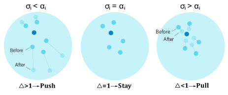
Figure 3: PointNorm’s ‘push-and-pull’ strategy for optimizing the point cloud density. When $\Delta>1$ (left column), PointNorm pushes points apart, which increases the standard deviation and reduces the point cloud density; when $\Delta<1$ (right column), PointNorm pulls points together, which reduces the standard deviation and increase the point cloud density; when $\Delta=1$ (middle column), no action is performed, and both the standard deviation and the point cloud density stay the same.

.

III-A5 Standard Deviation Analysis

We analyze the standard deviation change of point cloud to understand how DualNorm address the irregularity of point cloud. Suppose that the points before and after DualNorm is $x$ and $\hat{x}$, and the standard deviation for $x$ and $\hat{x}$ is $\sigma_{x}$ and $\sigma_{\hat{x}}$. According to the scale-and-shift normalization, we have:

$$\hat{x}=\alpha_{i}*\frac{x-\mu_{i}}{\sigma_{i}+\varepsilon}+\beta_{i}$$ (7)

If we ignore the tiny $\varepsilon$, we can express $\sigma_{\hat{x}}$ as:

$$\sigma_{\hat{x}}=\frac{\alpha_{i}}{\sigma_{i}}*\sigma_{x}$$ (8)

Suppose that the standard deviation change ratio is defined as $\Delta=\frac{\sigma_{\hat{x}}}{\sigma_{x}}$. Equ. 8 can therefore be written as:

$$\Delta=\frac{\alpha_{i}}{\sigma_{i}}$$ (9)

Since $\alpha_{i}$ is a learnable parameter, we are able to adopt customized normalization strategies for three scenarios (See Fig. 3) to address the irregularity of the point cloud.

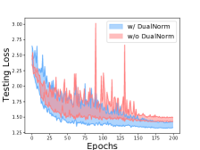
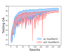
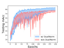
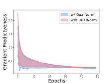
Figure 4: Optimization Landscape Analysis with Testing Loss$\downarrow$, OA$\uparrow$, mAcc$\uparrow$, and Gradient Predictiveness$\downarrow$. Zoom in for a better view.

III-A6 Optimization Landscape Analysis

We perform an optimization landscape analysis [33] on ScanObjectNN [34] to examine the effectiveness of DualNorm. Two PointNorm variants, one with DualNorm, and the other without DualNorm, are investigated with different initial learning rates (0.005, 0.01, 0.002). For each variant, the learning rate configuration leading to the lowest/highest score of a metric is plotted as the lower/upper bound for the shaded region in Fig. 4.

For evaluation metrics, we choose testing loss, OA and mAcc to examine the loss stability (Lipschitzness) and gradient predictiveness (the L2 gradient change) to examine the gradient stability. Fig. 4 shows that PointNorm with DualNorm has less fluctuation and better scores for loss, OA, and mAcc, which means DualNorm help reduce the Lipschitz constant and improve the loss stability during training. Besides, PointNorm with DualNorm has lower gradient predictiveness, especially during the early-stage training. This result indicates DualNorm help reduce the L2 gradient change and ensures better gradient stability during training.

III-B PointNorm

We show the workflow of PointNorm in Fig. 2. PointNorm consists of five steps: feature embedding, sampling-grouping, DualNorm (PN+RPN), non-linear mapping, and classification/segmentation. The feature embedding step aims to raise the channel number so that the network contains more learnable parameters. Inspired by PointNet++ [4], we repeat the sampling-grouping, the DualNorm, and the non-linear mapping step three times to extract the hierarchical features with different receptive fields. The FPS [6] is used for point sampling, whereas KNN with k = 24 [7] is used for point grouping. Following sampling-grouping, we leverage DualNorm to normalize the sampled and the grouped points. Following DualNorm, the sampled and the grouped points are concatenated before entering the subsequent non-linear mapping step. The non-linear mapping step consists of four Residual Blocks and one max pooling layer in the middle for channel number reduction. Finally, inspired by previous works [5, 4, 24, 10], we use max pooling to preserve the salient features for classification, and progressive feature propagation to upsample the point features for segmentation.

III-C PointNorm-Tiny

PointNorm has excellent inference latency and classification accuracy, but many amount of parameters (12.63M). This motivates us to design a lightweight version suitable for mobile deployment. The lightweight version should have few parameters, a high inference latency, and a good classification accuracy. To create PointNorm-Tiny, we make three adjustments. First, we reduce the bottleneck ratio from 1.00 to 0.25. Second, we lower the feature embedding dimension from 64 to 32. Third, we reduce ResBlock by 50%. PointNorm-Tiny has only 0.68M parameters, infers faster than PointNet++, and delivers delivers faithful classification accuracy in the experiments.

IV Experiments

In this section, we first describe the implementation details of PointNorm and then compare PointNorm with state-of-the-art methods on shape classification and part segmentation benchmarks. Finally, we conduct ablation studies to demonstrate the effectiveness of the proposed modules and the reason for the current hyperparameter selection.

IV-A Implementation Details

PointNorm is trained on a single GPU for 200 epochs, using AdamW [35] as the optimizer and cosine annealing [36] as the scheduler. The initial learning rate is 0.01; the minimum learning rate is 0.0001; the batch size is 32; the embedding dimension is 64; it takes approximately 9 hours to converge. We utilize both PN and RPN, adopt local mean and global standard deviation, and choose ResBlock with a bottleneck ratio of 1.0. Inspired by previous works [10, 14], we use cross-entropy with label smoothing [37] as the loss function. Finally, we adopt random rotation and translation [4, 10, 38, 14] as the data augmentation techniques.

TABLE I: Ablation Study Result for PointNorm. FLOPs refer to the floating-point operations for computing a single point cloud. Train/Test Time refers to the seconds per epoch on the training/testing dataset. The best accuracy is in Bold.

		OA (%)	mAcc (%)	FLOPs	#Params	Train Time	Test Time
Layer Number	24	86.5	85.2	8.71G	7.30M	99	9
	40	86.8	85.6	14.59G	12.63M	145	13
	56	86.7	85.0	20.48G	17.95M	190	16
Bottleneck Ratio	0.25	85.9	84.5	5.79G	4.65M	99	9
	0.50	86.6	85.4	8.72G	7.31M	111	10
	1.00	86.8	85.6	14.59G	12.63M	145	13
	2.00	86.6	85.1	26.34G	23.27M	205	17
Local/ Global	LMGS	86.8	85.6	14.59G	12.63M	145	13
	LMLS	81.2	78.3	14.59G	12.63M	145	13
	GMLS	25.1	16.8	14.59G	12.63M	143	13
	GMGS	78.4	75.5	14.59G	12.63M	143	13
Norm.	w/o PN	80.7	77.8	14.59G	12.63M	136	12
	w/o RPN	85.6	84.1	14.59G	12.63M	141	12
	w/ both	86.8	85.6	14.59G	12.63M	145	13

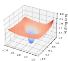
(a) LMGS (w/ Both)

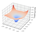
(b) LMGS (w/o PN)

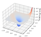
(c) LMGS (w/o RPN)

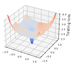
(d) LMLS (w/ Both)

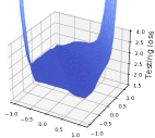
(e) GMLS (w/ Both)

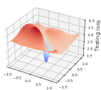
(f) GMGS (w/ Both)

Figure 5: Loss landscape [39] along two random directions for different PointNorm variants. Zoom in to view the details.

TABLE II: Shape Classification Result on ModelNet40 and ScanObjectNN. All methods except PointASNL are tested without the voting strategy. We use overall accuracy (OA) and mean accuracy (mAcc), number of parameters (#Params), train speed and test speed by samples per second computed on a single GPU as the evaluation metrics. We use bold to indicate the best score, and blue for the second-best score. ‘-’ indicate a result is unavailable.

			ModelNet40 [40]		ScanObjectNN [34]
Method	Publication	Input	OA (%)	mAcc (%)	OA (%)	mAcc (%)	#Params	Train Speed	Test Speed
PointNet [5]	CVPR 2017	1k	89.2	86.0	68.2	63.4	3.47M	-	-
PointNet++ [4]	NeurIPS 2017	1k	90.7	88.4	77.9	75.4	1.48M	223.8	308.5
PointCNN [28]	NeurIPS 2018	1k	92.5	88.1	78.5	75.1	-	-	-
DGCNN [10]	TOG 2019	1k	92.9	90.2	78.1	73.6	1.82M	-	-
RS-CNN [29]	CVPR 2019	1k	92.9	-	-	-	2.38M	-	-
PointConv [8]	CVPR 2019	1k	92.5	-	-	-	18.6M	17.9	10.2
KPConv [38]	ICCV 2019	7k	92.9	-	-	-	14.3M	31.0	80.0
PointASNL [16]	CVPR 2020	1k	93.2	-	-	-	10.1M	-	-
Grid-GCN [41]	CVPR 2020	1k	93.1	91.3	-	-	-	-	-
DRNet [42]	WACV 2021	1k	93.1	-	80.3	78.0	-	-	-
PAConv [9]	CVPR 2021	1k	93.6	-	-	-	2.44M	-	-
CurveNet [17]	ICCV 2021	1k	93.8	-	-	-	2.04M	20.8	15.0
GDANet [43]	AAAI 2021	1k	93.4	-	-	-	0.93M	26.3	14.0
PRANet [44]	TIP 2021	1k	93.2	90.6	81.0	77.9	-	-	-
PointMLP [14]	ICLR 2022	1k	94.1	91.3	85.4	83.9	12.60M	47.1	112.0
RepSurf-U [15]	CVPR 2022	1k	-	-	84.6	81.9	1.48M	-	-
PointNorm		1k	94.1	91.3	86.8	85.6	12.63M	58.2	140.0
PointNorm-Tiny		1k	93.5	90.6	85.3	83.6	0.68M	196.4	420.0

TABLE III: Part Segmentation Result on ShapeNetPart. All scores are reported in %. The best score for Instance mIoU and Class mIoU are in bold. Zoom in to view better.

Method	Inst. mIoU	Cls. mIoU	air- plane	bag	cap	car	chair	aero- phone	guitar	knife	lamp	laptop	motor- bike	mug	pistol	rocket	skate- board	table
PointNet [5]	83.7	80.4	83.4	78.7	82.5	74.9	89.6	73.0	91.5	85.9	80.8	95.3	65.2	93.0	81.2	57.9	72.8	80.6
PointNet++ [4]	85.1	81.9	82.4	79.0	87.7	77.3	90.8	71.8	91.0	85.9	83.7	95.3	71.6	94.1	81.3	58.7	76.4	82.6
PCNN [45]	85.1	81.8	82.4	80.1	85.5	79.5	90.8	73.2	91.3	86.0	85.0	95.7	73.2	94.8	83.3	51.0	75.0	81.8
DGCNN [10]	85.2	82.3	84.0	83.4	86.7	77.8	90.6	74.7	91.2	87.5	82.8	95.7	66.3	94.9	81.1	63.5	74.5	82.6
PointCNN [28]	86.1	84.6	84.1	86.5	86.0	80.8	90.6	79.7	92.3	88.4	85.3	96.1	77.2	95.2	84.2	64.2	80.0	83.0
RS-CNN [29]	86.2	84.0	83.5	84.8	88.8	79.6	91.2	81.1	91.6	88.4	86.0	96.0	73.7	94.1	83.4	60.5	77.7	83.6
SyncSpecCNN [46]	84.7	82.0	81.6	81.7	81.9	75.2	90.2	74.9	93.0	86.1	84.7	95.6	66.7	92.7	81.6	60.6	82.9	82.1
SPLATNet [47]	85.4	83.7	83.2	84.3	89.1	80.3	90.7	75.5	92.1	87.1	83.9	96.3	75.6	95.8	83.8	64.0	75.5	81.8
SpiderCNN [48]	85.3	82.4	83.5	81.0	87.2	77.5	90.7	76.8	91.1	87.3	83.3	95.8	70.2	93.5	82.7	59.7	75.8	82.8
PAConv [9]	86.1	84.6	84.3	85.0	90.4	79.7	90.6	80.8	92.0	88.7	82.2	95.9	73.9	94.7	84.7	65.9	81.4	84.0
PointMLP [14]	86.1	84.6	83.5	83.4	87.5	80.5	90.3	78.2	92.2	88.1	82.6	96.2	77.5	95.8	85.4	64.6	83.3	84.3
PointNorm	86.2	84.7	82.7	84.9	88.9	79.8	90.2	81.9	91.6	87.4	82.9	95.8	78.4	95.5	84.5	65.6	81.4	83.8
PointNorm-Tiny	85.6	84.5	82.9	88.0	89.7	79.3	90.1	79.9	91.6	87.7	82.4	95.8	76.3	95.0	83.5	64.6	81.9	83.5

IV-B Ablation Studies

We conduct extensive ablation studies on the ScanObjectNN dataset to demonstrate the effectiveness of the proposed components in PointNorm, and the reason for specific module designs and hyperparameters selections. Specifically, we employ a score table (Table I) and loss landscape visualizations (Fig. 5) to investigate four aspects, including Layer Number, Bottleneck Ratio, Local/Global, and Normalization.

IV-B1 Layer Number

We define the Layer Number as the number of learnable layers in a network except for batch normalization and activation functions. Table I shows that the 40-layer variant gives the best OA and mAcc. That being said, all Layer Number variants of PointNorm (24-layer, 40-layer, 56-layer) have a close OA and mAcc. That demonstrates the robustness of PointNorm to Layer Number in the network.

IV-B2 Bottleneck Ratio

The Bottleneck Ratio of Residual Block [49] offers a convenient trade-off between model size and performance. We consider four bottleneck ratios (0.25, 0.50, 1.00, 2.00) to analyze PointNorm’s performance at different sizes. Table I shows that a Bottleneck ratio of 1.00 is the best choice because it gives the best OA and mAcc.

IV-B3 Local/Global

As mentioned in Subsection III-A, we can choose either Local or Global for calculating the mean and the standard deviation. Therefore, there exist four combinations, including Local Mean Global Standard Deviation (LMGS), Local Mean Local Standard Deviation (LMLS), Global Mean Local Standard Deviation (GMLS), and Global Mean Global Standard Deviation (GMGS). Table I gives us the quick answer: LMGS is the optimal choice.

We visualize the loss landscape in Fig. 5 to better understand the underlying mechanism of DualNorm. We notice that both LMLS and GMGS have sharp minimas and rough surfaces with many hills, which is hard to train. GMLS can hardly be optimized because it has no apparent minima. In comparison, LMGS has a flat minima and a smooth landscape, which remarkably facilities the optimization process [50, 39]. Based on the analysis above, we confirm that LMGS is the best.

IV-B4 Normalization

We investigate the building blocks of DualNorm (PN, RPN) by considering three variants: PointNorm (w/o PN, w/o RPN, w/ both PN and RPN).

Table I shows that PointNorm w/ Both PN and RPN has the best OA and mAcc. Fig. 5 shows that PointNorm w/ both PN and RPN has a flat minima and a smooth surface. While PointNorm w/o PN and PointNorm w/o RPN also have flat minima, they have significant uphills at the border, which may lead to loss explorations. Hence, we conclude that both PN and RPN are essential building blocks of DualNorm.

IV-C Shape Classification

We evaluate PointNorm on shape classification tasks using two benchmark datasets. The first benchmark is ModelNet40 [40], a synthetic dataset with 40 classes, 9,843 training samples, and 581 testing samples. The second benchmark is ScanobjectNN [34], a real-world dataset with 15 classes, 2,321 training samples, and 581 testing samples.

We show the experiment results for shape classification in Table II . For both ModelNet40 and ScanObjectNN, PointNorm has the best OA and mAcc. Notably, on ScanObjectNN, PointNorm surpasses the previous state-of-the-art PointMLP by 1.4% in OA and 1.7% in mAcc. The lightweight version PointNorm-Tiny has the smallest #Params and the best testing speed yet still delivers strong results, surpassing recent state-of-the-arts like PRANet [44] and DRNet [42].

TABLE IV: Semantic Segmentation Result on S3DIS Dataset. mIOU, mAcc and OA are reported in %. The best score is in Bold. ‘-’ indicate a result is unavailable.

Method	S3DIS 6-Fold			S3DIS Area-5			#Params	FLOPs
	mIoU	mAcc	OA	mIoU	mAcc	OA
PointNet [5]	47.6	66.2	78.5	43.2	52.6	77.8	1.7M	4.1G
PointWeb [51]	66.7	76.2	87.3	60.2	66.6	87.0	-	-
KPConv [38]	70.6	79.1	-	67.1	72.8	-	14.9M	-
PointASNL [16]	68.7	79.0	88.8	62.6	68.5	87.7	22.4M	19.1G
RPNet [52]	70.8	-	-	-	-	-	2.4M	5.1G
DSPoint [53]	63.3	70.9	-	-	-	-	-	-
PointNet++ [4]	54.5	67.1	81.0	52.6	63.1	82.3	0.969M	1.00G
PointNet++ (w/ DualNorm)	62.7	73.8	85.7	57.6	68.2	88.4	1.006M	1.05G
(w/ DualNorm)	$\uparrow$8.2	$\uparrow$6.7	$\uparrow$4.7	$\uparrow$5.0	$\uparrow$5.1	$\uparrow$6.1	$\uparrow$0.037M	$\uparrow$0.05G

IV-D Part Segmentation

We evaluate our PointNorm on the part segmentation task, using ShapeNetPart [54] as the benchmark dataset. The ShapeNetPart dataset contains 16,881 shapes, 16 classes, and 50 parts labels. The experiment results for part segmentation in Table III show that PointNorm achieves the best score for both instance mIoU (86.2%) and class mIoU (84.7%). PointNorm-Tiny, albeit being lightweight, delivers compelling instance mIoU (85.6%) and class mIoU (84.5%), close to the recent state-of-the-arts PAConv [9] and PointMLP [14]. We also visualize the part segmentation results in Fig. 6. It can be seen that both PointNorm and PointNorm-Tiny’s predictions are incredibly close to the ground truth.

IV-E Semantic Segmentation

We evaluate PointNorm on the semantic segmentation task, using S3DIS [55] as the benchmark dataset. The S3DIS dataset contains 271 scenes from 6 indoor areas and has 13 semantic labels. In Table IV, we compare PointNorm with other methods on S3DIS 6-Fold and S3DIS Area-5. With a 0.037M increase in #Params, and a 0.05G increase in FLOPs, DualNorm boosts the mIoU, mAcc, and OA for PointNet++ on both S3DIS 6-Fold and Area-5. It is worth mentioning that PointNet++ (w/ DualNorm) has the best OA for S3DIS Area-5, surpassing the recent state-of-the-art PointASML, which has far more #Params and FLOPs. We also visualize the semantic segmentation results in Fig. 7. We can see that PointNet++ (w/o DualNorm) is much closer to the ground truth.

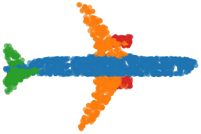
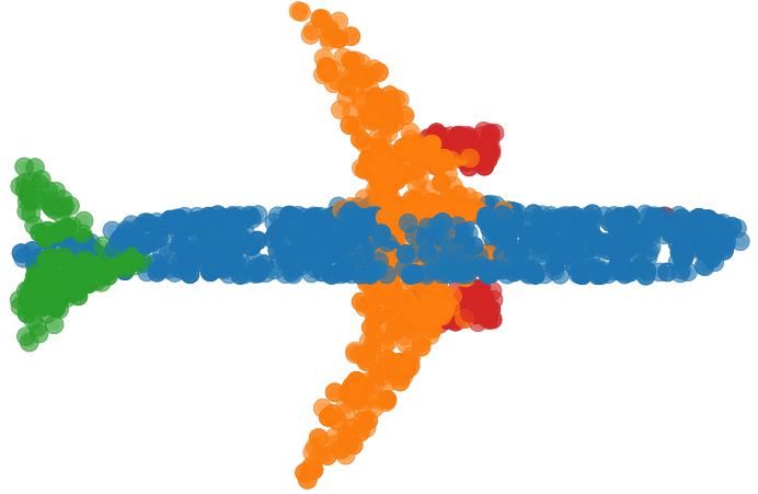
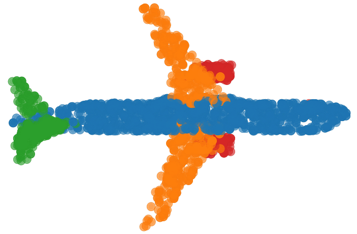
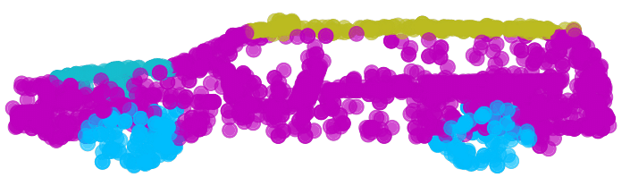
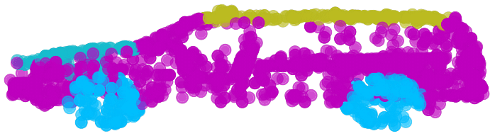
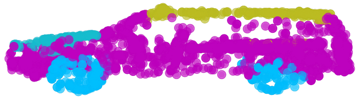
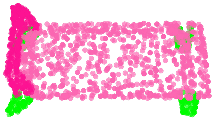
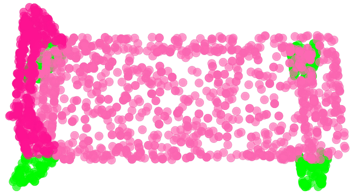
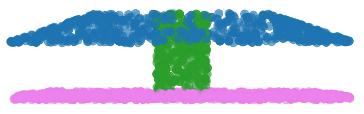
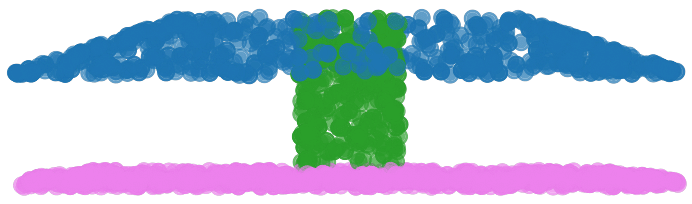
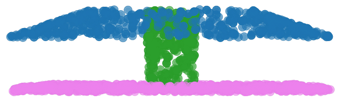
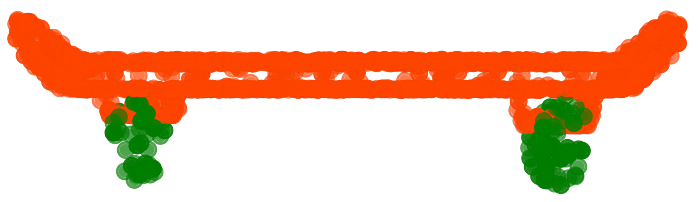
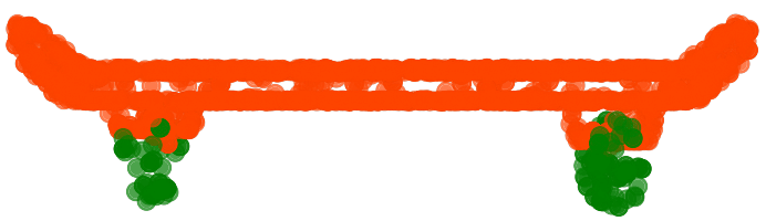
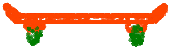
Figure 6: Part Segmentation Result Visualization. From left to right column: Ground Truth, PointNorm, PointNorm-Tiny. From top to bottom row: airplane, car, chair, lamp, skateboard.

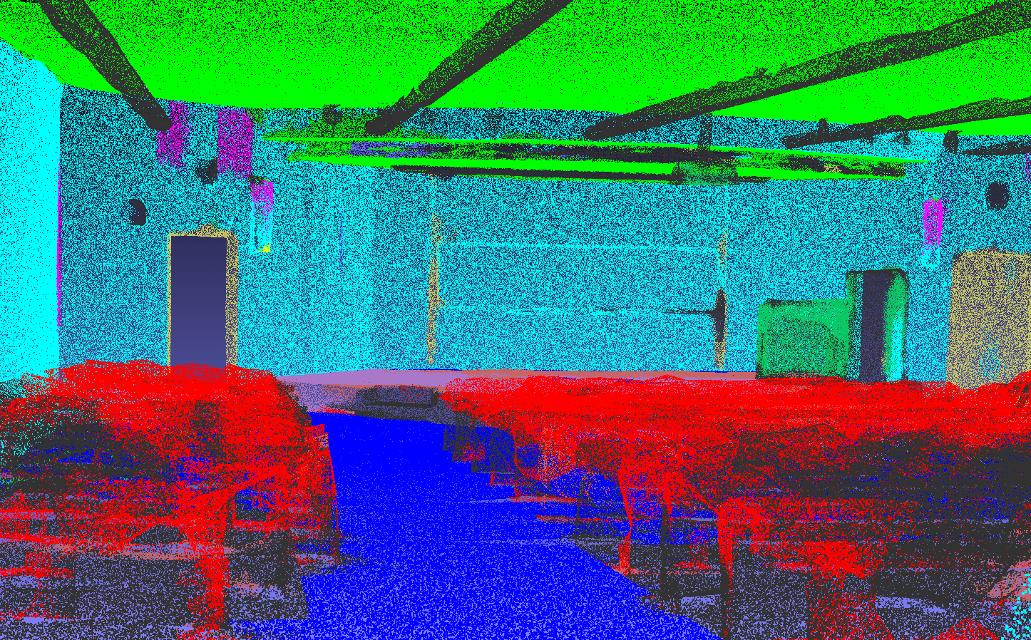
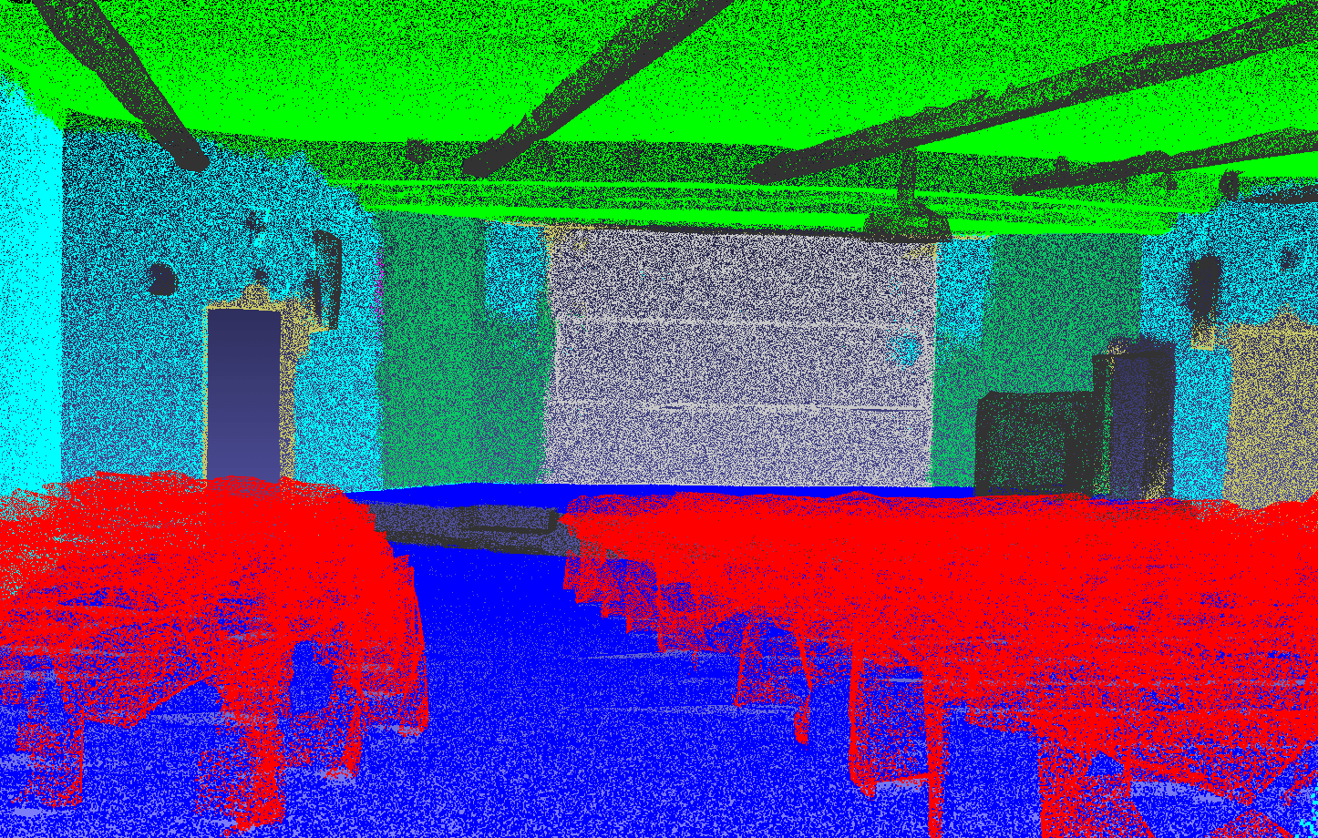
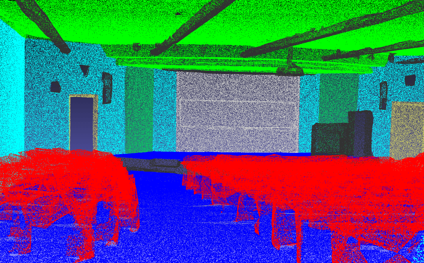
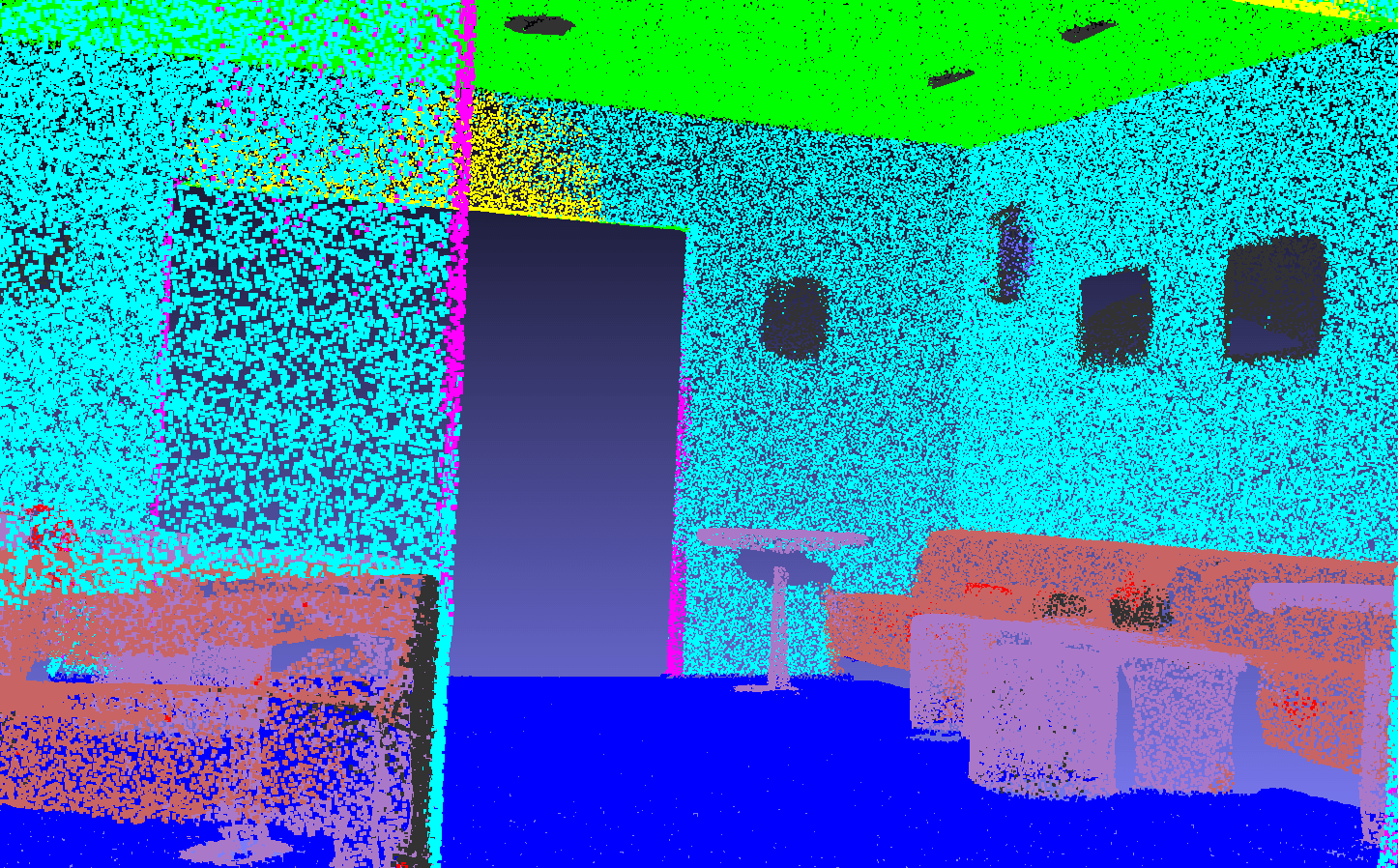
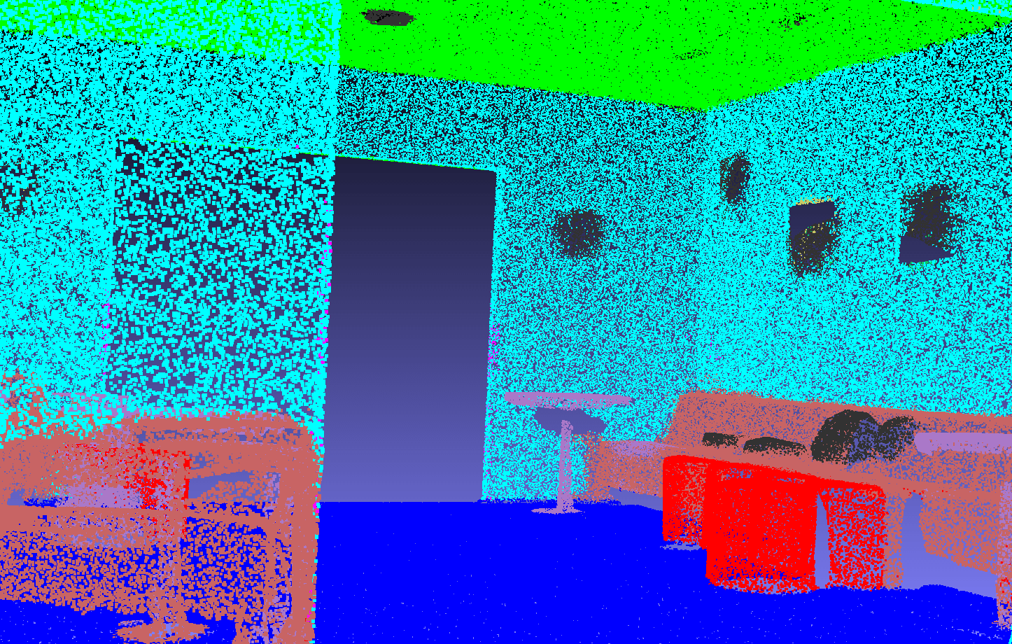
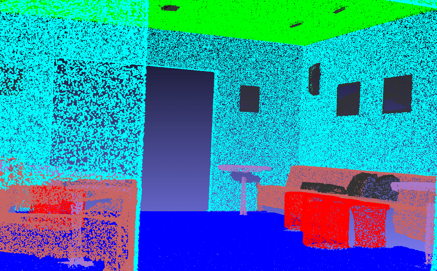
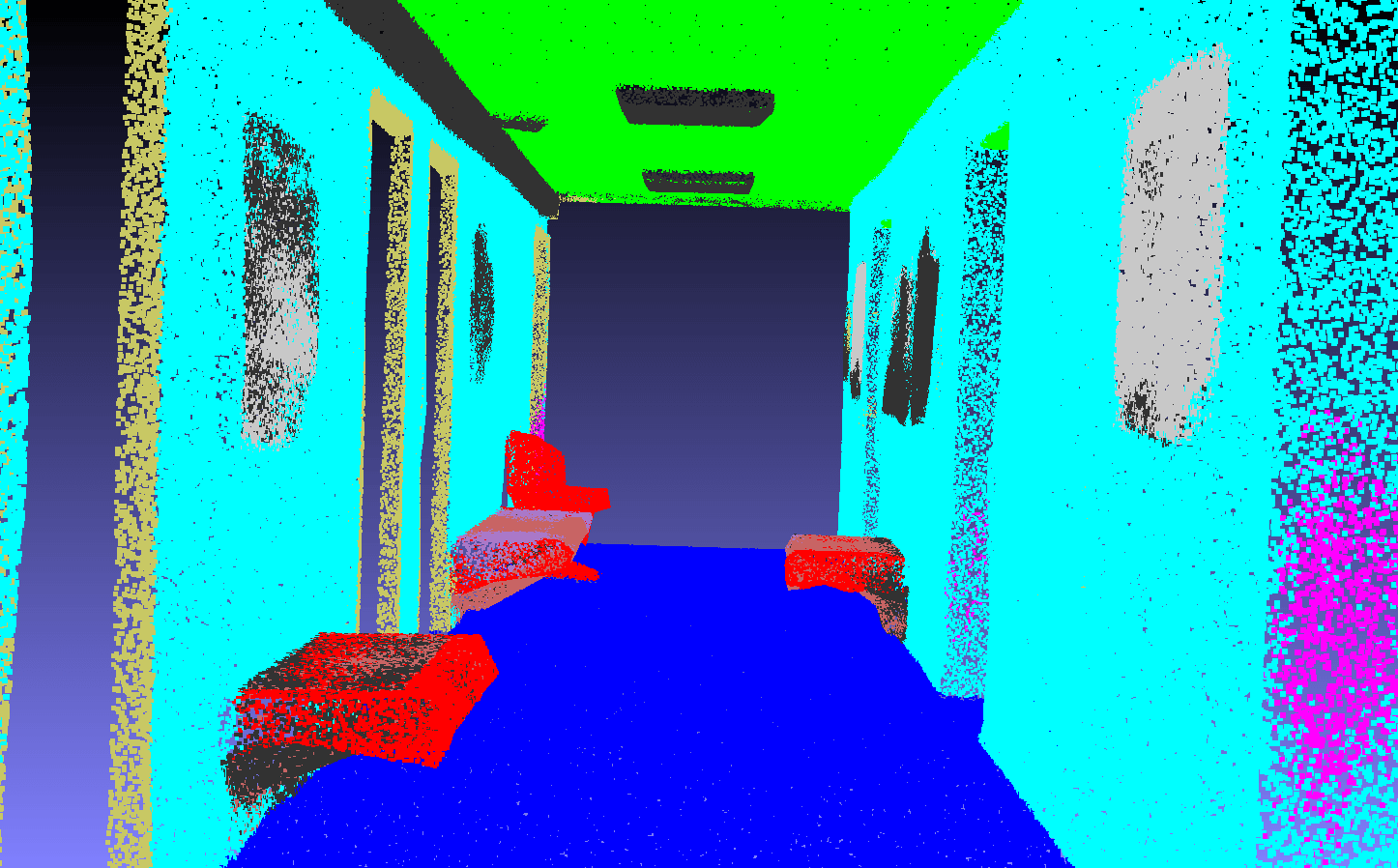
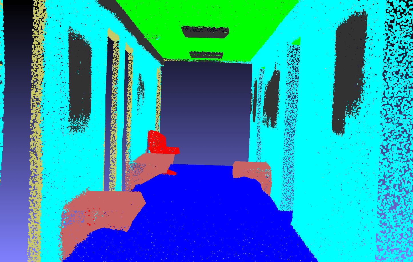
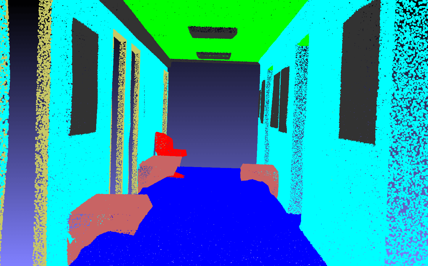
Figure 7: Semantic Segmentation Result Visualization. From left to right column: PointNet++, PointNet++ (w/ DualNorm), Ground Truth. From top to bottom row: auditorium, lounge, hallway. Zoom in to view the details.

V Conclusion

In this paper, we propose PointNorm, an point cloud analysis framework that eliminates the need for sophisticated feature extractors. The key ingredient of PointNorm is the DualNorm module, where we address the point cloud irregularity by normalizing the grouped points and the sampled points to each other using local mean and global standard deviation. This straightforward design benefit both the classification accuracy, computational efficiency, loss stability, and gradient stability. Comprehensive experiments and ablation studies demonstrate the effectiveness of the proposed method. In the future, we plan to apply PointNorm to object detection (e.g., SUN RGB-D [56]) and outdoor semantic segmentation (e.g., SemanticKITTI [57]) tasks. It is also interesting to explore semantic information [58], mutual information [59], and adversarial similarity [60] in our framework.

References

- [1] Siheng Chen, Baoan Liu, Chen Feng, Carlos Vallespi-Gonzalez, and Carl Wellington. 3d point cloud processing and learning for autonomous driving: Impacting map creation, localization, and perception. IEEE Signal Processing Magazine, 38(1):68–86, 2020.
- [2] Dejing Ni, Andrew YC Nee, Soh-Khim Ong, Huijun Li, Chengcheng Zhu, and Aiguo Song. Point cloud augmented virtual reality environment with haptic constraints for teleoperation. Transactions of the Institute of Measurement and Control, 40(15):4091–4104, 2018.
- [3] François Pomerleau, Francis Colas, Roland Siegwart, et al. A review of point cloud registration algorithms for mobile robotics. Foundations and Trends® in Robotics, 4(1):1–104, 2015.
- [4] Charles Ruizhongtai Qi, Li Yi, Hao Su, and Leonidas J Guibas. Pointnet++: Deep hierarchical feature learning on point sets in a metric space. Advances in neural information processing systems, 30, 2017.
- [5] Charles R Qi, Hao Su, Kaichun Mo, and Leonidas J Guibas. Pointnet: Deep learning on point sets for 3d classification and segmentation. In Proceedings of the IEEE conference on computer vision and pattern recognition, pages 652–660, 2017.
- [6] Carsten Moenning and Neil A Dodgson. Fast marching farthest point sampling. Technical report, University of Cambridge, Computer Laboratory, 2003.
- [7] Leif E Peterson. K-nearest neighbor. Scholarpedia, 4(2):1883, 2009.
- [8] Wenxuan Wu, Zhongang Qi, and Li Fuxin. Pointconv: Deep convolutional networks on 3d point clouds. In Proceedings of the IEEE/CVF Conference on Computer Vision and Pattern Recognition, pages 9621–9630, 2019.
- [9] Mutian Xu, Runyu Ding, Hengshuang Zhao, and Xiaojuan Qi. Paconv: Position adaptive convolution with dynamic kernel assembling on point clouds. In Proceedings of the IEEE/CVF Conference on Computer Vision and Pattern Recognition, pages 3173–3182, 2021.
- [10] Yue Wang, Yongbin Sun, Ziwei Liu, Sanjay E Sarma, Michael M Bronstein, and Justin M Solomon. Dynamic graph cnn for learning on point clouds. Acm Transactions On Graphics (tog), 38(5):1–12, 2019.
- [11] Zhi-Hao Lin, Sheng-Yu Huang, and Yu-Chiang Frank Wang. Convolution in the cloud: Learning deformable kernels in 3d graph convolution networks for point cloud analysis. In Proceedings of the IEEE/CVF conference on computer vision and pattern recognition, pages 1800–1809, 2020.
- [12] Meng-Hao Guo, Jun-Xiong Cai, Zheng-Ning Liu, Tai-Jiang Mu, Ralph R Martin, and Shi-Min Hu. Pct: Point cloud transformer. Computational Visual Media, 7(2):187–199, 2021.
- [13] Hengshuang Zhao, Li Jiang, Jiaya Jia, Philip HS Torr, and Vladlen Koltun. Point transformer. In Proceedings of the IEEE/CVF International Conference on Computer Vision, pages 16259–16268, 2021.
- [14] Xu Ma, Can Qin, Haoxuan You, Haoxi Ran, and Yun Fu. Rethinking network design and local geometry in point cloud: A simple residual mlp framework. arXiv preprint arXiv:2202.07123, 2022.
- [15] Haoxi Ran, Jun Liu, and Chengjie Wang. Surface representation for point clouds. In Proceedings of the IEEE/CVF Conference on Computer Vision and Pattern Recognition, pages 18942–18952, 2022.
- [16] Xu Yan, Chaoda Zheng, Zhen Li, Sheng Wang, and Shuguang Cui. Pointasnl: Robust point clouds processing using nonlocal neural networks with adaptive sampling. In Proceedings of the IEEE/CVF Conference on Computer Vision and Pattern Recognition, pages 5589–5598, 2020.
- [17] Tiange Xiang, Chaoyi Zhang, Yang Song, Jianhui Yu, and Weidong Cai. Walk in the cloud: Learning curves for point clouds shape analysis. In Proceedings of the IEEE/CVF International Conference on Computer Vision, pages 915–924, 2021.
- [18] Saifullahi Aminu Bello, Shangshu Yu, Cheng Wang, Jibril Muhmmad Adam, and Jonathan Li. Deep learning on 3d point clouds. Remote Sensing, 12(11):1729, 2020.
- [19] Alon Lahav and Ayellet Tal. Meshwalker: Deep mesh understanding by random walks. ACM Transactions on Graphics (TOG), 39(6):1–13, 2020.
- [20] Loic Landrieu and Martin Simonovsky. Large-scale point cloud semantic segmentation with superpoint graphs. In Proceedings of the IEEE conference on computer vision and pattern recognition, pages 4558–4567, 2018.
- [21] S Patro and Kishore Kumar Sahu. Normalization: A preprocessing stage. arXiv preprint arXiv:1503.06462, 2015.
- [22] Dmitry Ulyanov, Andrea Vedaldi, and Victor Lempitsky. Instance normalization: The missing ingredient for fast stylization. arXiv preprint arXiv:1607.08022, 2016.
- [23] Daniel Maturana and Sebastian Scherer. Voxnet: A 3d convolutional neural network for real-time object recognition. In 2015 IEEE/RSJ international conference on intelligent robots and systems (IROS), pages 922–928. IEEE, 2015.
- [24] Yin Zhou and Oncel Tuzel. Voxelnet: End-to-end learning for point cloud based 3d object detection. In Proceedings of the IEEE conference on computer vision and pattern recognition, pages 4490–4499, 2018.
- [25] Haoxuan You, Yifan Feng, Rongrong Ji, and Yue Gao. Pvnet: A joint convolutional network of point cloud and multi-view for 3d shape recognition. In Proceedings of the 26th ACM international conference on Multimedia, pages 1310–1318, 2018.
- [26] Abdullah Hamdi, Silvio Giancola, and Bernard Ghanem. Mvtn: Multi-view transformation network for 3d shape recognition. In Proceedings of the IEEE/CVF International Conference on Computer Vision, pages 1–11, 2021.
- [27] Zetong Yang, Yanan Sun, Shu Liu, Xiaoyong Shen, and Jiaya Jia. Std: Sparse-to-dense 3d object detector for point cloud. In Proceedings of the IEEE/CVF international conference on computer vision, pages 1951–1960, 2019.
- [28] Yangyan Li, Rui Bu, Mingchao Sun, Wei Wu, Xinhan Di, and Baoquan Chen. Pointcnn: Convolution on x-transformed points. Advances in neural information processing systems, 31, 2018.
- [29] Yongcheng Liu, Bin Fan, Shiming Xiang, and Chunhong Pan. Relation-shape convolutional neural network for point cloud analysis. In Proceedings of the IEEE/CVF Conference on Computer Vision and Pattern Recognition, pages 8895–8904, 2019.
- [30] Xiaolong Wang, Ross Girshick, Abhinav Gupta, and Kaiming He. Non-local neural networks. In Proceedings of the IEEE conference on computer vision and pattern recognition, pages 7794–7803, 2018.
- [31] Yulan Guo, Hanyun Wang, Qingyong Hu, Hao Liu, Li Liu, and Mohammed Bennamoun. Deep learning for 3d point clouds: A survey. IEEE transactions on pattern analysis and machine intelligence, 43(12):4338–4364, 2020.
- [32] Sergey Ioffe and Christian Szegedy. Batch normalization: Accelerating deep network training by reducing internal covariate shift. In International conference on machine learning, pages 448–456. PMLR, 2015.
- [33] Shibani Santurkar, Dimitris Tsipras, Andrew Ilyas, and Aleksander Madry. How does batch normalization help optimization? Advances in neural information processing systems, 31, 2018.
- [34] Mikaela Angelina Uy, Quang-Hieu Pham, Binh-Son Hua, Thanh Nguyen, and Sai-Kit Yeung. Revisiting point cloud classification: A new benchmark dataset and classification model on real-world data. In Proceedings of the IEEE/CVF international conference on computer vision, pages 1588–1597, 2019.
- [35] Ilya Loshchilov and Frank Hutter. Decoupled weight decay regularization. arXiv preprint arXiv:1711.05101, 2017.
- [36] Ilya Loshchilov and Frank Hutter. Sgdr: Stochastic gradient descent with warm restarts. arXiv preprint arXiv:1608.03983, 2016.
- [37] Christian Szegedy, Vincent Vanhoucke, Sergey Ioffe, Jon Shlens, and Zbigniew Wojna. Rethinking the inception architecture for computer vision. In Proceedings of the IEEE conference on computer vision and pattern recognition, pages 2818–2826, 2016.
- [38] Hugues Thomas, Charles R Qi, Jean-Emmanuel Deschaud, Beatriz Marcotegui, François Goulette, and Leonidas J Guibas. Kpconv: Flexible and deformable convolution for point clouds. In Proceedings of the IEEE/CVF international conference on computer vision, pages 6411–6420, 2019.
- [39] Hao Li, Zheng Xu, Gavin Taylor, Christoph Studer, and Tom Goldstein. Visualizing the loss landscape of neural nets. Advances in neural information processing systems, 31, 2018.
- [40] Zhirong Wu, Shuran Song, Aditya Khosla, Fisher Yu, Linguang Zhang, Xiaoou Tang, and Jianxiong Xiao. 3d shapenets: A deep representation for volumetric shapes. In Proceedings of the IEEE conference on computer vision and pattern recognition, pages 1912–1920, 2015.
- [41] Qiangeng Xu, Xudong Sun, Cho-Ying Wu, Panqu Wang, and Ulrich Neumann. Grid-gcn for fast and scalable point cloud learning. In Proceedings of the IEEE/CVF Conference on Computer Vision and Pattern Recognition, pages 5661–5670, 2020.
- [42] Shi Qiu, Saeed Anwar, and Nick Barnes. Dense-resolution network for point cloud classification and segmentation. In Proceedings of the IEEE/CVF Winter Conference on Applications of Computer Vision, pages 3813–3822, 2021.
- [43] Mutian Xu, Junhao Zhang, Zhipeng Zhou, Mingye Xu, Xiaojuan Qi, and Yu Qiao. Learning geometry-disentangled representation for complementary understanding of 3d object point cloud. In Proceedings of the AAAI Conference on Artificial Intelligence, volume 35, pages 3056–3064, 2021.
- [44] Silin Cheng, Xiwu Chen, Xinwei He, Zhe Liu, and Xiang Bai. Pra-net: Point relation-aware network for 3d point cloud analysis. IEEE Transactions on Image Processing, 30:4436–4448, 2021.
- [45] Matan Atzmon, Haggai Maron, and Yaron Lipman. Point convolutional neural networks by extension operators. arXiv preprint arXiv:1803.10091, 2018.
- [46] Li Yi, Hao Su, Xingwen Guo, and Leonidas J Guibas. Syncspeccnn: Synchronized spectral cnn for 3d shape segmentation. In Proceedings of the IEEE conference on computer vision and pattern recognition, pages 2282–2290, 2017.
- [47] Hang Su, Varun Jampani, Deqing Sun, Subhransu Maji, Evangelos Kalogerakis, Ming-Hsuan Yang, and Jan Kautz. Splatnet: Sparse lattice networks for point cloud processing. In Proceedings of the IEEE conference on computer vision and pattern recognition, pages 2530–2539, 2018.
- [48] Yifan Xu, Tianqi Fan, Mingye Xu, Long Zeng, and Yu Qiao. Spidercnn: Deep learning on point sets with parameterized convolutional filters. In Proceedings of the European Conference on Computer Vision (ECCV), pages 87–102, 2018.
- [49] Kaiming He, Xiangyu Zhang, Shaoqing Ren, and Jian Sun. Deep residual learning for image recognition. In Proceedings of the IEEE conference on computer vision and pattern recognition, pages 770–778, 2016.
- [50] Nitish Shirish Keskar, Dheevatsa Mudigere, Jorge Nocedal, Mikhail Smelyanskiy, and Ping Tak Peter Tang. On large-batch training for deep learning: Generalization gap and sharp minima. arXiv preprint arXiv:1609.04836, 2016.
- [51] Hengshuang Zhao, Li Jiang, Chi-Wing Fu, and Jiaya Jia. Pointweb: Enhancing local neighborhood features for point cloud processing. In Proceedings of the IEEE/CVF conference on computer vision and pattern recognition, pages 5565–5573, 2019.
- [52] Haoxi Ran, Wei Zhuo, Jun Liu, and Li Lu. Learning inner-group relations on point clouds. In Proceedings of the IEEE/CVF International Conference on Computer Vision, pages 15477–15487, 2021.
- [53] Renrui Zhang, Ziyao Zeng, Ziyu Guo, Xinben Gao, Kexue Fu, and Jianbo Shi. Dspoint: Dual-scale point cloud recognition with high-frequency fusion. arXiv preprint arXiv:2111.10332, 2021.
- [54] Li Yi, Vladimir G Kim, Duygu Ceylan, I-Chao Shen, Mengyan Yan, Hao Su, Cewu Lu, Qixing Huang, Alla Sheffer, and Leonidas Guibas. A scalable active framework for region annotation in 3d shape collections. ACM Transactions on Graphics (ToG), 35(6):1–12, 2016.
- [55] Iro Armeni, Ozan Sener, Amir R Zamir, Helen Jiang, Ioannis Brilakis, Martin Fischer, and Silvio Savarese. 3d semantic parsing of large-scale indoor spaces. In Proceedings of the IEEE conference on computer vision and pattern recognition, pages 1534–1543, 2016.
- [56] Shuran Song, Samuel P Lichtenberg, and Jianxiong Xiao. Sun rgb-d: A rgb-d scene understanding benchmark suite. In Proceedings of the IEEE conference on computer vision and pattern recognition, pages 567–576, 2015.
- [57] Jens Behley, Martin Garbade, Andres Milioto, Jan Quenzel, Sven Behnke, Cyrill Stachniss, and Jurgen Gall. Semantickitti: A dataset for semantic scene understanding of lidar sequences. In Proceedings of the IEEE/CVF International Conference on Computer Vision, pages 9297–9307, 2019.
- [58] Shen Zheng and Gaurav Gupta. Semantic-guided zero-shot learning for low-light image/video enhancement. In Proceedings of the IEEE/CVF Winter Conference on Applications of Computer Vision, pages 581–590, 2022.
- [59] Changjie Lu, Shen Zheng, and Gaurav Gupta. Unsupervised domain adaptation for cardiac segmentation: Towards structure mutual information maximization. In Proceedings of the IEEE/CVF Conference on Computer Vision and Pattern Recognition, pages 2588–2597, 2022.
- [60] Changjie Lu, Shen Zheng, Zirui Wang, Omar Dib, and Gaurav Gupta. As-introvae: Adversarial similarity distance makes robust introvae. arXiv preprint arXiv:2206.13903, 2022.